Numerical study of the Kadomtsev–Petviashvili equation and dispersive shock waves

Abstract

A detailed numerical study of the long time behaviour of dispersive shock waves in solutions to the Kadomtsev-Petviashvili (KP) I equation is presented. It is shown that modulated lump solutions emerge from the dispersive shock waves. For the description of dispersive shock waves, Whitham modulation equations for KP are obtained. It is shown that the modulation equations near the soliton line are hyperbolic for the KPII equation while they are elliptic for the KPI equation leading to a focusing effect and the formation of lumps. Such a behaviour is similar to the appearance of breathers for the focusing nonlinear Schrödinger equation in the semiclassical limit.

Keywords: Kadomtsev-Petviashvili equation, dispersive shock waves, Whitham modulation equations

1 Introduction

We consider the Cauchy problem for the Kadomtsev Petviashvili (KP) equation

$$(u_{t}+uu_{x}+\epsilon^{2}u_{xxx})_{x}+\alpha u_{yy}=0,\quad\alpha=\pm 1,$$ (1)

in the class of rapidly decreasing smooth initial data. Here $\epsilon>0$ is a small parameter and we are interested in the behaviour of the solution $u(x,y,t;\epsilon)$ as $\epsilon\to 0$. In such a limit the solution of the KP equation develops strong oscillations and very high peaks that will be the subject of the present manuscript. The equation (1) was first introduced by Kadomtsev and Petviashvili [22] in order to study the stability of the Korteweg–de Vries (KdV) soliton in a two-dimensional setting, and it is now a prototype for the evolution of weakly nonlinear quasi-unidirectional waves of small amplitude in various physical situations. For $\alpha=-1$ ($\alpha=1)$ the equation (1) is called KPI (KPII) equation and describes quasi-unidirectional long waves in shallow water with weak transversal effects and strong (weak) surface tension. The KPII equation is known to have a defocusing effect, whereas the KPI equation is focusing. It is exactly this latter effect which we will study in this paper. A comparison of the solutions of the two KP equations for the same initial data is shown in Fig. 1 where one can see the focusing effect of KPI.

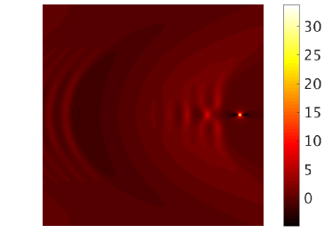
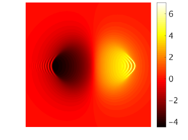
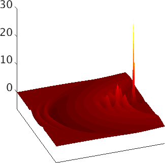
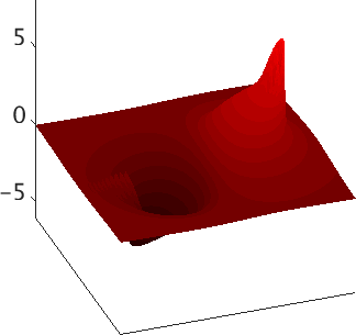
Figure 1: Solution of the KPI equation (left) and of the KPII equation (right) for $\epsilon=0.1$ and the initial data $u(x,y,0)=-6\partial_{x}\mbox{sech}^{2}x$ at time $t=0.8$. Notice how the KPI solution has developed a spike that is about 5 times higher than the highest peak of the KPII solution.

The KP equation is also the prototypical integrable equation [9] in two spatial dimensions and it has been studied via inverse scattering [15] [6]. In the dimensionless KP equation, i.e., equation (1) with $\epsilon=1$, a parameter $\epsilon$ is introduced by considering the long time behavior of solutions with slowly varying initial data of the form $u_{0}(\epsilon x,\epsilon y)$ where $0<\epsilon\ll 1$ is a small parameter and $u_{0}(x,y)$ is some given initial profile. As $\epsilon\to 0$ the initial datum approaches a constant value and in order to see nontrivial effects one has to wait for times of order $t\simeq O(1/\epsilon),$ which consequently requires to rescale the spatial variables onto macroscopically large scales $x\simeq O(1/\epsilon)$, too. This is equivalent to consider the rescaled variables $x\to x^{\prime}=x\epsilon,$ $y\to y^{\prime}=y\epsilon$, $t\to t^{\prime}=t\epsilon$ and put $u^{\epsilon}(x^{\prime},y^{\prime},t^{\prime})=u(x\epsilon,y\epsilon,t\epsilon)$ to obtain the equation (1) where we omit the ^′ for simplicity.

For $\epsilon=0$ the KP equation turns into the so called dispersion-less KP equation (dKP) [30] ,[41]

$$(u_{t}+uu_{x})_{x}+\alpha u_{yy}=0.$$ (2)

Note that in spite of its name, the dKP equation (2) contains dispersion, and only the highest order dispersive term has been dropped relative to (1). Local well-posedness of the Cauchy problem for the dKP equation has been proved in certain Sobolev spaces in [37]. Generically, the solution of the dKP equation develops a singularity in finite time $t_{c}>0$. It is discussed in [18] and [31] that this singularity develops in a point where the gradients become divergent in all directions except one.

As long as the gradients of the dKP solution remain bounded, the solution $u(x,y,t;\epsilon)$ of the KP equation is expected to be approximated in the limit $\epsilon\to 0$ by the solution of the dKP equation. Even if there are many strong results about the Cauchy problem for the KP equation in various functional spaces (see, e.g., [7, 33]), these results are insufficient to rigorously justify the small $\epsilon$ behaviour of solutions to KP even for $0<t<t_{c}$. Near $t=t_{c}$ the solution of the KP equation, preventing the formation of the strong gradients in the dKP solution, starts to develop a region of rapid modulated oscillations. These oscillations are called dispersive shock waves, and they can be approximated at the onset of their formation by a particular solution of the Painlevé I2 equation, up to shifts and rescalings [11].

For later times $t>t_{c}$ these oscillations are expected to be described by the modulated travelling cnoidal wave solution of the KP equation. The travelling cnoidal wave solution is given by

$$u(x,y,t;\epsilon)=\beta_{1}+\beta_{3}-\beta_{2}+2(\beta_{2}-\beta_{3})\mbox{cn}^{2}\left(\dfrac{\sqrt{\beta_{1}-\beta_{3}}}{\sqrt{6}\epsilon}(x+\frac{l}{k}y-\frac{\omega}{k}t)+\phi_{0};m\right)$$ (3)

where $\mbox{cn}(z;m)$ is the Jacobi elliptic function of modulus $m=\dfrac{\beta_{2}-\beta_{3}}{\beta_{1}-\beta_{3}}$ with the constants $\beta_{1}>\beta_{2}>\beta_{3}$, $\phi_{0}$ is an arbitrary constant and $K(m)$ the complete elliptic integral of the first kind. The wave number $k$ and the frequency $\omega$ are given by

$$k=\pi\dfrac{\sqrt{\beta_{1}-\beta_{3}}}{\sqrt{6}K(m)},\quad\omega=\dfrac{k}{3}(\beta_{1}+\beta_{2}+\beta_{3})+\alpha\dfrac{l^{2}}{k}.$$ (4)

The average value $\bar{u}$ over a period and the maximum amplitude $a:=u_{max}-u_{min}$ of the oscillations are

$$\bar{u}=\beta_{2}+\beta_{3}-\beta_{1}+2(\beta_{1}-\beta_{3})\dfrac{E(m)}{K(m)},\quad a=2(\beta_{2}-\beta_{3}),$$ (5)

where $E(m)$ is the complete elliptic integral of the second kind. For constant values of $\beta_{1},\beta_{2},\beta_{3}$ and $l$, the formula (3) gives an exact solution of the KP equation. The modulation of the wave-parameters of the cnoidal wave solution is obtained by letting $\beta_{j}=\beta_{j}(x,y,t)$, $j=1,2,3$ and $l=l(x,y,t)$ and requesting that (3) is an approximate solution of KP up to higher order corrections. Over the last forty years, since the seminal paper of Gurevich and Pitaevsky, [19] there has been a lot of attention to the quantitative study of dispersive shock waves see e.g. the recent volume [4], and refined experiments have been developed [39]. Most of the analysis is restricted to models in one spatial dimension. Two dimensional models have been much less studied, see for example [20],[35],[12]. Regarding the KP equation, the formation of dispersive shock waves has been studied numerically in [27, 24] and both numerically and analytically in [1] for an initial step with parabolic profile, and recently in [5] using the method of multiple scales. Modulation theory in the general setting of Riemann surfaces has been developed in [29]. In this manuscript we derive the modulation equations for KP using the Whitham averaging method over the Lagrangian as in [40]. Our final form of the equations for $\beta_{1}(x,y,t)>\beta_{2}(x,y,t)>\beta_{3}(x,y,t)$ and $q(x,y,t):=l(x,y,t)/k(x,y,t)$, plus two extra dependent variables $p=p(x,y,t)$ and $r=r(x,y,t)$ (see definition (28 and (29)) is

$$\dfrac{\partial}{\partial t}\beta_{i}+(v_{i}+\alpha q^{2})\dfrac{\partial}{\partial x}\beta_{i}+\alpha(2qD\beta_{i}-(v_{i}-2\beta_{i})Dq+Dp)=0,\quad i=1,2,3,$$ (6)

$$\dfrac{\partial}{\partial t}q+\left(\dfrac{1}{3}\sum_{i=1}^{3}\beta_{i}+\alpha q^{2}\right)q_{x}+2\alpha Dq+\dfrac{1}{3}D(\sum_{i=1}^{3}\beta_{i})=0,$$ (7)

$$p_{t}+\left(\dfrac{1}{3}\sum_{i=1}^{3}\beta_{i}+\alpha q^{2}\right)p_{x}+Dr=0,\;\;r_{x}-\dfrac{B_{x}}{6}-\alpha(\bar{u}(q_{y}-qq_{x})+p_{y}+qp_{x}))=0,$$ (8)

with $D=\dfrac{\partial}{\partial y}-q\dfrac{\partial}{\partial x}$, the speeds $v_{i}=v_{i}(\beta_{1},\beta_{2},\beta_{3})$ are

$$v_{i}=\dfrac{1}{3}(\beta_{1}+\beta_{2}+\beta_{3})+\dfrac{2}{3}\dfrac{\prod_{k\neq i}(\beta_{i}-\beta_{k})}{\beta_{i}-\beta_{1}+(\beta_{1}-\beta_{3})\dfrac{E(m)}{K(m)}},\quad i=1,2,3,$$ (9)

with $\bar{u}$ defined in (5) and $B=\sum_{i=1}^{3}\beta_{i}^{2}-2(\beta_{1}\beta_{2}+\beta_{2}\beta_{3}+\beta_{1}\beta_{3})$. The system satisfies two compatibility conditions given by the constraints

$$q_{x}=\dfrac{k_{y}}{k}-q\dfrac{k_{x}}{k},\;\;\;p_{x}=\bar{u}_{y}-(q\bar{u})_{x}.\;\;\;$$ (10)

When $\alpha=0$ the equations (6) and the second equation in (8) coincide with the Whitham modulation equations for KdV with $r=B/6$ being an integral. The equations (6), (7) and (10) are equivalent to the equations obtained in [5], while the equations (8) seem to be new. We set up the Cauchy problem for the Whitham modulation equations and we show that the Whitham system near the solitonic front when $m\simeq 1$ is not hyperbolic.

When the modulus $m\to 1$, the travelling wave solution (3) of KP converges to

$$u(x,y,t;\epsilon)\simeq\beta_{3}+2(\beta_{1}-\beta_{3})\mbox{sech}^{2}\left(\frac{\sqrt{\beta_{1}-\beta_{3}}}{\sqrt{6}\epsilon}(x+\frac{l}{k}y-\frac{\omega}{k})t+\phi_{0}\right).$$ (11)

If we set $\beta_{3}=0$ and $\beta_{1}=6k^{2}$, the above expression is exactly the line soliton of the KP equation and the wave numbers $k$, $l$ and $\omega$ satisfy the dispersion relation $\omega=4k^{3}+\dfrac{\alpha l^{2}}{k}$ (see e.g. [2]). For the KPI equation the line soliton is known to be linearly unstable under perturbations, [42], [36]. Numerical studies as [21], see also the more recent papers [25, 27], and analytical studies [34] indicate that the solitons of the form (11) of sufficient amplitude are unstable against the formation of so called lump solutions.

Lumps are localised solutions decreasing algebraically at infinity that take the form

$$u(x,y,t;\epsilon)=24\dfrac{(-\frac{1}{\epsilon^{2}}(x+ay+(a^{2}-3b^{2})t)^{2}+3\frac{b^{2}}{\epsilon^{2}}(y+2at)^{2}+1/b^{2})}{(\frac{1}{\epsilon^{2}}(x+ay+(a^{2}-3b^{2})t)^{2}+3\frac{b^{2}}{\epsilon^{2}}(y+2at)^{2}+1/b^{2})^{2}},$$ (12)

where $a$ and $b$ are arbitrary constants. The maximum of the lump is located at

$$x=3b^{2}t+a^{2}t,\quad y=-2at,$$

with maximum value $24b^{2}$. When $a=0$ the lump is symmetric with respect to $y$-axis.

We obtain, using the averaging over Lagrangian density, the modulation of the soliton parameters. These equations are elliptic for KPI and therefore they are expected to develop a point of elliptic umbilic catastrophe as for the semiclassical limit of the focusing nonlinear Schrödinger (NLS) equation [11]. In the NLS case a train of Peregrine breathers is generically formed [3] that is in amplitude three times the value of the solution at the point of elliptic umbilic catastrophe. Furthermore the position of the breathers scales in $\epsilon$ with the power $4/5$. The soliton front of the dispersive shock waves for KPI breaks into a lattice of lumps and the distance among the lumps scales with $\epsilon$, see Fig. 2

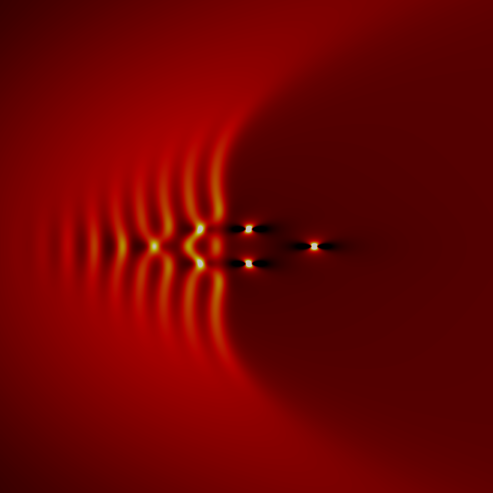
(a) $\epsilon=0.05$, $C_{0}=6$, $t=0.8$

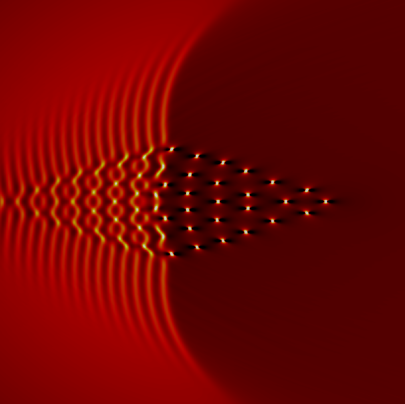
(b) $\epsilon=0.02$, $C_{0}=6$, $t=0.8$

Figure 2: Detail of the lattice arrangement of the lumps on the $(x,y)$ plane for two representative cases for the initial data $u_{0}(x,u)=-C_{0}\partial_{x}\operatorname{sech}^{2}\sqrt{x^{2}+y^{2}}$. The distance between the lumps clearly scales with $\epsilon$.

The amplitude of the first lump that appears is proportional to the initial data and, for the specific initial data considered, it is about ten times the maximal amplitude of the initial data. The amplitude of the lump decreases (numerically) with time, without producing any radiation as in [32]. Finally we study the dependence on $\epsilon$ of the position and the time of formation of the first lump and we find a scaling exponent that is compatible with the value $4/5$ as in the NLS case.

This manuscript is organised as follows. In section 2 we derive the Whitham modulation equations for KP using the averaging over the Lagrangian. We then define the Cauchy problem for the Whitham modulation equations. Next we obtain the modulation equations of the soliton parameters and show that for KPI such equations are elliptic. We then show that the Whitham system is not hyperbolic near the soliton front, since two eigenvalues of the velocity matrix are complex. In section 3 we collect known results on the focusing NLS equation and on how solutions to the NLS equation are related to KPI solutions. In section 4 we briefly present the numerical methods used for the integration of the KP equation. These methods are applied in section 5 to concrete examples for the KPI equation. In particular we study numerically the nature of the lattice of lumps that is formed out of the soliton front in the KPI solution in the small dispersion limit. We add some concluding remarks in section 6.

2 Whitham modulation equations for KP via Lagrangian averaging

In this section we will obtain the Whitham modulation equations for the KP equations following Whitham method [40] of averaged Lagrangian as in [21].

2.1 Lagrangian density for the travelling wave solution of KP

The Lagrangian density of the KP equation is

$$L=\epsilon^{2}f_{t}f_{x}+\dfrac{\epsilon^{3}}{3}f_{x}^{3}-\epsilon^{4}f_{xx}^{2}+\epsilon^{2}\alpha f_{y}^{2}$$ (13)

which leads to the Euler-Lagrange equation

$$f_{tx}+\epsilon f_{x}f_{xx}+\epsilon^{2}f_{xxxx}+\alpha f_{yy}=0.$$

The above equation coincides with the KP equation under the substitution $\epsilon f_{x}=u$. We look for a solution that is a travelling wave, namely a solution of the form

$$f=\psi+\phi(\theta),\quad\theta=\frac{kx+ly-\omega t}{\epsilon},\quad\psi=\frac{c_{1}x+c_{2}y-\gamma t}{\epsilon},$$

where $\phi(\theta)$ is a $2\pi$ periodic function of its argument and the remaining quantities are parameters to be determined. In our notation $x/\epsilon$, $y/\epsilon$ and $t/\epsilon$ will be the fast variables and $x,y$ and $t$ will be the slow variables. We introduce

$$\eta=\epsilon f_{x}=c_{1}+k\phi_{\theta},\quad\epsilon f_{y}=c_{2}+\dfrac{l}{k}(\eta-c_{1}),\quad\epsilon f_{t}=-\gamma-\dfrac{\omega}{k}(\eta-c_{1}).$$

It follows from (1) that the function $\eta(\theta)$ satisfies the equation

$$3k^{2}\eta_{\theta}^{2}=-\eta^{3}+V\eta^{2}+B\eta+A,\$$ (14)

where $B$ and $A$ are integration constants and

$$V=3\left(\dfrac{\omega}{k}-\alpha\dfrac{l^{2}}{k^{2}}\right).$$ (15)

In order to get a periodic solution, we assume that the polynomial

$$-\eta^{3}+V\eta^{2}+B\eta+A=-(\eta-e_{1})(\eta-e_{2})(\eta-e_{3})$$ (16)

with $e_{1}>e_{2}>e_{3}$. Then the periodic motion takes place for $e_{2}\leq\eta\leq e_{1}$ and one has the relation

$$\sqrt{3}k\dfrac{\operatorname{d}\eta}{\sqrt{(e_{1}-\eta)(\eta-e_{2})(\eta-e_{3})}}=\operatorname{d}\theta,$$ (17)

so that integrating over a period, one obtains

$$2\sqrt{3}k\int^{e_{1}}_{e_{2}}\dfrac{\operatorname{d}\eta}{\sqrt{(e_{1}-\eta)(\eta-e_{2})(\eta-e_{3})}}=\oint\operatorname{d}\theta=2\pi.$$

It follows that the wave number $k$ can be expressed in terms of a complete integral of the first kind:

$$k=\pi\dfrac{\sqrt{(e_{1}-e_{3})}}{2\sqrt{3}K(m)},\quad m=\dfrac{e_{1}-e_{2}}{e_{1}-e_{3}},\quad K(m):=\int_{0}^{\frac{\pi}{2}}\dfrac{\operatorname{d}\psi}{\sqrt{1-m^{2}\sin^{2}\psi}}.$$ (18)

Integrating between $e_{2}$ and $\eta$ in equation (17) one arrives to the expression

$$u(x,y,t)=\eta(\theta)=e_{2}+(e_{1}-e_{2})\mbox{cn}^{2}\left(\frac{\sqrt{e_{1}-e_{3}}}{2\sqrt{3}\epsilon}\left(x-\frac{\omega}{k}t+\frac{l}{k}y\right)-K(m);m\right),$$ (19)

where we use also the evenness of the function $\mbox{cn}(z;m)$. The Lagrangian corresponding to the traveling wave solution (19) derived above takes the form

$$\begin{split}L=-2k^{2}\eta_{\theta}^{2}+\eta\left(\frac{B}{3}-\gamma+c_{1}\dfrac{\omega}{k}+2\alpha\dfrac{l}{k}\left(c_{2}-\dfrac{l}{k}c_{1}\right)\right)+\alpha\left(c_{2}-\dfrac{l}{k}c_{1}\right)^{2}+\frac{A}{3}.\end{split}$$ (20)

2.2 Whitham average equations via Lagrangian averaging

Below we are going to apply Whitham’s procedure to obtain the modulation of the wave parameters $A$, $B$, $V$, $k$, $l$, $c_{1}$, $c_{2}$ and $\gamma$ by variation of averaged quantities. We introduce the averaged quantities

$$\langle\eta\rangle=\dfrac{1}{2\pi}\int_{0}^{2\pi}\eta\operatorname{d}\theta=c_{1},\quad\langle\eta_{\theta}^{2}\rangle=\dfrac{1}{2\pi}\int_{0}^{2\pi}\eta_{\theta}^{2}\operatorname{d}\theta=\dfrac{W}{k},$$ (21)

where

$$W:=\frac{1}{\sqrt{3}\pi}\int^{e_{1}}_{e_{2}}\sqrt{-\eta^{3}+V\eta^{2}+B\eta+A}\operatorname{d}\eta.$$

Using (21), the average of the Lagrangian $L$ defined in (20) takes the form

$${\mathcal{L}}:=\dfrac{1}{2\pi}\int_{0}^{2\pi}L\operatorname{d}\theta=-2kW+\dfrac{1}{3}Bc_{1}-\gamma c_{1}+\dfrac{1}{3}Vc_{1}^{2}+\alpha c_{2}^{2}+\dfrac{A}{3}.$$

The Lagrangian ${\mathcal{L}}={\mathcal{L}}(\omega,k,l,A,\gamma,c_{1},c_{2},B)$ and the Whitham method consists in assuming that the quantities $\omega,k,l,A,\gamma,c_{1},c_{2}$ and $B$ depend on the slow variables $x$, $y$ and $t$. The variational principle is

$$\delta\int\int{\mathcal{L}}(\omega,k,l,A,\gamma,c_{1},c_{2},B)\operatorname{d}x\operatorname{d}y\operatorname{d}t=0.$$

The variational equations are (see (14.69)-(14.73) in [40])

$${\mathcal{L}}_{A}=0\to kW_{A}=\dfrac{1}{6},\quad{\mathcal{L}}_{B}=0\to\dfrac{c_{1}}{6}=kW_{B},$$ (22)

$$\dfrac{\partial}{\partial t}{\mathcal{L}}_{\omega}-\dfrac{\partial}{\partial x}{\mathcal{L}}_{k}-\dfrac{\partial}{\partial y}{\mathcal{L}}_{l}=0,\quad\dfrac{\partial}{\partial t}{\mathcal{L}}_{\gamma}-\dfrac{\partial}{\partial x}{\mathcal{L}}_{c_{1}}-\dfrac{\partial}{\partial y}{\mathcal{L}}_{c_{2}}=0$$ (23)

together with the consistency conditions which follows from $\theta_{xt}=\theta_{tx}$, $\psi_{xt}=\psi_{tx}$, $\theta_{xy}=\theta_{yx}$, $\psi_{xy}=\psi_{yx}$ and $\theta_{yt}=\theta_{ty}$, $\psi_{yt}=\psi_{ty}$

$$k_{t}+\omega_{x}=0,\quad\dfrac{\partial}{\partial t}c_{1}+\dfrac{\partial}{\partial x}\gamma=0,$$ (24)

$$l_{t}+\omega_{y}=0,\quad\dfrac{\partial}{\partial t}c_{2}+\dfrac{\partial}{\partial y}\gamma=0,$$ (25)

$$l_{x}=k_{y},\quad\quad\dfrac{\partial}{\partial x}c_{2}=\dfrac{\partial}{\partial y}c_{1}.$$ (26)

Since KP can be written in the form

$$u_{t}+uu_{x}+\epsilon^{2}u_{xxx}+\alpha v_{y}=0,\quad v_{x}=u_{y},$$ (27)

one has, for the travelling wave $kv_{\theta}=lu_{\theta}$, which after integration in $\theta$ gives $kv(\theta)=lu(\theta)+c_{0}$ for some integration constant $c_{0}=c_{0}(x,y,t)$ independent from $\theta$. Therefore we define the new dependent variables $p=p(x,y,t)$ and $q=q(x,y,t)$ as

$$q:=\dfrac{l}{k},\quad p:=\langle v\rangle-q\langle u\rangle=c_{2}-qc_{1}\,.$$ (28)

To simplify further the final form of the equations we also introduce a new dependent variable $r$ in place of $\gamma$

$$r:=\gamma-\dfrac{\omega}{k}c_{1}\,.$$ (29)

Using (15), (22) and (26), and the above definitions we can write the six equations (23), (24), and (25) in the form

$$W_{At}+\left(\dfrac{V}{3}+\alpha q^{2}\right)W_{Ax}-\dfrac{1}{3}W_{A}V_{x}+2\alpha qDW_{A}=0,$$ (30)

$$W_{Bt}+\left(\dfrac{V}{3}+\alpha q^{2}\right)W_{Bx}+W_{A}\dfrac{B_{x}}{6}+\alpha(W_{B}\,Dq+2q\,DW_{B}+W_{A}\,Dp)=0,$$ (31)

$$W_{Vt}+\left(\dfrac{V}{3}+\alpha q^{2}\right)W_{Vx}-\dfrac{1}{3}W_{A}A_{x}+2\alpha(W_{V}\,Dq+q\,DW_{V}+W_{B}\,Dp)=0,$$ (32)

$$q_{t}+\left(\dfrac{V}{3}+\alpha q^{2}\right)q_{x}+\dfrac{1}{3}(V_{y}-qV_{x})+2\alpha qDq=0,$$ (33)

$$p_{t}+\left(\dfrac{V}{3}+\alpha q^{2}\right)p_{x}+Dr=0,$$ (34)

$$\left(\dfrac{B}{6}-r\right)_{x}+\alpha(\dfrac{W_{B}}{W_{A}}Dq+p_{y}+qp_{x})=0,$$ (35)

where

$$D:=\dfrac{\partial}{\partial y}-q\dfrac{\partial}{\partial x}.$$

The constraints (26) can be written, after using (28) in the form

$$q_{x}=\dfrac{k_{y}}{k}-q\dfrac{k_{x}}{k},\;\;\;p_{x}=c_{1y}-(qc_{1})_{x}.\;\;\;$$ (36)

Equations (30)-(32), with $p=0$ and the consistency conditions (24)-(26) have been obtain [21].

We observe that equations (30), (31) and (32), for $\alpha=0$ are identical to the Whitham modulation equations for the KdV equation [40]. Furthermore, for $\alpha=0$ equation (35) can be solved exactly giving $r=B/6$. If we assume that $A$, $B$ and $V$ are $y$-independent, we get the further integrals $q=6h(y)W_{A}$ and $p=6h(y)W_{B}$ for a function $h(y)$. Whitham was able to reduce (30), (31) and (32) for $\alpha=0$ to diagonal form. Using $e_{1}$, $e_{2}$ and $e_{3}$ defined in (16) as independent variables, equations (30), (31) and (32) for $\alpha=0$ take the form

$$\dfrac{\partial}{\partial t}e_{i}+\sum_{k=1}^{3}\sigma_{i}^{k}\dfrac{\partial}{\partial x}e_{k}=0,\quad i=1,2,3,$$ (37)

where the matrix $\sigma_{i}^{k}$ given by

$$\sigma=\dfrac{1}{3}VI-\dfrac{W_{A}}{6}\begin{pmatrix}\partial_{e_{1}}W_{A}&\partial_{e_{2}}W_{A}&\partial_{e_{3}}W_{A}\\ \partial_{e_{1}}W_{B}&\partial_{e_{2}}W_{B}&\partial_{e_{3}}W_{B}\\ \partial_{e_{1}}W_{V}&\partial_{e_{2}}W_{B}&\partial_{e_{3}}W_{V}\end{pmatrix}^{-1}\begin{pmatrix}2&2&2\\ e_{2}+e_{3}&e_{1}+e_{3}&e_{1}+e_{2}\\ 2e_{2}e_{3}&2e_{1}e_{3}&2e_{1}e_{2}\end{pmatrix},$$ (38)

where $I$ is the identity matrix and $\partial_{e_{i}}W_{A}$ is the partial derivative with respect to $e_{i}$ and the same notation holds for the other quantities. Equations (37) is a system of quasi-linear equations for $e_{i}=e_{i}(x,t)$, $j=1,2,3$. Generically, a quasi-linear $3\times 3$ system cannot be reduced to a diagonal form. However Whitham, analyzing the form of the matrix $\sigma$, was able to get the Riemann invariants that reduce the system to diagonal form. Indeed by making the change of coordinates

$$\beta_{1}=\dfrac{e_{2}+e_{1}}{2},\;\;\beta_{2}=\dfrac{e_{1}+e_{3}}{2},\;\;\beta_{3}=\dfrac{e_{2}+e_{3}}{2},$$ (39)

with $\beta_{3}<\beta_{2}<\beta_{1},$ and introducing a matrix $\mathcal{C}$ that produces the change of coordinates $(\beta_{1},\beta_{2},\beta_{3})^{t}={\cal C}(e_{1},e_{2},e_{3})^{t}$, the velocity matrix $\sigma$ in(38) transforms to diagonal form

$$\tilde{\sigma}=\mathcal{C}\sigma\mathcal{C}^{-1}=\begin{pmatrix}v_{1}&0&0\\ 0&v_{2}&0\\ 0&0&v_{3}\end{pmatrix},$$

where the speeds $v_{i}=v_{i}(\beta_{1},\beta_{2},\beta_{3})$ have been calculated by Whitham [40] and take the form (9). Summarizing, the Whitham modulation equations for KdV in the dependent variables $\beta_{1}>\beta_{2}>\beta_{3}$ take the diagonal form

$$\dfrac{\partial}{\partial t}\beta_{i}+v_{i}(\beta_{1},\beta_{2},\beta_{3})\dfrac{\partial}{\partial x}\beta_{i}=0,\quad i=1,2,3.$$

Using the same change of variables for the first three equations (30)-(32) in the Whitham system for KP, this gives after similar computations (done in a straitforward way with Maple) the system of equations

$$\dfrac{\partial}{\partial t}\beta_{i}+(v_{i}+\alpha q^{2})\dfrac{\partial}{\partial x}\beta_{i}+\alpha(2qD\beta_{i}-(v_{i}-2\beta_{i})Dq+Dp)=0,\quad i=1,2,3,$$ (40)

$$\dfrac{\partial}{\partial t}q+\left(\dfrac{1}{3}\sum_{i=1}^{3}\beta_{i}+\alpha q^{2}\right)q_{x}+2\alpha Dq+\dfrac{1}{3}D(\sum_{i=1}^{3}\beta_{i})=0,$$ (41)

$$p_{t}+\left(\dfrac{1}{3}\sum_{i=1}^{3}\beta_{i}+\alpha q^{2}\right)p_{x}+Dr=0,$$ (42)

$$r_{x}-\dfrac{B_{x}}{6}-\alpha(c_{1}(q_{y}-qq_{x})+p_{y}+qp_{x}))=0,$$ (43)

with $D=\dfrac{\partial}{\partial y}-q\dfrac{\partial}{\partial x}$ and the quantities $B$ and $c_{1}$ take the form

$$B=\sum_{i=1}^{3}\beta_{i}^{2}-2(\beta_{1}\beta_{2}+\beta_{2}\beta_{3}+\beta_{1}\beta_{3}),\quad c_{1}=\beta_{3}+\beta_{2}-\beta_{1}+2(\beta_{1}-\beta_{3})\dfrac{E(s)}{K(s)}$$

The constraints (36) can be written in the dependent variables $\beta_{1}>\beta_{2}>\beta_{3}$, in the form

$$q_{x}=\sum_{j=1}^{3}\dfrac{\beta_{jy}-q\beta_{jx}}{3v_{j}-V},\quad p_{x}=\sum_{j=1}^{3}\dfrac{2\beta_{j}-V}{3v_{j}-V}\left[\beta_{jy}-q\beta_{jx}\right].\;\;\;$$ (44)

The equations (40) (41) and (44) are equivalent to the equations obtained in [5], while the equations (42) and (43) are new. For example the equation for the variable $p$ in [5] is the linear combination of the two constraints (44), namely

$$p_{x}+(\beta_{1}+\beta_{3}-\beta_{2})q_{x}=\dfrac{E(s)}{K(s)}D\beta_{1}+\left(1-\dfrac{E(s)}{K(s)}\right)D\beta_{3}.$$

Remark.

For $\alpha=0$ equation (43) can be solved exactly giving the integral $r=B/6+g$, where $g=g(y,t)$ is an arbitrary function. If we further assume that $\beta_{i}$, $i=1,2,3$ are $y$-independent, and we set $g(y,t)=0$, then we get the integrals $q=6h(y)W_{A}$ and $p=-6h(y)W_{B}$ for an arbitrary function $h(y)$ and the equations (40) coincide with the Whitham modulation equations for the KdV equation. If we assume like in [5] that the quantities $\beta_{i}(x,y,t)=\beta_{i}(\eta,t)$, $i=1,2,3$, where $\eta=x+P(y,t)$ and $q=P_{y}(y,t)$, $r=r(\eta,t)$ and $p=p(y,t)$ one obtains $D\beta_{i}=0$ and $Dr=0$ and the Whitham-KP system reduce to

$$\dfrac{\partial}{\partial t}\beta_{i}+(v_{i}+\alpha q^{2})\dfrac{\partial}{\partial\eta}\beta_{i}-\alpha((v_{i}-2\beta_{i})q_{y}+p_{y})=0,\quad i=1,2,3,$$ (45)

$$\dfrac{\partial}{\partial t}q+2\alpha qq_{y}=0,\quad p_{t}=0,\quad r_{\eta}-\dfrac{B_{\eta}}{6}-\alpha(c_{1}q_{y}+p_{y})=0.$$ (46)

In equation (45) and the second equation in (46), since $\beta_{i}=\beta_{i}(\eta,t)$ and $r=r(\eta,t)$, namely they are independent from $y$, consistency conditions imply that $q_{y}=0$ or $q_{y}=const$ and $p_{y}=0$ or $p_{y}=const$ which give the reduction to KdV or cylindrical KdV. For further details refer to [5].

2.3 Limiting behaviour of the Whitham modulation equations near the soliton front

In the limit $m\to 1$ the wave-train of oscillations becomes a sequence of near-solitary waves. When $m\to 1$ one has (see e.g. [28])

$$E(m)\simeq 1+(1-m)\left[\Lambda-\frac{1}{2}\right],\quad K(m)\simeq\Lambda,\quad\Lambda=\dfrac{1}{2}\log\dfrac{16}{1-m^{2}}.$$ (47)

One can verify that the speeds $v_{i}$ have the following limiting behaviour ( see e.g. [19]) in the ‘solitonic limit”, $m=1$ or $\beta_{2}=\beta_{1}$:

$$\begin{split}&v_{1}(\beta_{1},\beta_{1},\beta_{3})=v_{2}(\beta_{1},\beta_{1},\beta_{3})=\dfrac{2}{3}\beta_{1}+\dfrac{1}{3}\beta_{3},\\ &v_{3}(\beta_{1},\beta_{1},\beta_{3})=\beta_{3}.\end{split}$$ (48)

In this limit the equation for the variable $\beta_{3}$ in (40) takes the form

$$\dfrac{\partial}{\partial t}\beta_{3}+\beta_{3}\dfrac{\partial}{\partial x}\beta_{3}+\alpha\left((q\beta_{3}+p)_{y}+q(\beta_{3y}-(q\beta_{3}+p)_{x})\right)=0.$$

This equation has to be equivalent to the dKP equation (2). Indeed using the linear combination of the constraints (44) one obtains, in the limit $\beta_{2}\to\beta_{1}$, the equation $p_{x}+\beta_{3}q_{x}=D\beta_{3}$ which implies the dKP equation

$$\dfrac{\partial}{\partial t}\beta_{3}+\beta_{3}\dfrac{\partial}{\partial x}\beta_{3}+\alpha(q\beta_{3}+p)_{y}=0,\quad\beta_{3y}-(q\beta_{3}+p)_{x}=0,$$

or

$$\left(\dfrac{\partial}{\partial t}\beta_{3}+\beta_{3}\dfrac{\partial}{\partial x}\beta_{3}\right)_{x}+\alpha\dfrac{\partial^{2}}{\partial y^{2}}\beta_{3}=0.$$

The above equation implies that if we chose $\beta_{3}(x,y,0)=0$ at the soliton front, it will remain zero also al later times. It follows that when $m\to 1$ and $\beta_{3}=0$, we have $p_{x}=0$, $p_{y}=0$, $B=0$, and $c_{1}=0$ so that the Whitham system reduce to the form

$$\beta_{1t}+\left(\frac{2}{3}\beta_{1}-\alpha q^{2}\right)\beta_{1x}+2\alpha q\beta_{1y}+\frac{4}{3}\beta_{1}\alpha(q_{y}-qq_{x})=0,$$ (49)

$$q_{t}+(\frac{\beta_{1}}{3}-\alpha q^{2})q_{x}+2\alpha qq_{y}+\frac{2}{3}(\beta_{1y}-q\beta_{1x})=0$$ (50)

$$p_{t}+r_{y}=0,\quad r_{x}=0,$$ (51)

namely we have two sets of uncouple equations. It is straightforward to check that the first two equations of the above system are elliptic (see below). In the next section we want to show that the equations (49) and (50) can be derived as modulation of the soliton parameters.

2.4 Soliton modulation of the KP equation

We are interested in studying the slow modulation of the wave parameters of the soliton solution (11) following Whitham’s averaging procedure of the Lagrangian density. We make the ansatz

$$\psi_{x}=a\,\mbox{sech}^{2}\left[\left(\dfrac{a}{12}\right)^{\frac{1}{2}}\left(x-\frac{\omega}{k}t+\frac{l}{k}y\right)\right],\quad\psi_{t}=-\dfrac{\omega}{k}\psi_{x},\;\;\;\;\psi_{y}=\dfrac{l}{k}\psi_{x},$$

where $a$ is the amplitude, $k$ the wave number and $\omega$ the frequency. The average Lagrangian $\mathcal{L}$ is obtained by integration, namely

$$\mathcal{L}=k\int_{-\infty}^{+\infty}L{\rm d}x=\dfrac{4}{15}\sqrt{12}\left(ka^{\frac{5}{2}}-5a^{\frac{3}{2}}\omega+5\alpha\frac{l^{2}}{k}a^{\frac{3}{2}}\right).$$ (52)

The variation with respect to the amplitude gives

$$\dfrac{\delta{\cal L}}{\delta a}=0\quad\longrightarrow\quad\omega=\dfrac{ka}{3}+\alpha\dfrac{l^{2}}{k}.$$ (53)

The variation with respect to the phase $\theta(x,y,t)=kx+ly-\omega t$ gives the equations

$$\dfrac{\partial}{\partial x}\dfrac{\delta{\mathcal{L}}}{\delta k}-\dfrac{\partial}{\partial t}\dfrac{\delta{\mathcal{L}}}{\delta\omega}+\dfrac{\partial}{\partial y}\dfrac{\delta{\mathcal{L}}}{\delta l}=0,$$

namely

$$a_{t}+\left(\frac{a}{3}-\alpha q^{2}\right)a_{x}+\frac{4}{3}a\alpha(q_{y}-qq_{x})+2\alpha qa_{y}=0,$$ (54)

plus the consistency equations

$$\dfrac{\partial}{\partial y}k-\dfrac{\partial}{\partial x}{l}=0,\quad\dfrac{\partial}{\partial t}k+\dfrac{\partial}{\partial x}{\omega}=0,\quad\dfrac{\partial}{\partial t}l+\dfrac{\partial}{\partial y}{\omega}=0,$$

that can be written in the form

$$k_{y}=(qk)_{x},\quad q=\dfrac{l}{k},$$ (55)

$$k_{t}+(\frac{a}{3}-\alpha q^{2})k_{x}+2\alpha qk_{y}+\frac{k}{3}a_{x}=0,$$ (56)

$$q_{t}+(\frac{a}{3}-\alpha q^{2})q_{x}+2\alpha qq_{y}+\frac{1}{3}(a_{y}-qa_{x})=0.$$ (57)

We have three equations (54), (56) and (57) for three variables $a,k$ and $q$, while $\omega$ is recovered from (53). The equations (54) and (57) are independent from the variable $k$,

$$\begin{pmatrix}a\\ q\end{pmatrix}_{t}+\begin{pmatrix}\frac{a}{3}-\alpha q^{2}&-\frac{4}{3}\alpha qa\\ -\frac{q}{3}&\frac{a}{3}-\alpha q^{2}\end{pmatrix}\begin{pmatrix}a\\ q\end{pmatrix}_{x}+\begin{pmatrix}2\alpha q&\frac{4}{3}\alpha a\\ \frac{1}{3}&2\alpha q\\ \end{pmatrix}\begin{pmatrix}a\\ q\end{pmatrix}_{y}=0.$$

Defining $A_{1}$ as the first matrix and $A_{2}$ as the second matrix, the above system of equations is strictly hyperbolic if the eigenvalues of

$$A_{1}+\xi A_{2}$$

are real for any real $\xi$. After a simple calculation one obtains that the eigenvalues $\lambda_{i}$, $i=1,2$, of the matrix $A_{1}+c\xi A_{2}$ are

$$\lambda_{1,2}=\dfrac{a}{3}-\alpha q^{2}+2\xi\alpha q\pm\dfrac{2}{3}\sqrt{\alpha a(q-\xi)^{2}},$$

where the amplitude $a>0$. From the above expression, it is clear that for KPII ($\alpha=1$) all the eigenvalues are always real while for KPI ($\alpha=-1$) the eigenvalues are complex. In this case it is expected that the parameters describing the evolution of the leading soliton front have a singularity of elliptic type (elliptic umbilic catastrophe) as in the singularity formation of the semiclassical limit of the nonlinear Schrödinger equation. Indeed in this case the generic initial data evolve, near the point of elliptic umbilic catastrophe, into a breather, that is a rational solution. For the KPI case, we numerically observe that the leading solitons emerging from the dispersive shock wave always break into a series of lumps arranged on a lattice.

3 Solutions to focusing NLS and KPI equations

The Cauchy problem for the semiclassical limit of the focusing NLS equation

$$\operatorname{i}\epsilon\psi_{y}+\dfrac{\epsilon^{2}}{2}\psi_{xx}+\psi|\psi|^{2}=0,$$ (58)

where we denote time by $y$, was considered in [23]. For generic initial data $\psi(x,y=0;\epsilon)$ the solution develops an oscillatory zone. The $(x,y)$ plane is basically divided into two regions, a region where the solution $\psi(x,y;\epsilon)$ has a highly oscillatory behaviour with oscillations of wave-length $\epsilon$, and a region where the solution is non oscillatory. In [11] and [3], the transition region between these two regimes has been considered. Introducing the slow variables

$$\rho=|\psi|^{2},\quad w=\dfrac{\epsilon}{2\operatorname{i}}\left(\dfrac{\psi_{x}}{\psi}-\dfrac{\overline{\psi}_{x}}{\overline{\psi}}\right),$$

the NLS equation can be written in the form

$$\rho_{y}+(\rho w)_{x}=0,$$ (59)

$$w_{y}-\rho_{x}+ww_{x}+\dfrac{\epsilon^{2}}{4}\left(\dfrac{\rho_{x}^{2}}{2\rho^{2}}-\dfrac{\rho_{xx}}{\rho}\right)_{x}=0.$$ (60)

The semiclassical limit takes the hydrodynamic form

$$\rho_{y}+(\rho w)_{x}=0,$$ (61)

$$w_{y}-\rho_{x}+ww_{x}=0.$$ (62)

For generic initial data, the solution of the above elliptic system of equations develops a point $(x_{0},y_{0})$ where the gradients $\rho_{x}$ and $w_{x}$ are divergent but the quantities $w(x_{0},y_{0})$ and $\rho(x_{0},y_{0})$ remain finite. Such a point is called an elliptic umbilic catastrophe. Correspondingly the solution of the NLS equation remains smooth and can be approximated by the tritronquée solution to the Painlevé I equation $f_{zz}=6f^{2}-z$ [11]. However the approximation is not valid near the poles $z_{p}$ of the tritronquée solution. At the poles the NLS solution is approximated [3] by the rational Peregrine breathers. These breathers are parametrized by the two real constants $a$ and $b$ and take the form

$$Q(x,y;a,b)=\operatorname{e}^{-\operatorname{i}(ax+(a^{2}/2-b^{2})y)}b\left(1-4\dfrac{1+2\operatorname{i}b^{2}y}{1+4b^{2}(x+ay)^{2}+4b^{4}y^{2}/4}\right),$$ (63)

where $|Q(x,y;a,b)|\to b$ as $|x|\to\infty$ and the maximum value of $|Q(x,y;a,b)|$ is three times the background value $b$, namely

$$\sup_{x\in\mathbb{R},y\in\mathbb{R}^{+}}|Q(x,y;a,b)|=3b.$$

Identifying $a=-w(x_{0},y_{0})$ and $b=\sqrt{\rho(x_{0},y_{0})}$, the NLS solution is given in the limit $\epsilon\to 0$ by [3]

$$\psi(x,y;\epsilon)=\operatorname{e}^{\frac{\operatorname{i}}{\epsilon}\Phi(x_{p},y_{p})}Q\left(\dfrac{x-x_{p}}{\epsilon},\dfrac{y-y_{p}}{\epsilon}\right)+O(\epsilon^{\frac{1}{5}})$$

where $\Phi(x_{p},y_{p})$ is a phase, $(x_{p},y_{p})$ is related to the poles $z_{p}$ of the tritronquée solution $f(z)$ via the variable

$$z_{p}=\dfrac{c_{0}}{\epsilon^{\frac{4}{5}}}[x_{p}-x_{0}+(a+\operatorname{i}b)(y_{p}-y_{0})],$$ (64)

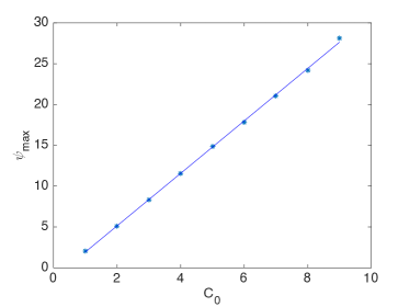
Figure 3: The maxima $\psi_{max}$ of the $L^{\infty}$ norm of the solution to the focusing NLS equation (58) for the initial data $C_{0}\mbox{sech}^{2}x$ for several values of $C_{0}=1,\ldots,9$ with a linear fit $|\psi(x,y;\epsilon)|_{max}=3.2128C_{0}-1.2864$.

with $(x_{0},y_{0})$ the point of elliptic umbilic catastrophe and $c_{0}$ a constant that depends on the initial datum. For example the first breather corresponds to the first pole at $z_{p}\simeq-2.38$ on the negative real axis of the tritronquée solution. The macroscopic feature of this behaviour is that the maximum hight of the solution is approximately $3$ times the value $b$ that is the value of $\rho(x_{0},t_{0};\epsilon=0)$ at the critical point. Furthermore the above formula for $z_{p}$ shows that the position of the lump in the $(x,t)$ plane scales like $\epsilon^{\frac{4}{5}}$. When the value $b$ is not available, one may wonder whether the maximum peak of the NLS solution scales linearly with the maximum value of the initial data. Using the same numerical approach as in [11] (we use $N=2^{14}$ Fourier modes and $N_{t}=10^{4}$ time steps), we get the $L^{\infty}$ norm of $\psi(x,y;\epsilon)$ for $\epsilon=0.1$ and for the initial data $\psi(x,0)=C_{0}\partial_{x}\mbox{sech}^{2}x$ for several values of $C_{0}$. The maxima of the $L^{\infty}$ norms are shown in Fig. 3 in dependence of $C_{0}$. They can be fitted via linear regression to the line $3.2128C_{0}-1.2864$, thus confirming that the maximum value of the solution scales linearly with the maximum value of the initial data above some threshold amplitude $C_{0}$.

We now connect the NLS breather solution (63) to the KPI lump solution (12) by observing that the expression

$$u(x,y,t)=12\left|Q\left(x-(a^{2}+3b^{2})t,2\sqrt{3}(y+2at);\frac{a}{2\sqrt{3}},\frac{b}{2}\right)\right|^{2}-3b^{2}$$ (65)

coincides with the general lump solution (12) of KPI for $\epsilon=1$. Using this connection, we make the following conjecture.

Conjecture 1.

The position of the lumps emerging from the soliton front is determined by the relation

$$z_{p}=\dfrac{c_{0}}{\epsilon^{\frac{4}{5}}}[x_{p}-(a^{2}+3b^{2})t_{p}-(x_{0}-(a^{2}+3b^{2})t_{0})+(a+\operatorname{i}\sqrt{3}b)(y_{p}+2at-y_{0}-2at_{0})],$$ (66)

where $(x_{0},y_{0})$ is the position where a singularity of the Whitham system is expected to appear at the time $t_{0}$ and $(x_{p},y_{p})$ is the position where the lump is expected to appear at the time $t_{p}$ and $c_{0}$, $a$ and $b$ are some constants.

For initial data symmetric with respect to $y\to-y$ the first lump that is appearing in the KPI solution is on the line $y=0$, thus $a=0$ and $y_{0}=y_{p}=0$ due to symmetry reasons. We conclude form (66) that the position of the first lump is expected to be given by

$$z_{p}=\dfrac{c_{0}}{\epsilon^{\frac{4}{5}}}[x_{p}-3b^{2}t_{p}-(x_{0}-3b^{2}t_{0})],$$ (67)

namely the quantity $x_{p}-3b^{2}t_{p}$ is expected to scale like $\epsilon^{\frac{4}{5}}$. We are going to verify this ansatz numerically in the next section.

4 Numerical Method

In this section we summarize the numerical methods used in the following section to solve the Cauchy problem for KPI in the small dispersion limit. We consider the evolutionary form of the KP equation (1):

$$u_{t}+uu_{x}+\epsilon^{2}u_{xxx}=-\alpha\partial_{x}^{-1}u_{yy},$$ (68)

defined on the periodic square $[-5\pi,5\pi]^{2}$, with initial condition $u(x,y,0)=u_{0}(x,y)$; here $\partial_{x}^{-1}$ is defined via its Fourier multiplier $-\mathrm{i}/k_{x}$ where $k_{x}$ is the dual Fourier variable to $x$.

For the numerical approximation of the solution $u(x,y,t)$ of equation (68), we adopt a Fourier collocation method (also known as Fourier pseudospectral method) in space coupled with a Composite Runge–Kutta method in time.

Referring to [8, 38] for a detailed overview of Fourier collocation methods and spectral methods in general, we sketch here the main features of this discretization method. The starting point of Fourier spectral methods consists in approximating the Fourier transform $\widehat{u}(k_{x},k_{y},t)$ of the solution $u(x,y,t)$, where $k_{x}$, $k_{y}$ are the dual variables to $x$, $y$, via a discrete Fourier transform for which fast algorithms exist, the fast Fourier transform (FFT). This means we approximate the rapidly decreasing initial data as a periodic (in $x$ and $y$) function. We will always work on the domain $5[-\pi,\pi]\times 5[-\pi,\pi]$ in the following. We use $N_{x}$ respectively $N_{y}$ collocation points in $x$ respectively $y$.

The discretized approximation of the KPI equation (68) can be written in the form:

$$\widehat{u}_{t}=\mathbf{L}\widehat{u}+\mathbf{N}(\widehat{u}),$$ (69)

where for the KPI equation (68), the linear and nonlinear parts $\mathbf{L}$ and $\mathbf{N}$ have the form:

$$\mathbf{L}=-\operatorname{i}\frac{k_{y}^{2}}{k_{x}}+\epsilon^{2}\operatorname{i}k_{x}^{3},$$ (70)

$$\mathbf{N}(\widehat{u})=-\frac{1}{2}\operatorname{i}k_{x}\widehat{u^{2}}.$$

The convolution in Fourier space in the nonlinear term $\mathbf{N}$ in equation (70) is computed in physical space followed by a two-dimensional FFT.

For the time discretization of equation (69) several fourth order methods were discussed in [26] for the small dispersion limit of KP. We adopt here Driscoll’s Composite Runge–Kutta method [10], which requires that the linear operator $\mathbf{L}$ of equation (70) is diagonal, which is the case here. Thus the evaluation of both positive and negative powers of $\mathbf{L}$ can be obtained with a computational cost $O(N)$.

Composite Runge–Kutta methods partition the Fourier space for the linear part of the equation into two parts, one for the low frequencies (or “slow” modes), $|\mathbf{k}|:=|(k_{x},k_{y})|<k_{\mathrm{cutoff}}$, and one for the high frequencies (or “stiff” modes), $|\mathbf{k}|\geq k_{\mathrm{cutoff}}$. Then, the Fourier components of the solution are advanced in time using different Runge–Kutta integrators for the two partitions. In particular, a third-order $L$-stable method (RK3 in the following) is used for the higher frequencies, while for the lower frequencies stiffness is not an issue and a standard explicit fourth-order method (RK4) can be used. As a result, the method is explicit, but has much better stability properties than the explicit RK4 method for which no convergence could be observed in the studied examples in [26]. Despite the use of a third order method for the high frequencies, Driscoll’s method shows in practice fourth order accuracy as shown in [26] and references therein.

In his article [10], Driscoll suggests to adopt the fourth order method for all the frequencies such that:

$$||\mathbf{L}||_{\infty}<\frac{2.8}{h},$$ (71)

where $h$ is the time-step used, in accordance with the stability region of the RK4 method, see e.g. [38]. However, in previous studies as [26] and references therein, it was observed that the method is stable only if very small time steps depending on the spatial resolution are used (obviously $h\propto 1/(N_{x}N_{y})$). For this reason, we modified condition (71) to the following:

$$||\mathbf{L}||_{\infty}<\frac{2^{-7}}{h}.$$ (72)

As a result of this change, many fewer Fourier modes of the linear part are advanced with a RK4 method than in Driscoll’s original method, but this is still preferable over a standard RK3 method (an explicit RK3 method would impose similar stability requirement as RK4, and an implicit method would make the solution of an implicit equation system necessary in each time step, which would be computationally too expensive).

Due to the very high accuracy required by our simulations, the numerical method exposed so far has been implemented in a MPI-parallel C code.

The accuracy of the solutions is controlled as in [26] in two ways: since the KPI solution for smooth initial data is known to stay smooth, its Fourier transformed must be rapidly decreasing for all time. Thus if the computational domain is chosen large enough, this must be also the case for the discrete Fourier transform. The decrease of the Fourier coefficients can thus be used to control the numerical resolution in space during the computation. If the latter is assured, the resolution in time can be controlled via conserved quantities of the KP solution as the $L^{2}$ norm or the energy, computed numerically as:

$$\|u\|_{L^{2}}^{2}=\sum_{|\mathbf{k}|=0}^{N}|\widehat{u}_{\mathbf{k}}|^{2},$$ (73)

which will be numerically time dependent due to unavoidable numerical errors. As discussed for instance in [26] the accuracy in the conservation of such quantities can be used as an indicator of the numerical accuracy.

5 Numerical solution

In this section we analyse the behaviour of the KPI solution for the initial data

$$u_{0}(x,y)=-C_{0}\partial_{x}\operatorname{sech}^{2}\sqrt{x^{2}+y^{2}}.$$ (74)

for several values of $\epsilon$ and $C_{0}$. In table 1, we report the different set-ups for the numerical simulations.

Table 1: Parameter values for the numerical experiments run (numbered by $n$) in this work.

n	$\epsilon$	$C_{0}$	$h$	grid
1	$0.02$	6	$4\cdot 10^{-5}$	$2^{15}\times 2^{15}$
2	$0.03$	6	$4\cdot 10^{-5}$	$2^{15}\times 2^{15}$
3	$0.04$	6	$8\cdot 10^{-5}$	$2^{15}\times 2^{15}$
4	$0.05$	6	$1\cdot 10^{-4}$	$2^{15}\times 2^{15}$
5	$0.06$	6	$1\cdot 10^{-4}$	$2^{14}\times 2^{14}$
6	$0.07$	6	$2\cdot 10^{-4}$	$2^{14}\times 2^{14}$
7	$0.08$	6	$1\cdot 10^{-4}$	$2^{14}\times 2^{14}$
8	$0.09$	6	$2\cdot 10^{-4}$	$2^{14}\times 2^{14}$
9	$0.10$	6	$2\cdot 10^{-4}$	$2^{14}\times 2^{14}$
10	$0.10$	4	$1\cdot 10^{-4}$	$2^{13}\times 2^{13}$
11	$0.10$	5	$1\cdot 10^{-4}$	$2^{13}\times 2^{13}$
12	$0.10$	7	$1\cdot 10^{-4}$	$2^{13}\times 2^{13}$
13	$0.10$	8	$1\cdot 10^{-4}$	$2^{13}\times 2^{13}$

The solution $u(x,y,t;\epsilon)$ starts to oscillate around the time and the location where the solution of the dKP (2) equation has its first singularity, which occurs on the positive part of the initial data. There is a second singularity that occurs slightly later on the negative part of the initial data and a dispersive shock wave develops also there. The two dispersive shock wave fronts behave quite differently in time. While in the negative front the oscillations are defocused, in the positive front the oscillations seem to be focused and the (modulated) line soliton fronts break into a number of lumps that are arranged in a lattice, as shown in Fig. 2.

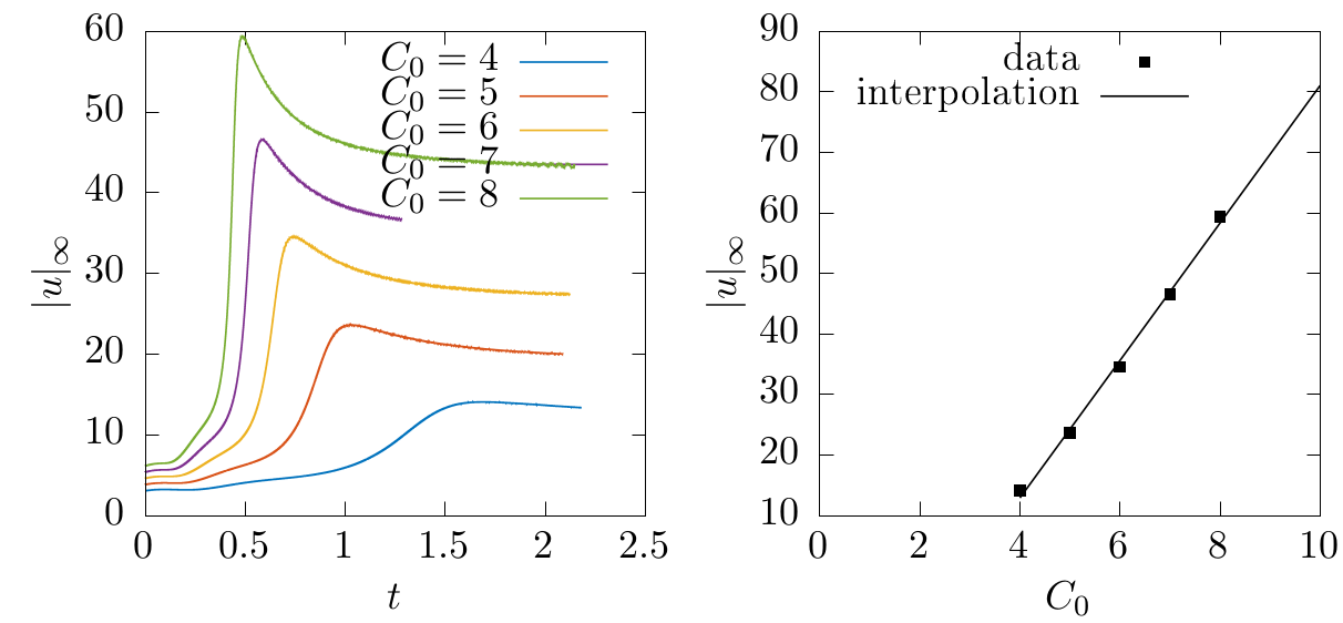
Figure 4: The $L^{\infty}$ norm the solution of the KPI equation as a function of time for $\epsilon=0.10$ and for different values of the initial amplitude. The interpolation expression is $|u|_{\infty}=10.838C_{0}-29.894$.

According to a result of [16], for small norm initial data

$$\int_{-\infty}^{\infty}\int_{-\infty}^{+\infty}\operatorname{d}y\operatorname{d}\xi\widehat{u}_{0}(\xi,y)\ll 1,$$

the solution of the KPI equations with $\epsilon=1$ does not develop lumps. Here $\widehat{u}_{0}(\xi,y)$ is the Fourier transform with respect to $x$ of the initial data. When we introduce the small $\epsilon$ parameter, such norm is of order $1/\epsilon^{2}$ and therefore it is never small. For this reason, the evolution of our initial data always develops lumps for sufficiently small $\epsilon$. However for small values of $C_{0}$, namely for $C_{0}\leq 3$ the the times required by the solution to develop the first lump were regarded as too long, and thus disregarded.

The same question as for NLS in Fig. 3 is addressed in Fig. 4 for the KPI example. We show for several values of the constant $C_{0}$ and for fixed $\epsilon=0.1$ the maximum amplitude as a function of time. The amplitude of the first lump is proportional to the initial amplitude. We then consider on the right in Fig. 4 the maximum of the $L^{\infty}$ norm in the range of time considered as a function of the maximum amplitude of the initial data $u_{0}(x,y,0)$ in (74) which is proportional to $C_{0}$. The fitting shows that $u_{max}$ is approximately $10.8$ times $C_{0}$.

In Fig. 5, one can see the formation of the first lump from the dispersive shock of KPI on the $x$-axis.

Figure 5: Solution to KPI equation for the initial data $-6\partial_{x}\operatorname{sech}^{2}\sqrt{x^{2}+y^{2}}$ along the line $y=0$ for $\epsilon=0.02$ for several values of time. The formation of the lump and its detachment from the train of oscillations can be clearly seen.

Next we consider the fitting of the first spike that emerges from the soliton front to the KP lump (12). This is shown in Fig. 6 on the $x$-axis for various values of $\epsilon$. The excellent agreement is obvious.

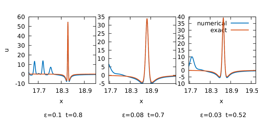
Figure 6: A comparison between the numerical solution and the lump formula (12) for four different values of $\epsilon$, at a time slightly after the lump achieves its maximum height. The maximum peak becomes narrower and higher with decreasing values of $\epsilon$.

In Fig. 7 we show the 2D-plot of the highest peak. We subtract the fitted lump solution and, as can be seen from the picture, the difference is negligible with respect to the remaining oscillations.

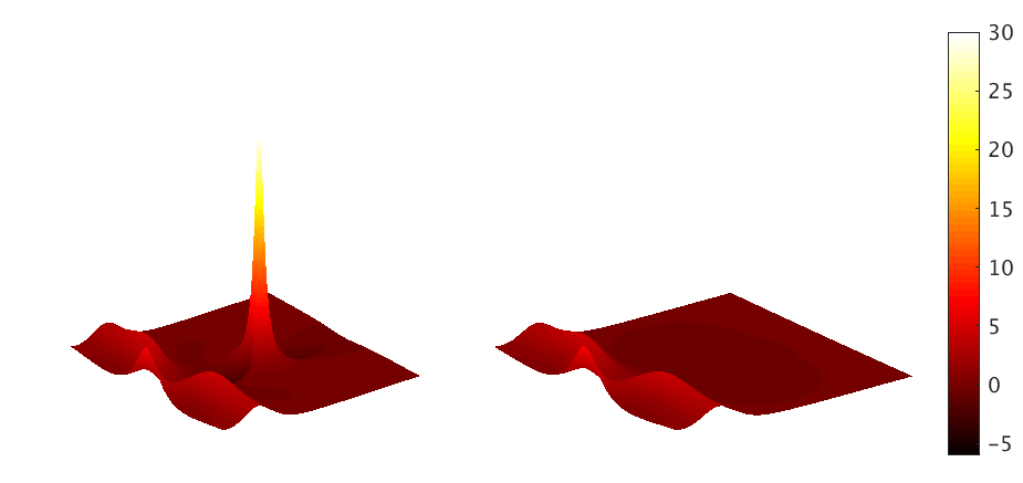
Figure 7: 2D plot of the KPI solution for $\epsilon=0.06$ and $t=0.9$. On the right picture, the maximum peak has been subtracted using the lump solution (12).

We study numerically the scaling of the lump parameters as a function of $\epsilon$ for fixed initial data. The first scaling that we consider is the $L^{\infty}$ norm $|u|_{\infty}$ as a function of $\epsilon$ (see Fig. 8). A fitting of $|u|_{\infty}$ to $c_{1}+c_{2}\epsilon^{\beta}$ with gives $c_{1}=77.9350$ $c_{2}=-191.4782$ and $\beta=0.6437$.

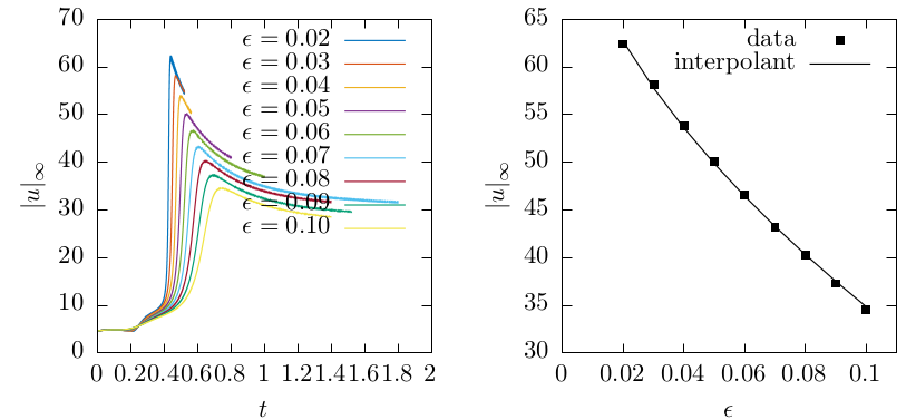
Figure 8: On the left the $L^{\infty}$ norm of the solution $u(x,y,t;\epsilon)$ as a function of time for several values of $\epsilon$. On the right a fitting of $|u|_{\infty}$ in dependence of $\epsilon$ to $c_{1}+c_{2}\epsilon^{\beta}$, which yields $c_{1}=77.9350$, $c_{2}=-191.4782$, $\beta=0.6437$.

Next we consider the dependence of the position and the time of appearance of the highest peak as a function of $\epsilon$. Since the time of the second breaking, its location and the value of the solution are not known, but all enter formula (66), it will be numerically inconclusive if they all will be identified via some fitting for $x$, $t$ and $u$ separately. Instead we just consider the combination of these values needed for (66), $x_{\text{max}}-|u|_{\text{max}}/8t_{\text{max}}$ and fit the observed values to $c_{1}+c_{2}\epsilon^{\beta}$. As shown in Fig. 9, we find $c_{1}=14.3537$, $c_{2}=6.1037$ and $\beta=0.7820$ which is compatible with the value $4/5$.

Figure 9: The value $x_{\text{max}}-|u|_{\text{max}}/8t_{\text{max}}$ as a function of $\epsilon$. A power fitting $x_{\text{max}}-|u|_{\text{max}}t_{\text{max}}/8=c_{1}+c_{2}\epsilon^{\beta}$ gives the coefficients $c_{1}=14.354$, $c_{2}=6.1037$, $\beta=0.7820$.

6 Conclusion

In this work we have presented a detailed numerical study of the long time behavior of dispersive shock waves in KPI solutions. It was shown that in the positive part of the solution, a secondary breaking of the dispersive shock wave can be observed for sufficiently long times, depending on the amplitude of the initial data. At this secondary breaking, the parabolic shock fronts develop a cusp from which modulated lump solutions emerge. We have justified this behaviour with the observation that the Whitham modulation equations near the solitonic front are not hyperbolic. The scaling of the maximum of the solution is linear with respect to the maximum amplitude of the initial data, and for the specific initial data considered, this scaling coefficient turns out to be about 10. Regarding the scaling of $x$ and $t$ as a function of $\epsilon$, the same scalings are observed as in the case of the semiclassical limit of focusing NLS.

It would be interesting to identify the values of the break-up point $(x_{0},y_{0},t_{0})$ for given initial data. A way to obtain this information would be to solve the Whitham equations and to determine the point where their solutions develop a cusp for given initial data. A detailed study of the Whitham equations could also give an indication on how to make the above conjecture more precise, and how to prove it eventually. Finally a more mathematical goal is the study of the integrability and Hamiltonian structure of the Whitham modulation equation as defined in [13], [14]. This will be the subject of further work.

Funding T.G. acknowledges the support by the Leverhulme Trust Research Fellowship RF-2015-442.

Acknowledgements We thank Miguel Onorato, Peter Miller, Karima Khusnutdinova for valuable discussions during the preparation of this manuscript.

References

- [1] M.J. Ablowitz, A. Demirci, Yi-Ping Ma, Dispersive shock waves in the Kadomtsev–Petviashvili and Two Dimensional Benjamin–Ono equations. arXiv:1507.08207.
- [2] M.J.Ablowitz, P.A.Clarkson 1991 Solitons, nonlinear evolution equations and inverse scattering. Cambridge, UK: Cambridge University Press.
- [3] M. Bertola, A. Tovbis, Universality for the focusing nonlinear Schr dinger equation at the gradient catastrophe point: rational breathers and poles of the tritronquée solution to Painlevé I. Comm. Pure Appl. Math. 66 (2013), no. 5, 678 - 752.
- [4] G.Biondini, G.El, M.Hoefer, P.Miller, Dispersive hydrodynamics: preface. Phys. D 333 (2016), 1?5.
- [5] M.J. Ablowitz, G. Biondini, Qiao Wang, Whitham modulation theory for the Kadomtsev-Petviashvili equation. Proc. A. 473 (2017), no. 2204, 20160695, 23 pp.
- [6] M. Boiti, F. Pempinelli, A.K. Pogrebkov, and M.C. Polivanov, Inverse Problems 8 (1992), 331.
- [7] J. Bourgain, On the Cauchy problem for the Kadomtsev–Petviashvili equation, Geom. Funct. Anal. 3 (1993), 315-341.
- [8] C. Canuto, M.Y. Hussaini, A. Quarteroni and T. Zhang, Spectral Methods, Vol. 1, Springer (2006)
- [9] V.S. Dryuma, Analytic solutions of the two-dimensional Korteweg–de Vries equation, Pis’ma ZhETF 19 (1974) 753-757.
- [10] T. Driscoll, A composite Runge-Kutta Method for the spectral Solution of semilinear PDEs, Journal of Computational Physics, 182 (2002), pp. 357 - 367.
- [11] B. Dubrovin, T. Grava and C. Klein, Numerical Study of breakup in generalized Korteweg–de Vries and Kawahara equations, SIAM J. Appl. Math. 71 (2011) 983-1008.
- [12] G. A. El, A. M. Kamchatnov, V. V. Khodorovskii, E. S. Annibale, and A. Gammal, Two-dimensional supersonic nonlinear Schrödinger equation flow past an extended obstacle, Phys. Rev. E 80 (2009) 046317.
- [13] E. V. Ferapontov and K. R. Khusnutdinova, The Haantjes tensor and double waves for multi- dimensional systems of hydrodynamic type: a necessary condition for integrability, Proc. R. Soc. Lond. A, 462, (2006) 1197 - 1219.
- [14] E. V. Ferapontov, P. Lorenzoni, A.Savoldi, Hamiltonian operators of Dubrovin-Novikov type in 2D. Lett. Math. Phys. 105 (2015), no. 3, 341 - 377.
- [15] A.S. Fokas, M.J. Ablowitz, On the inverse scattering of the time-dependent Schr dinger equation and the associated Kadomtsev–Petviashvili equation. Stud. Appl. Math. 69 (1983), no. 3, 211-228.
- [16] A.S. Fokas and L.Y. Sung, The Cauchy problem for the Kadomtsev–Petviashvili-I equation without the zero mass constraint, Math. Proc. Camb. Phil. Soc. (1999), 125, 113.
- [17] T. Grava and C. Klein, Numerical solution of the small dispersion limit of Korteweg de Vries and Whitham equations, Comm. Pure Appl. Math. 60(11) (2007) 1623-1664.
- [18] T. Grava, C. Klein and J. Eggers, Shock formation in the dispersionless Kadomtsev–Petviashvili equation, Nonlinearity 29 1384-1416 (2016)
- [19] A. V. Gurevich and L. P. Pitaevskii, Non stationary structure of collisionless shock waves, JETP Letters, 17, 193-195 (1973)
- [20] M. A. Hoefer and B. Ilan, Theory of two-dimensional oblique dispersive shock waves in supersonic flow of a superfluid, Phys. Rev. A 80 (2009), 061601(R).
- [21] E. Infeld and G. Rowlands, Nonlinear Waves, Solitons and Chaos (Cambridge University Press, Cambridge, 1992).
- [22] B. B. Kadomtsev and V. I. Petviashvili, On the stability of solitary waves in weakly dispersive media, Sov. Phys. Dokl. 15 (1970), 539.
- [23] S. Kamvissis, K.D. T.-R McLaughlin, P.D. Miller, Semiclassical soliton ensembles for the focusing nonlinear Schr dinger equation. Annals of Mathematics Studies, 154. Princeton University Press, Princeton, NJ, 2003.
- [24] C. Klein and K. Roidot, Numerical study of shock formation in the dispersionless Kadomtsev–Petviashvili equation and dispersive regularizations, Physica D 265 (2013) 1–25.
- [25] C. Klein and J.-C. Saut, Numerical study of blow up and stability of solutions of generalized Kadomtsev–Petviashvili equations, J. Nonl. Sci. 22 (5) (2012) 763-811.
- [26] C. Klein and K. Roidot, Fourth order time-stepping for Kadomtsev–Petviashvili and Davey–Stewartson equations, SIAM J. Sci. Comput. 33(6) (2011) 3333-3356.
- [27] C. Klein, C. Sparber and P. Markowich, Numerical study of oscillatory regimes in the Kadomtsev–Petviashvili equation, J. Nonl. Sci. 17(5) (2007) 429-470.
- [28] D.F. Lawden, Elliptic functions and applications. Applied Mathematical Sciences, 80. Springer-Verlag, New York, 1989. xiv+334 pp. ISBN: 0-387-96965-9.
- [29] I.M. Krichever, The averaging method for two-dimensional ”integrable” equations. Funct. Anal. Appl. 22 (1988), no. 3, 200 - 213.
- [30] C. Lin, E. Reissner, and H.S. Tsien, On two-dimensional non-steady motion of a slender body in a compressible fluid. J. Math. Physics. 27 (1948) 220-231
- [31] S.V. Manakov and P.M. Santini, On the solutions of the dKP equation: the nonlinear Riemann–Hilbert problem, longtime behaviour, implicit solutions and wave breaking, Nonlinearity 41 (2008), 1.
- [32] A.A. Minzoni, N.F.Smyth, Evolution of lump solutions for the KP equation. Wave Motion 24 (1996), no. 3, 291 - 305.
- [33] L. Molinet, J.C. Saut, N. Tzvetkov, Global well-posedness for the KP-I equation. Math. Ann. 324 (2002), no. 2, 255-275.
- [34] D. E. Pelinovsky, C. Sulem, Eigenfunctions and Eigenvalues for a Scalar Riemann–Hilbert Problem Associated to Inverse Scattering, Commun. Math. Phys. (2000) 208, 713–760.
- [35] Ratliff, Daniel J.(4-SUR); Bridges, Thomas J.(4-SUR) Whitham modulation equations, coalescing characteristics, and dispersive Boussinesq dynamics. Phys. D 333 (2016), 107 - 116.
- [36] F. Rousset, N. Tzvetkov, Stability and Instability of the KDV Solitary Wave Under the KP-I Flow, Comm. Math. Phys. 313(1) (2012) 155 - 173.
- [37] A. Rozanova, The Khokhlov-Zabolotskaya-Kuznetsov equation. C. R. Math. Acad. Sci. Paris 344 (2007), no. 5, 337-342.
- [38] L.N. Trefethen, Spectral Methods in Matlab. SIAM, Philadelphia (2000)
- [39] S. Trillo, M. Klein, G.F. Clauss, M.Onorato, Observation of dispersive shock waves developing from initial depressions in shallow water. Phys. D 333 (2016), 276 - 284.
- [40] G.B. Whitham, G. B. Linear and nonlinear waves. Reprint of the 1974 original. Pure and Applied Mathematics (New York). A Wiley-Interscience Publication. John Wiley and Sons, Inc., New York, 1999. xviii+636 pp. ISBN: 0-471-35942-4 35-01
- [41] E.A. Zabolotskaya and R.V. Khokhlov, Quasi-plane waves in the nonlinear acoustics of confined beams, Sov. Phys. Acoustics 15 (1969), 35–40.
- [42] Zakharov, V.E.: Instability and nonlinear oscillations of solitons. JETP Lett. 22, 172 - 173 (1975)