Provable Alternating Gradient Descent for Non-negative Matrix Factorization with Strong Correlations

Abstract

Non-negative matrix factorization is a basic tool for decomposing data into the feature and weight matrices under non-negativity constraints, and in practice is often solved in the alternating minimization framework. However, it is unclear whether such algorithms can recover the ground-truth feature matrix when the weights for different features are highly correlated, which is common in applications. This paper proposes a simple and natural alternating gradient descent based algorithm, and shows that with a mild initialization it provably recovers the ground-truth in the presence of strong correlations. In most interesting cases, the correlation can be in the same order as the highest possible. Our analysis also reveals its several favorable features including robustness to noise. We complement our theoretical results with empirical studies on semi-synthetic datasets, demonstrating its advantage over several popular methods in recovering the ground-truth.

1 Introduction

Non-negative matrix factorization (NMF) is an important tool in data analysis and is widely used in image processing, text mining, and hyperspectral imaging (e.g., (Lee & Seung, 1997; Blei et al., 2003; Yang & Leskovec, 2013)). Given a set of observations $\mathbb{Y}=\{y^{(1)},y^{(2)},\ldots,y^{(n)}\}$, the goal of NMF is to find a feature matrix $\mathbb{A}=\{a_{1},a_{2},\ldots,a_{D}\}$ and a non-negative weight matrix $\mathbb{X}=\{x^{(1)},x^{(2)},\ldots,x^{(n)}\}$ such that $y^{(i)}\approx\mathbb{A}x^{(i)}$ for any $i$, or $\mathbb{Y}\approx\mathbb{A}\mathbb{X}$ for short. The intuition of NMF is to write each data point as a non-negative combination of the features. By doing so, one can avoid cancellation of different features and improve interpretability by thinking of each $x^{(i)}$ as a (unnormalized) probability distribution over the features. It is also observed empirically that the non-negativity constraint on the coefficients can lead to better features and improved downstream performance of the learned features.

Unlike the counterpart which factorizes $\mathbb{Y}\approx\mathbb{A}\mathbb{X}$ without assuming non-negativity of $\mathbb{X}$, NMF is usually much harder to solve, and can even by NP-hard in the worse case (Arora et al., 2012b). This explains why, despite all the practical success, NMF largely remains a mystery in theory. Moreover, many of the theoretical results for NMF were based on very technical tools such has algebraic geometry (e.g., (Arora et al., 2012b)) or tensor decomposition (e.g. (Anandkumar et al., 2012)), which undermine their applicability in practice. Arguably, the most widely used algorithms for NMF use the alternative minimization scheme: In each iteration, the algorithm alternatively keeps $\mathbb{A}$ or $\mathbb{X}$ as fixed and tries to minimize some distance between $\mathbb{Y}$ and $\mathbb{A}\mathbb{X}$. Algorithms in this framework, such as multiplicative update (Lee & Seung, 2001) and alternative non-negative least square (Kim & Park, 2008), usually perform well on real world data. However, alternative minimization algorithms are usually notoriously difficult to analyze. This problem is poorly understood, with only a few provable guarantees known (Awasthi & Risteski, 2015; Li et al., 2016). Most importantly, these results are only for the case when the coordinates of the weights are from essentially independent distributions, while in practice they are known to be correlated, for example, in correlated topic models (Blei & Lafferty, 2006). As far as we know, there exists no rigorous analysis of practical algorithms for the case with strong correlations.

In this paper, we provide a theoretical analysis of a natural algorithm AND (Alternative Non-negative gradient Descent) that belongs to the practical framework, and show that it probably recovers the ground-truth given a mild initialization. It works under general conditions on the feature matrix and the weights, in particular, allowing strong correlations. It also has multiple favorable features that are unique to its success. We further complement our theoretical analysis by experiments on semi-synthetic data, demonstrating that the algorithm converges faster to the ground-truth than several existing practical algorithms, and providing positive support for some of the unique features of our algorithm. Our contributions are detailed below.

1.1 Contributions

In this paper, we assume a generative model of the data points, given the ground-truth feature matrix $\mathbb{A}^{*}$. In each round, we are given $y=\mathbb{A}^{*}x$, where $x$ is sampled i.i.d. from some unknown distribution $\mu$ and the goal is to recover the ground-truth feature matrix $\mathbb{A}^{*}$. We give an algorithm named AND that starts from a mild initialization matrix and provably converges to $\mathbb{A}^{*}$ in polynomial time. We also justify the convergence through a sequence of experiments. Our algorithm has the following favorable characteristics.

1.1.1 Simple Gradient Descent Algorithm

The algorithm AND runs in stages and keeps a working matrix $\mathbb{A}^{(t)}$ in each stage. At the $t$-th iteration in a stage, after getting one sample $y$, it performs the following:

(Decode) $$z=\phi_{\alpha}\left((\mathbb{A}^{(0)})^{\dagger}y\right),$$

(Update) $$\mathbb{A}^{(t+1)}=\mathbb{A}^{(t)}+\eta\left(yz^{\top}-\mathbb{A}^{(t)}zz^{\top}\right),$$

where $\alpha$ is a threshold parameter,

$$\phi_{\alpha}(x)=\left\{\begin{array}[]{ll}x&\mbox{if $x\geq\alpha$},\\ 0&\mbox{otherwise},\end{array}\right.$$

$(\mathbb{A}^{(0)})^{\dagger}$ is the Moore-Penrose pesudo-inverse of $\mathbb{A}^{(0)}$, and $\eta$ is the update step size. The decode step aims at recovering the corresponding weight for the data point, and the update step uses the decoded weight to update the feature matrix. The final working matrix at one stage will be used as the $\mathbb{A}^{(0)}$ in the next stage. See Algorithm 1 for the details.

At a high level, our update step to the feature matrix can be thought of as a gradient descent version of alternative non-negative least square (Kim & Park, 2008), which at each iteration alternatively minimizes $L(\mathbb{A},\mathbb{Z})=\|\mathbb{Y}-\mathbb{A}\mathbb{Z}\|_{F}^{2}$ by fixing $\mathbb{A}$ or $\mathbb{Z}$. Our algorithm, instead of performing an complete minimization, performs only a stochastic gradient descent step on the feature matrix. To see this, consider one data point $y$ and consider minimizing $L(\mathbb{A},z)=\|y-\mathbb{A}z\|_{F}^{2}$ with $z$ fixed. Then the gradient of $\mathbb{A}$ is just $-\nabla L(\mathbb{A})=(y-\mathbb{A}z)z^{\top}$, which is exactly the update of our feature matrix in each iteration.

As to the decode step, when $\alpha=0$, our decoding can be regarded as a one-shot approach minimizing $\|\mathbb{Y}-\mathbb{A}\mathbb{Z}\|_{F}^{2}$ restricted to $\mathbb{Z}\geq 0$. Indeed, if for example projected gradient descent is used to minimize $\|\mathbb{Y}-\mathbb{A}\mathbb{Z}\|_{F}^{2}$, then the projection step is exactly applying $\phi_{\alpha}$ to $\mathbb{Z}$ with $\alpha=0$. A key ingredient of our algorithm is choosing $\alpha$ to be larger than zero and then decreasing it, which allows us to outperform the standard algorithms.

Perhaps worth noting, our decoding only uses $\mathbb{A}^{(0)}$. Ideally, we would like to use $(\mathbb{A}^{(t)})^{\dagger}$ as the decoding matrix in each iteration. However, such decoding method requires computing the pseudo-inverse of $\mathbb{A}^{(t)}$ at every step, which is extremely slow. Instead, we divide the algorithm into stages and in each stage, we only use the starting matrix in the decoding, thus the pseudo-inverse only needs to be computed once per stage and can be used across all iterations inside. We can show that our algorithm converges in polylogarithmic many stages, thus gives us to a much better running time. These are made clear when we formally present the algorithm in Section 4 and the theorems in Section 5 and 6.

1.1.2 Handling strong correlations

The most notable property of AND is that it can provably deal with highly correlated distribution $\mu$ on the weight $x$, meaning that the coordinates of $x$ can have very strong correlations with each other. This is important since such correlated $x$ naturally shows up in practice. For example, when a document contains the topic “machine learning”, it is more likely to contain the topic “computer science” than “geography” (Blei & Lafferty, 2006).

Most of the previous theoretical approaches for analyzing alternating between decoding and encoding, such as (Awasthi & Risteski, 2015; Li et al., 2016; Arora et al., 2015), require the coordinates of $x$ to be pairwise-independent, or almost pairwise-independent (meaning $\mathbb{E}_{\mu}[x_{i}x_{j}]\approx\mathbb{E}_{\mu}[x_{i}]\mathbb{E}_{\mu}[x_{j}]$). In this paper, we show that algorithm AND can recover $\mathbb{A}^{*}$ even when the coordinates are highly correlated. As one implication of our result, when the sparsity of $x$ is $O(1)$ and each entry of $x$ is in $\{0,1\}$, AND can recover $\mathbb{A}^{*}$ even if each $\mathbb{E}_{\mu}[x_{i}x_{j}]=\Omega(\min\{\mathbb{E}_{\mu}[x_{i}],\mathbb{E}_{\mu}[x_{j}]\})$, matching (up to constant) the highest correlation possible. Moreover, we do not assume any prior knowledge about the distribution $\mu$, and the result also extends to general sparsities as well.

1.1.3 Pseudo-inverse decoding

One of the feature of our algorithm is to use Moore-Penrose pesudo-inverse in decoding. Inverse decoding was also used in (Li et al., 2016; Arora et al., 2015, 2016). However, their algorithms require carefully finding an inverse such that certain norm is minimized, which is not as efficient as the vanilla Moore-Penrose pesudo-inverse. It was also observed in (Arora et al., 2016) that Moore-Penrose pesudo-inverse works equally well in practice, but the experiment was done only when $\mathbb{A}=\mathbb{A}^{*}$. In this paper, we show that Moore-Penrose pesudo-inverse also works well when $\mathbb{A}\not=\mathbb{A}^{*}$, both theoretically and empirically.

1.1.4 Thresholding at different $\alpha$

Thresholding at a value $\alpha>0$ is a common trick used in many algorithms. However, many of them still only consider a fixed $\alpha$ throughout the entire algorithm. Our contribution is a new method of thresholding that first sets $\alpha$ to be high, and gradually decreases $\alpha$ as the algorithm goes. Our analysis naturally provides the explicit rate at which we decrease $\alpha$, and shows that our algorithm, following this scheme, can provably converge to the ground-truth $\mathbb{A}^{*}$ in polynomial time. Moreover, we also provide experimental support for these choices.

1.1.5 Robustness to noise

We further show that the algorithm is robust to noise. In particular, we consider the model $y=\mathbb{A}^{*}x+\zeta$, where $\zeta$ is the noise. The algorithm can tolerate a general family of noise with bounded moments; we present in the main body the result for a simplified case with Gaussian noise and provide the general result in the appendix. The algorithm can recover the ground-truth matrix up to a small blow-up factor times the noise level in each example, when the ground-truth has a good condition number. This robustness is also supported by our experiments.

2 Related Work

Practical algorithms. Non-negative matrix factorization has a rich empirical history, starting with the practical algorithms of (Lee & Seung, 1997, 1999, 2001). It has been widely used in applications and there exist various methods for NMF, e.g., (Kim & Park, 2008; Lee & Seung, 2001; Cichocki et al., 2007; Ding et al., 2013, 2014). However, they do not have provable recovery guarantees.

Theoretical analysis. For theoretical analysis, (Arora et al., 2012b) provided a fixed-parameter tractable algorithm for NMF using algebraic equations. They also provided matching hardness results: namely they show there is no algorithm running in time $(mW)^{o(D)}$ unless there is a sub-exponential running time algorithm for 3-SAT. (Arora et al., 2012b) also studied NMF under separability assumptions about the features, and (Bhattacharyya et al., 2016) studied NMF under related assumptions. The most related work is (Li et al., 2016), which analyzed an alternating minimization type algorithm. However, the result only holds with strong assumptions about the distribution of the weight $x$, in particular, with the assumption that the coordinates of $x$ are independent.

Topic modeling. Topic modeling is a popular generative model for text data (Blei et al., 2003; Blei, 2012). Usually, the model results in NMF type optimization problems with $\|x\|_{1}=1$, and a popular heuristic is variational inference, which can be regarded as alternating minimization in KL-divergence. Recently, there is a line of theoretical work analyzing tensor decomposition (Arora et al., 2012a, 2013; Anandkumar et al., 2013) or combinatorial methods (Awasthi & Risteski, 2015). These either need strong structural assumptions on the word-topic matrix $\mathbb{A}^{*}$, or need to know the distribution of the weight $x$, which is usually infeasible in applications.

3 Problem and Definitions

We use $\|\mathbb{M}\|_{2}$ to denote the 2-norm of a matrix $\mathbb{M}$. $\|x\|_{1}$ is the 1-norm of a vector $x$. We use $[\mathbb{M}]_{i}$ to denote the i-th row and $[\mathbb{M}]^{i}$ to denote the $i$-th column of a matrix $\mathbb{M}$. $\sigma_{\max}(\mathbb{M})(\sigma_{\min}(\mathbb{M}))$ stands for the maximum (minimal) singular value of $\mathbb{M}$, respectively. We consider a generative model for non-negative matrix factorization, where the data $y$ is generated from

$$y=\mathbb{A}^{*}x,\quad\mathbb{A}^{*}\in\mathbb{R}^{W\times D}$$

where $\mathbb{A}^{*}$ is the ground-truth feature matrix, and $x$ is a non-negative random vector drawn from an unknown distribution $\mu$. The goal is to recover the ground-truth $\mathbb{A}^{*}$ from i.i.d. samples of the observation $y$.

Since the general non-negative matrix factorization is NP-hard (Arora et al., 2012b), some assumptions on the distribution of $x$ need to be made. In this paper, we would like to allow distributions as general as possible, especially those with strong correlations. Therefore, we introduce the following notion called $(r,k,m,\lambda)$-general correlation conditions (GCC) for the distribution of $x$.

Definition 1 (General Correlation Conditions, GCC).

Let $\mathbb{\Delta}:=\mathbb{E}[xx^{\top}]$ denote the second moment matrix.

1. $\|x\|_{1}\leq r$ and $x_{i}\in[0,1],\forall i\in[D]$.

2. $\mathbb{\Delta}_{i,i}\leq\frac{2k}{D},\forall i\in[D]$.

3. $\mathbb{\Delta}_{i,j}\leq\frac{m}{D^{2}},\forall i\neq j\in[D]$.

4. $\mathbb{\Delta}\succeq\frac{k}{D}\lambda\mathbb{I}$.

The first condition regularizes the sparsity of $x$. The second condition regularizes each coordinate of $x_{i}$ so that there is no $x_{i}$ being large too often. The third condition regularizes the maximum pairwise correlation between $x_{i}$ and $x_{j}$. The fourth condition always holds for $\lambda=0$ since $\mathbb{E}[xx^{\top}]$ is a PSD matrix. Later we will assume this condition holds for some $\lambda>0$ to avoid degenerate cases. Note that we put the weight $k/D$ before $\lambda$ such that $\lambda$ defined in this way will be a positive constant in many interesting examples discussed below.

To get a sense of what are the ranges of $k,m,$ and $\lambda$ given sparsity $r$, we consider the following most commonly studied non-negative random variables.

Proposition 1 (Examples of GCC).

1. If $x$ is chosen uniformly over $s$-sparse random vectors with $\{0,1\}$ entries, then $k=r=s$, $m=s^{2}$ and $\lambda=1-\frac{1}{s}$.

2. If $x$ is uniformly chosen from Dirichlet distribution with parameter $\alpha_{i}=\frac{s}{D}$, then $r=k=1$ and $m=\frac{1}{sD}$ with $\lambda=1-\frac{1}{s}$.

For these examples, the result in this paper shows that we can recover $\mathbb{A}^{*}$ for aforementioned random variables $x$ as long as $s=O(D^{1/6})$. In general, there is a wide range of parameters $(r,k,m,\lambda)$ such that learning $\mathbb{A}^{*}$ is doable with polynomially many samples of $y$ and in polynomial time.

However, just the GCC condition is not enough for recovering $\mathbb{A}^{*}$. We will also need a mild initialization.

Definition 2 ($\ell$-initialization).

The initial matrix $\mathbb{A}_{0}$ satisfies for some $\ell\in[0,1)$,

1. $\mathbb{A}_{0}=\mathbb{A}^{*}(\mathbb{\Sigma}+\mathbb{E})$, for some diagonal matrix $\mathbb{\Sigma}$ and off-diagonal matrix $\mathbb{E}$.

2. $\|\mathbb{E}\|_{2}\leq\ell$, $\|\mathbb{\Sigma}-\mathbb{I}\|_{2}\leq\frac{1}{4}$.

The condition means that the initialization is not too far away from the ground-truth $\mathbb{A}^{*}$. For any $i\in[D]$, the $i$-th column $[\mathbb{A}_{0}]^{i}=\mathbb{\Sigma}_{i,i}[\mathbb{A}^{*}]^{i}+\sum_{j\neq i}\mathbb{E}_{j,i}[\mathbb{A}^{*}]^{j}$. So the condition means that each feature $[\mathbb{A}_{0}]^{i}$ has a large fraction of the ground-truth feature $[\mathbb{A}^{*}]^{i}$ and a small fraction of the other features. $\mathbb{\Sigma}$ can be regarded as the magnitude of the component from the ground-truth in the initialization, while $\mathbb{E}$ can be regarded as the magnitude of the error terms. In particular, when $\mathbb{\Sigma}=\mathbb{I}$ and $\mathbb{E}=0$, we have $\mathbb{A}_{0}=\mathbb{A}^{*}$. The initialization allows $\mathbb{\Sigma}$ to be a constant away from $\mathbb{I}$, and the error term $\mathbb{E}$ to be $\ell$ (in our theorems $\ell$ can be as large as a constant).

In practice, such an initialization is typically achieved by setting the columns of $\mathbb{A}_{0}$ to reasonable “pure” data points that contain one major feature and a small fraction of some others (e.g. (lda, 2016; Awasthi & Risteski, 2015)).

4 Algorithm

Algorithm 1 Alternating Non-negative gradient Descent (AND)

0:  Threshold values $\{\alpha_{0},\alpha_{1},\ldots,\alpha_{s}\}$, $T$, $\mathbb{A}_{0}$

1:  $\mathbb{A}^{(0)}\leftarrow\mathbb{A}_{0}$

2:  for $j=0,1,\ldots,s$ do

3:     for $t=0,1,\ldots,T$ do

4:        On getting sample $y^{(t)}$, do:

5:        $z^{(t)}\leftarrow\phi_{\alpha_{j}}\left((\mathbb{A}^{(0)})^{\dagger}y^{(t)}\right)$

6:        $\mathbb{A}^{(t+1)}\leftarrow\mathbb{A}^{(t)}+\eta\left(y^{(t)}-\mathbb{A}^{(t)}z^{(t)}\right)(z^{(t)})^{\top}$

7:     end for

8:     $\mathbb{A}^{(0)}\leftarrow\mathbb{A}^{(T+1)}$

9:  end for

9:  $\mathbb{A}\leftarrow\mathbb{A}^{(T+1)}$

The algorithm is formally describe in Algorithm 1. It runs in $s$ stages, and in the $j$-th stage, uses the same threshold $\alpha_{j}$ and the same matrix $\mathbb{A}^{(0)}$ for decoding, where $\mathbb{A}^{(0)}$ is either the input initialization matrix or the working matrix obtained at the end of the last stage. Each stage consists of $T$ iterations, and each iteration decodes one data point and uses the decoded result to update the working matrix. It can use a batch of data points instead of one data point, and our analysis still holds.

By running in stages, we save most of the cost of computing $(\mathbb{A}^{(0)})^{\dagger}$, as our results show that only polylogarithmic stages are needed. For the simple case where $x\in\{0,1\}^{D}$, the algorithm can use the same threshold value $\alpha=1/4$ for all stages (see Theorem 1), while for the general case, it needs decreasing threshold values across the stages (see Theorem 4). Our analysis provides the hint for setting the threshold; see the discussion after Theorem 4, and Section 7 for how to set the threshold in practice.

5 Result for A Simplified Case

In this section, we consider the following simplified case:

$$y=\mathbb{A}^{*}x,~{}~{}x\in\{0,1\}^{D}.$$ (5.1)

That is, the weight coordinates $x_{i}$’s are binary.

Theorem 1 (Main, binary).

For the generative model (5.1), there exists $\ell=\Omega(1)$ such that for every $(r,k,m,\lambda)$-GCC $x$ and every $\epsilon>0$, Algorithm AND with $T=\textsf{poly}(D,\frac{1}{\epsilon}),\eta=\frac{1}{\textsf{poly}(D,\frac{1}{\epsilon})}$, $\{\alpha_{i}\}_{i=1}^{s}=\{\frac{1}{4}\}_{i=1}^{s}$ for $s=\textsf{polylog}(D,\frac{1}{\epsilon})$ and an $\ell$ initialization matrix $\mathbb{A}_{0}$, outputs a matrix $\mathbb{A}$ such that there exists a diagonal matrix $\mathbb{\Sigma}\succeq\frac{1}{2}\mathbb{I}$ with $\|\mathbb{A}-\mathbb{A}^{*}\mathbb{\Sigma}\|_{2}\leq\epsilon$ using $\textsf{poly}(D,\frac{1}{\epsilon})$ samples and iterations, as long as

$$m=O\left(\frac{kD\lambda^{4}}{r^{5}}\right).$$

Therefore, our algorithm recovers the ground-truth $\mathbb{A}^{*}$ up to scaling. The scaling in unavoidable since there is no assumption on $\mathbb{A}^{*}$, so we cannot, for example, distinguish $\mathbb{A}^{*}$ from $2\mathbb{A}^{*}$. Indeed, if we in addition assume each column of $\mathbb{A}^{*}$ has norm $1$ as typical in applications, then we can recover $\mathbb{A}^{*}$ directly. In particular, by normalizing each column of $\mathbb{A}$ to have norm 1, we can guarantee that $\|\mathbb{A}-\mathbb{A}^{*}\|_{2}\leq O(\epsilon).$

In many interesting applications (for example, those in Proposition 1), $k,r,\lambda$ are constants. The theorem implies that the algorithm can recover $\mathbb{A}^{*}$ even when $m=O(D)$. In this case, $\mathbb{E}_{\mu}[x_{i}x_{j}]$ can be as large as $O(1/D)$, the same order as $\min\{\mathbb{E}_{\mu}[x_{i}],\mathbb{E}_{\mu}[x_{j}]\}$, which is the highest possible correlation.

5.1 Intuition

The intuition comes from assuming that we have the “correct decoding”, that is, suppose magically for every $y^{(t)}$, our decoding $z^{(t)}=\phi_{\alpha_{j}}(\mathbb{A}^{\dagger}y^{(t)})=x^{(t)}$. Here and in this subsection, $\mathbb{A}$ is a shorthand for $\mathbb{A}^{(0)}$. The gradient descent is then $\mathbb{A}^{(t+1)}=\mathbb{A}^{(t)}+\eta(y^{(t)}-\mathbb{A}^{(t)}x^{(t)})(x^{(t)})^{\top}$. Subtracting $\mathbb{A}^{*}$ on both side, we will get

$$(\mathbb{A}^{(t+1)}-\mathbb{A}^{*})=(\mathbb{A}^{(t)}-\mathbb{A}^{*})(\mathbb{I}-\eta x^{(t)}(x^{(t)})^{\top})$$

Since $x^{(t)}(x^{(t)})^{\top}$ is positive semidefinite, as long as $\mathbb{E}[x^{(t)}(x^{(t)})^{\top}]\succ 0$ and $\eta$ is sufficiently small, $\mathbb{A}^{(t)}$ will converge to $\mathbb{A}^{*}$ eventually.

However, this simple argument does not work when $\mathbb{A}\not=\mathbb{A}^{*}$ and thus we do not have the correct decoding. For example, if we just let the decoding be $\tilde{z}^{(t)}=\mathbb{A}^{\dagger}y^{(t)}$, we will have $y^{(t)}-\mathbb{A}\tilde{z}^{(t)}=y^{(t)}-\mathbb{A}^{\dagger}\mathbb{A}y^{(t)}=(\mathbb{I}-\mathbb{A}^{\dagger}\mathbb{A})\mathbb{A}^{*}x^{(t)}$. Thus, using this decoding, the algorithm can never make any progress once $\mathbb{A}$ and $\mathbb{A}^{*}$ are in the same subspace.

The most important piece of our proof is to show that after thresholding, $z^{(t)}=\phi_{\alpha}(\mathbb{A}^{\dagger}y^{(t)})$ is much closer to $x^{(t)}$ than $\tilde{z}^{(t)}$. Since $\mathbb{A}$ and $\mathbb{A}^{*}$ are in the same subspace, inspired by (Li et al., 2016) we can write $\mathbb{A}^{*}$ as $\mathbb{A}(\mathbb{\Sigma}+\mathbb{E})$ for a diagonal matrix $\mathbb{\Sigma}$ and an off-diagonal matrix $\mathbb{E}$, and thus the decoding becomes $z^{(t)}=\phi_{\alpha}(\mathbb{\Sigma}x^{(t)}+\mathbb{E}x^{(t)})$. Let us focus on one coordinate of $z^{(t)}$, that is, $z^{(t)}_{i}=\phi_{\alpha}(\mathbb{\Sigma}_{i,i}x^{(t)}_{i}+\mathbb{E}_{i}x^{(t)})$, where $\mathbb{E}_{i}$ is the $i$-th row of $\mathbb{E}_{i}$. The term $\mathbb{\Sigma}_{i,i}x^{(t)}_{i}$ is a nice term since it is just a rescaling of $x^{(t)}_{i}$, while $\mathbb{E}_{i}x^{(t)}$ mixes different coordinates of $x^{(t)}$. For simplicity, we just assume for now that $x_{i}^{(t)}\in\{0,1\}$ and $\mathbb{\Sigma}_{i,i}=1$. In our proof, we will show that the threshold will remove a large fraction of $\mathbb{E}_{i}x^{(t)}$ when $x^{(t)}_{i}=0$, and keep a large fraction of $\mathbb{\Sigma}_{i,i}x^{(t)}_{i}$ when $x^{(t)}_{i}=1$. Thus, our decoding is much more accurate than without thresholding. To show this, we maintain a crucial property that for our decoding matrix, we always have $\|\mathbb{E}_{i}\|_{2}=O(1)$. Assuming this, we first consider two extreme cases of $\mathbb{E}_{i}$.

1. Ultra dense: all coordinates of $\mathbb{E}_{i}$ are in the order of $\frac{1}{\sqrt{d}}$. Since the sparsity of $x^{(t)}$ is $r$, as long as $r=o(\sqrt{d})\alpha$, $\mathbb{E}_{i}x^{(t)}$ will not pass $\alpha$ and thus $z^{(t)}_{i}$ will be decoded to zero when $x^{(t)}_{i}=0$.

2. Ultra sparse: $\mathbb{E}_{i}$ only has few coordinate equal to $\Omega(1)$ and the rest are zero. Unless $x^{(t)}$ has those exact coordinates equal to $1$ (which happens not so often), then $z^{(t)}_{i}$ will still be zero when $x^{(t)}_{i}=0$.

Of course, the real $\mathbb{E}_{i}$ can be anywhere in between these two extremes, and thus we need more delicate decoding lemmas, as shown in the complete proof.

Furthermore, more complication arises when each $x^{(t)}_{i}$ is not just in $\{0,1\}$ but can take fractional values. To handle this case, we will set our threshold $\alpha$ to be large at the beginning and then keep shrinking after each stage. The intuition here is that we first decode the coordinates that we are most confident in, so we do not decode $z^{(t)}_{i}$ to be non-zero when $x^{(t)}_{i}=0$. Thus, we will still be able to remove a large fraction of error caused by $\mathbb{E}_{i}x^{(t)}$. However, by setting the threshold $\alpha$ so high, we may introduce more errors to the nice term $\mathbb{\Sigma}_{i,i}x^{(t)}_{i}$ as well, since $\mathbb{\Sigma}_{i,i}x^{(t)}_{i}$ might not be larger than $\alpha$ when $x^{(t)}_{i}\not=0$. Our main contribution is to show that there is a nice trade-off between the errors in $\mathbb{E}_{i}$ terms and those in $\mathbb{\Sigma}_{i,i}$ terms such that as we gradually decreases $\alpha$, the algorithm can converge to the ground-truth.

5.2 Proof Sketch

For simplicity, we only focus on one stage and the expected update. The expected update of $\mathbb{A}^{(t)}$ is given by

$$\mathbb{A}^{(t+1)}=\mathbb{A}^{(t)}+\eta(\mathbb{E}[yz^{\top}]-\mathbb{A}^{(t)}\mathbb{E}[zz^{\top}]).$$

Let us write $\mathbb{A}^{(0)}=\mathbb{A}^{*}(\mathbb{\Sigma}_{0}+\mathbb{E}_{0})$ where $\mathbb{\Sigma}_{0}$ is diagonal and $\mathbb{E}_{0}$ is off-diagonal. Then the decoding is given by

$$z=\phi_{\alpha}((\mathbb{A}^{(0)})^{\dagger}y)=\phi_{\alpha}((\mathbb{\Sigma}_{0}+\mathbb{E}_{0})^{-1}x).$$

Let $\mathbb{\Sigma},\mathbb{E}$ be the diagonal part and the off-diagonal part of $(\mathbb{\Sigma}_{0}+\mathbb{E}_{0})^{-1}$.

The key lemma for decoding says that under suitable conditions, $z$ will be close to $\mathbb{\Sigma}x$ in the following sense.

Lemma 2 (Decoding, informal).

Suppose $\mathbb{E}$ is small and $\mathbb{\Sigma}\approx\mathbb{I}$. Then with a proper threshold value $\alpha$, we have

$$\mathbb{E}[\mathbb{\Sigma}xx^{\top}]\approx\mathbb{E}[zx^{\top}],~{}~{}\mathbb{E}[\mathbb{\Sigma}xz^{\top}]\approx\mathbb{E}[zz^{\top}].$$

Now, let us write $\mathbb{A}^{(t)}=\mathbb{A}^{*}(\mathbb{\Sigma}_{t}+\mathbb{E}_{t})$. Then applying the above decoding lemma, the expected update of $\mathbb{\Sigma}_{t}+\mathbb{E}_{t}$ is

$$\mathbb{\Sigma}_{t+1}+\mathbb{E}_{t+1}=(\mathbb{\Sigma}_{t}+\mathbb{E}_{t})(\mathbb{I}-\mathbb{\Sigma}\mathbb{\Delta}\mathbb{\Sigma})+\mathbb{\Sigma}^{-1}(\mathbb{\Sigma}\mathbb{\Delta}\mathbb{\Sigma})+\mathbb{R}_{t}$$

where $\mathbb{\Delta}=\mathbb{E}[xx^{\top}]$ and $\mathbb{R}_{t}$ is a small error term.

Our second key lemma is about this update.

Lemma 3 (Update, informal).

Suppose the update rule is

$$\mathbb{\Sigma}_{t+1}+\mathbb{E}_{t+1}=(\mathbb{\Sigma}_{t}+\mathbb{E}_{t})(1-\eta\mathbb{\Lambda})+\eta\mathbb{Q}\mathbb{\Lambda}+\eta\mathbb{R}_{t}$$

for some PSD matrix $\mathbb{\Lambda}$ and $\|\mathbb{R}_{t}\|_{2}\leq C^{\prime\prime}$. Then

$$\|\mathbb{\Sigma}_{t}+\mathbb{E}_{t}-\mathbb{Q}\|_{2} \leq\|\mathbb{\Sigma}_{0}+\mathbb{E}_{0}-\mathbb{Q}\|_{2}(1-\eta\lambda_{\min}(\mathbb{\Lambda}))^{t}$$

$$+\frac{C^{\prime\prime}}{\lambda_{\min}(\mathbb{\Lambda})}.$$

Applying this on our update rule with $\mathbb{Q}=\mathbb{\Sigma}^{-1}$ and $\mathbb{\Lambda}=\mathbb{\Sigma}\mathbb{\Delta}\mathbb{\Sigma}$, we know that when the error term is sufficiently small, we can make progress on $\|\mathbb{\Sigma}_{t}+\mathbb{E}_{t}-\mathbb{\Sigma}^{-1}\|_{2}$. Furthermore, by using the fact that $\mathbb{\Sigma}_{0}\approx\mathbb{I}$ and $\mathbb{E}_{0}$ is small, and the fact that $\mathbb{\Sigma}$ is the diagonal part of $(\mathbb{\Sigma}_{0}+\mathbb{E}_{0})^{-1}$, we can show that after sufficiently many iterations, $\|\mathbb{\Sigma}_{t}-\mathbb{I}\|_{2}$ blows up slightly, while $\|\mathbb{E}_{t}\|_{2}$ is reduced significantly. Repeating this for multiple stages completes the proof.

We note that most technical details are hidden, especially for the proofs of the decoding lemma, which need to show that the error term $\mathbb{R}_{t}$ is small. This crucially relies on the choice of $\alpha$, and relies on bounding the effect of the correlation. These then give the setting of $\alpha$ and the bound on the parameter $m$ in the final theorem.

6 More General Results

6.1 Result for General $x$

This subsection considers the general case where $x\in[0,1]^{D}$. Then the GCC condition is not enough for recovery, even for $k,r,m=O(1)$ and $\lambda=\Omega(1)$. For example, GCC does not rule out the case that $x$ is drawn uniformly over $(r-1)$-sparse random vectors with $\{\frac{1}{D},1\}$ entries, when one cannot recover even a reasonable approximation of $\mathbb{A}^{*}$ since a common vector $\frac{1}{D}\sum_{i}[\mathbb{A}^{*}]^{i}$ shows up in all the samples. This example shows that the difficulty arises if each $x_{i}$ constantly shows up with a small value. To avoid this, a general and natural way is to assume that each $x_{i}$, once being non-zero, has to take a large value with sufficient probability. This is formalized as follows.

Definition 3 (Decay condition).

A distribution of $x$ satisfies the order-$q$ decay condition for some constant $q\geq 1$, if for all $i\in[D]$, $x_{i}$ satisfies that for every $\alpha>0$,

$$\Pr[x_{i}\leq\alpha\mid x_{i}\not=0]\leq\alpha^{q}.$$

When $q=1$, each $x_{i}$, once being non-zero, is uniformly distributed in the interval $[0,1]$. When $q$ gets larger, each $x_{i}$, once being non-zero, will be more likely to take larger values. We will show that our algorithm has a better guarantee for larger $q$. In the extreme case when $q=\infty$, $x_{i}$ will only take $\{0,1\}$ values, which reduces to the binary case.

In this paper, we show that this simple decay condition, combined with the GCC conditions and an initialization with constant error, is sufficient for recovering $\mathbb{A}^{*}$.

Theorem 4 (Main).

There exists $\ell=\Omega(1)$ such that for every $(r,k,m,\lambda)$-GCC $x$ satisfying the order-$q$ condition, every $\epsilon>0$, there exists $T,\eta$ and a sequence of $\{\alpha_{i}\}$ such that Algorithm AND, with $\ell$-initialization matrix $\mathbb{A}_{0}$, outputs a matrix $\mathbb{A}$ such that there exists a diagonal matrix $\mathbb{\Sigma}\succeq\frac{1}{2}\mathbb{I}$ with $\|\mathbb{A}-\mathbb{A}^{*}\mathbb{\Sigma}\|_{2}\leq\epsilon$ with $\textsf{poly}(D,\frac{1}{\epsilon})$ samples and iterations, as long as

$$m=O\left(\frac{kD^{1-\frac{1}{q}}\lambda^{4+\frac{4}{q}}}{r^{5+\frac{6}{q+1}}}\right).$$

As mentioned, in many interesting applications, $k=r=\lambda=\Theta(1)$, where our algorithm can recover $\mathbb{A}^{*}$ as long as $m=O(D^{1-\frac{1}{q+1}})$. This means $\mathbb{E}_{\mu}[x_{i}x_{j}]=O(D^{-1-\frac{1}{q+1}})$, a factor of $D^{-\frac{1}{q+1}}$ away from the highest possible correlation $\min\{\mathbb{E}_{\mu}[x_{i}],\mathbb{E}_{\mu}[x_{j}]\}=O(1/D)$. Then, the larger $q$, the higher correlation it can tolerate. As $q$ goes to infinity, we recover the result for the case $x\in\{0,1\}^{D}$, allowing the highest order correlation.

The analysis also shows that the decoding threshold should be $\alpha=\left(\frac{\lambda\|\mathbb{E}_{0}\|_{2}}{r}\right)^{\frac{2}{q+1}}$ where $\mathbb{E}_{0}$ is the error matrix at the beginning of the stage. Since the error decreases exponentially with stages, this suggests to decrease $\alpha$ exponentially with stages. This is crucial for AND to recover the ground-truth; see Section 7 for the experimental results.

6.2 Robustness to Noise

We now consider the case when the data is generated from $y=\mathbb{A}^{*}x+\zeta,$ where $\zeta$ is the noise. For the sake of demonstration, we will just focus on the case when $x_{i}\in\{0,1\}$ and $\zeta$ is random Gaussian noise $\zeta\sim\gamma\mathcal{N}\left(0,\frac{1}{W}\mathbb{I}\right)$. A more general theorem can be found in the appendix.

Definition 4 ($(\ell,\rho)$-initialization).

The initial matrix $\mathbb{A}_{0}$ satisfies for some $\ell,\rho\in[0,1)$,

1. $\mathbb{A}_{0}=\mathbb{A}^{*}(\mathbb{\Sigma}+\mathbb{E})+\mathbb{N}$, for some diagonal matrix $\mathbb{\Sigma}$ and off-diagonal matrix $\mathbb{E}$.

2. $\|\mathbb{E}\|_{2}\leq\ell$, $\|\mathbb{\Sigma}-\mathbb{I}\|_{2}\leq\frac{1}{4}$, $\|\mathbb{N}\|_{2}\leq\rho$.

Theorem 5 (Noise, binary).

Suppose each $x_{i}\in\{0,1\}$. There exists $\ell=\Omega(1)$ such that for every $(r,k,m,\lambda)$-GCC $x$, every $\epsilon>0$, Algorithm AND with $T=\textsf{poly}(D,\frac{1}{\epsilon}),\eta=\frac{1}{\textsf{poly}(D,\frac{1}{\epsilon})}$, $\{\alpha_{i}\}_{i=1}^{s}=\{\frac{1}{4}\}_{i=1}^{4}$ and an $(\ell,\rho)$-initialization $\mathbb{A}_{0}$ for $\rho=O(\sigma_{\min}(\mathbb{A}^{*}))$, outputs $\mathbb{A}$ such that there exists a diagonal matrix $\mathbb{\Sigma}\succeq\frac{1}{2}\mathbb{I}$ with

$$\|\mathbb{A}-\mathbb{A}^{*}\mathbb{\Sigma}\|_{2}\leq O\left(\epsilon+r\frac{\sigma_{\max}(\mathbb{A}^{*})}{\sigma_{\min}(\mathbb{A}^{*})\lambda}\gamma\right)$$

using $\textsf{poly}(D,\frac{1}{\epsilon})$ iterations, as long as $m=O\left(\frac{kD\lambda^{4}}{r^{5}}\right).$

The theorem implies that the algorithm can recover the ground-truth up to $r\frac{\sigma_{\max}(\mathbb{A}^{*})}{\sigma_{\min}(\mathbb{A}^{*})\lambda}$ times $\gamma$, the noise level in each sample. Although stated here for Gaussian noise for simplicity, the analysis applies to a much larger class of noises, including adversarial ones. In particular, we only need to the noise $\zeta$ have sufficiently bounded $\|\mathbb{E}[\zeta\zeta^{\top}]\|_{2}$; see the appendix for the details. For the special case of Gaussian noise, by exploiting its properties, it is possible to improve the error term with a more careful calculation, though not done here.

7 Experiments

To demonstrate the advantage of AND, we complement the theoretical analysis with empirical study on semi-synthetic datasets, where we have ground-truth feature matrices and can thus verify the convergence. We then provide support for the benefit of using decreasing thresholds, and test its robustness to noise. In the appendix, we further test its robust to initialization and sparsity of $x$, and provide qualitative results in some real world applications.

Setup.

Our work focuses on convergence of the solution to the ground-truth feature matrix. However, real-world datasets in general do not have ground-truth. So we construct semi-synthetic datasets in topic modeling: first take the word-topic matrix learned by some topic modeling method as the ground-truth $\mathbb{A}^{*}$, and then draw $x$ from some specific distribution $\mu$. For fair comparison, we use one not learned by any algorithm evaluated here. In particular, we used the matrix with 100 topics computed by the algorithm in (Arora et al., 2013) on the NIPS papers dataset (about 1500 documents, average length about 1000). Based on this we build two semi-synthetic datasets:

1. DIR. Construct a $100\times 5000$ matrix $\mathbb{X}$, whose columns are from a Dirichlet distribution with parameters $(0.05,0.05,\ldots,0.05)$. Then the dataset is $\mathbb{Y}=\mathbb{A}^{*}\mathbb{X}$.

2. CTM. The matrix $\mathbb{X}$ is of the same size as above, while each column is drawn from the logistic normal prior in the correlated topic model (Blei & Lafferty, 2006). This leads to a dataset with strong correlations.

Note that the word-topic matrix is non-negative. While some competitor algorithms require a non-negative feature matrix, AND does not need such a condition. To demonstrate this, we generate the following synthetic data:

1. NEG. The entries of the matrix $\mathbb{A}^{*}$ are i.i.d. samples from the uniform distribution on $[-0.5,0.5)$. The matrix $\mathbb{X}$ is the same as in CTM.

Finally, the following dataset is for testing the robustness of AND to the noise:

1. NOISE. $\mathbb{A}^{*}$ and $\mathbb{X}$ are the same as in CTM, but $\mathbb{Y}=\mathbb{A}^{*}\mathbb{X}+\mathbf{N}$ where $\mathbf{N}$ is the noise matrix with columns drawn from $\gamma\mathcal{N}\left(0,\frac{1}{W}\mathbb{I}\right)$ with the noise level $\gamma$.

Competitors.

We compare the algorithm AND to the following popular methods: Alternating Non-negative Least Square (ANLS (Kim & Park, 2008)), multiplicative update (MU (Lee & Seung, 2001)), LDA (online version (Hoffman et al., 2010)), and Hierarchical Alternating Least Square (HALS (Cichocki et al., 2007)).

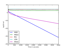
(a) on DIR dataset

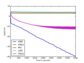
(b) on CTM dataset

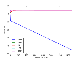
(c) on NEG dataset

Figure 1: The performance of different algorithms on the three datasets. The $x$-axis is the running time (in seconds), the $y$-axis is the logarithm of the total correlation error.

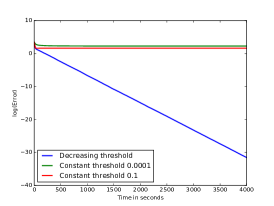
(a) different thresholds on DIR

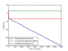
(b) different thresholds on CTM

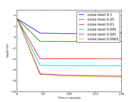
(c) robustness to noise

Figure 2: The performance of the algorithm AND with different thresholding schemes, and its robustness to noise. The $x$-axis is the running time (in seconds), the $y$-axis is the logarithm of the total correlation error. (a)(b) Using different thresholding schemes on the DIR/CTM dataset. “Decreasing thresold” refers to the scheme used in the original AND, “Constant threshold $c$” refers to using the threshold value $c$ throughout all iterations. (c) The performance in the presence of noises of various levels.

Evaluation criterion.

Given the output matrix $\mathbb{A}$ and the ground truth matrix $\mathbb{A}^{*}$, the correlation error of the $i$-th column is given by

$$\varepsilon_{i}(\mathbb{A},\mathbb{A}^{*})=\min_{j\in[D],\sigma\in\mathbb{R}}\{\|[\mathbb{A}^{*}]^{i}-\sigma[\mathbb{A}]^{j}\|_{2}\}.$$

Thus, the error measures how well the $i$-th column of $\mathbb{A}^{*}$ is covered by the best column of $\mathbb{A}$ up to scaling. We find the best column since in some competitor algorithms, the columns of the solution $\mathbb{A}$ may only correspond to a permutation of the columns of $\mathbb{A}^{*}$.

We also define the total correlation error as

$$\varepsilon(\mathbb{A},\mathbb{A}^{*})=\sum_{i=1}^{D}\varepsilon_{i}(\mathbb{A},\mathbb{A}^{*}).$$

We report the total correlation error in all the experiments.

Initialization.

In all the experiments, the initialization matrix $\mathbb{A}_{0}$ is set to $\mathbb{A}_{0}=\mathbb{A}^{*}(\mathbb{I}+\mathbb{U})$ where $\mathbb{I}$ is the identity matrix and $\mathbb{U}$ is a matrix whose entries are i.i.d. samples from the uniform distribution on $[-0.05,0.05)$. Note that this is a very weak initialization, since $[\mathbb{A}_{0}]^{i}=(1+\mathbb{U}_{i,i})[\mathbb{A}^{*}]^{i}+\sum_{j\neq i}\mathbb{U}_{j,i}[\mathbb{A}^{*}]^{j}$ and the magnitude of the noise component $\sum_{j\neq i}\mathbb{U}_{j,i}[\mathbb{A}^{*}]^{j}$ can be larger than the signal part $(1+\mathbb{U}_{i,i})[\mathbb{A}^{*}]^{i}$.

Hyperparameters and Implementations.

For most experiments of AND, we used $T=50$ iterations for each stage, and thresholds $\alpha_{i}=0.1/(1.1)^{i-1}$. For experiments on the robustness to noise, we found $T=100$ leads to better performance. Furthermore, for all the experiments, instead of using one data point at each step, we used the whole dataset for update.

7.1 Convergence to the Ground-Truth

Figure 1 shows the convergence rate of the algorithms on the three datasets. AND converges in linear rate on all three datasets (note that the $y$-axis is in log-scale). HALS converges on the DIR and CTM datasets, but the convergence is in slower rates. Also, on CTM, the error oscillates. Furthermore, it doesn’t converge on NEG where the ground-truth matrix has negative entries. ANLS converges on DIR and CTM at a very slow speed due to the non-negative least square computation in each iteration. All the other algorithms do not converge to the ground-truth, suggesting that they do not have recovery guarantees.

7.2 The Threshold Schemes

Figure 2(a) shows the results of using different thresholding schemes on DIR, while Figure 2(b) shows that those on CTM. When using a constant threshold for all iterations, the error only decreases for the first few steps and then stop decreasing. This aligns with our analysis and is in strong contrast to the case with decreasing thresholds.

7.3 Robustness to Noise

Figure 2(c) shows the performance of AND on the NOISE dataset with various noise levels $\gamma$. The error drops at the first few steps, but then stabilizes around a constant related to the noise level, as predicted by our analysis. This shows that it can recover the ground-truth to good accuracy, even when the data have a significant amount of noise.

Appendix A Complete Proofs

We now recall the proof sketch.

For simplicity, we only focus on one stage and the expected update. The expected update of $\mathbb{A}^{(t)}$ is given by

$$\mathbb{A}^{(t+1)}=\mathbb{A}^{(t)}+\eta(\mathbb{E}[yz^{\top}]-\mathbb{A}^{(t)}\mathbb{E}[zz^{\top}]).$$

Let us write $\mathbb{A}=\mathbb{A}^{*}(\mathbb{\Sigma}_{0}+\mathbb{E}_{0})$ where $\mathbb{\Sigma}_{0}$ is diagonal and $\mathbb{E}_{0}$ is off-diagonal. Then the decoding is given by

$$z=\phi_{\alpha}(\mathbb{A}^{\dagger}x)=\phi_{\alpha}((\mathbb{\Sigma}_{0}+\mathbb{E}_{0})^{-1}x).$$

Let $\mathbb{\Sigma},\mathbb{E}$ be the diagonal part and the off-diagonal part of $(\mathbb{\Sigma}_{0}+\mathbb{E}_{0})^{-1}$.

The first step of our analysis is a key lemma for decoding. It says that under suitable conditions, $z$ will be close to $\mathbb{\Sigma}x$ in the following sense:

$$\mathbb{E}[\mathbb{\Sigma}xx^{\top}]\approx\mathbb{E}[zx^{\top}],~{}~{}\mathbb{E}[\mathbb{\Sigma}xz^{\top}]\approx\mathbb{E}[zz^{\top}].$$

This key decoding lemma is formally stated in Lemma 6 (for the simplified case where $x\in\{0,1\}^{D}$) and Lemma 8 (for the general case where $x\in[0,1]^{D}$).

Now, let us write $\mathbb{A}^{(t)}=\mathbb{A}^{*}(\mathbb{\Sigma}_{t}+\mathbb{E}_{t})$. Then applying the above decoding lemma, the expected update of $\mathbb{\Sigma}_{t}+\mathbb{E}_{t}$ is

$$\mathbb{\Sigma}_{t+1}+\mathbb{E}_{t+1}=(\mathbb{\Sigma}_{t}+\mathbb{E}_{t})(\mathbb{I}-\mathbb{\Sigma}\mathbb{\Delta}\mathbb{\Sigma})+\mathbb{\Sigma}^{-1}(\mathbb{\Sigma}\mathbb{\Delta}\mathbb{\Sigma})+\mathbb{R}_{t}$$

where $\mathbb{R}_{t}$ is a small error term.

The second step is a key lemma for updating the feature matrix: for the update rule

$$\mathbb{\Sigma}_{t+1}+\mathbb{E}_{t+1}=(\mathbb{\Sigma}_{t}+\mathbb{E}_{t})(1-\eta\mathbb{\Lambda})+\eta\mathbb{Q}\mathbb{\Lambda}+\eta\mathbb{R}_{t}$$

where $\mathbb{\Lambda}$ is a PSD matrix and $\|\mathbb{R}_{t}\|_{2}\leq C^{\prime\prime}$, we have

$$\|\mathbb{\Sigma}_{t}+\mathbb{E}_{t}-\mathbb{Q}\|_{2} \leq\|\mathbb{\Sigma}_{0}+\mathbb{E}_{0}-\mathbb{Q}\|_{2}(1-\eta\lambda_{\min}(\mathbb{\Lambda}))^{t}+\frac{C^{\prime\prime}}{\lambda_{\min}(\mathbb{\Lambda})}.$$

This key updating lemma is formally stated in Lemma 10.

Applying this on our update rule with $\mathbb{Q}=\mathbb{\Sigma}^{-1}$ and $\mathbb{\Lambda}=\mathbb{\Sigma}\mathbb{\Delta}\mathbb{\Sigma}$, we know that when the error term is sufficiently small, we can make progress on $\|\mathbb{\Sigma}_{t}+\mathbb{E}_{t}-\mathbb{\Sigma}^{-1}\|_{2}$. Then, by using the fact that $\mathbb{\Sigma}_{0}\approx\mathbb{I}$ and $\mathbb{E}_{0}$ is small, and the fact that $\mathbb{\Sigma}$ is the diagonal part of $(\mathbb{\Sigma}_{0}+\mathbb{E}_{0})^{-1}$, we can show that after sufficiently many iterations, $\|\mathbb{\Sigma}_{t}-\mathbb{I}\|_{2}$ blows up slightly, while $\|\mathbb{E}_{t}\|_{2}$ is reduced significantly (See Lemma 11 for the formal statement). Repeating this for multiple stages completes the proof.

Organization.

Following the proof sketch, we first present the decoding lemmas in Section A.1, and then the update lemmas in Section A.2. Section A.3 then uses these lemmas to prove the main theorems (Theorem 1 and Theorem 4). Proving the decoding lemmas is highly non-trivial, and we collect the lemmas needed in Section A.4.

Finally, the analysis for the robustness to noise follows a similar proof sketch. It is presented in Section A.5.

A.1 Decoding

A.1.1 $x_{i}\in\{0,1\}$

Here we present the following decoding Lemma when $x_{i}\in\{0,1\}$.

Lemma 6 (Decoding).

For every $\ell\in[0,1)$, every off-diagonal matrix $\mathbb{E}^{\prime}$ such that $\|\mathbb{E}^{\prime}\|_{2}\leq\ell$ and every diagonal matrix $\mathbb{\Sigma}^{\prime}$ such that $\|\mathbb{\Sigma}^{\prime}-\mathbb{I}\|_{2}\leq\frac{1}{2}$, let $z=\phi_{\alpha}((\mathbb{\Sigma}^{\prime}+\mathbb{E}^{\prime})x)$ for $\alpha\leq\frac{1}{4}$. Then for every $\beta\in(0,1/2]$,

$$\|\mathbb{E}[(\mathbb{\Sigma}^{\prime}x-z)x^{\top}]\|_{2},\|\mathbb{E}[(\mathbb{\Sigma}^{\prime}x-z)z^{\top}]\|_{2}=O(C_{1})$$

where

$$C_{1}=\frac{kr}{D}+\frac{m\ell^{4}r^{2}}{\alpha^{3}D^{2}}+\frac{\ell^{2}\sqrt{km}r^{1.5}}{D^{1.5}\beta}+\frac{\ell^{4}r^{3}m}{\beta^{2}D^{2}}+\frac{\ell^{5}r^{2.5}m}{D^{2}\alpha^{2}\beta}.$$

Proof of Lemma 6.

We will prove the bound on $\|\mathbb{E}[(\mathbb{\Sigma}^{\prime}x-z)z^{\top}]\|_{2}$, and a simlar argument holds for that on $\|\mathbb{E}[(\mathbb{\Sigma}^{\prime}x-z)x^{\top}]\|_{2}$.

First consider the term $|\mathbb{\Sigma}_{i,i}^{\prime}x_{i}-z_{i}|$ for a fixed $i\in[D]$. Due to the decoding, we have $z_{i}=\phi_{\alpha}([(\mathbb{\Sigma}^{\prime}+\mathbb{E}^{\prime})]_{i}x)=\phi_{\alpha}(\mathbb{\Sigma}_{i,i}^{\prime}x_{i}+\langle e_{i},x\rangle)$ where $e_{i}$ is the $i$-th row of $\mathbb{E}^{\prime}$.

Claim 7.

$$\mathbb{\Sigma}_{i,i}^{\prime}x_{i}-z_{i}=a_{x,1}\phi_{\alpha}(-\langle e_{i},x\rangle)+a_{x,2}\phi_{\alpha}(\langle e_{i},x\rangle)-\langle e_{i},x\rangle x_{i}$$ (A.1)

where $a_{x,1},a_{x,2}\in[-1,1]$ that depends on $x$.

Proof.

To see this, we split into two cases:

1. When $x_{i}=0$, then $|\mathbb{\Sigma}_{i,i}^{\prime}x_{i}-z_{i}|=|z_{i}|\leq\phi_{\alpha}(\langle e_{i},x\rangle)$.

2. When $x_{i}=1$, then $z_{i}=0$ only when $-\langle e_{i},x\rangle\geq\frac{1}{2}-\alpha\geq\alpha$, which implies that $|\mathbb{\Sigma}_{i,i}^{\prime}x_{i}-z_{i}+\langle e_{i},x\rangle|\leq\alpha\leq\phi_{\alpha}(-\langle e_{i},x\rangle)$. When $\mathbb{\Sigma}_{i,i}^{\prime}x_{i}-z_{i}+\langle e_{i},x\rangle\not=0$, then $\mathbb{\Sigma}_{i,i}^{\prime}x_{i}-z_{i}=-\langle e_{i},x\rangle$.

Putting everything together, we always have:

$$|\mathbb{\Sigma}_{i,i}^{\prime}x_{i}-z_{i}+\langle{e}_{i},x\rangle x_{i}|\leq\phi_{\alpha}(|\langle e_{i},x\rangle|)$$

which means that there exists $a_{x,1},a_{x,2}\in[-1,1]$ that depend on $x$ such that

$$\mathbb{\Sigma}_{i,i}^{\prime}x_{i}-z_{i}=a_{x,1}\phi_{\alpha}(-\langle e_{i},x\rangle)+a_{x,2}\phi_{\alpha}(\langle e_{i},x\rangle)-\langle e_{i},x\rangle x_{i}.$$

∎

Consider the term $\langle e_{i},x\rangle x_{i}$, we know that for every $\beta\geq 0$,

$$|\langle e_{i},x\rangle-\phi_{\beta}(\langle e_{i},x\rangle)+\phi_{\beta}(-\langle e_{i},x\rangle)|\leq\beta.$$

Therefore, there exists $b_{x}\in[-\beta,\beta]$ that depends on $x$ such that

$$\langle e_{i},x\rangle x_{i}=\phi_{\beta}(\langle e_{i},x\rangle)-\phi_{\beta}(-\langle e_{i},x\rangle)-b_{x}x_{i}.$$

Putting into (A.1), we get:

$$\mathbb{\Sigma}_{i,i}^{\prime}x_{i}-z_{i}=a_{x,1}\phi_{\alpha}(-\langle e_{i},x\rangle)+a_{x,2}\phi_{\alpha}(\langle e_{i},x\rangle)-\phi_{\beta}(\langle{e}_{i},x\rangle)x_{i}+\phi_{\beta}(-\langle{e}_{i},x\rangle)x_{i}+b_{x}x_{i}.$$

For notation simplicity, let us now write

$$z_{i}=(\mathbb{\Sigma}_{i,i}^{\prime}-b_{x})x_{i}+a_{i}+b_{i}$$

where

$$a_{i}=-a_{x,1}\phi_{\alpha}(-\langle e_{i},x\rangle)-a_{x,2}\phi_{\alpha}(\langle e_{i},x\rangle),\quad b_{i}=\phi_{\beta}(\langle{e}_{i},x\rangle)x_{i}-\phi_{\beta}(-\langle{e}_{i},x\rangle)x_{i}.$$

We then have

$$(\mathbb{\Sigma}_{i,i}^{\prime}x_{i}-z_{i})z_{j}=(b_{x}x_{i}-a_{i}-b_{i})((\mathbb{\Sigma}_{j,j}^{\prime}-b_{x})x_{j}+a_{j}+b_{j}).$$

Let us now construct matrix $\mathbb{M}_{1},\cdots\mathbb{M}_{9}$, whose entries are given by

1. $(\mathbb{M}_{1})_{i,j}=b_{x}x_{i}(\mathbb{\Sigma}_{j,j}^{\prime}-b_{x})x_{j}$

2. $(\mathbb{M}_{2})_{i,j}=b_{x}x_{i}a_{j}$

3. $(\mathbb{M}_{3})_{i,j}=b_{x}x_{i}b_{j}$

4. $(\mathbb{M}_{4})_{i,j}=-a_{i}(\mathbb{\Sigma}_{j,j}^{\prime}-b_{x})x_{j}$

5. $(\mathbb{M}_{5})_{i,j}=-a_{i}a_{j}$

6. $(\mathbb{M}_{6})_{i,j}=-a_{i}b_{j}$

7. $(\mathbb{M}_{7})_{i,j}=-b_{i}(\mathbb{\Sigma}_{j,j}^{\prime}-b_{x})x_{j}$

8. $(\mathbb{M}_{8})_{i,j}=-b_{i}a_{j}$

9. $(\mathbb{M}_{9})_{i,j}=-b_{i}b_{j}$

Thus, we know that $\mathbb{E}[(\mathbb{\Sigma}^{\prime}x-z)z^{\top}]=\sum_{i=1}^{9}\mathbb{E}[\mathbb{M}_{i}]$. It is sufficient to bound the spectral norm of each matrices separately, as we discuss below.

1. $\mathbb{M}_{2},\mathbb{M}_{4}$: these matrices can be bounded by Lemma 14, term 1.

2. $\mathbb{M}_{5}$: this matrix can be bounded by Lemma 14, term 2.

3. $\mathbb{M}_{6},\mathbb{M}_{8}$: these matrices can be bounded by Lemma 15, term 3.

4. $\mathbb{M}_{3},\mathbb{M}_{7}$: these matrices can be bounded by Lemma 15, term 2.

5. $\mathbb{M}_{9}$: this matrix can be bounded by Lemma 15, term 1.

6. $\mathbb{E}[\mathbb{M}_{1}]$: this matrix is of the form $\mathbb{E}[b_{x}x(x\odot d_{x})^{\top}]$, where $d_{x}$ is a vector whose $j$-th entry is $(\mathbb{\Sigma}_{j,j}^{\prime}-b_{x})$.

   To bound the this term, we have that for any $u,v$ such that $\|u\|_{2}=\|v\|_{2}=1$,

   $$u^{\top}\mathbb{E}[b_{x}x(x\odot d_{x})^{\top}]v = \mathbb{E}[b_{x}\langle u,x\rangle\langle v,x\odot d_{x}\rangle].$$

   When $\beta\leq\frac{1}{2}$, since $x$ is non-negative, we know that the maximum of $\mathbb{E}[b_{x}\langle u,x\rangle\langle v,x\odot d_{x}\rangle]$ is obtained when $b_{x}=\beta$, $d_{x}=(2,\cdots,2)$ and $u,v$ are all non-negative, which gives us

   $$\mathbb{E}[b_{x}\langle u,x\rangle\langle v,x\odot d_{x}\rangle]\leq 2\beta\|\mathbb{E}[xx^{\top}]\|_{2}\leq\sqrt{\|\mathbb{E}[xx^{\top}]\|_{1}\|\mathbb{E}[xx^{\top}]\|_{\infty}}=\|\mathbb{E}[xx^{\top}]\|_{1}.$$

   Now, for each row of $\|\mathbb{E}[xx^{\top}]\|_{1}$, we know that $[\mathbb{E}[xx^{\top}]]_{i}\leq\mathbb{E}[x_{i}\sum_{j}x_{j}]\leq\frac{2rk}{D}$, which gives us

   $$\|\mathbb{E}[\mathbb{M}_{1}]\|_{2}\leq\frac{4\beta rk}{D}.$$

Putting everything together gives the bound on $\|\mathbb{E}[(\mathbb{\Sigma}^{\prime}x-z)z^{\top}]\|_{2}$. A similar proof holds for the bound on $\|\mathbb{E}[(\mathbb{\Sigma}^{\prime}x-z)x^{\top}]\|_{2}$. ∎

A.1.2 General $x_{i}$

We have the following decoding lemma for the general case when $x_{i}\in[0,1]$ and the distribution of $x$ satisfies the order-$q$ decay condition.

Lemma 8 (Decoding II).

For every $\ell\in[0,1)$, every off-diagonal matrix $\mathbb{E}^{\prime}$ such that $\|\mathbb{E}^{\prime}\|_{2}\leq\ell$ and every diagonal matrix $\mathbb{\Sigma}^{\prime}$ such that $\|\mathbb{\Sigma}^{\prime}-\mathbb{I}\|_{2}\leq\frac{1}{2}$, let $z=\phi_{\alpha}((\mathbb{\Sigma}^{\prime}+\mathbb{E}^{\prime})x)$ for $\alpha\leq\frac{1}{4}$. Then for every $\beta\in(0,\alpha]$,

$$\|\mathbb{E}[(\mathbb{\Sigma}^{\prime}x-z)x^{\top}]\|_{2},\|\mathbb{E}[(\mathbb{\Sigma}^{\prime}x-z)z^{\top}]\|_{2}=O(C_{2})$$

where

$$C_{2}=\frac{\ell^{4}r^{3}m}{\alpha\beta^{2}D^{2}}+\frac{\ell^{5}r^{2.5}m}{D^{2}\alpha^{2.5}\beta}+\frac{\ell^{2}kr}{D\beta}\left(\frac{m}{Dk}\right)^{\frac{q}{2q+2}}+\frac{\ell^{3}r^{2}\sqrt{km}}{D^{1.5}\alpha^{2}}+\frac{\ell^{6}r^{4}m}{\alpha^{4}D^{2}}+k\beta\left(\frac{r}{D}\right)^{\frac{2q+1}{2q+2}}+\frac{kr}{D}\alpha^{\frac{q+1}{2}}.$$

Proof of Lemma 8.

We consider the bound on $\|\mathbb{E}[(\mathbb{\Sigma}^{\prime}x-z)z^{\top}]\|_{2}$, and that on $\mathbb{E}[(\mathbb{\Sigma}^{\prime}x-z)x^{\top}]\|_{2}$ can be proved by a similar argument.

Again, we still have

$$z_{i}=\phi_{\alpha}([(\mathbb{\Sigma}^{\prime}+\mathbb{E}^{\prime})]_{i}x)=\phi_{\alpha}(\mathbb{\Sigma}_{i,i}^{\prime}x_{i}+\langle e_{i},x\rangle).$$

However, this time even when $x_{i}\not=0$, $x_{i}$ can be smaller than $\alpha$. Therefore, we need the following inequality.

Claim 9.

$$|\mathbb{\Sigma}_{i,i}^{\prime}x_{i}-z_{i}+\langle{e}_{i},x\rangle\mathsf{1}_{x_{i}\geq 4\alpha}|\leq\phi_{\alpha/2}(|\langle e_{i},x\rangle|)+2x_{i}\mathsf{1}_{x_{i}\in(0,4\alpha)}.$$

Proof.

To see this, we can consider the following four events:

1. $x_{i}=0$, then $|\mathbb{\Sigma}_{i,i}^{\prime}x_{i}-z_{i}+\langle{e}_{i},x\rangle\mathsf{1}_{x_{i}\geq 2\alpha}|=|z_{i}|\leq\phi_{\alpha}(\langle e_{i},x\rangle)$

2. $x_{i}\geq 4\alpha$. $|\mathbb{\Sigma}_{i,i}^{\prime}x_{i}-z_{i}+\langle{e}_{i},x\rangle\mathsf{1}_{x_{i}\geq 4\alpha}|=|\mathbb{\Sigma}_{i,i}^{\prime}x_{i}+\langle e_{i},x\rangle-\phi_{\alpha}(\mathbb{\Sigma}_{i,i}^{\prime}x_{i}+\langle e_{i},x\rangle)|$. Since $\mathbb{\Sigma}_{i,i}^{\prime}x_{i}\geq 2\alpha$, we can get the same bound.

3. $x_{i}\in(\alpha/4,4\alpha)$: then if $z_{i}\not=0$, $|\mathbb{\Sigma}_{i,i}^{\prime}x_{i}-z_{i}+\langle e_{i},x\rangle|=0$. Which implies that

   $$|\mathbb{\Sigma}_{i,i}^{\prime}x_{i}-z_{i}|\leq|\langle e_{i},x\rangle|\leq\phi_{\alpha/2}(|\langle e_{i},x\rangle|)+\frac{\alpha}{2}\leq\phi_{\alpha/2}(|\langle e_{i},x\rangle|)+2x_{i}\mathsf{1}_{x_{i}\in(0,4\alpha)}$$

   If $z_{i}=0$, then

   $$|\mathbb{\Sigma}_{i,i}^{\prime}x_{i}-z_{i}|=\mathbb{\Sigma}_{i,i}^{\prime}x_{i}\leq 2x_{i}\mathsf{1}_{x_{i}\in(0,2\alpha)}$$

4. $x_{i}\in(0,\alpha/4)$, then $\mathbb{\Sigma}_{i,i}^{\prime}x_{i}\leq\frac{\alpha}{2}$, therefore, $z_{i}\not=0$ only when $\langle e_{i},x\rangle\geq\frac{\alpha}{2}$. We still have: $|\mathbb{\Sigma}_{i,i}^{\prime}x_{i}-z_{i}|\leq\phi_{\alpha/2}(\langle e_{i},x\rangle)$

   If $z_{0}=0$, then $|\mathbb{\Sigma}_{i,i}^{\prime}x_{i}-z_{i}|\leq 2x_{i}\mathsf{1}_{x_{i}\in(0,4\alpha)}$ as before.

Putting everything together, we have the claim. ∎

Following the exact same calculation as in Lemma 6, we can obtain

$$\mathbb{\Sigma}_{i,i}^{\prime}x_{i}-z_{i} =a_{x,1}\phi_{\alpha/2}(-\langle e_{i},x\rangle)+a_{x,2}\phi_{\alpha/2}(\langle e_{i},x\rangle)$$

$$-\phi_{\beta}(\langle{e}_{i},x\rangle)\mathsf{1}_{x_{i}\geq 4\alpha}+\phi_{\beta}(-\langle{e}_{i},x\rangle)\mathsf{1}_{x_{i}\geq 4\alpha}$$

$$+b_{x}\mathsf{1}_{x_{i}\geq 4\alpha}+c_{x}2x_{i}\mathsf{1}_{x_{i}\in(0,4\alpha)}$$

for $a_{x,1},a_{x,1},c_{x}\in[-1,1]$ and $b_{x}\in[-\beta,\beta]$.

Therefore, consider a matrix $\mathbb{M}$ whose $(i,j)$-th entry is $(\mathbb{\Sigma}_{i,i}^{\prime}x_{i}-z_{i})z_{j}$. This entry can be written as the summation of the following terms.

1. Terms that can be bounded by Lemma 14. These include

   $$a_{x,1}\phi_{\alpha/2}(-\langle e_{i},x\rangle)x_{j},\quad a_{x,2}\phi_{\alpha/2}(\langle e_{i},x\rangle)x_{j},\quad a_{x,u}a_{x,v}\phi_{\alpha/2}((-1)^{u}\langle e_{i},x\rangle)\phi_{\alpha/2}((-1)^{v}\langle e_{j},x\rangle)$$

   for $u,v\in\{1,2\}$, and

   $$a_{x,u}b_{x}\phi_{\alpha/2}((-1)^{u}\langle e_{i},x\rangle)\mathsf{1}_{x_{i}\geq 4\alpha},\quad 2a_{x,u}c_{x}\phi_{\alpha/2}((-1)^{u}\langle e_{i},x\rangle)x_{j}\mathsf{1}_{x_{j}\in(0,4\alpha)}$$

   by using $0\leq\mathsf{1}_{x_{j}\geq 4\alpha}\leq\frac{x_{j}}{4\alpha}$ and $0\leq x_{j}\mathsf{1}_{x_{j}\in(0,4\alpha)}\leq x_{j}$.

2. Terms that can be bounded by Lemma 21. These include

   $$-\phi_{\beta}(\langle{e}_{i},x\rangle)\mathsf{1}_{x_{i}\geq 4\alpha}x_{j},\quad\phi_{\beta}(-\langle{e}_{i},x\rangle)\mathsf{1}_{x_{i}\geq 4\alpha}x_{j},$$

   $$(-1)^{u}a_{x,v}\phi_{\beta}((-1)^{1+u}\langle{e}_{i},x\rangle)\mathsf{1}_{x_{i}\geq 4\alpha}\phi_{\alpha/2}((-1)^{v}\langle e_{j},x\rangle),$$

   $$(-1)^{u+v}\phi_{\beta}((-1)^{1+u}\langle{e}_{i},x\rangle)\mathsf{1}_{x_{i}\geq 4\alpha}\mathsf{1}_{x_{j}\geq 4\alpha}\phi_{\beta}((-1)^{1+v}\langle{e}_{j},x\rangle)$$

   for $u,v\in\{1,2\}$. Also include

   $$2(-1)^{u}c_{x}\phi_{\beta}((-1)^{1+u}\langle{e}_{i},x\rangle)\mathsf{1}_{x_{i}\geq 4\alpha}x_{j}\mathsf{1}_{x_{j}\in(0,4\alpha)}$$

   by using$0\leq x_{j}\mathsf{1}_{x_{j}\in(0,4\alpha)}\leq x_{j}$. Also include

   $$2(-1)^{u}b_{x}\phi_{\beta}((-1)^{1+u}\langle{e}_{i},x\rangle)\mathsf{1}_{x_{i}\geq 4\alpha}\mathsf{1}_{x_{j}\geq 4\alpha}$$

   by using $0\leq\mathsf{1}_{x_{j}\geq 4\alpha}\leq\frac{x_{j}}{4\alpha}$.

3. Terms that can be bounded by Lemma 18. These include

   $$b_{x}\mathsf{1}_{x_{i}\geq 4\alpha}x_{j},\quad b_{x}^{2}\mathsf{1}_{x_{i}\geq 4\alpha}\mathsf{1}_{x_{j}\geq 4\alpha},\quad 2b_{x}c_{x}\mathsf{1}_{x_{i}\geq 4\alpha}x_{i}\mathsf{1}_{x_{j}\in(0,4\alpha)}x_{j}.$$

   Where agin we use the fact that $0\leq\mathsf{1}_{x_{i}\geq 4\alpha}\leq\frac{x_{j}}{4\alpha}$ and $0\leq x_{i},\mathsf{1}_{x_{j}\in(0,4\alpha)}\leq 1$

4. Terms that can be bounded by Lemma 17. These include

   $$c_{x}2x_{i}\mathsf{1}_{x_{i}\in(0,4\alpha)}x_{j},\quad 4c_{x}^{2}x_{i}\mathsf{1}_{x_{i}\in(0,4\alpha)}x_{j}\mathsf{1}_{x_{j}\in(0,4\alpha)}.$$

   Where we use the fact that $0\leq\mathsf{1}_{x_{j}\in(0,4\alpha)}\leq 1$.

Putting everything together, when $0<\beta\leq\alpha$,

$$\|\mathbb{E}[(\mathbb{\Sigma}^{\prime}x-z)z^{\top}]\|_{2}=O\left(C_{2}\right)$$

where

$$C_{2}=\frac{\ell^{4}r^{3}m}{\alpha\beta^{2}D^{2}}+\frac{\ell^{5}r^{2.5}m}{D^{2}\alpha^{2.5}\beta}+\frac{\ell^{2}kr}{D\beta}\left(\frac{m}{Dk}\right)^{\frac{q}{2q+2}}+\frac{\ell^{3}r^{2}\sqrt{km}}{D^{1.5}\alpha^{2}}+\frac{\ell^{6}r^{4}m}{\alpha^{4}D^{2}}+k\beta\left(\frac{r}{D}\right)^{\frac{2q+1}{2q+2}}+\frac{kr}{D}\alpha^{\frac{q+1}{2}}.$$

This gives the bound on $\mathbb{E}[(\mathbb{\Sigma}^{\prime}x-z)z^{\top}]\|_{2}$. The bound on $\mathbb{E}[(\mathbb{\Sigma}^{\prime}x-z)x^{\top}]\|_{2}$ can be proved by a similar argument.

∎

A.2 Update

A.2.1 General Update Lemma

Lemma 10 (Update).

Suppose $\mathbb{\Sigma}_{t}$ is diagonal and $\mathbb{E}_{t}$ is off-diagonal for all $t$. Suppose we have an update rule that is given by

$$\mathbb{\Sigma}_{t+1}+\mathbb{E}_{t+1}=(\mathbb{\Sigma}_{t}+\mathbb{E}_{t})(1-\eta\mathbb{\Delta})+\eta\mathbb{\Sigma}\mathbb{\Delta}+\eta\mathbb{R}_{t}$$

for some positive semidefinite matrix $\mathbb{\Delta}$ and some $\mathbb{R}_{t}$ such that $\|\mathbb{R}_{t}\|_{2}\leq C^{\prime\prime}$. Then for every $t\geq 0$,

$$\|\mathbb{\Sigma}_{t}+\mathbb{E}_{t}-\mathbb{\Sigma}\|_{2}\leq\|\mathbb{\Sigma}_{0}+\mathbb{E}_{0}-\mathbb{\Sigma}\|_{2}(1-\eta\lambda_{\min}(\mathbb{\Delta}))^{t}+\frac{C^{\prime\prime}}{\lambda_{\min}(\mathbb{\Delta})}.$$

Proof of Lemma 10.

We know that the update is given by

$$\mathbb{\Sigma}_{t+1}+\mathbb{E}_{t+1}-\mathbb{\Sigma}=(\mathbb{\Sigma}_{t}+\mathbb{E}_{t}-\mathbb{\Sigma})(1-\eta\mathbb{\Delta})+\eta\mathbb{R}_{t}.$$

If we let

$$\mathbb{\Sigma}_{t}+\mathbb{E}_{t}-\mathbb{\Sigma}=(\mathbb{\Sigma}_{0}+\mathbb{E}_{0}-\mathbb{\Sigma})(1-\eta\mathbb{\Delta})^{t}+\mathbb{C}_{t}.$$

Then we can see that the update rule of $\mathbb{C}_{t}$ is given by

$$\mathbb{C}_{0} =0,$$

$$\mathbb{C}_{t+1} =\mathbb{C}_{t}(1-\eta\mathbb{\Delta})+\eta\mathbb{R}_{t}$$

which implies that $\forall t\geq 0,\|\mathbb{C}_{t}\|_{2}\leq\frac{C^{\prime\prime}}{\lambda_{\min}(\mathbb{\Delta})}$.

Putting everything together completes the proof. ∎

Lemma 11 (Stage).

In the same setting as Lemma 10, suppose initially for $\ell_{1},\ell_{2}\in[0,\frac{1}{8})$ we have

$$\|\mathbb{\Sigma}_{0}-\mathbb{I}\|_{2}\leq\ell_{1},\|\mathbb{E}_{0}\|\leq\ell_{2},\mathbb{\Sigma}=(\textsf{Diag}[(\mathbb{\Sigma}_{0}+\mathbb{E}_{0})^{-1}])^{-1}.$$

Moreover, suppose in each iteration, the error $\mathbb{R}_{t}$ satisfies that $\|\mathbb{R}_{t}\|_{2}\leq\frac{\lambda_{\min}(\mathbb{\Delta})}{160}\ell_{2}$.

Then after $t=\frac{\log\frac{400}{\ell_{2}}}{\eta\lambda_{\min}(\mathbb{\Delta})}$ iterations, we have

1. $\|\mathbb{\Sigma}_{t}-\mathbb{I}\|_{2}\leq\ell_{1}+4\ell_{2}$,

2. $\|\mathbb{E}_{t}\|_{2}\leq\frac{1}{40}\ell_{2}$.

Proof of Lemma 11.

Using Taylor expansion, we know that

$$\textsf{Diag}[(\mathbb{\Sigma}_{0}+\mathbb{E}_{0})^{-1}]=\mathbb{\Sigma}_{0}^{-1}+\sum_{i=1}^{\infty}\mathbb{\Sigma}_{0}^{-1/2}\textsf{Diag}[(-\mathbb{\Sigma}_{0}^{-1/2}\mathbb{E}_{0}\mathbb{\Sigma}_{0}^{-1/2})^{i}]\mathbb{\Sigma}_{0}^{-1/2}.$$

Since $\|\textsf{Diag}(\mathbb{M})\|_{2}\leq\|\mathbb{M}\|_{2}$ for any matrix $\mathbb{M}$,

$$\|\textsf{Diag}[(\mathbb{\Sigma}_{0}+\mathbb{E}_{0})^{-1}]-\mathbb{\Sigma}_{0}^{-1}\|_{2} =\|\sum_{i=1}^{\infty}\mathbb{\Sigma}_{0}^{-1/2}\textsf{Diag}[(-\mathbb{\Sigma}_{0}^{-1/2}\mathbb{E}_{0}\mathbb{\Sigma}_{0}^{-1/2})^{i}]\mathbb{\Sigma}_{0}^{-1/2}\|_{2}$$

$$\leq\|\sum_{i=1}^{\infty}\mathbb{\Sigma}_{0}^{-1/2}(-\mathbb{\Sigma}_{0}^{-1/2}\mathbb{E}_{0}\mathbb{\Sigma}_{0}^{-1/2})^{i}\mathbb{\Sigma}_{0}^{-1/2}\|_{2}$$

$$=\|[(\mathbb{\Sigma}_{0}+\mathbb{E}_{0})^{-1}](-\mathbb{E}_{0}\mathbb{\Sigma}_{0}^{-1})\|_{2}$$

$$\leq\frac{\ell_{2}}{(1-\ell_{1})(1-\ell_{1}-\ell_{2})}\leq\frac{32}{21}\ell_{2}.$$

Therefore,

$$\|\textsf{Diag}[(\mathbb{\Sigma}_{0}+\mathbb{E}_{0})^{-1}]\mathbb{\Sigma}_{0}-\mathbb{I}\|_{2}\leq\frac{\ell_{2}(1+\ell_{1})}{(1-\ell_{1})(1-\ell_{1}-\ell_{2})}\leq\ell:=\frac{12}{7}\ell_{2}.$$

which gives us

$$\|\textsf{Diag}[(\mathbb{\Sigma}_{0}+\mathbb{E}_{0})^{-1}]^{-1}\mathbb{\Sigma}_{0}^{-1}-\mathbb{I}\|_{2}\leq\frac{\ell}{1-\ell}\leq\frac{24}{11}\ell_{2}.$$

This then leads to

$$\|\mathbb{\Sigma}-\mathbb{\Sigma}_{0}\|_{2}\leq\|\textsf{Diag}[(\mathbb{\Sigma}_{0}+\mathbb{E}_{0})^{-1}]^{-1}-\mathbb{\Sigma}_{0}\|_{2}\leq\frac{(1+\ell_{1})\ell}{1-\ell}\leq 3\ell_{2}.$$

Now since $\|\mathbb{\Sigma}_{0}+\mathbb{E}_{0}-\mathbb{\Sigma}\|_{2}\leq 4\ell_{2}\leq 1$, after $t=\frac{\log\frac{400}{\ell_{2}}}{\eta\lambda_{\min}(\mathbb{\Delta})}$ iterations, we have

$$\|\mathbb{\Sigma}_{t}+\mathbb{E}_{t}-\mathbb{\Sigma}\|_{2}\leq\frac{1}{80}\ell_{2}.$$

Then since $\mathbb{\Sigma}_{t}-\mathbb{\Sigma}=\textsf{Diag}[\mathbb{\Sigma}_{t}+\mathbb{E}_{t}-\mathbb{\Sigma}]$, we have

$$\|\mathbb{\Sigma}_{t}-\mathbb{\Sigma}\|_{2}\leq\|\mathbb{\Sigma}_{t}+\mathbb{E}_{t}-\mathbb{\Sigma}\|_{2}\leq\frac{1}{80}\ell_{2}.$$

This implies that

$$\|\mathbb{E}_{t}\|_{2}\leq\|\mathbb{\Sigma}_{t}-\mathbb{\Sigma}\|_{2}+\|\mathbb{\Sigma}_{t}+\mathbb{E}_{t}-\mathbb{\Sigma}\|_{2}\leq\frac{1}{40}\ell_{2}$$

and

$$\|\mathbb{\Sigma}_{t}-\mathbb{I}\|_{2}\leq\|\mathbb{\Sigma}_{t}-\mathbb{\Sigma}\|_{2}+\|\mathbb{\Sigma}-\mathbb{\Sigma}_{0}\|_{2}+\|\mathbb{\Sigma}_{0}-\mathbb{I}\|_{2}\leq\frac{1}{80}\ell_{2}+3\ell_{2}+\ell_{1}\leq\ell_{1}+4\ell_{2}.$$

∎

Corollary 12 (Corollary of Lemma 11).

Under the same setting as Lemma 11, suppose initially $\ell_{1}\leq\frac{1}{17}$, then

1. $\ell_{1}\leq\frac{1}{8}$ holds true through all stages,

2. $\ell_{2}\leq\left(\frac{1}{40}\right)^{t}$ after $t$ stages.

Proof of Corollary 12.

The second claim is trivial. For the first claim, we have

$$(\ell_{1})_{stage\ s+1}\leq(\ell_{1})_{stage\ s}+4(\ell_{2})_{stage\ s}\leq\cdots\leq\frac{1}{17}+\frac{1}{8}\sum_{i}(1/40)^{i}\leq\frac{1}{8}.$$

∎

A.3 Proof of the Main Theorems

With the update lemmas, we are ready to prove the main theorems.

Proof of Theorem 1.

For simplicity, we only focus on the expected update. The on-line version can be proved directly from this by noting that the variance of the update is polynomial bounded and setting accordingly a polynomially small $\eta$. The expected update of $\mathbb{A}^{(t)}$ is given by

$$\mathbb{A}^{(t+1)}=\mathbb{A}^{(t)}+\eta(\mathbb{E}[yz^{\top}]-\mathbb{A}^{(t)}\mathbb{E}[zz^{\top}])$$

Let us pick $\alpha=\frac{1}{4}$, focus on one stage and write $\mathbb{A}=\mathbb{A}^{*}(\mathbb{\Sigma}_{0}+\mathbb{E}_{0})$. Then the decoding is given by

$$z=\phi_{\alpha}(\mathbb{A}^{\dagger}x)=\phi_{\alpha}((\mathbb{\Sigma}_{0}+\mathbb{E}_{0})^{-1}x).$$

Let $\mathbb{\Sigma},\mathbb{E}$ be the diagonal part and the off diagonal part of $(\mathbb{\Sigma}_{0}+\mathbb{E}_{0})^{-1}$. By Lemma 6,

$$\|\mathbb{E}[(\mathbb{\Sigma}x-z)x^{\top}\mathbb{\Sigma}]\|_{2},\|\mathbb{E}[(\mathbb{\Sigma}x-z)z^{\top}\|_{2}=O(C_{1}).$$

Now, if we write $\mathbb{A}^{(t)}=\mathbb{A}^{*}(\mathbb{\Sigma}_{t}+\mathbb{E}_{t})$, then the expected update of $\mathbb{\Sigma}_{t}+\mathbb{E}_{t}$ is given by

$$\mathbb{\Sigma}_{t+1}+\mathbb{E}_{t+1}=(\mathbb{\Sigma}_{t}+\mathbb{E}_{t})(\mathbb{I}-\mathbb{\Sigma}\mathbb{\Delta}\mathbb{\Sigma})+\mathbb{\Sigma}^{-1}(\mathbb{\Sigma}\mathbb{\Delta}\mathbb{\Sigma})+\mathbb{R}_{t}$$

where $\|\mathbb{R}_{t}\|_{2}=O(C_{1})$.

By Lemma 11, as long as $C_{1}=O(\sigma_{\min}(\mathbb{\Delta})\|\mathbb{E}_{0}\|_{2})=O\left(\frac{k\lambda}{D}\|\mathbb{E}_{0}\|_{2}\right)$, we can make progress. Putting in the expression of $C_{1}$ with $\ell\geq\|\mathbb{E}_{0}\|_{2}$, we can see that as long as

$$\frac{\beta kr}{D}+\frac{m\ell^{4}r^{2}}{\alpha^{3}D^{2}}+\frac{\ell^{2}\sqrt{km}r^{1.5}}{D^{1.5}\beta}+\frac{\ell^{4}r^{3}m}{\beta^{2}D^{2}}+\frac{\ell^{5}r^{2.5}m}{D^{2}\alpha^{2}\beta}=O\left(\frac{k\lambda}{D}\ell\right),$$

we can make progress. By setting $\beta=O\left(\frac{\lambda\ell}{r}\right)$, with Corollary 12 we completes the proof. ∎

Proof of Theorem 4.

For simplicity, we only focus on the expected update. The on-line version can be proved directly from this by setting a polynomially small $\eta$. The expected update of $\mathbb{A}^{(t)}$ is given by

$$\mathbb{A}^{(t+1)}=\mathbb{A}^{(t)}+\eta(\mathbb{E}[yz^{\top}]-\mathbb{A}^{(t)}\mathbb{E}[zz^{\top}]).$$

Let us focus on one stage and write $\mathbb{A}=\mathbb{A}^{*}(\mathbb{\Sigma}_{0}+\mathbb{E}_{0})$. Then the decoding is given by

$$z=\phi_{\alpha}(\mathbb{A}^{\dagger}x)=\phi_{\alpha}((\mathbb{\Sigma}_{0}+\mathbb{E}_{0})^{-1}x).$$

Let $\mathbb{\Sigma},\mathbb{E}$ be the diagonal part and the off diagonal part of $(\mathbb{\Sigma}_{0}+\mathbb{E}_{0})^{-1}$. By Lemma 8,

$$\|\mathbb{E}[(\mathbb{\Sigma}x-z)x^{\top}\mathbb{\Sigma}]\|_{2},\|\mathbb{E}[(\mathbb{\Sigma}x-z)z^{\top}\|_{2}=O(C_{2}).$$

Now, if we write $\mathbb{A}^{(t)}=\mathbb{A}^{*}(\mathbb{\Sigma}_{t}+\mathbb{E}_{t})$, then the expected update of $\mathbb{\Sigma}_{t}+\mathbb{E}_{t}$ is given by

$$\mathbb{\Sigma}_{t+1}+\mathbb{E}_{t+1}=(\mathbb{\Sigma}_{t}+\mathbb{E}_{t})(\mathbb{I}-\mathbb{\Sigma}\mathbb{\Delta}\mathbb{\Sigma})+\mathbb{\Sigma}^{-1}(\mathbb{\Sigma}\mathbb{\Delta}\mathbb{\Sigma})+\mathbb{R}_{t}$$

where $\|\mathbb{R}_{t}\|_{2}=O(C_{2})$.

By Lemma 11, as long as $C_{2}=O(\sigma_{\min}(\mathbb{\Delta})\|\mathbb{E}_{0}\|_{2})=O\left(\frac{k\lambda}{D}\|\mathbb{E}_{0}\|_{2}\right)$, we can make progress. Putting in the expression of $C_{2}$ with $\ell\geq\|\mathbb{E}_{0}\|_{2}$, we can see that as long as

$$C_{2}=\frac{\ell^{4}r^{3}m}{\alpha\beta^{2}D^{2}}+\frac{\ell^{5}r^{2.5}m}{D^{2}\alpha^{2.5}\beta}+\frac{\ell^{2}kr}{D\beta}\left(\frac{m}{Dk}\right)^{\frac{q}{2q+2}}+\frac{\ell^{3}r^{2}\sqrt{km}}{D^{1.5}\alpha^{2}}+\frac{\ell^{6}r^{4}m}{\alpha^{4}D^{2}}+k\beta\left(\frac{r}{D}\right)^{\frac{2q+1}{2q+2}}+\frac{kr}{D}\alpha^{\frac{q+1}{2}}=O\left(\frac{k\lambda}{D}\ell\right),$$

we can make progress. Now set

$$\beta=\frac{\lambda\ell}{D\left(\frac{r}{D}\right)^{\frac{2q+1}{2q+2}}},\alpha=\left(\frac{\lambda\ell}{r}\right)^{\frac{2}{q+1}}$$

and thus in $C_{2}$,

1. First term

   $$\frac{\ell^{2-\frac{2}{q+1}}k^{0}r^{\frac{5q+6}{q+1}}m}{\lambda^{2+\frac{2}{q+1}}D^{2-\frac{1}{q+1}}}$$

2. Second term

   $$\frac{\ell^{4-\frac{5}{q+1}}k^{0}r^{\frac{7q+16}{2q+2}}m}{\lambda^{1+\frac{5}{q+1}}D^{2-\frac{1}{2q+2}}}$$

3. Third term

   $$\frac{\ell^{1}k^{\frac{q+2}{2q+2}}r^{\frac{4q+3}{2q+2}}m^{\frac{q}{2q+2}}}{\lambda D^{\frac{3q+1}{2q+2}}}$$

4. Fourth term

   $$\frac{\ell^{3-\frac{4}{q+1}}k^{\frac{1}{2}}r^{\frac{4}{q+1}+2}m^{\frac{1}{2}}}{\lambda^{\frac{4}{q+1}}D^{-\frac{3}{2}}}$$

5. Fifth term

   $$\frac{\ell^{6-\frac{8}{q+1}}k^{0}r^{4+\frac{8}{q+1}}m}{\lambda^{\frac{8}{q+1}}D^{2}}$$

We need each term to be smaller than $\frac{\lambda k\ell}{D}$, which implies that (we can ignore the constant $\ell$ )

1. First term:

   $$m\leq\frac{kD^{1-\frac{1}{q+1}}\lambda^{3+\frac{2}{q+1}}}{r^{5+\frac{1}{q+1}}}$$

2. Second term:

   $$m\leq\frac{kD^{1-\frac{1}{2q+2}}\lambda^{2+\frac{5}{q+1}}}{r^{\frac{7}{2}+\frac{9}{2q+2}}}$$

3. Third term:

   $$m\leq\frac{kD^{\frac{q-1}{q}}\lambda^{4+\frac{4}{q}}}{r^{4+\frac{2}{q}}}$$

4. Fourth term:

   $$m\leq\frac{kD\lambda^{2+\frac{8}{q+1}}}{r^{4+\frac{8}{q+1}}}$$

5. Fifth term:

   $$m\leq\frac{kD\lambda^{1+\frac{8}{q+1}}}{r^{4+\frac{8}{q+1}}}$$

This is satisfied by our choice of $m$ in the theorem statement.

Then with Corollary 12 we completes the proof. ∎

A.4 Expectation Lemmas

In this subsection, we assume that $x$ follows $(r,k,m,\lambda)$-GCC. Then we show the following lemmas.

A.4.1 Lemmas with only GCC

Lemma 13 (Expectation).

For every $\ell\in[0,1)$, every vector $e$ such that $\|e\|_{2}\leq\ell$, for every $\alpha$ such that $\alpha>2\ell$, we have

$$\mathbb{E}[\phi_{\alpha}(\langle e,x\rangle)]\leq\frac{16m\ell^{4}r^{2}}{\alpha^{2}(\alpha-2\ell)D^{2}}.$$

Proof of Lemma 13.

Without lose of generality, we can assume that all the entries of $e$ are non-negative. Let us denote a new vector $g$ such that

$$g_{i}=\left\{\begin{array}[]{ll}e_{i}&\mbox{if $e_{i}\geq\frac{\alpha}{2r}$};\\ 0&\mbox{otherwise}.\end{array}\right.$$

Due to the fact that $\|x\|_{1}\leq r$, we can conclude $\langle e-g,x\rangle\leq\frac{\alpha}{2r}\times r=\frac{\alpha}{2}$, which implies

$$\phi_{\frac{\alpha}{2}}(\langle g,x\rangle)\geq\frac{1}{2}\phi_{\alpha}(\langle e,x\rangle).$$

Now we can only focus on $g$. Since $\|g\|_{2}\leq\ell$, we know that $g$ has at most $\frac{4\ell^{2}r^{2}}{\alpha^{2}}$ non-zero entries. Let us then denote the set of non-zero entries of $g$ as $\mathcal{E}$, so we have $|\mathcal{E}|\leq\frac{4\ell^{2}r^{2}}{\alpha^{2}}$.

Suppose the all the $x$ such that $\langle g,x\rangle\geq\frac{\alpha}{2}$ forms a set $\mathcal{S}$ of size $S$, each $x^{(s)}\in\mathcal{S}$ has probability $p_{t}$. Then we have:

$$\mathbb{E}[\phi_{\alpha}(\langle e,x\rangle)]\leq 2\sum_{s\in[S]}p_{s}\langle g,x^{(s)}\rangle=2\sum_{s\in[S],i\in\mathcal{E}}p_{s}g_{i}x^{(s)}_{i}.$$

On the other hand, we have:

1. $\forall s\in[S]:\quad\sum_{i\in\mathcal{E}}g_{i}x^{(s)}_{i}\geq\frac{\alpha}{2}$.

2. $\forall i\not=j\in[D]:\ \sum_{s\in[S]}p_{s}x^{(s)}_{i}x^{(s)}_{j}\leq\frac{m}{D^{2}}$. This is by assumption 5 of the distribution of $x$.

Using $(\ref{item:ahfoadghiafjhqiofqoipfjaofi})$ and multiply both side by $g_{i}g_{j}$, we get

$$\sum_{s\in[S]}p_{s}(g_{i}x^{(s)}_{i})(g_{j}x^{(s)}_{j})\leq\frac{mg_{i}g_{j}}{D^{2}}$$

Sum over all $j\in\mathcal{E},j\not=i$, we have:

$$\sum_{s\in[S]}\sum_{j\in\mathcal{E},j\not=i}p_{s}(g_{i}x^{(s)}_{i})(g_{j}x^{(s)}_{j})\leq\frac{mg_{i}}{D^{2}}\left(\sum_{j\in\mathcal{E},j\not=i}g_{j}\right)\leq\frac{mg_{i}}{D^{2}}\sum_{j\in\mathcal{E}}g_{j}$$

By $(\ref{item:vhaofnqiejglkjafajkfhasfjka})$, and since $\sum_{j\in\mathcal{E}}g_{j}x^{(s)}_{j}\geq\frac{\alpha}{2}$ and $g_{i}\leq\ell,x^{(s)}_{i}\leq 1$, we can obtain $\sum_{j\in\mathcal{E},j\not=i}g_{j}x^{(s)}_{j}\geq\frac{\alpha}{2}-\ell$. This implies

$$\sum_{s\in[S]}p_{s}(g_{i}x^{(s)}_{i})\leq\frac{1}{\sum_{j\in\mathcal{E},j\not=i}g_{j}x^{(s)}_{j}}\left(\frac{mg_{i}}{D^{2}}\sum_{j\in\mathcal{E}}g_{j}\right)\leq\frac{2m}{(\alpha-2\ell)D^{2}}g_{i}\sum_{j\in\mathcal{E}}g_{j}.$$

Summing over $i$,

$$\sum_{s\in[S],i\in\mathcal{E}}p_{s}g_{i}x^{(s)}_{i}\leq\frac{2m}{(\alpha-2\ell)D^{2}}\left(\sum_{j\in\mathcal{E}}g_{j}\right)^{2}\leq\frac{2m}{(\alpha-2\ell)D^{2}}|\mathcal{E}|\|g\|_{2}^{2}\leq\frac{8m\ell^{4}r^{2}}{\alpha^{2}(\alpha-2\ell)D^{2}}.$$

Putting everything together we complete the proof. ∎

Lemma 14 (Expectation, Matrix).

For every $\ell,\ell^{\prime}\in[0,1)$, every matrices $\mathbb{E},\mathbb{E}^{\prime}\in\mathbb{R}^{D\times D}$ such that $\|\mathbb{E}\|_{2},\|\mathbb{E}^{\prime}\|_{2}\leq\ell$, $\alpha\geq 4\ell$ and every $b_{x}\in[-1,1]$ that depends on $x$, the following hold.

1. Let $\mathbb{M}$ be a matrix such that $[\mathbb{M}]_{i,j}=b_{x}\phi_{\alpha}(\langle[\mathbb{E}]_{i},x\rangle)x_{j}$, then

   $$\|\mathbb{E}[\mathbb{M}]\|_{2}\leq\sqrt{\|\mathbb{E}[\mathbb{M}]\|_{1}\|\mathbb{E}[\mathbb{M}]\|_{\infty}}\leq\frac{8\ell^{3}r^{2}\sqrt{km}}{D^{1.5}\alpha^{2}}.$$

2. Let $\mathbb{M}$ be a matrix such that $[\mathbb{M}]_{i,j}=b_{x}\phi_{\alpha}(\langle[\mathbb{E}]_{i},x\rangle)\phi_{\alpha}(\langle[\mathbb{E}^{\prime}]_{j},x\rangle)$, then

   $$\|\mathbb{E}[\mathbb{M}]\|_{2}\leq\sqrt{\|\mathbb{E}[\mathbb{M}]\|_{1}\|\mathbb{E}[\mathbb{M}]\|_{\infty}}\leq\frac{32\ell^{6}r^{4}m}{\alpha^{4}D^{2}}.$$

Proof of Lemma 14.

Since all the $\phi_{\alpha}(\langle[\mathbb{E}]_{i},x\rangle)$ and $x_{i}$ are non-negative, without lose of generality we can assume that $b_{x}=1$.

1. We have

   $$\sum_{j\in[D]}\mathbb{E}[\mathbb{M}_{i,j}]=\mathbb{E}\left[\phi_{\alpha}(\langle[\mathbb{E}]_{i},x\rangle)\sum_{j\in[D]}x_{j}\right]\leq r\mathbb{E}[\phi_{\alpha}(\langle[\mathbb{E}]_{i},x\rangle)]\leq\frac{16\ell^{4}r^{3}m}{\alpha^{2}(\alpha-2\ell)D^{2}}.$$

   On the other hand,

   $$\sum_{i\in[D]}\mathbb{E}[\mathbb{M}_{i,j}]=\mathbb{E}\left[\left(\sum_{i\in[D]}\phi_{\alpha}(\langle[\mathbb{E}]_{i},x\rangle)\right)x_{j}\right]\leq\mathbb{E}[(u_{x}\mathbb{E}x)x_{j}]$$

   where $u_{x}$ is a vector with each entry either $0$ or $1$ depend on $\langle[\mathbb{E}]_{i},x\rangle\geq\alpha$ or not. Note that $\sum_{i}\langle[\mathbb{E}]_{i},x\rangle^{2}\leq\ell^{2}r$, so $u_{x}$ can only have at most $\frac{\ell^{2}r}{\alpha^{2}}$ entries equal to $1$, so $\|u_{x}\|_{2}\leq\frac{\ell\sqrt{r}}{\alpha}$. This implies that

   $$(u_{x}\mathbb{E}x)\leq\frac{\ell^{2}r}{\alpha}.$$

   Therefore, $\sum_{i\in[D]}\mathbb{E}[\mathbb{M}_{i,j}]\leq\frac{2\ell^{2}rk}{\alpha D}$, which implies that

   $$\|\mathbb{E}[\mathbb{M}]\|_{2}\leq\frac{4\sqrt{2}\ell^{3}r^{2}\sqrt{km}}{D^{1.5}\alpha^{1.5}\sqrt{(\alpha-2\ell)}}.$$

2. We have

   $$\|\mathbb{E}[\mathbb{M}]\|_{1}\leq\max_{i}\sum_{j\in[D]}\mathbb{E}[\mathbb{M}_{i,j}]=\max_{i}\mathbb{E}\left[\phi_{\alpha}(\langle[\mathbb{E}]_{i},x\rangle)\sum_{j\in[D]}\phi_{\alpha}(\langle[\mathbb{E}^{\prime}]_{j},x\rangle)\right]\leq\frac{\ell^{2}r}{\alpha}\frac{16\ell^{4}r^{3}m}{D^{2}\alpha^{2}(\alpha-2\ell)}.$$

   In the same way we can bound $\|\mathbb{E}[\mathbb{M}]\|_{\infty}$ and get the desired result.

∎

A.4.2 Lemmas with $x_{i}\in\{0,1\}$

Here we present some expectation lemmas when $x_{i}\in\{0,1\}$.

Lemma 15 (Expectation, Matrix).

For every $\ell,\ell^{\prime}\in[0,1)$, every matrices $\mathbb{E},\mathbb{E}^{\prime}\in\mathbb{R}^{D\times D}$ such that $\|\mathbb{E}\|_{2},\|\mathbb{E}^{\prime}\|_{2}\leq\ell$, and $\forall i\in[D],|\mathbb{E}_{i,i}||\mathbb{E}_{i,i}^{\prime}|\leq\ell^{\prime}$, then for every $\beta>4\ell^{\prime}$ and $\alpha\geq 4\ell$ and every $b_{x}\in[-1,1]$ that depends on $x$, the following hold.

1. Let $\mathbb{M}$ be a matrix such that $[\mathbb{M}]_{i,j}\sqrt{\|\mathbb{E}[\mathbb{M}]\|_{1}\|\mathbb{E}[\mathbb{M}]\|_{\infty}}=b_{x}\phi_{\beta}(\langle[\mathbb{E}]_{i},x\rangle)x_{i}x_{j}$, then

   $$\|\mathbb{E}[\mathbb{M}]\|_{2}\leq\sqrt{\|\mathbb{E}[\mathbb{M}]\|_{1}\|\mathbb{E}[\mathbb{M}]\|_{\infty}}\leq\frac{8\ell^{1.5}r^{1.25}m}{D^{1.5}\beta^{0.5}}.$$

2. Let $\mathbb{M}$ be a matrix such that $[\mathbb{M}]_{i,j}=b_{x}\phi_{\beta}(\langle[\mathbb{E}]_{i},x\rangle)x_{i}x_{j}\phi_{\beta}(\langle[\mathbb{E}^{\prime}]_{j},x\rangle)$, then

   $$\|\mathbb{E}[\mathbb{M}]\|_{2}\leq\sqrt{\|\mathbb{E}[\mathbb{M}]\|_{1}\|\mathbb{E}[\mathbb{M}]\|_{\infty}}\leq\frac{8\ell^{4}r^{3}m}{\beta^{2}D^{2}}.$$

3. Let $\mathbb{M}$ be a matrix such that $[\mathbb{M}]_{i,j}=b_{x}\phi_{\beta}(\langle[\mathbb{E}]_{i},x\rangle)x_{i}\phi_{\alpha}(\langle[\mathbb{E}^{\prime}]_{j},x\rangle)$, then

   $$\|\mathbb{E}[\mathbb{M}]\|_{2}\leq\sqrt{\|\mathbb{E}[\mathbb{M}]\|_{1}\|\mathbb{E}[\mathbb{M}]\|_{\infty}}\leq\frac{16\ell^{5}r^{2.5}m}{D^{2}\alpha^{2}\beta}.$$

Proof.

This Lemma is a special case of Lemma 21 by setting $\gamma=1$. ∎

A.4.3 Lemmas with general $x_{i}$

Here we present some expectation lemmas for the general case where $x_{i}\in[0,1]$ and the distribution of $x$ satisfies the order-$q$ decay condition.

Lemma 16 (General expectation).

Suppose the distribution of $x$ satisfies the order-$q$ decay condition.

$$\forall i\in[D],\quad\mathbb{E}[x_{i}]\leq\Pr[x_{i}\not=0]\leq\frac{(q+2)2k}{qD}.$$

Proof.

Denote $s=\Pr[x_{i}\not=0]$. By assumption, $\Pr[x_{i}\leq\sqrt{\alpha}\mid x_{i}\not=0]\leq\alpha^{q/2}$, which implies that $\Pr[x_{i}>\sqrt{\alpha}]>s(1-\alpha^{q/2})$. Now, since

$$\mathbb{E}[x_{i}^{2}]=\int_{0}^{1}\Pr[x_{i}^{2}\geq\alpha]=\int_{0}^{1}\Pr[x_{i}\geq\sqrt{\alpha}]\leq\frac{2k}{D},$$

We obtain

$$s\leq\frac{2k}{D}\frac{1}{\int_{0}^{1}(1-\alpha^{q/2})d\alpha}\leq\frac{q+2}{q}\frac{2k}{D}.$$

∎

Lemma 17 (Truncated covariance).

For every $\alpha>0$, every $b_{x}\in[-1,1]$ that depends on $x$, the following holds. Let $\mathbb{M}$ be a matrix such that $[\mathbb{M}]_{i,j}=b_{x}\mathsf{1}_{x_{i}\leq\alpha}x_{i}x_{j}$, then

$$\|\mathbb{E}[\mathbb{M}]\|_{2}\leq\sqrt{\|\mathbb{E}[\mathbb{M}]\|_{1}\|\mathbb{E}[\mathbb{M}]\|_{\infty}}\leq\frac{6kr}{D}\alpha^{\frac{q+1}{2}}.$$

Proof of Lemma 17.

Again, without lose of generality we can assume that $b_{x}$ are just $1$.

On one hand,

$$\sum_{j\in[D]}\mathbb{E}[\mathsf{1}_{x_{i}\leq\alpha}x_{i}x_{j}]\leq r\mathbb{E}[\mathsf{1}_{x_{i}\leq\alpha}x_{i}]\leq r\alpha\mathbb{E}[\mathsf{1}_{0<x_{i}\leq\alpha}]=r\alpha\Pr[x_{i}\in(0,\alpha]].$$

By Lemma 16,

$$\Pr[x_{i}\in(0,\alpha]]=\Pr[x_{i}\not=0]\Pr[x_{i}\leq\alpha\mid x_{i}\not=0]\leq\frac{(q+2)2k}{qD}\alpha^{q},$$

and thus

$$\sum_{j\in[D]}\mathbb{E}[\mathsf{1}_{x_{i}\leq\alpha}x_{i}x_{j}]\leq\frac{2(q+2)kr}{qD}\alpha^{q+1}\leq\frac{6kr}{D}\alpha^{q+1}.$$

On the other hand,

$$\sum_{i\in[D]}\mathbb{E}[\mathsf{1}_{x_{i}\leq\alpha}x_{i}x_{j}]\leq\mathbb{E}\left[\left(\sum_{i\in[D]}x_{i}\right)x_{j}\right]\leq\frac{6kr}{D}.$$

Putting everything together we completes the proof. ∎

Lemma 18 (Truncated half covariance).

For every $\alpha>0$, every $b_{x}\in[-1,1]$ that depends on $x$, the following holds. Let $\mathbb{M}$ be a matrix such that $[\mathbb{M}]_{i,j}=b_{x}\mathsf{1}_{x_{i}\geq\alpha}x_{j}$, then

$$\|\mathbb{E}[\mathbb{M}]\|_{2}\leq\sqrt{\|\mathbb{E}[\mathbb{M}]\|_{1}\|\mathbb{E}[\mathbb{M}]\|_{\infty}}\leq 12k\left(\frac{r}{D}\right)^{\frac{2q+1}{2q+2}}$$

Proof of Lemma 18.

Without lose of generality, we can assume $b_{x}=1$. We know that

$$\mathbb{E}[\mathsf{1}_{x_{i}\geq\alpha}x_{j}] \leq \Pr[x_{i}\not=0]\mathbb{E}[x_{j}\mid x_{i}\not=0]$$

$$\leq \frac{1}{s}\Pr[x_{i}\not=0]\mathbb{E}[\mathsf{1}_{x_{i}\geq s}x_{i}x_{j}\mid x_{i}\not=0]+\Pr[x_{i}\not=0]\mathbb{E}[\mathsf{1}_{x_{i}<s}\mid x_{i}\not=0]$$

$$\leq \frac{1}{s}\mathbb{E}[x_{i}x_{j}]+s^{q}\Pr[x_{i}\not=0].$$

From Lemma 16 we know that $\Pr[x_{i}\not=0]\leq\frac{6k}{D}$, which implies that

$$\sum_{i\in[D]}\mathbb{E}[x_{i}x_{j}]=\mathbb{E}[\sum_{i\in[D]}x_{i}x_{j}]\leq r\mathbb{E}[x_{j}]\leq r\Pr[x_{j}\neq 0]\leq\frac{6kr}{D}.$$

Therefore,

$$\sum_{i\in[D]}\mathbb{E}[\mathsf{1}_{x_{i}\geq\alpha}x_{j}]\leq 6ks^{q}+\frac{1}{s}\frac{6kr}{D}$$

Choosing the optimal $s$, we are able to obtain

$$\sum_{i\in[D]}\mathbb{E}[\mathsf{1}_{x_{i}\geq\alpha}x_{j}]\leq\left(\frac{r}{qD}\right)^{q/(q+1)}6k(q+1)\leq 24k\left(\frac{r}{D}\right)^{q/(q+1)}.$$

On the other hand,

$$\sum_{j\in[D]}\mathbb{E}[\mathsf{1}_{x_{i}\geq\alpha}x_{j}]\leq r\mathbb{E}[\mathsf{1}_{x_{i}>0}]\leq\frac{6k}{D}r.$$

Putting everything together we get the desired bound. ∎

Lemma 19 (Expectation).

For every $\ell\in[0,1)$, every vector $e$ such that $\|e\|_{2}\leq\ell$, for every $i\in[D],\alpha>2|e_{i}|,\gamma>0$, the following hold.

1. $$\forall i\in[D]:\ \mathbb{E}[\phi_{\alpha}(\langle e,x\rangle)\mathsf{1}_{x_{i}\geq\gamma}]\leq\frac{4\ell^{2}rm}{\gamma D^{2}(\alpha-2|e_{i}|)}.$$

2. If $e_{i}=0$, then

   $$\forall i\in[D]:\ \mathbb{E}[\phi_{\alpha}(\langle e,x\rangle)\mathsf{1}_{x_{i}\geq\gamma}]\leq\frac{24kr\ell^{2}}{D\alpha}\left(\frac{m}{Dk}\right)^{q/(q+1)}.$$

Proof of Lemma 19.

We define $g$ as in Lemma 13. We still have $\|g\|_{1}\leq\frac{\|g\|_{2}^{2}}{\frac{\alpha}{2r}}\leq\frac{2r\ell^{2}}{\alpha}$.

1. The value $\phi_{\alpha}(\langle e,x\rangle)\mathsf{1}_{x_{i}\geq\gamma}$ is non-zero only when $x_{i}\geq\gamma$. Therefore, we shall only focus on this case.

   Let us again suppose $x$ such that $\langle g,x\rangle\geq\frac{\alpha}{2}$ and $x_{i}\geq\gamma$ forms a set $\mathcal{S}$ of size $S$, each $x^{(s)}\in\mathcal{S}$ has probability $p_{s}$.

   Claim 20.

   1. $\forall s\in[S]:\quad\sum_{j\in\mathcal{E}}g_{j}x^{(s)}_{j}\geq\frac{\alpha}{2}$.

   2. $\forall j\not=i\in[D]:\ \sum_{s\in[S]}p_{s}x^{(s)}_{j}x^{(s)}_{i}\leq\frac{m}{D^{2}}$.

   3. By Lemma 18,

      $$\forall j\not=i\in[D]:\ \sum_{a\in[S]}p_{a}x^{(a)}_{j}\leq\frac{1}{s}\frac{m}{D^{2}}+s^{q}\frac{6k}{D}=\frac{6k(q+1)}{D}\left(\frac{m}{6Dkq}\right)^{q/(q+1)}$$

      by choosing optimal $s$. Moreover, we can directly calculate that

      $$\frac{6k(q+1)}{D}\left(\frac{m}{6Dkq}\right)^{q/(q+1)}\leq\frac{6k}{D}\left(\frac{m}{Dk}\right)^{q/(q+1)}.$$

   With Claim 20(2), multiply both side by $g_{j}$ and taking the summation,

   $$\sum_{s\in[S],j\in\mathcal{E},j\not=i}p_{s}g_{j}x^{(s)}_{j}x^{(s)}_{i}\leq\frac{m}{D^{2}}\sum_{j\in\mathcal{E},j\not=i}g_{j}.$$

   Using the fact that $x^{(s)}_{i}\geq\gamma$ for every $s\in[S]$, we obtain

   $$\sum_{s\in[S],j\in\mathcal{E},j\not=i}p_{s}g_{j}x^{(s)}_{j}\leq\frac{m}{\gamma D^{2}}\sum_{j\in\mathcal{E},j\not=i}g_{j}.$$

   On the other hand, by Claim 20(1) and the fact that $|e_{i}|\geq g_{i}\geq 0$, we know that

   $$\sum_{j\in\mathcal{E},j\not=i}g_{j}x^{(s)}_{j}\geq\frac{\alpha}{2}-|e_{i}|.$$

   Using the fact that $x^{(s)}_{i}\geq\gamma$ for every $s\in[S]$, we obtain

   $$\sum_{s\in[S]}p_{s}\leq\frac{2m}{\gamma(\alpha-2|e_{i}|)D^{2}}\sum_{j\in\mathcal{E},j\not=i}g_{j}.$$

   Therefore, since $g_{i}\leq|e_{i}|$,

   $$\sum_{s\in[S],j\in\mathcal{E}}p_{s}g_{j}x^{(s)}_{j} \leq\sum_{s\in[S],j\in\mathcal{E},j\neq i}p_{s}g_{j}x^{(s)}_{j}+\sum_{s\in[S]}p_{s}g_{i}x^{(s)}_{i}$$

   $$\leq\frac{m}{\gamma D^{2}}\left(1+\frac{2g_{i}}{\alpha-2|e_{i}|}\right)\sum_{j\in\mathcal{E},j\not=i}g_{j}\leq\frac{m}{\gamma D^{2}}\frac{\alpha}{\alpha-2|e_{i}|}\|g\|_{1}\leq\frac{2\ell^{2}rm}{\gamma D^{2}(\alpha-2|e_{i}|)}.$$

2. When $e_{i}=0$, in the same manner, but using Claim 20(3), we obtain

   $$\sum_{s\in[S]}p_{s}g_{j}x^{(s)}_{j}\leq\frac{6k}{D}\left(\frac{m}{Dk}\right)^{q/(q+1)}g_{j}.$$

   Summing over $j\in\mathcal{E},j\not=i$ we have:

   $$\sum_{s\in[S],j\in\mathcal{E},j\not=i}p_{s}g_{j}x^{(s)}_{j}\leq\frac{6k}{D}\left(\frac{m}{Dk}\right)^{q/(q+1)}\frac{2r\ell^{2}}{\alpha}.$$

∎

Lemma 21 (Expectation, Matrix).

For every $\ell,\ell^{\prime}\in[0,1)$, every matrices $\mathbb{E},\mathbb{E}^{\prime}\in\mathbb{R}^{D\times D}$ such that $\|\mathbb{E}\|_{2},\|\mathbb{E}^{\prime}\|_{2}\leq\ell$, and $\forall i\in[D],|\mathbb{E}_{i,i}|,|\mathbb{E}_{i,i}^{\prime}|\leq\ell^{\prime}$, every $\beta>4\ell^{\prime}$ and $\alpha\geq 4\ell$, every $\gamma>0$ and every $b_{x}\in[-1,1]$ that depends on $x$, the following hold.

1. Let $\mathbb{M}$ be a matrix such that $[\mathbb{M}]_{i,j}=b_{x}\phi_{\beta}(\langle[\mathbb{E}]_{i},x\rangle)\mathsf{1}_{x_{i}\geq\gamma}x_{j}$, then

   $$\|\mathbb{E}[\mathbb{M}]\|_{2}\leq\sqrt{\|\mathbb{E}[\mathbb{M}]\|_{1}\|\mathbb{E}[\mathbb{M}]\|_{\infty}}\leq\min\left\{\frac{8\ell^{2}\sqrt{k}r^{1.5}\sqrt{m}}{\sqrt{\gamma}D^{1.5}\beta},\frac{12k\ell^{2}r}{D\beta}\left(\frac{m}{Dk}\right)^{q/(2q+2)}\right\}.$$

2. Let $\mathbb{M}$ be a matrix such that $[\mathbb{M}]_{i,j}=b_{x}\phi_{\beta}(\langle[\mathbb{E}]_{i},x\rangle)\mathsf{1}_{x_{i}\geq\gamma}\mathsf{1}_{x_{j}\geq\gamma}\phi_{\beta}(\langle[\mathbb{E}^{\prime}]_{j},x\rangle)$, then

   $$\|\mathbb{E}[\mathbb{M}]\|_{2}\leq\sqrt{\|\mathbb{E}[\mathbb{M}]\|_{1}\|\mathbb{E}[\mathbb{M}]\|_{\infty}}\leq\frac{8\ell^{4}r^{2}m}{\gamma\beta^{2}D^{2}}.$$

3. Let $\mathbb{M}$ be a matrix such that $[\mathbb{M}]_{i,j}=b_{x}\phi_{\beta}(\langle[\mathbb{E}]_{i},x\rangle)\mathsf{1}_{x_{i}\geq\gamma}\phi_{\alpha}(\langle[\mathbb{E}^{\prime}]_{j},x\rangle)$, then

   $$\|\mathbb{E}[\mathbb{M}]\|_{2}\leq\sqrt{\|\mathbb{E}[\mathbb{M}]\|_{1}\|\mathbb{E}[\mathbb{M}]\|_{\infty}}\leq\frac{16\ell^{5}r^{2.5}m}{\sqrt{\gamma}D^{2}\alpha^{2}\beta}.$$

Proof of Lemma 21.

Without loss of generality, assume $b_{x}=1$.

1. Since every entry of $\mathbb{M}$ is non-negative, by Lemma 19,

   $$\sum_{j\in[D]}\mathbb{E}[\mathbb{M}_{i,j}]=\mathbb{E}\left[\phi_{\beta}(\langle[\mathbb{E}]_{i},x\rangle)\mathsf{1}_{x_{i}\geq\gamma}\sum_{j\in[D]}x_{j}\right]\leq r\mathbb{E}[\phi_{\beta}(\langle[\mathbb{E}]_{i},x\rangle)\mathsf{1}_{x_{i}\geq\gamma}]\leq\frac{4\ell^{2}r^{2}m}{\gamma D^{2}(\beta-2\ell^{\prime})}$$

   and

   $$\sum_{j\in[D]}\mathbb{E}[\mathbb{M}_{i,j}]\leq\frac{24kr\ell^{2}}{D\beta}\left(\frac{m}{Dk}\right)^{q/(q+1)}.$$

   On the other hand, as in Lemma 14, we know that

   $$\sum_{j\in[D]}\phi_{\beta}(\langle[\mathbb{E}^{\prime}]_{j},x\rangle)\leq\frac{\ell^{2}r}{\beta}.$$

   Therefore,

   $$\sum_{i\in[D]}\mathbb{E}[\phi_{\beta}(\langle[\mathbb{E}]_{i},x\rangle)\mathsf{1}_{x_{i}\geq\gamma}x_{j}]\leq\frac{\ell^{2}r}{\beta}\mathbb{E}[x_{j}]\leq\frac{6k\ell^{2}r}{\beta D}.$$

   Now, since each entry of $\mathbb{M}$ is non-negative, using $\|\mathbb{E}[\mathbb{M}]\|_{2}\leq\sqrt{\|\mathbb{E}[\mathbb{M}]\|_{1}\|\mathbb{E}[\mathbb{M}]\|_{\infty}}$, we obtain the desired bound.

2. Since now $\mathbb{M}$ is a “symmetric” matrix, we only need to look at $\sum_{j\in[D]}\mathbb{E}[\mathbb{M}_{i,j}]$, and a similar bound holds for $\sum_{i\in[D]}\mathbb{E}[\mathbb{M}_{i,j}]$.

   $$\sum_{j\in[D]}\mathbb{E}[\mathbb{M}_{i,j}]=\mathbb{E}\left[\phi_{\beta}(\langle[\mathbb{E}]_{i},x\rangle)\mathsf{1}_{x_{i}\geq\gamma}\sum_{j\in[D]}\phi_{\beta}(\langle[\mathbb{E}^{\prime}]_{j},x\rangle)\mathsf{1}_{x_{j}\geq\gamma}\right]\leq\frac{\ell^{2}r}{\beta}\frac{4\ell^{2}rm}{\gamma D^{2}(\beta-2\ell^{\prime})}.$$

   The conclusion then follows.

3. On one hand,

   $$\sum_{j\in[D]}\mathbb{E}[\mathbb{M}_{i,j}]=\mathbb{E}\left[\phi_{\beta}(\langle[\mathbb{E}]_{i},x\rangle)\mathsf{1}_{x_{i}\geq\gamma}\sum_{j\in[D]}\phi_{\alpha}(\langle[\mathbb{E}^{\prime}]_{j},x\rangle)\right]\leq\frac{\ell^{2}r}{\alpha}\frac{4\ell^{2}rm}{\gamma D^{2}(\beta-2\ell^{\prime})}.$$

   On the other hand,

   $$\sum_{i\in[D]}\mathbb{E}[\mathbb{M}_{i,j}]=\mathbb{E}\left[\left(\sum_{i\in[D]}\phi_{\beta}(\langle[\mathbb{E}]_{i},x\rangle)\mathsf{1}_{x_{i}\geq\gamma}\right)\phi_{\alpha}(\langle[\mathbb{E}^{\prime}]_{j},x\rangle)\right]\leq\frac{\ell^{2}r}{\beta}\frac{16\ell^{4}r^{2}m}{D^{2}\alpha^{2}(\alpha-2\ell)}.$$

   Therefore,

   $$\|\mathbb{E}[\mathbb{M}]\|_{2}\leq\frac{8\ell^{5}r^{2.5}m}{\sqrt{\gamma}D^{2}\alpha^{1.5}\beta^{0.5}\sqrt{\beta-2\ell^{\prime}}\sqrt{\alpha-2\ell}}\leq\frac{16\ell^{5}r^{2.5}m}{\sqrt{\gamma}D^{2}\alpha^{2}\beta}.$$

∎

A.5 Robustness

In this subsection, we show that our algorithm is also robust to noise. To demonstrate the idea, we will present a proof for the case when $x_{i}\in\{0,1\}$. The general case when $x_{i}\in[0,1]$ follows from the same argument, just with more calculations.

Lemma 22 (Expectation).

For every $\ell,\nu\in[0,1)$, every vector $e$ such that $\|e\|_{2}\leq\ell$, every $\alpha$ such that $\alpha>2\ell+2\nu$, the following hold.

1. $\mathbb{E}[\phi_{\alpha}(\langle e,x\rangle+\nu)]\leq\frac{16m\ell^{4}r^{2}}{\alpha^{2}(\alpha-2\ell-2\nu)D^{2}}$.

2. If $e_{i,i}=0$, then $\mathbb{E}[|\langle e_{i},x\rangle|x_{i}]\leq\sqrt{\frac{2mkr}{D^{3}}}.$

Proof of Lemma 22.

The proof of this lemma is almost the same as the proof of Lemma 13 with a few modifications.

1. Without lose of generality, we can assume that all the entries of $e$ are non-negative. Let us denote a new vector $g$ such that

$$g_{i}=\left\{\begin{array}[]{ll}e_{i}&\mbox{if $e_{i}\geq\frac{\alpha}{2r}$},\\ 0&\mbox{otherwise}.\end{array}\right.$$

Due to the fact that $\|x\|_{1}\leq r$, we can conclude $\langle e-g,x\rangle\leq\frac{\alpha}{2r}\times r=\frac{\alpha}{2}$, which implies

$$\phi_{\frac{\alpha}{2}}(\langle g,x\rangle+\nu)\geq\frac{1}{2}\phi_{\alpha}(\langle e,x\rangle+\nu).$$

Now we can only focus on $g$. Since $\|g\|_{2}\leq\ell$, we know that $g$ has at most $\frac{4\ell^{2}r^{2}}{\alpha^{2}}$ non-zero entries. Let us then denote the set of non-zero entries of $g$ as $\mathcal{E}$. Then we have $|\mathcal{E}|\leq\frac{4\ell^{2}r^{2}}{\alpha^{2}}$.

Suppose the all the $x$ such that $\langle g,x\rangle\geq\frac{\alpha}{2}-\nu$ forms a set $\mathcal{S}$ of size $S$, each $x^{(s)}\in\mathcal{S}$ has probability $p_{t}$. Then

$$\mathbb{E}[\phi_{\alpha}(\langle e,x\rangle)]\leq 2\sum_{s\in[S]}p_{s}\langle g,x^{(s)}\rangle=2\sum_{s\in[S],i\in\mathcal{E}}p_{s}g_{i}x^{(s)}_{i}.$$

On the other hand, we have the following claim.

Claim 23.

1. $\forall s\in[S]:\quad\sum_{i\in\mathcal{E}}g_{i}x^{(s)}_{i}\geq\frac{\alpha}{2}-\nu$.

2. $\forall i\not=j\in[D]:\ \sum_{s\in[S]}p_{s}x^{(s)}_{i}x^{(s)}_{j}\leq\frac{m}{D^{2}}$. This is by the GCC conditions of the distribution of $x$.

Using $(\ref{item:ahfoadghiafjhqiofqoipfjaofi2})$ and multiply both side by $g_{i}g_{j}$, we get

$$\sum_{s\in[S]}p_{s}(g_{i}x^{(s)}_{i})(g_{j}x^{(s)}_{j})\leq\frac{mg_{i}g_{j}}{D^{2}}.$$

Sum over all $j\in\mathcal{E},j\not=i$,

$$\sum_{s\in[S]}\sum_{j\in\mathcal{E},j\not=i}p_{s}(g_{i}x^{(s)}_{i})(g_{j}x^{(s)}_{j})\leq\frac{mg_{i}}{D^{2}}\left(\sum_{j\in\mathcal{E},j\not=i}g_{j}\right)\leq\frac{mg_{i}}{D^{2}}\sum_{j\in\mathcal{E}}g_{j}.$$

Using $(\ref{item:vhaofnqiejglkjafajkfhasfjka2})$, and that $\sum_{j\in\mathcal{E}}g_{j}x^{(s)}_{j}\geq\frac{\alpha}{2}-\nu$ and $g_{i}\leq\ell,x^{(s)}_{i}\leq 1$, we can obtain

$$\sum_{j\in\mathcal{E},j\not=i}g_{j}x^{(s)}_{j}\geq\frac{\alpha}{2}-\nu-\ell.$$

This implies

$$\sum_{s\in[S]}p_{s}(g_{i}x^{(s)}_{i})\leq\frac{1}{\sum_{j\in\mathcal{E},j\not=i}g_{j}x^{(s)}_{j}}\left(\frac{mg_{i}}{D^{2}}\sum_{j\in\mathcal{E}}g_{j}\right)\leq\frac{2m}{(\alpha-2\nu-2\ell)D^{2}}g_{i}\sum_{j\in\mathcal{E}}g_{j}.$$

Summing over $i$,

$$\sum_{s\in[S],i\in\mathcal{E}}p_{s}g_{i}x^{(s)}_{i}\leq\frac{2m}{(\alpha-4\ell)D^{2}}\left(\sum_{j\in\mathcal{E}}g_{j}\right)^{2}\leq\frac{2m}{(\alpha-2\nu-2\ell)D^{2}}|\mathcal{E}|\|g\|_{2}^{2}\leq\frac{8m\ell^{4}r^{2}}{\alpha^{2}(\alpha-2\ell-2\nu)D^{2}}.$$

2. We can directly bound this term as follows.

$$\mathbb{E}[|\langle e,x\rangle|x_{i}]\leq\sum_{j\not=i}|e_{j}|\mathbb{E}[x_{i}x_{j}]\leq\ell\sqrt{\sum_{j\not=i}\mathbb{E}[x_{i}x_{j}]^{2}}\leq\ell\sqrt{\frac{m}{D^{2}}\sum_{j\not=i}\mathbb{E}[x_{i}x_{j}]^{2}}\leq\ell\sqrt{\frac{2mkr}{D^{3}}}.$$

∎

We show the following lemma saying that even with noise, $\mathbb{A}^{\dagger}\mathbb{A}^{*}$ is roughly $(\mathbb{\Sigma}+\mathbb{E})^{-1}$.

Lemma 24 (Noisy inverse).

Let $\mathbb{A}\in\mathbb{R}^{W\times D}$ be a matrix such that $\mathbb{A}=\mathbb{A}^{*}(\mathbb{\Sigma}+\mathbb{E})+\mathbb{N}$, for diagonal matrix $\mathbb{\Sigma}\succeq\frac{1}{2}\mathbb{I}$, off diagonal matrix $\mathbb{E}$ with $\|\mathbb{E}\|_{2}\leq\ell\leq\frac{1}{8}$ and $\|\mathbb{N}\|_{2}\leq\frac{1}{4}\sigma_{\min}(\mathbb{A}^{*})$. Then

$$\|\mathbb{A}^{\dagger}\mathbb{A}^{*}-(\mathbb{\Sigma}+\mathbb{E})^{-1}\|_{2}\leq\frac{2\|\mathbb{N}\|_{2}}{\left(\frac{1}{2}-\frac{3}{2}\ell\right)\sigma_{\min}(\mathbb{A}^{*})-\|\mathbb{N}\|_{2}}\leq\frac{32\|\mathbb{N}\|_{2}}{\sigma_{\min}(\mathbb{A}^{*})}.$$

Proof of Lemma 24.

$$\|\mathbb{A}^{\dagger}\mathbb{A}^{*}-(\mathbb{\Sigma}+\mathbb{E})^{-1}\|_{2} \leq \|\mathbb{A}^{\dagger}(\mathbb{A}^{*}(\mathbb{\Sigma}+\mathbb{E})+\mathbb{N})(\mathbb{\Sigma}+\mathbb{E})^{-1}-(\mathbb{\Sigma}+\mathbb{E})^{-1}\|_{2}+\|\mathbb{A}^{\dagger}\mathbb{N}\|_{2}\|(\mathbb{\Sigma}+\mathbb{E})^{-1}\|_{2}$$

$$\leq \|\mathbb{A}^{\dagger}\mathbb{N}\|_{2}\|(\mathbb{\Sigma}+\mathbb{E})^{-1}\|$$

$$\leq \frac{2}{(1-\ell)\sigma_{\min}(\mathbb{A})}\|\mathbb{N}\|_{2}.$$

Since $\mathbb{A}=\mathbb{A}^{*}(\mathbb{\Sigma}+\mathbb{E})+\mathbb{N}$,

$$\sigma_{\min}(\mathbb{A})\geq\sigma_{\min}(\mathbb{A}^{*}(\mathbb{\Sigma}+\mathbb{E}))-\|\mathbb{N}\|_{2}\geq\left(\frac{1}{2}-\ell\right)\sigma_{\min}(\mathbb{A}^{*})-\|\mathbb{N}\|_{2}.$$

Putting everything together, we are able to obtain

$$\|\mathbb{A}^{\dagger}\mathbb{A}^{*}-(\mathbb{\Sigma}+\mathbb{E})^{-1}\|_{2}\leq\frac{2}{(1-\ell)\left(\frac{1}{2}-\ell\right)\sigma_{\min}(\mathbb{A}^{*})-\|\mathbb{N}\|_{2}}\|\mathbb{N}\|_{2}\leq\frac{2\|\mathbb{N}\|_{2}}{\left(\frac{1}{2}-\frac{3}{2}\ell\right)\sigma_{\min}(\mathbb{A}^{*})-\|\mathbb{N}\|_{2}}.$$

∎

Lemma 25 (Noisy decoding).

Suppose we have $z=\phi_{\alpha}((\mathbb{\Sigma}^{\prime}+\mathbb{E}^{\prime})x+\xi^{x})$ for diagonal matrix $\|\mathbb{\Sigma}^{\prime}-\mathbb{I}\|_{2}\leq\frac{1}{2}$ and off diagonal matrix $\mathbb{E}^{\prime}$ such that $\|\mathbb{E}^{\prime}\|_{2}\leq\ell\leq\frac{1}{8}$ and random variable $\xi^{x}$ depend on $x$ such that $\|\xi^{x}\|_{\infty}\leq\nu$. Then if $\frac{1}{4}>\alpha>4\ell+4\nu,m\leq\frac{D}{r^{2}}$, we have

$$\|\mathbb{E}[(\mathbb{\Sigma}x-z)x^{\top}]\|_{2},\|\mathbb{E}[(\mathbb{\Sigma}x-z)z^{\top}]\|_{2}=O\left(C_{3}\right)$$

where

$$C_{3}=(\nu+\beta)\frac{kr}{D}+\frac{m\ell^{4}r^{2}}{\alpha^{3}D^{2}}+\frac{\ell^{2}\sqrt{km}r^{1.5}}{D^{1.5}\beta}+\frac{\ell^{4}r^{3}m}{\beta^{2}D^{2}}+\frac{\ell^{5}r^{2.5}m}{D^{2}\alpha^{2}\beta}.$$

Proof of Lemma 25.

Since we have now

$$z_{i}=\phi_{\alpha}(\mathbb{\Sigma}_{i,i}^{\prime}x_{i}+\langle e_{i},x\rangle+\xi^{x}_{i}).$$

Like in Lemma 6, we can still show that

$$|\mathbb{\Sigma}_{i,i}^{\prime}x_{i}+\langle e_{i},x\rangle x_{i}+\xi^{x}_{i}x_{i}-z_{i}|\leq\phi_{\alpha}(\langle e_{i},x\rangle+\xi^{x}_{i})\leq\phi_{\alpha}(\langle e_{i},x\rangle+\nu)$$

which implies that there exists $a_{x,\xi}\in[-1,1]$ that depends on $x,\xi$ such that

$$z_{i}-\mathbb{\Sigma}_{i,i}^{\prime}x_{i}=\langle e_{i},x\rangle x_{i}+\xi^{x}_{i}x_{i}+a_{x,\xi}\phi_{\alpha}(\langle e_{i},x\rangle+\nu).$$

Therefore,

$$\mathbb{E}[z_{i}^{2}] \leq 3(\mathbb{\Sigma}_{i,i}^{\prime}+\nu)^{2}\mathbb{E}[x_{i}^{2}]+3\mathbb{E}[\langle e_{i},x\rangle^{2}x_{i}^{2}]+3\mathbb{E}[\phi_{\alpha}(\langle e_{i},x\rangle+\nu)^{2}]$$

$$\leq \frac{6(2+\nu)^{2}k}{D}+3\ell^{2}r\sqrt{\frac{2mk}{D^{3}}}+\frac{48(\ell\sqrt{r}+\nu)m\ell^{4}r^{2}}{\alpha^{2}(\alpha-2\nu-2\ell)D^{2}}$$

$$\leq O\left(\frac{k}{D}\right).$$

Again, from $z_{i}-\mathbb{\Sigma}_{i,i}^{\prime}x_{i}=\langle e_{i},x\rangle x_{i}+\xi^{x}_{i}x_{i}+a_{x,\xi}\phi_{\alpha}(\langle e_{i},x\rangle+\nu)$, following the exact same calculation as in Lemma 6, but using Lemma 22 instead of Lemma 13, we obtain the result. ∎

Definition 5 ($(\gamma_{1},\gamma_{2})$-rounded).

A random variable $\zeta$ is $(\gamma_{1},\gamma_{2})$ rounded if

$$\|\mathbb{E}[\zeta\zeta^{\top}]\|_{2}\leq\gamma_{1},\quad\|\zeta\|_{2}\leq\gamma_{2}.$$

Theorem 26 (Noise).

Suppose $\mathbb{A}_{0}$ is $(\ell,\rho)$-initialization for $\ell=O(1),\rho=O(\sigma_{\min}(\mathbb{A}^{*}))$. Suppose that the data is generated from $y^{(t)}=\mathbb{A}^{*}x^{(t)}+\zeta^{(t)}$, where $\zeta^{(t)}$ is $(\gamma_{1},\gamma_{2})$-rounded, and $\gamma_{2}=O(\sigma_{\min}(\mathbb{A}^{*}))$.

Then after $\textsf{poly}(D,\frac{1}{\epsilon})$ iterations, Algorithm 1 outputs a matrix $\mathbb{A}$ such that there exists diagonal matrix $\tilde{\mathbb{\Sigma}}\succeq\frac{1}{2}\mathbb{I}$ with

$$\|\mathbb{A}-\mathbb{A}^{*}\tilde{\mathbb{\Sigma}}\|_{2}=O\left(r\frac{\gamma_{2}}{\lambda}\frac{\sigma_{\max}(\mathbb{A}^{*})}{\sigma_{\min}(\mathbb{A}^{*})}+\frac{\sqrt{\gamma_{1}}}{\lambda}\sqrt{\frac{D}{k}}+\varepsilon\right).$$

Proof of Theorem 26.

For notation simplicity, we only consider one stages, and we drop the round number here and let $\widetilde{\mathbb{A}}=\mathbb{A}^{(t+1)}$ and $\mathbb{A}=\mathbb{A}^{(t)}$, and we denote the new decomposition as $\widetilde{\mathbb{A}}=\mathbb{A}^{*}(\widetilde{\mathbb{\Sigma}}+\widetilde{\mathbb{E}})+\widetilde{\mathbb{N}}$.

Thus, the decoding of $z$ is given by

$$z = \phi_{\alpha}(\mathbb{A}_{0}^{\dagger}(\mathbb{A}^{*}x+\zeta)).$$

By Lemma 24, there exists a matrix $\mathbb{R}$ such that $\|\mathbb{R}\|_{2}\leq\frac{32\|\mathbb{N}_{0}\|_{2}}{\sigma_{\min}(\mathbb{A}^{*})}$ with $\mathbb{A}_{0}^{\dagger}\mathbb{A}^{*}=(\mathbb{\Sigma}_{0}+\mathbb{E}_{0})^{-1}+\mathbb{R}$. Now let $\mathbb{\Sigma}^{\prime}+\mathbb{E}^{\prime}=(\mathbb{\Sigma}_{0}+\mathbb{E}_{0})^{-1}+\mathbb{R}$, where $\mathbb{\Sigma}^{\prime}$ is diagonal and $\mathbb{E}^{\prime}$ is off-diagonal. Then

$$z=\phi_{\alpha}((\mathbb{\Sigma}^{\prime}+\mathbb{E}^{\prime})x+\mathbb{A}_{0}^{\dagger}\zeta)$$

where

$$\nu:=\|\mathbb{A}_{0}^{\dagger}\zeta\|_{\infty}\leq\frac{16\|\zeta\|_{2}}{\sigma_{\min}(\mathbb{A}^{*})}\leq\frac{16\gamma_{2}}{\sigma_{\min}(\mathbb{A}^{*})}.$$

For simplicity, we only focus on the expected update. The on-line version can be proved directly from this by setting a polynomially small $\eta$. The expected update is given by

$$\widetilde{\mathbb{A}}=\mathbb{A}+\eta\mathbb{E}[(\mathbb{A}^{*}x+\zeta)z^{\top}-\mathbb{A}zz^{\top}].$$

Therefore,

$$\mathbb{A}^{*}(\widetilde{\mathbb{\Sigma}}+\widetilde{\mathbb{E}})+\widetilde{\mathbb{N}} = \mathbb{A}+\eta\mathbb{E}[(\mathbb{A}^{*}x+\zeta)z^{\top}-\mathbb{A}zz^{\top}]$$

$$= \mathbb{A}^{*}[(\mathbb{\Sigma}+\mathbb{E})(\mathbb{I}-\eta\mathbb{E}[zz^{\top}])+\eta\mathbb{E}[xz^{\top}]]+\mathbb{N}(\mathbb{I}-\eta\mathbb{E}[zz^{\top}])+\mathbb{E}[\zeta z^{\top}].$$

So we still have

$$\widetilde{\mathbb{\Sigma}}+\widetilde{\mathbb{E}}=(\mathbb{\Sigma}+\mathbb{E})(\mathbb{I}-\eta\mathbb{E}[zz^{\top}])+\eta\mathbb{E}[xz^{\top}],\quad\widetilde{\mathbb{N}}=\mathbb{N}(\mathbb{I}-\eta\mathbb{E}[zz^{\top}])+\mathbb{E}[\zeta z^{\top}].$$

By Lemma 25,

$$\widetilde{\mathbb{\Sigma}}+\widetilde{\mathbb{E}}=(\mathbb{\Sigma}+\mathbb{E})(\mathbb{I}-\eta\mathbb{\Sigma}^{\prime}\mathbb{\Delta}\mathbb{\Sigma}^{\prime})+\eta\mathbb{\Delta}\mathbb{\Sigma}^{\prime}+\mathbb{C}_{1}$$

$$\widetilde{\mathbb{N}}=\mathbb{N}(\mathbb{I}-\eta\mathbb{\Sigma}^{\prime}\mathbb{\Delta}\mathbb{\Sigma}^{\prime})+\mathbb{E}[\zeta z^{\top}]+\mathbb{N}\mathbb{C}_{2}.$$

where $\|\mathbb{C}_{1}\|_{2},\|\mathbb{C}_{2}\|_{2}\leq C_{3}$, and

$$C_{3}=(\nu+\beta)\frac{kr}{D}+\frac{m\ell^{4}r^{2}}{\alpha^{3}D^{2}}+\frac{\ell^{2}\sqrt{km}r^{1.5}}{D^{1.5}\beta}+\frac{\ell^{4}r^{3}m}{\beta^{2}D^{2}}+\frac{\ell^{5}r^{2.5}m}{D^{2}\alpha^{2}\beta}.$$

First, consider the update on $\widetilde{\mathbb{\Sigma}}+\widetilde{\mathbb{E}}$. By a similar argument as in Lemma 11, we know that as long as $C_{3}=O\left(\frac{k}{D}\lambda\|\mathbb{E}_{0}\|_{2}\right)$ and $\nu=O(\ell)$, we can reduce the norm of $\mathbb{E}$ by a constant factor in polynomially many iterations. To satisfy the requirement on $C_{3}$, we will choose $\alpha=1/4,\beta=\frac{\lambda}{r}$. Then to make the terms in $C_{3}$ small, $m$ is set as follows.

1. Second term:

   $$m\leq\frac{Dk\lambda}{r^{2}}.$$

2. Third term:

   $$m\leq\frac{D\lambda^{4}k}{r^{5}}.$$

3. Fourth term:

   $$m\leq\frac{D\lambda^{3}k}{r^{5}}.$$

4. Fifth term:

   $$m\leq\frac{D\lambda^{2}k}{r^{3.5}}.$$

This implies that after $\textsf{poly}(\frac{1}{\varepsilon})$ stages, the final $\mathbb{E}$ will have

$$\|\mathbb{E}\|_{2}=O\left(\frac{r\gamma_{2}}{\lambda\sigma_{\min}(\mathbb{A}^{*})}+\varepsilon\right).$$

Next, consider the update on $\widetilde{\mathbb{N}}$. Since the chosen value satisfies $C_{3}\leq\frac{1}{2}\sigma_{\min}(\mathbb{\Sigma}^{\prime}\mathbb{\Delta}\mathbb{\Sigma}^{\prime})$, we have

$$\|\widetilde{\mathbb{N}}\|_{2}\leq\max\left\{\|\mathbb{N}_{0}\|_{2},\frac{2\|\mathbb{E}[\zeta z^{\top}]\|_{2}}{\sigma_{\min}(\mathbb{\Sigma}^{\prime}\mathbb{\Delta}\mathbb{\Sigma}^{\prime})}\right\}.$$

For the term $\mathbb{E}[\zeta z^{\top}]$, we know that for every vectors $u,v$ with norm $1$,

$$u^{\top}\mathbb{E}[\zeta z^{\top}]v\leq\mathbb{E}[|\langle u,\zeta\rangle||\langle z,v\rangle|].$$

Since $z$ is non-negative, we might without loss of generality assume that $v$ is all non-negative, and obtain

$$\mathbb{E}[|\langle u,\zeta\rangle||\langle z,v\rangle|]\leq\sqrt{\mathbb{E}[\langle u,\zeta\rangle^{2}]\mathbb{E}[\langle z,v\rangle^{2}]}\leq\sqrt{\mathbb{E}[\langle u,\zeta\rangle^{2}]}\sqrt{\max_{i\in[D]}\mathbb{E}[z_{i}^{2}]}=O\left(\sqrt{\frac{k\gamma_{1}}{D}}\right).$$

Putting everything together and applying Corollary 12 across stages complete the proof. ∎

Proof of Theorem 5.

The theorem follows from Theorem 26 and noting that $\frac{\sqrt{\gamma_{1}}}{\lambda}\sqrt{\frac{D}{k}}$ is smaller than $r\frac{\gamma_{2}}{\lambda}\frac{\sigma_{\max}(\mathbb{A}^{*})}{\sigma_{\min}(\mathbb{A}^{*})}$ in order. ∎

Appendix B Additional Experiments

Here we provide additional experimental results. The first set of experiments in Section B.1 evaluates the performance of our algorithm in the presence of weak initialization, since for our theoretical analysis a warm start is crucial for the convergence. It turns out that our algorithm is not very sensitive to the warm start; even if there is a lot of noise in the initialization, it still produces reasonable results. This allows it to be used in a wide arrange of applications where a strong warm start is hard to achieve.

The second set of experiments in Section B.2 evaluates the performance of the algorithm when the weight $x$ has large sparsity. Note that our current bounds have a slightly strong dependency on the $\ell_{1}$ norm of $x$. We believe that this is only because we want to make our statement as general as possible, making only assumptions on the first two moments of $x$. If in addition, for example, $x$ is assumed to have nice third moments, then our bound can be greatly improved. Here we show that empirically, our algorithm indeed works for typical distributions with large sparsity.

The final set of experiments in Section B.3 applies our algorithm on typical real world applications of NMF. In particular, we consider topic modeling on text data and component analysis for image data, and compare our method to popular existing methods.

B.1 Robustness to Initializations

In all the experiments in the main text, the initialization matrix $\mathbb{A}_{0}$ is set to $\mathbb{A}_{0}=\mathbb{A}^{*}(\mathbb{I}+\mathbb{U})$ where $\mathbb{I}$ is the identity matrix and $\mathbb{U}$ is a matrix whose entries are i.i.d. samples from the uniform distribution on $[-0.05,0.05]$. Note that this is a very weak initialization, since $[\mathbb{A}_{0}]^{i}=(1+\mathbb{U}_{i,i})[\mathbb{A}^{*}]^{i}+\sum_{j\neq i}\mathbb{U}_{j,i}[\mathbb{A}^{*}]^{j}$ and the magnitude of the noise component $\sum_{j\neq i}\mathbb{U}_{j,i}[\mathbb{A}^{*}]^{j}$ can be larger than the signal part $(1+\mathbb{U}_{i,i})[\mathbb{A}^{*}]^{i}$.

Here, we further explore even worse initializations: $\mathbb{A}_{0}=\mathbb{A}^{*}(\mathbb{I}+\mathbb{U})+\mathbb{N}$ where $\mathbb{I}$ is the identity matrix, $\mathbb{U}$ is a matrix whose entries are i.i.d. samples from the uniform distribution on $[-0.05,0.05]\times r_{l}$ for a scalar $r_{l}$, $\mathbb{N}$ is an additive error matrix whose entries are i.i.d. samples from the uniform distribution on $[-0.05,0.05]\times r_{n}$ for a scalar $r_{n}$. Here, we call $\mathbb{U}$ the in-span noise and $\mathbb{N}$ the out-of-span noise, since they introduce noise in or out of the span of $\mathbb{A}^{*}$.

We varied the values of $r_{l}$ or $r_{n}$, and found that even when $\mathbb{U}$ violates our assumptions strongly, or the column norm of $\mathbb{N}$ becomes as large as the column norm of the signal $\mathbb{A}^{*}$, the algorithm can still recover the ground-truth up to small relative error. Figure 3(a) shows the results for different values of $r_{l}$. Note that when $r_{l}=1$, the in-span noise already violates our assumptions, but as shown in the figure, even when $r_{l}=2$, the ground-truth can still be recovered, though at a slower yet exponential rate. Figure 3(b) shows the results for different values of $r_{n}$. For these noise values, the column norm of the noise matrix $\mathbb{N}$ is comparable or even larger than the column norm of the signal $\mathbb{A}^{*}$, but as shown in the figure, such noise merely affects on the convergence.

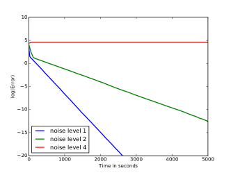
(a) Initialization with in-span noise

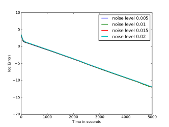
(b) Initialization with out-of-span noise

Figure 3: The performance of the algorithm AND with weak initialization. The $x$-axis is the running time (in seconds), the $y$-axis is the logarithm of the total correlation error. (a) Using different values for the noise level $r_{l}$ that controls the in-span noise in the initialization. (b) Using different values for the noise level $r_{n}$ that controls the out-of-span noise in the initialization.

B.2 Robustness to Sparsity

We performed experiments on the DIR data with different sparsity. In particular, construct a $100\times 5000$ matrix $\mathbb{X}$, where each column is drawn from a Dirichlet prior $D(\mathbf{\alpha})$ on $d=100$ dimension, where $\mathbf{\alpha}=(\alpha/d,\alpha/d,\ldots,\alpha/d)$ for a scalar $\alpha$. Then the dataset is $\mathbb{Y}=\mathbb{A}^{*}\mathbb{X}$. We varied the $\alpha$ parameter of the prior to control the expected support sparsity, and ran the algorithm on the data generated.

Figure 4 shows the results. For $\alpha$ as large as $20$, the algorithm still converges to the ground-truth in exponential rate. When $\alpha=80$ meaning that the weight vectors (columns in $\mathbb{X}$) have almost full support, the algorithm still produces good results, stabilizing to a small relative error at the end. This demonstates that the algorithm is not sensitive to the support sparsity of the data.

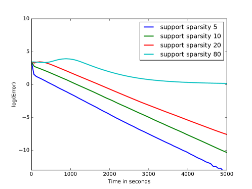
Figure 4: The performance of the algorithm AND on data generated from Dirichlet prior on $x$ with different sparsities. The $x$-axis is the running time (in seconds), the $y$-axis is the logarithm of the total correlation error.

B.3 Qualitative Results on Some Real World Applications

We applied our algorithm to two popular applications with real world data to demonstrate the applicability of the method to real world scenarios. Note that the evaluations here are qualitative, due to that the guarantees for our algorithm is the convergence to the ground-truth, while there are no predefined ground-truth for these datasets in practice. Quantitative studies using other criteria computable in practice are left for future work.

B.3.1 Topic Modeling

Here our method is used to compute $10$ topics on the 20newsgroups dataset, which is a standard dataset for the topic modeling setting. Our algorithm is initialized with $10$ random documents from the dataset, and the hyperparameters like learning rate are from the experiments in the main text. Note that better initialization is possible, while here we keep things simple to demonstrate the power of the method.

Table 1 shows the results of the NMF method and the LDA method in the sklearn package, and the result of our AND method. It shows that our method indeed leads to reasonable topics, with quality comparable to well implemented popular methods tuned to this task.

Method	Topic
NMF (sklearn)	just people don think like know time good make way
	windows use dos using window program os drivers application help
	god jesus bible faith christian christ christians does heaven sin
	thanks know does mail advance hi info interested email anybody
	car cars tires miles 00 new engine insurance price condition
	edu soon com send university internet mit ftp mail cc
	file problem files format win sound ftp pub read save
	game team games year win play season players nhl runs
	drive drives hard disk floppy software card mac computer power
	key chip clipper keys encryption government public use secure enforcement
LDA (sklearn)	edu com mail send graphics ftp pub available contact university
	don like just know think ve way use right good
	christian think atheism faith pittsburgh new bible radio games
	drive disk windows thanks use card drives hard version pc
	hiv health aids disease april medical care research 1993 light
	god people does just good don jesus say israel way
	55 10 11 18 15 team game 19 period play
	car year just cars new engine like bike good oil
	people said did just didn know time like went think
	key space law government public use encryption earth section security
AND (ours)	game team year games win play season players 10 nhl
	god jesus does bible faith christian christ new christians 00
	car new bike just 00 like cars power price engine
	key government chip clipper encryption keys use law public people
	young encrypted exactly evidence events especially error eric equipment entire
	thanks know does advance mail hi like info interested anybody
	windows file just don think use problem like files know
	drive drives hard card disk software floppy think mac power
	edu com soon send think mail ftp university internet information
	think don just people like know win game sure edu

Table 1: Results of different methods computing $10$ topics on the 20newsgroups dataset. Each topic is visualized by using its top frequent words, and each line presents one topic.

B.3.2 Image Decomposition

Here our method is used to compute $6$ components on the Olivetti faces dataset, which is a standard dataset for image decomposition. Our algorithm is initialized with $6$ random images from the dataset, and the hyperparameters like learning rate are from the experiments in the main text. Again, note that better initialization is possible, while here we keep things simple to demonstrate the power of the method.

Figure 5 shows some examples from the dataset, the result of our AND method, and 6 other methods using the implementation in the sklearn package. It can be observed that our method can produce meaningful component images, and the non-negative matrix factorization implementation from sklearn produces component images of similar quality. The results of these two methods are generally better than those by the other methods.

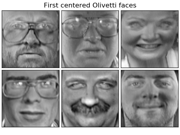
(a) Example images in the dataset

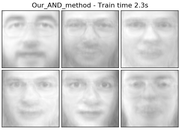
(b) Our AND algorithm

(c) K-means

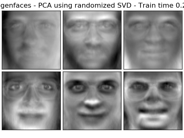
(d) Principal Component Analysis

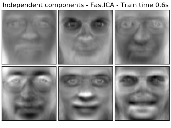
(e) Independent Component Analysis

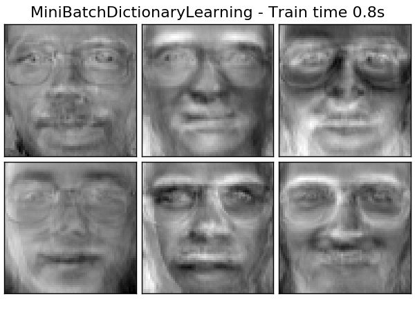
(f) Dictionary learning

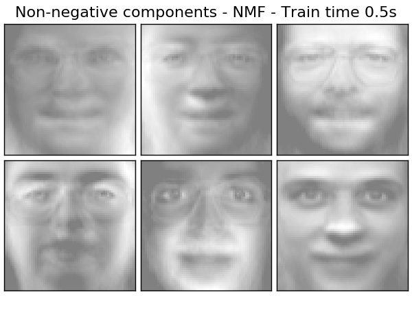
(g) Non-negative matrix factorization (sklearn)

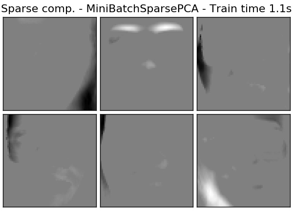
(h) Sparse Principal Component Analysis

Figure 5: The results of different methods computing $6$ components on the Olivetti faces dataset. For all the competitors, we used the implementations in the sklearn package.

References

- lda (2016) Lda-c software. https://github.com/blei-lab/lda-c/blob/master/readme.txt, 2016. Accessed: 2016-05-19.
- Anandkumar et al. (2012) Anandkumar, A., Kakade, S., Foster, D., Liu, Y., and Hsu, D. Two svds suffice: Spectral decompositions for probabilistic topic modeling and latent dirichlet allocation. Technical report, 2012.
- Anandkumar et al. (2013) Anandkumar, A., Hsu, D., Javanmard, A., and Kakade, S. Learning latent bayesian networks and topic models under expansion constraints. In ICML, 2013.
- Arora et al. (2012a) Arora, S., Ge, R., and Moitra, A. Learning topic models – going beyond svd. In FOCS, 2012a.
- Arora et al. (2013) Arora, S., Ge, R., Halpern, Y., Mimno, D., Moitra, A., Sontag, D., Wu, Y., and Zhu, M. A practical algorithm for topic modeling with provable guarantees. In ICML, 2013.
- Arora et al. (2015) Arora, S., Ge, R., Ma, T., and Moitra, A. Simple, efficient, and neural algorithms for sparse coding. In COLT, 2015.
- Arora et al. (2012b) Arora, Sanjeev, Ge, Rong, Kannan, Ravindran, and Moitra, Ankur. Computing a nonnegative matrix factorization–provably. In STOC, pp. 145–162. ACM, 2012b.
- Arora et al. (2016) Arora, Sanjeev, Ge, Rong, Koehler, Frederic, Ma, Tengyu, and Moitra, Ankur. Provable algorithms for inference in topic models. In Proceedings of The 33rd International Conference on Machine Learning, pp. 2859–2867, 2016.
- Awasthi & Risteski (2015) Awasthi, Pranjal and Risteski, Andrej. On some provably correct cases of variational inference for topic models. In NIPS, pp. 2089–2097, 2015.
- Bhattacharyya et al. (2016) Bhattacharyya, Chiranjib, Goyal, Navin, Kannan, Ravindran, and Pani, Jagdeep. Non-negative matrix factorization under heavy noise. In Proceedings of the 33nd International Conference on Machine Learning, 2016.
- Blei & Lafferty (2006) Blei, David and Lafferty, John. Correlated topic models. Advances in neural information processing systems, 18:147, 2006.
- Blei (2012) Blei, David M. Probabilistic topic models. Communications of the ACM, 2012.
- Blei et al. (2003) Blei, David M, Ng, Andrew Y, and Jordan, Michael I. Latent dirichlet allocation. JMLR, 3:993–1022, 2003.
- Cichocki et al. (2007) Cichocki, Andrzej, Zdunek, Rafal, and Amari, Shun-ichi. Hierarchical als algorithms for nonnegative matrix and 3d tensor factorization. In International Conference on Independent Component Analysis and Signal Separation, pp. 169–176. Springer, 2007.
- Ding et al. (2013) Ding, W., Rohban, M.H., Ishwar, P., and Saligrama, V. Topic discovery through data dependent and random projections. arXiv preprint arXiv:1303.3664, 2013.
- Ding et al. (2014) Ding, W., Rohban, M.H., Ishwar, P., and Saligrama, V. Efficient distributed topic modeling with provable guarantees. In AISTAT, pp. 167–175, 2014.
- Hoffman et al. (2010) Hoffman, Matthew, Bach, Francis R, and Blei, David M. Online learning for latent dirichlet allocation. In advances in neural information processing systems, pp. 856–864, 2010.
- Kim & Park (2008) Kim, Hyunsoo and Park, Haesun. Nonnegative matrix factorization based on alternating nonnegativity constrained least squares and active set method. SIAM journal on matrix analysis and applications, 30(2):713–730, 2008.
- Lee & Seung (1997) Lee, Daniel D and Seung, H Sebastian. Unsupervised learning by convex and conic coding. NIPS, pp. 515–521, 1997.
- Lee & Seung (1999) Lee, Daniel D and Seung, H Sebastian. Learning the parts of objects by non-negative matrix factorization. Nature, 401(6755):788–791, 1999.
- Lee & Seung (2001) Lee, Daniel D and Seung, H Sebastian. Algorithms for non-negative matrix factorization. In NIPS, pp. 556–562, 2001.
- Li et al. (2016) Li, Yuanzhi, Liang, Yingyu, and Risteski, Andrej. Recovery guarantee of non-negative matrix factorization via alternating updates. Advances in neural information processing systems, 2016.
- Yang & Leskovec (2013) Yang, Jaewon and Leskovec, Jure. Overlapping community detection at scale: a nonnegative matrix factorization approach. In Proceedings of the sixth ACM international conference on Web search and data mining, pp. 587–596. ACM, 2013.