Waveguides with Absorbing Boundaries: Nonlinearity Controlled by an Exceptional Point and Solitons

Abstract

We reveal the existence of continuous families of guided single-mode solitons in planar waveguides with weakly nonlinear active core and absorbing boundaries. Stable propagation of TE and TM-polarized solitons is accompanied by attenuation of all other modes, i.e., the waveguide features properties of conservative and dissipative systems. If the linear spectrum of the waveguide possesses exceptional points, which occurs in the case of TM polarization, an originally focusing (defocusing) material nonlinearity may become effectively defocusing (focusing). This occurs due to the geometric phase of the carried eigenmode when the surface impedance encircles the exceptional point. In its turn the change of the effective nonlinearity ensures the existence of dark (bright) solitons in spite of focusing (defocusing) Kerr nonlinearity of the core. The existence of an exceptional point can also result in anomalous enhancement of the effective nonlinearity. In terms of practical applications, the nonlinearity of the reported waveguide can be manipulated by controlling the properties of the absorbing cladding.

Localized solutions of one-dimensional (1D) nonlinear conservative guiding systems are known to belong to continuous families characterized by the dependence of the mode intensity on the propagation constant (or frequency, or chemical potential, depending on the physical system). In a broad context such modes are called solitons Dodd . In contrast, localized solutions of nonlinear dissipative 1D systems are isolated points in the functional space. When stable, they are attractors, whose characteristics depend on the system parameters, and are cited as dissipative solitons Akhmediev . While solitons emerge from the balance between the nonlinearity and dispersion, dissipative solitons require also the balance between gain and loss dissipative . There are two known exceptions of this rule. The first one is the parity-time (${\cal PT}$) symmetric Bender systems where the symmetry of the real and imaginary parts of the complex potential ensures the balance between gain and loss without need of additional constraints. Such modes were found for the optical systems governed by the nonlinear Schrödinger (NLS) equation with ${\cal PT}$-symmetric potentials Christodoulides , and are widely investigated in numerous applications spec_issue ; review . The second type of nonconservative systems supporting families of nonlinear modes is a NLS equation with Wadati potentials Wadati , whose conservative part has a specific relation to the gain and loss landscapes Tsoy ; ZK_OL ; review ; YN . This was numerically found in Tsoy , explained in ZK_OL , and in YN it was argued that no other potentials admit soliton families. Conceptually, the coexistence of conservative and dissipative regimes, is also known for dynamical systems described by time-reversible Hamiltonians PoOpBa .

The situation can be different, if a system is not strictly 1D and there exist additional governing parameters. In this Letter we report a wide class of nonlinear waveguides with gain at the core and loss at the cladding, which nevertheless support propagation of continuous families of quasi-1D solitons. The underlying physical idea is a setting where the gain and loss are controlled by different mechanisms affecting the carrier wave itself rather than its envelope. Such a waveguide features properties of an open system: the parameters of solutions are determined by the balance between gain and loss. On the other hand, it supports continuous families of solitons, i.e. obeys properties of a conservative system. Moreover, the type of the nonlinearity of such a system is controlled by the gain and loss. A waveguide with a defocusing (focusing) Kerr dielectric in the core can manifest effective focusing (defocusing) nonlinearity felt by a propagating beam. This effect occurs only if there exists an exceptional point (EP) in the linear spectrum of the waveguide, i.e., the point where two (or more) eigenvalues and eigenfunctions coalesce Kato , and represents a manifestation of the topological geometric phase which is acquired by eigenmodes when encircling the EP in the parameter space geom_phase ; Rotter .

The relevance of EPs in physics was recognized more than a century ago. The Voigt wave Voigt , which is the coalescence of two plane waves propagating in absorbing crystals having singular axes, exists at the EP of the dielectric tensor general-Voigt ; MacLak . Recently, the importance of EPs was demonstrated in experiments with microwave cavities microcav , laser systems EP_laser , waveguides waveguide_EP , multilayered structures multilaiered , and optomechanical systems optomechanical , to mention a few.

If a system is nonlinear, an EP in the spectrum of its linear limit still influences the propagation EP_laser ; Jianke ; ZezKon ; Bludov . However, usually it is not considered as a factor affecting the nonlinear properties of the system itself. In this Letter we show how an EP can modify the effective nonlinearity of the medium, in particular, changing its type.

Consider a planar waveguide consisting of an active medium characterized by the dielectric constant $\epsilon=\epsilon_{r}+i\epsilon_{i}$, with $\epsilon_{r}>0$ and $\epsilon_{i}<0$, which is bounded by two parallel absorbing layers located at the planes $y=\pm\ell$. The medium obeys Kerr nonlinearity and is allowed to have nonlinear absorption (nonlinear gain is treated similarly); i.e., it is described by the Kerr coefficient $\chi_{\!{}_{NL}}=|\chi_{\!{}_{NL}}|e^{i\varphi_{\chi}}$, where $\varphi_{\chi}\in[0,\pi]$ characterizes both the type of the nonlinearity and the relative strength of the nonlinear absorption. The medium is focusing if $\varphi_{\chi}\in[0,\pi/2)$ and defocusing if $\varphi_{\chi}\in(\pi/2,\pi]$. At $\varphi_{\chi}=\pi/2$ the nonlinearity is purely absorbing.

Let ${\bf F}$ be a monochromatic field, either electric ${\bf E}$ or magnetic ${\bf H}$ for TE or TM polarizations, respectively, which is polarized along the $\hat{\bf{x}}$ direction and propagates along the $\hat{\bf{z}}$ direction. It solves the Helmholtz equation

$$\nabla^{2}{\bf F}+\ell^{2}k_{0}^{2}\epsilon~{}{\bf F}+\chi|{\bf F}|^{2}{\bf F}=0$$ (1)

We use the dimensionless variables measuring the coordinates in the units of $\ell$, $k_{0}=\omega/c$, $\omega$ being the frequency, and $\chi=4\pi\chi_{\!{}_{NL}}(\ell k_{0})^{2}$ being the material nonlinearity. To simplify the model, we choose a waveguide whose linear properties were previously studied MK . Namely, we consider that each of the absorbing boundaries is characterized by an impedance $\eta$ and that the fields satisfy the impedance boundary conditions which can be written as Senior ${\bf n\times E}=\eta{\bf H}$, where ${\bf n}$ is the normal to the cladding outwards the waveguide core. This choice is justified when the modulus of the effective dielectric permittivity of cladding is large, $|\epsilon_{\rm{clad}}|\gg 1$.

Because of the active filling, even in the presence of absorbing boundaries one can find waveguide parameters assuring simultaneous guidance of one mode, weak attenuation of a few modes, and strong absorption of all other modes. This selectivity stems from different conditions of balance between gain and loss for modes having different transverse distributions. If a solution of the linear problem, i.e., of Eq. (1) at $\chi=0$, is chosen in the form of a superposition of the guided and weakly decaying modes, an expected effect at weak material nonlinearity, $|\sqrt{\chi}~{}{\bf F}|^{2}\ll 1$, is the existence of solitons.

We show this for a waveguide with one guided and one weakly absorbed mode [see Fig. 1 (a), and Figs. 2(a) and 2(e) below]. The propagating modes are searched in the form $F\sim e^{iqz}\phi(y)$, where $q$ is the propagation constant. The transverse profile of the mode $\phi(y)$ is determined from the non-Hermitian Sturm-Liouville eigenvalue problem $\phi_{yy}=-Q^{2}\phi$ subject to the impedance (alias Robin) boundary conditions: $\phi^{TE}(\pm 1)=\pm\eta^{TE}\phi_{y}^{TE}(\pm 1)$ with $\eta^{TE}=\eta c/(i\omega\ell)$ for TE modes, and $\phi_{y}^{TM}(\pm 1)=\pm\eta^{TM}\phi^{TM}(\pm 1)$ with $\eta^{TM}=i\omega\epsilon\ell\eta/c$ for TM modes. Since the dielectric permittivity and surface impedance are complex, the eigenvalue $Q=Q^{\prime}+iQ^{\prime\prime}$ is complex, as well. Nevertheless, the propagation constant of the guided mode $q=(\ell^{2}k_{0}^{2}\epsilon-Q^{2})^{1/2}$ is real, if

$$\epsilon_{r}>[(Q^{\prime})^{2}-(Q^{\prime\prime})^{2}]/\ell^{2}k_{0}^{2}\quad\mbox{and}\quad\epsilon_{i}=2Q^{\prime}Q^{\prime\prime}/\ell^{2}k_{0}^{2}.$$ (2)

All other modes (marked by the subindex $n$) are absorbed if the condition $Q^{\prime}Q^{\prime\prime}>Q_{n}^{\prime}Q_{n}^{\prime\prime}$ is verified. To distinguish the weakest absorbing mode, below we use a tilde, i.e., $\tilde{\phi}$, $\tilde{Q}$ and $\tilde{q}$. For such a mode $\tilde{q}=(\ell^{2}k_{0}^{2}\epsilon-\tilde{Q}^{2})^{1/2}=\tilde{q}^{\prime}+i\tilde{q}^{\prime\prime}$, where $\tilde{q}^{\prime\prime}>0$, and $|\tilde{q}^{\prime\prime}|\ll|\tilde{q}^{\prime}|$.

We start with a waveguide whose linear spectrum does not feature EPs. Let $\psi(y)$ be an eigenfunction of the Sturm-Liouville problem adjoint to the above one for $\phi(y)$. The states $\{\phi,\tilde{\phi},\phi_{2},\phi_{3},...\}$ and $\{\psi,\tilde{\psi},\psi_{2},\psi_{3},...\}$ constitute a complete biorthogonal basis suppl , which is endowed with the scalar product $\langle\psi,\phi\rangle=\int_{-1}^{1}\psi^{*}(y)\phi(y)dy$. In particular, $\langle\psi,\tilde{\phi}\rangle=\langle\tilde{\psi},\phi\rangle=0$. The eigenfunctions $\psi=\phi^{*}$ and $\tilde{\psi}=\tilde{\phi}^{*}$ correspond to the eigenvalues $Q^{*}$ and $\tilde{Q}^{*}$.

Next, we look for a solution of Eq. (1) in the form $F\approx A(x,z)\phi(y)e^{iqz}+\tilde{A}(x,z)\tilde{\phi}(y)e^{i\tilde{q}z},$ where $A$ and $\tilde{A}$ are the slowly varying amplitudes of the modes. Performing the multiple-scale analysis suppl , we obtain coupled NLS equations

$$2iqA_{z}+A_{xx}+(g|A|^{2}+g_{1}e^{-2\tilde{q}^{\prime\prime}z}|\tilde{A}|^{2})A=0,$$ (3)

$$2i\tilde{q}^{\prime}\tilde{A}_{z}+\tilde{A}_{xx}+(\tilde{g}_{1}|A|^{2}+\tilde{g}e^{-2\tilde{q}^{\prime\prime}z}|\tilde{A}|^{2})\tilde{A}=0,$$ (4)

where the complex nonlinear coefficients describing effective self-phase and cross-phase modulations are

$$\begin{array}[]{ll}g=\chi\langle\psi,|\phi|^{2}\phi\rangle/\langle\psi,\phi\rangle,{}&g_{1}=2\chi{\langle\psi,|\tilde{\phi}|^{2}\phi\rangle}/\langle\psi,\phi\rangle,\\ \tilde{g}=\chi\langle\tilde{\psi},|\tilde{\phi}|^{2}\tilde{\phi}\rangle/\langle\tilde{\psi},\tilde{\phi}\rangle,&\tilde{g}_{1}=2\chi\langle\tilde{\psi},|\phi|^{2}\tilde{\phi}\rangle/\langle\tilde{\psi},\tilde{\phi}\rangle.\end{array}$$ (5)

Since $\tilde{\phi}$ is the most weakly decaying mode, at the propagation distance $z\gtrsim 1/\tilde{q}^{\prime\prime}$ the effect of all decaying modes on the guided one, i.e. on $A$, can be neglected. After that distance the guided mode $\phi$ is the only one, which propagates with the amplitude governed by the NLS Eq. (3) with $\tilde{A}=0$. This however, does not guarantee yet undistorted propagation because generally speaking $g$ is complex. In order to obtain the conservative NLS equation, which is exactly integrable and thus possesses soliton (as well as multi-soliton) solutions Dodd , we additionally have to require $g$ to be real. To this end we define the argument $\varphi_{g}=\arg\left(\langle\psi,|\phi|^{2}\phi\rangle/\langle\psi,\phi\rangle\right)\in[-\pi,\pi]$. Then Eq. (3) with $\tilde{A}=0$ becomes the conservative NLS equation only if either $\varphi_{\chi}=-\varphi_{g}$ at $\varphi_{g}\in[-\pi,0]$ or $\varphi_{\chi}=\pi-\varphi_{g}$ at $\varphi_{g}\in[0,\pi]$ is satisfied. This leads us to several interesting conclusions.

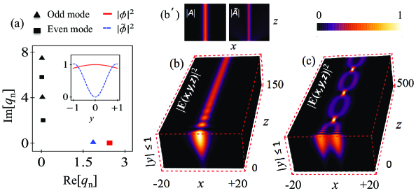
Figure 1: (a) Real part vs imaginary part of the propagation constants for the waveguide with $\eta^{TE}=-1.25-3.16i$, $\epsilon=1.5-0.062i$, $|\chi_{\!{}_{NL}}|=0.025$ and $k_{0}\ell=2\pi/3.1$. Squares and triangles represent the $\cos(Qy)-$ and $\sin(Qy)-$modes, respectively. The guided and weakest decaying modes are indicated by red and blue color, respectively; their transverse profiles are shown in the inset. (b) Dynamics of the single bright TE-soliton input $A=2\tilde{A}=0.5\operatorname{sech}(\sqrt{g/8}x)$ with the amplitude profiles shown in (b^′) (see also suppl ). (c) Dynamics of the in-phase two-soliton input: $A=2\tilde{A}=0.5[\operatorname{sech}(\sqrt{g/8}(x+5))+\operatorname{sech}(\sqrt{g/8}(x-5))]$. The effective nonlinearities are $g=1.24$, $\tilde{g}=1.02+0.02i$, $g_{1}=1.34+0.07i$, $\tilde{g}_{1}=2.4+0.002i$. Simulations were carried out on the window $-200<x<200$ and $0<z<1000$. The inputs were perturbed by noise of order 5% of the amplitude.

First, if the total phase $\varphi=\varphi_{\chi}+\varphi_{g}$ of the effective nonlinearity $g$ is either $0$ or $\pi$ the absorbing boundaries may support propagation of a single-mode soliton, by attenuating all other modes. Second, since solitons of the NLS equation constitute two-parametric families Dodd , they are characterized by amplitudes and by velocities, the waveguide supports continuous families of the propagating spatially localized beams, i.e. behaves in this respect like a conservative system. Third, it is possible to choose the waveguide parameters such that the effective nonlinearity $g$ for a guided mode has opposite signs compared to the sign of the physical nonlinearity $\chi$ of the waveguide core. Specifically, for the nonlinear absorption considered here we have

$$\begin{array}[]{ll}g>0\quad\mbox{ and}\quad\mbox{ Re$\,\chi<0$}\quad\mbox{if $\varphi_{g}\in[-\pi,-\frac{\pi}{2}]$},\\ g<0\quad\mbox{ and}\quad\mbox{ Re$\,\chi>0$}\quad\mbox{if $\varphi_{g}\in[\frac{\pi}{2},\pi]$}.\end{array}$$ (8)

Thus the combined effect of the (linear) boundary absorption with (linear) gain of the active media may result in the change of the type of the effective nonlinearity. Then focusing (defocusing) material nonlinearity of the core becomes effectively defocusing (focusing). Consequently, this may result in the guidance of bright (dark) solitons even in the defocusing (focusing) material nonlinearity of the dielectric filling.

Now we turn to examples of waveguide architecture supporting soliton propagation. The consideration will be restricted to nonmagnetic claddings characterized by the positive dielectric constant, $\epsilon_{\rm clad}>0$, which corresponds to natural materials (see Ref. MK for examples). This last requirement imposes conditions on the effective impedances MK : $\mbox{Re}~{}\eta^{TE},~{}\mbox{Im}~{}\eta^{TE}~{}<~{}0$, and $\mbox{Re}~{}\eta^{TM},~{}\mbox{Im}~{}\eta^{TM}~{}>~{}0$. The desired parameters can be achieved by adjusting the wave number $k_{0}$, the waveguide width $\ell$, the nonlinear susceptibility, $\chi_{\!{}_{NL}}$, and the impedance $\eta$. The dielectric permittivity is not considered as an adjustable parameter, because the condition of mode guiding [Eq. 2] fixes it as soon as the respective impedance is chosen.

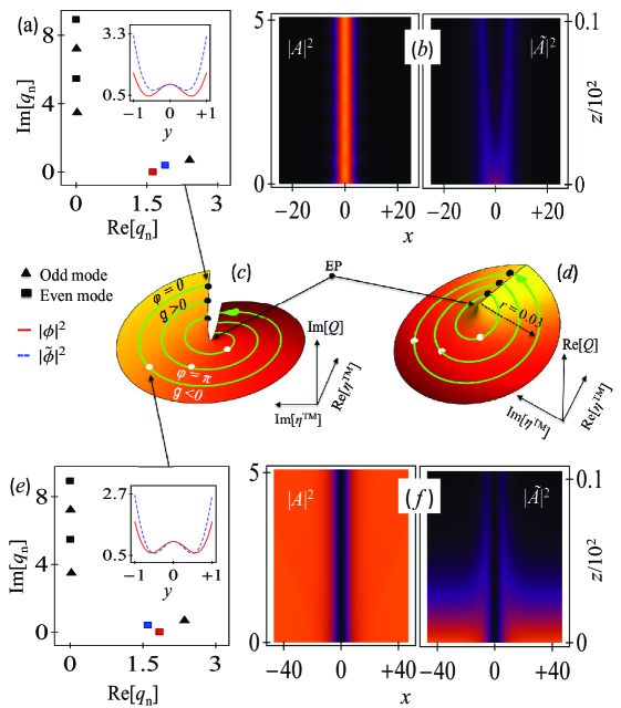
Figure 2: Central panels: Imaginary (c) and real (d) parts of the eigenvalue $Q$ corresponding to a TM-mode in the vicinity of EP, $\eta^{EP}=1.6506+2.05998i$, vs real and imaginary parts of the impedance, for $0<r<0.04$ and $0\leq\Theta\leq 2\pi$. The mode is chosen to be guided at two values of the total phase $\varphi$: at black discs $\Theta=0$, $\varphi=0$ and $g>0$, while white discs represent the same points after change of the impedance resulting in $\varphi=\pi$ and $g<0$. The positions of the phase changes are shown at $(r,\Theta)=(0.01,1.25\pi),(0.02,0.91\pi)$ and $(0.03,0.722\pi)$, when $\chi=0.12+1.29i,0.61+1.14i$, and $0.87+0.95i$, respectively. Different $\chi$ for different radii ensure that $g$ is real at both white and black points. Upper panels: (a) Propagation constants, and profiles of the guided and weakly decaying TM modes (in the inset), and (b) dynamics of a bright TM-soliton with $A=2\tilde{A}=0.5\operatorname{sech}(\sqrt{g/8}x)$ at the input, for $g=1.42$ at $r=0.03$ [black discs in (c) and (d)] observed for $\eta^{TM}=1.681+2.060i$, $\epsilon=1.5-0.986i$, $q=1.63$, and $\tilde{q}=1.897+0.386i$. Lower panels: (e) Propagation constants, and the guided and weakly decaying modes (in the inset) and (f) dynamics of a dark TM-soliton excited by the $A=2\tilde{A}=0.5\tanh(\sqrt{|g|/8}x)$ input for $g=-0.073$ at $r=0.03$ [white discs in (c) and (d)] obtained for $\eta^{TM}=1.631+2.083i$, $\epsilon=1.5-0.999i$, $q=1.85$, and $\tilde{q}=1.609+0.409i$. In all panels $k_{0}\ell=2\pi/3.1$. Simulations were carried out on the window $-200<x<200$ and $0<z<1000$. Inputs were perturbed by noise of order 5% of the amplitude.

TE soliton – For TE-polarized modes, we have found that gain and loss do not change the sign of the effective nonlinearity in the whole domain of the explored parameters. Figure 1(a) illustrates propagation constants for the parameter choice ensuring the existence of one guided (red square) and one weakly absorbed (blue triangle) mode. All other modes (the lowest ones are shown in black) are strongly absorbed. The transverse profile of the fundamental (guided) mode is given by $\phi(y)=\cos(Qy)$ with $Q\approx 0.453-0.279i$, and the propagation constant is $q\approx 2.457$. We also compute $\varphi_{g}\approx-0.0027$ and, hence, one has to choose $\chi=1.3+0.0035i$, in order to ensure real $g$. The transverse profile of the weakly decaying mode is described by $\tilde{\phi}(y)=\sin(\tilde{Q}y)$, where $\tilde{Q}\approx 1.65-0.158i$, and $\tilde{q}\approx 1.86+0.073i$.

The direct numerical simulations of Eqs. (3) and (4), are shown in Figs. 1 (b)–(c). In Fig. 1 (b) we observe stable propagation of a single soliton carried by the fundamental mode after the second mode is absorbed by the structure (this is clearly visible on the 3D figure), while the upper inset shows nondecaying evolution of the soliton $A$, and an accompanying mode soliton $\tilde{A}$ (after the distance $z\gtrsim 1/\tilde{q}^{\prime\prime}$ the soliton is not affected by the decaying mode, because Eqs. (3) and (4) become effectively decoupled). In Fig. 2 (c) we show the evolution of the two-soliton input (each input soliton consists of carrying and weakly decaying modes). After decay of the accompanying mode we observe the characteristic dynamics of interacting in-phase solitons (i.e., of a breather) (cf. two-soliton , see also Ref. suppl ).

TM soliton – In the spectrum of TM modes there can exist EPs MK . This makes the properties of TM modes very different as compared with TE-modes considered above. Let the impedance $\eta^{TM}$ be chosen in the vicinity of an EP, i.e., $\eta^{TM}=\eta^{EP}+re^{i\Theta}$, where $r\ll 1$ (for a given statement $\eta^{EP}$ has a specific numerical value, but can be varied by modifying setting of the problem suppl ). Although, strictly speaking the small amplitude expansion leading to Eqs. (3) and (4) fails in the neighbourhood of $\eta^{EP}$, we are interested exclusively in the phase behavior. Then, taking into account that at EP two eigenvalues coalesce, one can expand $Q\approx Q^{EP}+\nu e^{i\vartheta}$ where $\nu\sim\sqrt{r}\ll 1$ is a small parameter, while $\vartheta=\Theta/2+\vartheta_{0}$, where $\vartheta_{0}=$const, is the phase which is changed by $\pi$ when $\eta^{TM}$ encircles the EP, i.e., when $\Theta$ is changed by $2\pi$. Let the coalescing modes be of cosine type, i.e. $\phi(y)=\cos(Qy)$. Then in the leading order of the effective nonlinearity $g$ takes the form

$$g\approx-\chi e^{-i\vartheta}\frac{\int_{-1}^{1}\cos^{2}(Q^{EP}y)|\cos(Q^{EP}y)|^{2}dy}{\nu\int_{-1}^{1}y\sin(2Q^{EP}y)dy}.$$ (9)

Here we used the self-orthogonality of the eigenfunctions in the EP (see e.g. Rotter ): $\int_{-1}^{1}\cos^{2}(Q^{EP}y)dy=0$. Thus $\varphi_{g}=-\vartheta+$const and the argument of $g$ changes by $\pi$ when $\eta^{TM}$ encircles $\eta^{EP}$. According to the conditions (8) this means that the type of the effective nonlinearity changes (form focusing to defocusing or vice versa) independently of the material nonlinearity $\chi$.

If $Q$ is located away from the EP, the total phase $\varphi$ becomes nonlinearly dependent on the rotation angle $\Theta$. This dependence in function of the “distance” $r$ between $\eta^{TM}$ and the EP is illustrated in two central panels of Fig. 2. In the figure the change of the rotation angle $\Theta$ corresponds to the “motion” along the curves in the direction indicated by arrows. The striking situation of the opposite signs of the physical and effective nonlinearities is observed when the parameters “move” from black discs (Re$\,\chi>0$, $g>0$) to the white discs (Re$\,\chi>0$, $g<0$). With the increase of $r$ the smaller rotation angle $\Theta$ is needed to achieve the total-phase change $\pi$. At the cladding impedance $\eta^{TM}$ corresponding to the black discs the effective nonlinearity is focusing and bright solitons can propagate in the system. An example is shown in the upper panels of Fig. 2. We observe very robust evolution of the guided mode, even if at the input a weakly decaying mode is excited as well. Now the weakly decaying mode has the same parity as the guided one [shown by red and blue squares in Fig. 2(a)] since both of them coalesce in the EP. The energy carried by both modes is concentrated near the absorbed boundaries. Unlike in the TE case, now the guided mode is not the fastest one: the largest positive propagation constant belongs to the decaying sine mode [the right triangle in Fig. 2 (a)].

When the physical and effective nonlinearities are of different signs, in a waveguide with focusing nonlinearity there can propagate a stable dark soliton. In Fig. 2 this is the situation corresponding to the white discs in panels (c) and (d). The stable evolution of a guided dark soliton excited at the input together with weakly decaying dark soliton, is illustrated in Fig. 2(f). Interestingly, while the structure of the modes remains similar to that of the bright soliton obtained for the same nonlinearity now the guided and weakly decaying modes are “exchanged” [c.f. the insets and the location of red and blue squares in Figs. 2(a) and  2(e)]. Similarly one can design a waveguide with defocusing core nonlinearity supporting the propagation of bright TM polarized solitons. Finally, we mention the possibility of anomalous enhancement of the nonlinearity, which stems from the non-Hermitian nature of the system allowing the inner product $\langle\psi,\phi\rangle$ to be infinitely small which leads to anomalously large effective nonlinearity $g$, seen from Eqs. (5) and (9) where $g\to\infty$ at $\nu\to 0$ suppl .

In conclusion, we reveal the key features of a dissipative waveguide with a nonlinear active core and absorbing boundaries which allow for the propagation of single-mode solitons and attenuate all other modes excited at the input. The type of the effective nonlinearity (focusing vs defocusing), as well as its absorbing or active characteristics are controlled by the boundary conditions. If the spectrum of the linear modes features EPs, the effective nonlinearity may acquire a sign opposite to the sign of the material nonlinearity of the core, which stems from the geometric phase acquired by the eigenfunctions when the impedance encircles the EP. In such situations the focusing (defocusing) Kerr nonlinearity can support propagation of dark (bright) solitons. The solitons reported are structurally stable: the dependence on the waveguide parameters is continuous under the change of the parameters assuring the existence of the guided mode, while weak deviation of the parameters from the ideal guiding conditions results only in weak net dissipation or gain. An important practical output, is that in the reported structures the sign of the effective nonlinearity can be changed in situ when the physical characteristics of the boundary are changed (by remote similarity with the atomic physics, where the change of the nonlinearity type is achieved by the Feshbach resonance). Although we used the impedance boundary conditions, the reported effects are accessible with other types of absorbing boundaries and other types of dielectric filling. In particular, by using cladding with different impedances or made of metasurfaces meta , or birefringent filling one can control the position of the EP in the complex plane.

Supplemental material

.1 Derivation of the paraxial approximation Eqs. (3), (4)

For the sake of completeness, here we present a complete formal derivation of the paraxial approximation [Eqs. (3) and (4) of the main text] for the case of Robin boundary conditions. The derivation is given for the TE wave (for TM the derivation is similar).

Let us start with

$$\nabla^{2}E+\ell^{2}k_{0}^{2}\epsilon E+\chi|E|^{2}E=0.$$ (S1)

and introduce the formal small parameter $\mu\ll 1$ defining the expansion for the field amplitude:

$$E=\mu E_{0}+\mu^{2}E_{1}+\mu^{3}E_{2}+\cdots$$ (S2)

as well as the scaled variables $\{x_{0},x_{1},...\}$ and $\{z_{0},z_{1},...\}$ with $x_{j}=\mu^{j}x$ and $z_{j}=\mu^{j}z$, which are treated as independent, so that

$$\frac{\partial}{\partial x}=\frac{\partial}{\partial x_{0}}+\mu\frac{\partial}{\partial x_{1}}+\cdots\,,\quad\frac{\partial}{\partial z}=\frac{\partial}{\partial z_{0}}+\mu\frac{\partial}{\partial z_{1}}+\cdots$$ (S3)

Substitution (S2) and (S3) in Eq. (S1) we obtain a series of equations at different orders of $\mu$

$$\mu=1:\quad {\mathcal{L}}E_{0}=0,\qquad{\mathcal{L}}\equiv\nabla_{0}^{2}+\ell^{2}k_{0}^{2}\epsilon,$$ (S4)

$$\mu=2:\quad {\mathcal{L}}E_{1}=2\frac{\partial^{2}E_{0}}{\partial x_{0}\partial x_{1}}+2\frac{\partial^{2}E_{0}}{\partial z_{0}\partial z_{1}},$$ (S5)

$$\mu=3:\quad {\mathcal{L}}E_{2}=2\frac{\partial^{2}E_{1}}{\partial x_{0}\partial x_{1}}+2\frac{\partial^{2}E_{1}}{\partial z_{0}\partial z_{1}}+\frac{\partial^{2}E_{0}}{\partial x_{1}^{2}}+\frac{\partial^{2}E_{0}}{\partial z_{1}^{2}}$$ (S6)

$$\quad\quad+2\frac{\partial^{2}E_{0}}{\partial x_{0}\partial x_{2}}+2\frac{\partial^{2}E_{0}}{\partial z_{0}\partial z_{2}}+\chi|E_{0}|^{2}E_{0},$$

where (notice that for the $y$-variables no scaling is needed)

$$\nabla_{0}\equiv\left(\frac{\partial}{\partial x_{0}},\frac{\partial}{\partial y},\frac{\partial}{\partial z_{0}}\right).$$

Consider now the Sturm-Liouville eigenvalue problem

$$\phi_{yy}=-Q^{2}\phi,\quad{\phi(\pm 1)=\pm\eta^{TE}\phi_{y}(\pm 1)},$$ (S7)

and its conjugate

$$\psi_{yy}=-\tilde{Q}^{2}\psi,\quad{\psi(\pm 1)=\pm{(\eta^{TE})}^{*}\psi_{y}(\pm 1)}.$$ (S8)

Let us define

$$q=\left(\ell^{2}k_{0}^{2}\epsilon-Q^{2}\right)^{1/2}=q^{\prime}+i\mu q^{\prime\prime},$$ (S9)

where $q^{\prime},q^{\prime\prime}$ are real and the branch is chosen to ensure $q^{\prime}\geq 0$. As a matter of fact (S9) reveals also the physical sense of the small parameter: it is a relation of the gain/loss coefficient to the propagation constant (in the original physical units). The spectra of the above Sturm-Liouville problems are discrete, and the eigenfunctions constitute the sets: $\{\phi_{0},\phi_{1},\phi_{2}...\}$ and $\{\psi_{0},\psi_{1},\psi_{2}...\}$, respectively. We can choose the numbering of the eigenfunction $\phi_{n}$ and the respective eigenvalues $Q_{n}$ such that $q_{n}^{\prime\prime}=\mbox{Im}(q_{n})$ are ordered as

$$q_{0}^{\prime\prime}<q_{1}^{\prime\prime}<q_{2}^{\prime\prime}<\cdots$$ (S10)

Then the set for $\psi_{n}$ is determined by: $\psi_{n}=\phi_{n}^{*}$. Obviously, this ordering corresponds to higher modes undergoing stronger attenuation (or weaker amplification if the lowest $q_{n}$ are negative, this case however will not be considered here).

It is straightforward to ensure that

$$\langle\psi_{n},\phi_{m}\rangle=\int_{-1}^{1}\psi_{n}^{*}(y)\phi_{m}(y)dy=0\quad\mbox{if $m\neq n$}.\quad$$ (S11)

Let us now assume that at the input, i.e. at $z=0$, only the two lowest modes, $\phi_{0}$ and $\phi_{1}$ are excited. Respectively we look for a solution of (S1) in the form where

$$E_{0}=A_{0}\phi_{0}(y)e^{iq_{0}^{\prime}z_{0}-q_{0}^{\prime\prime}z_{2}}+A_{1}\phi_{1}(y)e^{iq_{1}^{\prime}z_{0}-q_{1}^{\prime\prime}z_{2}},\quad\quad$$ (S12)

where $A_{0}$ and $A_{1}$ are functions of only slow variables $x_{1},\,x_{2},...$ and $z_{1},\,z_{2},...$. The relation (S9) ensures, that the so defined $E_{0}$ solves (S4).

Turning to the second order of the expansion. A general from of $E_{1}$, which at the input is zero, now reads (since we are considering the parameters out of the exceptional point, the sets $\{\phi_{0},\phi_{1},\phi_{2},...\}$ and $\{\psi_{0},\psi_{1},\psi_{2},...\}$ constitute a biorthogonal basis):

$$E_{1}=\sum_{m\neq 0}B_{m}^{(0)}\phi_{m}(y)e^{iq_{0}^{\prime}z_{0}}+\sum_{m\neq 1}B_{m}^{(1)}\phi_{m}(y)e^{iq_{1}^{\prime}z_{0}},$$ (S13)

where $B_{m}^{(0)}$ and $B_{m}^{(1)}$ are functions on slow variables only. Since $E_{1}=0$ at $z=0$ and we are looking for a solution independent on $x_{0}$ one ensures that (S5) is satisfied by all $B_{m}^{(0,1)}=0$ and $\partial A_{0,1}/\partial z_{1}=0$. Thus $E_{1}\equiv 0$, and $A_{0,1}=A_{0,1}(x_{1},z_{2})$, i.e. depend on $x_{1},\,x_{2},...$ and $z_{2},\,z_{3},...$.

Turning now to the third order in $\mu$, we compute the right hand side of (S6) in the form

$${\mathcal{L}}E_{2}=\phi_{0}e^{iq_{0}^{\prime}z_{0}-q_{0}^{\prime\prime}z_{2}}\left(2iq_{0}^{\prime}\frac{\partial A_{0}}{\partial z_{2}}+\frac{\partial^{2}A_{0}}{\partial x_{1}^{2}}\right)$$

$$+\phi_{1}e^{iq_{1}^{\prime}z_{0}-q_{1}^{\prime\prime}z_{2}}\left(2iq_{1}^{\prime}\frac{\partial A_{1}}{\partial z_{2}}+\frac{\partial^{2}A_{1}}{\partial x_{1}^{2}}\right)$$

$$+\chi e^{iq_{0}^{\prime}z_{0}}\phi_{0}\left(e^{-2q_{0}^{\prime\prime}z_{2}}|\phi_{0}|^{2}|A_{0}|^{2}+2e^{-2q_{1}^{\prime\prime}z_{2}}|\phi_{1}|^{2}|A_{1}|^{2}\right)A_{0}$$

$$+\chi e^{iq_{1}^{\prime}z_{0}}\phi_{1}\left(2e^{-2q_{0}^{\prime\prime}z_{2}}|\phi_{0}|^{2}|A_{0}|^{2}+e^{-2q_{1}^{\prime\prime}z_{2}}|\phi_{1}|^{2}|A_{1}|^{2}\right)A_{1}$$

$$+e^{i(2q_{0}^{\prime}-q_{1}^{\prime})z_{0}}e^{-(2q_{0}^{\prime\prime}+q_{1}^{\prime\prime})z_{2}}\phi_{0}^{2}\phi_{1}^{*}A_{0}^{2}A_{1}^{*}$$

$$+e^{i(2q_{1}^{\prime}-q_{0}^{\prime})z_{0}}e^{-(2q_{1}^{\prime\prime}+q_{0}^{\prime\prime})z_{2}}\phi_{1}^{2}\phi_{0}^{*}A_{1}^{2}A_{0}^{*}.\quad$$ (S14)

The solvability of this equation requires

$$\langle\psi_{0},{\mathcal{L}}E_{2}\rangle=\langle\psi_{1},{\mathcal{L}}E_{2}\rangle=0.$$ (S15)

Now considering the lowest mode with $q_{0}^{\prime\prime}=0$, and denoting $q_{0}=q,q_{1}=\tilde{q}$, $\phi_{0}=\phi$ and $\phi_{1}=\tilde{\phi}$, using the orthogonality relation, collecting terms having the same propagation constant, i.e. the ones $\sim e^{iq_{0}^{\prime}z_{0}}$ and $\sim e^{iq_{1}^{\prime}z_{0}}$, and letting $\mu=1$ (this does not violate the assumption made at the beginning, provided we scale the slow dependencies properly, i.e. all having the same order), from (S15) we obtain the two nonlinear Schrödinger equations (3) and (4) from the main text.

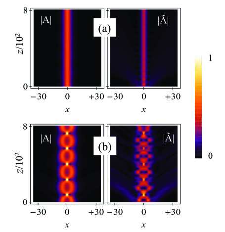
Figure S1: TE soliton mode intensities obtained after simulation of the coupled NLS equation (3) and (4) of the main text. $A$ and $\tilde{A}$ shown in (a) corresponds to soliton 1(b) of main text; and those shown in (b) correspond to soliton 1(c) of main text. Dynamics are done for the initial inputs : (a) $A(x)=2\tilde{A}(x)=0.5\operatorname{sech}(\sqrt{g/8}x)$, and (b) $A(x)=2\tilde{A}(x)=0.5[\operatorname{sech}(\sqrt{g/8}(x+5))+\operatorname{sech}(\sqrt{g/8}(x-5))]$. All the parameters are kept fixed as in Fig. 1 of the main text.

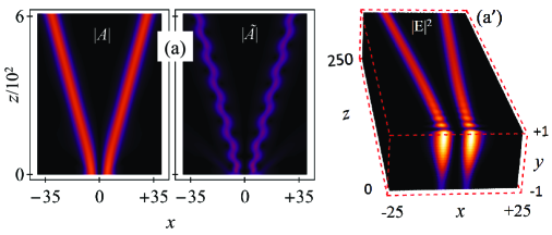
Figure S2: Simulation result for the TE soliton when two humped input solitons placed at $x=\pm 5$ and having relative initial phase $\pi$. In (a) mode amplitudes, and in (a^′) total electric field intensity are shown. All the parameters are kept fixed as in Fig. 1 of the main text.

Ensuring solvability of the Eq. (S6), the small amplitude perturbations of the two lowest modes is searched [by analogy with (S13)] in the form

$$E_{2}=\sum_{m\neq 0}C_{m}^{(0)}\phi_{m}(y)e^{iq_{0}^{\prime}z_{0}}+\sum_{m\neq 1}C_{m}^{(1)}\phi_{m}(y)e^{iq_{1}^{\prime}z_{0}}+$$

$$\sum_{m}\left[D_{m}^{(0)}\phi_{m}(y)e^{i(2q_{0}^{\prime}-q_{1}^{\prime})z_{0}}+D_{m}^{(1)}\phi_{m}(y)e^{i(2q_{1}^{\prime}-q_{0}^{\prime})z_{0}}\right]\quad\quad~{}$$ (S16)

where $C_{m}^{(0,1)}$ and $D_{m}^{(0,1)}$ are functions of slow variables. We are not interested here in the specific form of these coefficients, but a relevant fact is that by formally accounting for all harmonics in (.1), the derivation assures that the approximation well describe the beam evolution of the lowest modes, provided the scaling of the applied beam is properly chosen.

A characteristic feature of the system (3), (4) from the main text, is that it includes decaying terms. In the main text we have shown that, in spite of this signature of the absorbing boundaries, the dynamics of the lowest modes is nearly integrable. This is also visible on the Fig. S1 where we show the evolutions of the the mode intensities, $A(x,z)$ and $\tilde{A}(x,z)$, corresponding to Figure 1 of main text. As an additional confirmation of this fact, in Fig. S2 we illustrate ”repulsion” of two beams having identical intensities and the $\pi$-shifted phases. The observed dynamics closely resemble the dynamics of two out-of-phase solitons of the NLS equation.

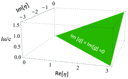
Figure S3: Existence region for non-diffracting (Im$[g]=0$) and non-vanishing (Im$[q]=0$) soliton which was elaborated in the figure 1 of main text. Other parameters for this plot was kept fixed as in figure 1 of main text.

Furthermore, it is important to mention here that the soliton shown in Figure 1 of the main text is point like in the effective parameter space. However, as we show below (in Fig. S3), the corresponding soliton persists for a wide range of physical parameters e.g. actual impedance $\eta$, $\ell$, and $\omega$, which are possible to control in experiments. Moreover, if admit that the condition for the main mode are not perfectly conducting, but result in weak absorption or gain, i.e. in a complex $q_{0}$, the phenomenon is still observable after the respective loss or gain described by $e^{-q_{0}^{\prime\prime}z}$ is scaled out. In this sense the phenomena reported in the main text are structurally stable.

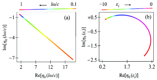
Figure S4: Trajectory of the EP, $\eta_{0}$, in the complex $\eta$ plane with respect to the variation (range of variations are shown in the color bars placed above the respective figure) of (a) $\ell\omega/c$ when $\epsilon=(1.5-0.5~{}i)$ is kept fixed; and (b) gain distribution $\epsilon_{i}$ of the core, when $\epsilon_{r}=1.5$, $\omega=c/2\ell$.

.2 Control of exceptional point by the system parameters

As reported in Ref. MK , the system has infinitely many exceptional points which are defined in the complex effective impedance parameter,$\eta^{TM}$, plane. The effective impedance is a composite parameter consisting of all the physical parameters: $\eta^{TM}=i\eta\omega\epsilon\ell/c$. When expressed in terms of physical impedance $\eta$, the EP can be controlled by changing waveguide transverse dimension, $\ell$, or the frequency, $\omega$, of the incident field, or the dielectric constant, $\epsilon$, of the core. Here in Fig. S4, we show the movement of the EP (for which $\eta^{TM}\approx 1.65061+2.05998i$) in the complex $\eta$ plane for some variation of other parameters. In the figure we denote $\eta_{0}$ as the EP corresponding to the the parameter $\eta$.

A highly promising way of manipulating the parameters of the exceptional point is the use birefringent feeling, changing the relations between the “transverse”, $Q$, and the “forward”, $q$, propagation constants for the mode, which in the meantime add additional control parameters. This possibility requires more extending study.

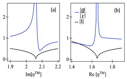
Figure S5: (a) Absolute value of $g$ (in the unit of $|\chi|$) vs Im[$\eta^{TM}$] when Re[$\eta^{TM}]=$ Re$[\eta^{EP}]=1.65$ is fixed; (b) absolute value of $g$ vs Re[$\eta^{TM}$] when Im[$\eta^{TM}]=$ Im$[\eta^{EP}]=2.06$ is fixed. The associated self-overlap integrals are shown black lines.

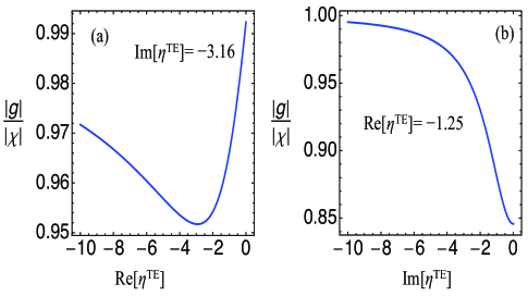
Figure S6: (a) Absolute value of $g$ vs Re[$\eta^{TE}$] when Im[$\eta^{TE}]=-3.16$ is fixed; (b) absolute value of $g$ vs Im[$\eta^{TE}$] when Re[$\eta^{TE}]=-1.25$ is fixed.

.3 Anomalous enhancement of effective-nonlinearity near EP

At an EP, the eigenfunctions of the coalescent mode is self-orthogonal, i.e. $I=\langle\psi,\phi\rangle=\int_{-1}^{1}dy~{}\phi^{2}(y)\to 0$ when $\phi(y)$ approaches the the EP. This in turn implies that the effective nonlinearity $g$ [obtained in eq.(5) of main text] undergoes anomalous enhancement, because vanishing denominator, when the mode approaches an EP. In Fig. S5, we show the numerical evidence of this enhancement, and associated self-overlap integrals when the impedance parameter varies near an EP.

On the other hand, for the TE modes the changes of effective nonlinearity is shown in figure S6, which shows that both enhancement and decrement of effective nonlinearity are also possible.

References

- (1) See e.g. R. K. Dodd, J. C. Eilbeck, J. D. Gibbon, and H. C. Morris, Solitons and Nonlinear Wave Equations (Academic Press, Inc. 1982); A. C. Newell, Solitons in Mathematics and Physics, (Society for Industrial and Applied Mathematic, 1985); A. Scott, Nonlinear Science: Emergence and Dynamics of Coherent Structures (University Press, Oxford, 1999).
- (2) See e.g. V. I. Nekorkin and M. G. Velarde, Synergetic Phenomena in Active Lattices. Patterns, Waves, Solitons, Chaos (Springer-Verlag Berlin heidelberg, 2002); Dissipative Solitons, edited by N. Akhmediev and A. Ankiewicz (Springer-Verlag, Berlin, 2005); M. Tlidi, T. Kolokolnikov, and M. Taki, Focus Issue on Dissipative Localized Structures in Extended Systems, Chaos 17 (2007); M. Tlidi, K. Staliunas, K. Panajotov, A. G. Vladimirov, and M. G. Clerc, Special issue on Localized structures in dissipative media: from optics to plant ecology, Phil. Trans. R. Soc. A 372 (2014).
- (3) M. C. Cross and P. C. Hohenberg, Pattern formation outside of equilibrium, Rev. Mod. Phys. 65, 851 (1993); N. Akhmediev and A. Ankiewicz, Dissipative Solitons in the Complex Ginzburg-Landau and Swift-Hohenberg Equations, in Dissipative Solitons, edited by N. Akhmediev and A. Ankiewicz (Springer-Verlag, Berlin, 2005) p. 1
- (4) C.M. Bender and S. Boettcher, Real Spectra in Non-Hermitian Hamiltonians Having -Symmetry, Phys. Rev. Lett. 80, 5243 (1998); C. M. Bender, Making sense of non-Hermitian Hamiltonians, Rep. Prog. Phys. 70, 947 (2007).
- (5) Z. H. Musslimani, K. G. Makris, R. El-Ganainy, and D. N. Christodoulides, Optical Solitons in Periodic Potentials, Phys. Rev. Lett. 100, 030402 (2008).
- (6) See. e.g. Special issues 3 and 4 of Studies in Applied Mathematics 133, (2014), edited by V. V. Konotop; Focus on Parity-Time Symmetry in Optics and Photonics, New. J. Phys. 18 (2016) edited by D. Christodoulides, R. El-Ganainy, U. Peschel and S. Rotter; Special Issue “Parity-Time Symmetry in Optics and Photonics”, Symmetry 8 (2016), edited by B. M.l Rodríguez-Lara; Non-Hermitian Hamiltonians in Quantum Physics, edited by F. Bagarello, R. Passante, and C. Trapani (Springer International Publishing Switzerland, 2016).
- (7) V. V. Konotop, J. Yang, and D. A. Zezyulin, Nonlinear waves in -symmetric systems. Rev. Mod. Phys. 88, 035002 (2016).
- (8) M. Wadati, Construction of parity-time symmetric potential through the soliton theory. J. Phys. Soc. Jpn. 77, 074005 (2008).
- (9) E. N. Tsoy, I. M. Allayarov, and F. Kh. Abdullaev, Stable localized modes in asymmetric waveguides with gain and loss, Opt. Lett. 39, 4215 (2014).
- (10) V. V. Konotop and D. A. Zezyulin, Families of stationary modes in complex potentials. Opt. Lett. 39, 5535 (2014).
- (11) S. Nixon and J. Yang, All-real spectra in optical systems with arbitrary gain and loss distributions, Phys. Rev. A 93, 031802 (2016); J. Yang and S. Nixon, Stability of soliton families in nonlinear Schrödinger equations with non-parity-time-symmetric complex potentials. Phys. Lett. A 380, 3803 (2016).
- (12) A. Politi, G. L. Oppo, and R. Badii, Coexistence of conservative and dissipative behavior in reversible dynamical systems. Phys. Rev. A 33, 4055 (1986); E. G. Altmann, G. Cristadoro, and D. Pazo, Nontwist non-Hamiltonian systems. Phys. Rev. E 73, 056201 (2006); J. C. Sprott, A dynamical system with a strange attractor and invariant tori, Phys. Lett. A 378, 1361 (2014).
- (13) T. Kato, Perturbation Theory for Linear Operators (Springer-Verlag, Berlin, 1966).
- (14) M. Müller and I. Rotter, Exceptional points in open quantum systems, J. Phys. A: Math. Theor. 41 244018 (2008); U. Günther, I. Rotter, and B. F. Samsonov, Projective Hilbert space structures at exceptional points, J. Phys. A: Math. Theor. 40, 8815 (2007).
- (15) A. A. Mailybaev, O. N. Kirillov, and A. P. Seyranian, Geometric phase around exceptional points, Phys. Rev. A 72, 014104 (2005).
- (16) W. Voigt, On the behaviour of pleochroitic crystals along directions in the neighbourhood of an optic axis, Phil. Mag 4, 90 (1902).
- (17) S. Pancharatnum, Light propagation in absorbing crystals possessing optical activity–Electromagnetic theory, Proc. Ind. Acad. Sci. A 48, 227 (1958); A. Lakhtakia, Anomalous axial propagation in helicoidal bianisotropic media, Opt. Comm. 157, 193 (1998); J. Gerardin and A. Lakhtakia, Conditions for Voigt wave propagation in linear, homogeneous, dielectric mediums, Optik 112, 493 (2001); T. G. Mackay and A. Lakhtakia, Voigt wave propagation in biaxial composite materials, J. Opt. A: Pure Appl. Opt. 5, 91 (2003).
- (18) See also T. G. Mackay and A. Lakhtakia, Electromagnetic Anisotropy and Bianisitropy (World Scientific, 2010) and reference therein.
- (19) C. Dembowski, H.-D. Gräf, H. L. Harney, A. Heine, W. D. Heiss, H. Rehfeld, and A. Richter, Experimental Observation of the Topological Structure of Exceptional Points, Phys. Rev. Lett. 86, 787 (2001).
- (20) M. Liertzer, Li Ge, A. Cerjan, A. D. Stone, H. E. Tur̈eci, and S. Rotter, Pump-Induced Exceptional Points in Lasers, Phys. Rev. Lett. 108, 173901 (2012); M. Brandstetter, M. Liertzer, C. Deutsch, P. Klang, J. Schöberl, H. E. Türeci, G. Strasser, K. Unterrainer, and S. Rotter, Reversing the pump dependence of a laser at an exceptional point, Nat. Commun. 5, 4034 (2014).
- (21) J. Doppler, A. A. Mailybaev, J. Böhm, U. Kuhl, A. Girschik, F. Libisch, T. J. Milburn, P. Rabl, N. Moiseyev, and S. Rotter, Dynamically encircling exceptional points in a waveguide: asymmetric mode switching from the breakdown of adiabaticity, Nature, 537, 76 (2016).
- (22) L. Feng, X. Zhu, S. Yang, H. Zhu, P. Zhang, X. Yin, Y. Wang, and X. Zhang, Demonstration of a large-scale optical exceptional point structure, Opt. Expr. 22, 1760 (2014).
- (23) H. Xu, D. Mason, L. Jiang, and J. G. E. Harris, Topological energy transfer in an optomechanical system with exceptional points, Nature 537, 80 (2016).
- (24) S. Nixon and J. Yang, Pyramid diffraction in parity-time-symmetric optical lattices, Opt. Lett., 38, 1933 (2013).
- (25) D. A. Zezyulin and V. V. Konotop, Stationary modes and integrals of motion in nonlinear lattices with a -symmetric linear part, J. Phys. A: Math. Theor. 46, 415301 (2013).
- (26) Y. V. Bludov, C. Hang, G. Huang, and V. V. Konotop, -symmetric coupler with a coupling defect: soliton interaction with exceptional point, Opt. Lett. 39, 3382 (2014).
- (27) B. Midya and V. V. Konotop, Modes and exceptional points in waveguides with impedance boundary conditions. Opt. Lett. 41, 4621 (2016).
- (28) T. B. A. Senior, Impedance boundary conditions for imperfectly conducting surfaces, Appl. Sci. Res. 8, 418 (1960); L. D. Landau and E. M. Lifshitz, Electrodynamics of Continuous Media (Pergamon Press Ltd, 1963); D. A. Hill, Electromagnetic Fields in Cavities. Deterministic and statistical theories (A John Wiley & Sons, Inc., Publication, 2009).
- (29) See Supplemental Material for more technical details of the multiscale expansion, parametric dependence of the effective nonlinearity, and on dependence of EPs on the waveguide parameters.
- (30) J. S. Aitchison, A. M. Weiner, Y. Silberberg, D. E. Leaird, M. K. Oliver, J. L. Jackel, and P. W. E. Smith, Experimental observation of spatial soliton interactions, Opt. Lett. 16, 15 (1991).
- (31) N. Yu and F. Capasso, Flat optics with designer metasurfaces, Nat. Mater. 13, 139 (2014).