Interaction-Based Distributed Learning
in Cyber-Physical and Social Networks

Abstract

In this paper we consider a network scenario in which agents can evaluate each other according to a score graph that models some physical or social interaction. The goal is to design a distributed protocol, run by the agents, allowing them to learn their unknown state among a finite set of possible values. We propose a Bayesian framework in which scores and states are associated to probabilistic events with unknown parameters and hyperparameters respectively. We prove that each agent can learn its state by means of a local Bayesian classifier and a (centralized) Maximum-Likelihood (ML) estimator of the parameter-hyperparameter that combines plain ML and Empirical Bayes approaches. By using tools from graphical models, which allow us to gain insight on conditional dependences of scores and states, we provide two relaxed probabilistic models that ultimately lead to ML parameter-hyperparameter estimators amenable to distributed computation. In order to highlight the appropriateness of the proposed relaxations, we demonstrate the distributed estimators on a machine-to-machine testing set-up for anomaly detection and on a social interaction set-up for user profiling.

I Introduction

A common feature of modern cyber-physical and social networks is the capability of the subsystems of interacting locally with the possibility of testing, monitoring or simply rating the neighboring subsystems. In social networks individuals continuously interact among themselves and (more and more often) with cyber members by sharing contents and expressing opinions or ratings on different topics. Similarly, in industrial (control) networks, as power-networks, smart grids or automated factories, devices have the possibility to test each other for physical diagnosis or to get an indication of the level of trust, in order to prevent catastrophic faults or malware attacks. In this paper we model a general network scenario in which nodes can mutually rate, i.e., can give/receive a score to/from other “neighboring” nodes, and aim at deciding their own (or their neighbors’) state. The state may indicate a social orientation, influencing level, or the belonging to a thematic community, or it may characterize the level of faultiness or (mis)trust. Due to the large-scale nature of these complex systems, centralized solutions to classify nodes exhibit limitations both in terms of computation burden and privacy preserving, so that distributed solutions need to be investigated.

Literature review: In the past few years, a great interest has been devoted to distributed estimation schemes in which nodes aim at agreeing on a common parameter, e.g., by means of Maximum Likelihood (ML) approaches, [2, 3, 4]. In [5, 6] a more general Bayesian framework is considered, in which nodes estimate local parameters, rather than reaching a consensus on a common one. The estimation of the local parameters is performed by resorting to an Empirical Bayes approach in which the parameters of the prior distribution, called hyperparameters, are estimated through a distributed algorithm. The estimated hyperparameters are then combined with local measurements to obtain the Minimum Mean Square Error estimator of the local parameters. Consensus-based algorithms have been proposed in [4, 7] for the simultaneous distributed estimation and classification of network nodes. In [8] trustworthy consensus is studied, which is able to cope with data association mistakes and measurement outliers. To this aim, different hypotheses are generated and voted for, and nodes can change their opinion according to a dynamic voting process. More generally, several hypothesis testing problems have received attention in network contexts. Differently from our set-up, these references consider a scenario in which agents aim at learning a common unobservable state. In [9] a group of individuals needs to decide on two alternative hypotheses; the global decision is, however, taken by a fusion center collecting local decisions. In the recent literature on distributed social learning [10] agents aim at learning a common unobservable state of the world in a finite set of possibilities, by making repeated noisy observations. A challenge addressed in this area is the design and analysis of non-Bayesian learning schemes in which each agent processes its own and its neighbors’ beliefs [11, 12]. More recent references investigate the effect of network size/structure and link failures [13] or the presence of faulty nodes [14] on the efficiency of the learning rules. In [15] the authors consider a class of non-Bayesian learning rules (in which agents treat the neighboring beliefs as sufficient statistics) that are shown to take a log-linear form. It is also shown how the long-run beliefs depend on the structure of the local rule and on the interaction with neighbors. In [16] non-Bayesian learning protocols for time-varying networks with possibly conflicting hypotheses are proposed. An overview of recent results on distributed learning algorithms with their convergence rates is provided in [17]. A different batch of references investigates discrete-time or continuous-time dynamic laws describing interpersonal influences in groups of individuals and investigate the emerging of asymptotic opinions. These dynamics are proven to lead to single or multiple opinions depending on the network parameters and/or initial conditions [18, 19, 20]. The tutorial [21] reviews opinion formation in social networks and other applications by means of randomized distributed algorithms. The problem of self-rating in a social environment is discussed in [22], where agents can perform a predefined task, but with different abilities. The paper presents a distributed dynamics allowing each agent to self-rate its level of expertise/performance at the task, as a consequence of pairwise interactions with the peers.

Statement of contributions: The contributions of this paper are as follows. First, we set up a learning problem in a network context in which each node needs to classify its own local state rather than a common variable of the surrounding world. Moreover, nodes learn their state based on observations coming from the interaction with other nodes, rather than on measurements collected locally from the surrounding environment. Interactions among nodes are expressed by evaluations that a node performs on other ones, modeled through a weighted digraph that we call score graph. This general scenario captures a wide variety of contexts arising from social relationships as well as machine-to-machine interactions. Motivated by these contexts, in the proposed set-up nodes are assumed to have only a partial knowledge of the world. Specifically, we devise a Bayesian probabilistic framework wherein, however, both the parameters of the observation model and the hyperparameters of the prior distribution are allowed to be unknown. In this sense, this framework can be seen as an Empirical Bayes approach with additional unknown parameters in the conditional distribution of the observables. Second, in order to solve this interaction-based learning problem, we propose a learning approach combining a local Bayesian classifier with a joint parameter-hyperparameter Maximum Likelihood estimation approach. For the local Bayesian classifier, we derive a closed form expression depending only on aggregated evaluations from the neighbors. This expression can be used to obtain both the Maximum A Posteriori (MAP) decision as well as a ranking of the alternatives with associated (probabilistic) trust. We show that the ML estimator of the global parameter-hyperparameter is not amenable to distributed computation, and is computationally intractable even for moderately small networks. To overcome this main issue, we explore the probabilistic structure of the problem by resorting to the conceptual tool of graphical models,[23], to efficiently describe the conditional dependencies. In doing so, we identify two reasonable relaxations that lead to modified likelihood functions exhibiting a separable structure. The resulting optimization problems for the parameter-hyperparameter estimation are, thus, amenable to distributed computation. In particular, we propose a node-based relaxation, for which available distributed optimization algorithms can be used, and a full relaxation for which we propose an ad-hoc distributed algorithm combining a local descent step with a diffusion (consensus-based) step. We validate the performances of the proposed distributed estimators through Monte Carlo simulations on two interesting scenarios, namely on anomaly detection in cyber-physical networks and user profiling in social networks.

Organization: In Section II we set-up a Bayesian framework for interaction-based learning problems by means of a suitable graphical model, and introduce two scenarios of interest in cyber-physical and social networks. In Section III we derive the proposed distributed classification algorithms based on the local Bayesian classifier and the distributed parameter-hyperparameter estimators obtained through the two ML relaxations. Finally, in Section IV we assess the performances of the proposed schemes by means of a numerical (Monte Carlo) analysis for the application scenarios introduced in Section II.

II Bayesian framework for interaction-based learning

In this section, we set up the interaction-based learning problem in which agents of a network interact with each others according to a score graph. To learn its own state (or a neighbor’s state) each node can use observations associated to incoming or outcoming edges. We propose a Bayesian probabilistic model with unknown parameters, which need to be estimated to solve the learning problem.

II-A Interaction network model

We consider a network of agents able to perform evaluations of other agents. The result of each evaluation is a score given by the evaluating agent on the evaluated one. Such an interaction is described by a score graph. Formally, we let $\{1,\dots,N\}$ be the set of agent identifiers and $G_{S}=(\{1,\dots,N\},E_{S})$ a digraph such that $(i,j)\in E_{S}$ if agent $i$ evaluates agent $j$. We denote by $n$ the total number of edges in the graph, and assume that each node has at least one incoming edge in the score graph, that is there is at least one agent evaluating it.

We let $\mathcal{C}$ and $\mathcal{R}$ be the set of possible state and score values, respectively. Being finite sets, we can assume $\mathcal{C}=\{c_{1},\dots,c_{C}\}$ and $\mathcal{R}=\{r_{1},\dots,r_{R}\}$, where $C$ and $R$ are the cardinality of the two sets, respectively. Consistently, in the network we consider the following quantities:

• $x_{i}\in\mathcal{C}$, unobservable state (or community) of agent $i$;

• $y_{ij}\in\mathcal{R}$, score (or evaluation result) of the evaluation performed by agent $i$ on agent $j$.

An example of score graph with associated state and score values is shown in Fig. 1.

Figure 1: Example of a score graph $G_{S}$.

Besides the evaluation capability, the agents have also communication and computation functionalities. That is, agents communicate according to a time-dependent directed communication graph $t\mapsto G_{\texttt{cmm}}(t)=(\{1,\dots,N\},E_{\texttt{cmm}}(t))$, where the edge set $E_{\texttt{cmm}}(t)$ describes the communication among agents: $(i,j)\in E_{\texttt{cmm}}(t)$ if agent $i$ communicates to $j$ at time $t\in\mathbb{Z}_{\geq 0}$. We introduce the notation $N_{{\texttt{cmm}},i}^{I}(t)$ and $N_{{\texttt{cmm}},i}^{O}(t)$ for the in- and out-neighborhoods of node $i$ at time $t$ in the communication graph. We will require these neighborhoods to include the node $i$ itself; formally, we have

$$N_{{\texttt{cmm}},i}^{I}(t) =\{j:(j,i)\in E_{\texttt{cmm}}(t)\}\cup\{i\},$$

$$N_{{\texttt{cmm}},i}^{O}(t) =\{j:(i,j)\in E_{\texttt{cmm}}(t)\}\cup\{i\}$$

We make the following assumption on the communication graph:

Assumption II.1.

​ There exists an integer $Q\geq 1$ such that the graph $\bigcup_{\tau=tQ}^{(t+1)Q-1}\!\!G_{\texttt{cmm}}(\tau)\!$ is strongly connected $\forall\,t\!\geq\!0$.

We point out that in general the (time-dependent) communication graph, modeling the distributed computation, is not necessarily related to the (fixed) score graph. We just assume that when the distributed algorithm starts each node $i$ knows the scores received by in-neighbors in the score graph. This could be obtained by assuming that if the distributed algorithm starts at some time $t_{0}$, then for some $\bar{t}>0$, $G_{S}\subseteq\bigcup_{\tau=t_{0}-\bar{t}}^{t_{0}}G_{\texttt{cmm}}(\tau)$.

II-B Bayesian probabilistic model

We consider the score $y_{ij},(i,j)\in E_{S}$, as the (observed) realization of a random variable denoted by $Y_{ij}$; likewise, each state value $x_{i},i\in\{1,\dots,N\}$, is the (unobserved) realization of a random variable $X_{i}$. In order to highlight the conditional dependencies among the random variables involved in the score graph, we resort to the tool of graphical models and in particular of Bayesian networks, [23]. Specifically, we introduce the Score Bayesian Network with $N+n$ nodes $X_{i}$, $i=1,\dots,N$, and $Y_{ij}$, $(i,j)\in E_{S}$ and $2n$ (conditional dependency) arrows defined as follows. For each $(i,j)\in E_{S}$, we have $X_{i}\rightarrow Y_{ij}\leftarrow X_{j}$ indicating that $Y_{ij}$ conditionally depends on $X_{i}$ and $X_{j}$. In Fig. 2 we represent the Score Bayesian Network related to the score graph in Fig. 1.

Figure 2: The score Bayesian network related to the score graph in Fig. 1.

Denoting by $\bm{Y}_{E_{S}}$ the vector of all the random variables $Y_{ij},(i,j)\in E_{S}$, the joint distribution factorizes as

$$\mathbb{P}(\bm{Y}_{E_{S}},X_{1},\dots,X_{N})\!=\!\Big{(}\prod_{(i,j)\in E_{S}}\!\!\!\!\mathbb{P}(Y_{ij}|X_{i},X_{j})\Big{)}\Big{(}\prod_{i=1}^{N}\mathbb{P}(X_{i})\Big{)}.$$

We assume $Y_{ij}$, $(i,j)\in E_{S}$ are ruled by a conditional probability distribution $\mathbb{P}(Y_{ij}|X_{i},X_{j};\bm{\theta})$, depending on a parameter vector $\bm{\theta}$ whose components take values in a given set $\Theta$. For notational purposes, we define the tensor

$$p_{h|\ell,m}(\bm{\theta}):=\mathbb{P}(Y_{ij}=r_{h}|X_{i}=c_{\ell},X_{j}=c_{m};\bm{\theta}),$$ (1)

where $r_{h}\in\mathcal{R}$ and $c_{\ell},c_{m}\in\mathcal{C}$. From the definition of probability distribution, we have the constraint $\bm{\theta}\in\mathcal{S}_{\Theta}$ with

$$\mathcal{S}_{\Theta}:=\Big{\{}\bm{\theta}\in\Theta:p_{h|\ell,m}(\bm{\theta})\in[0,1],\sum_{h=1}^{R}p_{h|\ell,m}(\bm{\theta})=1\Big{\}}.$$

To clarify the notation, an example realization of $p_{h|\ell,m}(\bm{\theta})$ for a given $\bm{\theta}\in\mathcal{S}_{\Theta}$, is depicted in Fig. 3.

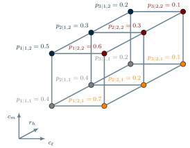
Figure 3: Example of a tensor $\{p_{h|\ell,m}(\bm{\theta})\}_{\ell,m=1,2|h=1,2,3}$ for fixed $\bm{\theta}\in\mathcal{S}_{\bm{\theta}}$.

We model $X_{i}$, $i=1,\dots,N$, as identically distributed random variables ruled by a probability distribution $\mathbb{P}(X_{i};\bm{\gamma})$, depending on a hyperparameter vector $\bm{\gamma}$ whose components take values in a given set $\Gamma$. For notational purposes, we introduce

$$p_{\ell}(\bm{\gamma}):=\mathbb{P}(X_{i}=c_{\ell};\bm{\gamma}).$$ (2)

and, analogously to $\bm{\theta}$, we have the constraint $\bm{\gamma}\in\mathcal{S}_{\Gamma}$ with

$$\mathcal{S}_{\Gamma}:=\Big{\{}\bm{\gamma}\in\Gamma:p_{\ell}(\bm{\gamma})\in[0,1],\sum_{\ell=1}^{C}p_{\ell}(\bm{\gamma})=1\Big{\}}.$$

We assume that $p_{h|\ell,m}$ and $p_{\ell}$ are continuous functions, and that each node knows $p_{h|\ell,m},p_{\ell}$ and the scores received from its in-neighbors and given to its out-neighbors in $G_{S}$.

Notice that the least structured case for the model above is given by the categorical model in which the vector of parameters and the vector of hyperparameters are given by the corresponding probability masses. That is, $\bm{\theta}$ and $\bm{\gamma}$ have respectively $R+2C$ and $C$ components. We point out that the categorical model, being so unstructured, is the most flexible one. Clearly, this flexibility is paid by a much higher number of parameters, which quickly degenerates in over-fitting. Therefore, in practical applications one usually exploits domain-specific knowledge to identify a suitable parametrization in terms of the most relevant parameters and hyperparameters. Some examples are discussed in the next subsection, while the problem of jointly estimating the parameter-hyperparameter $(\bm{\theta},\bm{\gamma})$ will be addressed in the next section as a building block of the (distributed) learning scheme.

II-C Examples of application scenarios

II-C1 Binary-state learning for anomaly detection

We consider a network in which each node $i$ tests neighboring nodes $j$ with a binary outcome indicating if the tested node is deemed faulty (i.e., its state is $x_{j}=1$) or not (i.e., $x_{j}=0$). Since each node performing the evaluation can be itself faulty, its outcome is not always reliable; also, no node knows whether it itself is faulty or not. We consider a probabilistic extension of the well-known Preparata model [24]. Specifically, we assume that the evaluation outcome is determined as follows: if node $i$ is working properly, then it will return the true status of the evaluated node $j$ (i.e., $y_{ij}=1$ if node $j$ is faulty and $y_{ij}=0$ if it is working properly); conversely, if node $i$ is faulty, the outcome is uniformly random. Formally:

$$\begin{split}p_{h|\ell,m}&=(1-c_{\ell})\Big{[}(1-c_{m})(1-r_{h})+c_{m}r_{h}\Big{]}+\frac{1}{2}c_{\ell},\\ p_{\ell}(\gamma)&=\gamma^{c_{\ell}}(1-\gamma)^{1-c_{\ell}},\qquad\gamma\in[0,1],\end{split}$$ (3)

with $R=2$ $(r_{1}=0,r_{2}=1)$ and $C=2$ $(c_{1}=0,c_{2}=1)$. In this first scenario, we assume for simplicity that the distribution of evaluation results is known, so the only unknown is the hyperparameter $\gamma$, which is the a priori probability that a node is faulty. We refer to this model as anomaly-detection model.

II-C2 Social ranking

Another relevant scenario is user profiling in social networks. That is, in social relationships, people naturally tend to aggregate, tacitly or explicitly, into groups based on some affinity.

For example, consider an online forum on a dedicated subject, wherein each member can express her/his preferences by assigning to posts of other members/colleagues a score from $1$ to $R$ indicating an increasing level of appreciation for that post. In order to model the distribution of scores, we consider distance-based ranking distributions, [25], [26], in which (ranking) probabilities decrease as far as the distance from a reference (ranking) probability increases. To fit our needs, we propose for the distribution of scores the following slight variation of the so-called Mallow’s $\phi$-model (see [27]):

$$p_{h|\ell,m}(\theta)=\frac{1}{\psi_{\ell,m}(\theta)}e^{-\big{(}\frac{(r_{R}-r_{h})/r_{R}-d(c_{\ell},c_{m})/c_{C}}{\theta}\big{)}^{2}},$$ (4)

where $r_{h}=h$ ($h=1,\dots,R$), $c_{\ell}=\ell$ ($\ell=1,\dots,C$), $\theta\in\mathbb{R}_{>0}$ is a dispersion parameter, $\psi_{\ell,m}(\theta)$ is a normalizing constant, and $d$ is a semi-distance, i.e., $d\geq 0$ and $d(c_{\ell},c_{m})=0$ iff $c_{\ell}=c_{m}$. Informally, the “farther” a given community $c_{\ell}$ is from another community $c_{m}$, the higher will be the distance $d(c_{\ell},c_{m})$, and thus the lower the score.

In many cases the resulting subgroups reflect some hierarchy in the population. Basic examples could be forums or working teams. Thus, we consider a scenario in which each person belongs to a community reflecting some degree of expertise about a given topic or field. In particular, we have $C$ ordered communities, with $\ell$th community given by $c_{\ell}=\ell$. That is, for example, a person in the community $c_{1}$ is an newbie, while a person in $c_{C}$ is a master. Since climbing in the hierarchy is typically the result of several promotion events, a natural probabilistic model for the communities is a binomial distribution $\mathcal{B}(C-1,\gamma)$, where $\gamma\in[0,1]$ represents the probability of being promoted, i.e.,

$$p_{\ell}(\gamma) =\binom{C-1}{c_{\ell}-1}\gamma^{c_{\ell}-1}(1-\gamma)^{C-1-(c_{\ell}-1)}.$$

We will refer to this second set-up as social-ranking model.

III Interaction-based distributed learning

In this section we describe the proposed distributed learning scheme. Without loss of generality, we concentrate on a set-up in which a node wants to self-classify. The same scheme also applies to a scenario in which a node wants to classify its neighbors, provided it knows their given and received scores. Notice that, in many actual contexts, as, e.g., in social network platforms, this information is readily available.

The section is structured as follows. First, we derive a local Bayesian classifier provided that an estimation of parameter-hyperparameter $(\bm{\theta},\bm{\gamma})$ is available. Then, based on a combination of plain ML and Empirical Bayes estimation approaches, we derive a joint parameter-hyperparameter estimator. Finally, we propose two suitable relaxations of the Score Bayesian Network which lead to distributed estimators, based on proper distributed optimization algorithms.

III-A Bayesian classifiers (given parameter-hyperparameter)

Each node can self-classify (i.e., learn its state) if an estimate $(\bm{\hat{\theta}},\bm{\hat{\gamma}})$ of parameter-hyperparameter $(\bm{\theta},\bm{\gamma})$ is available. Before discussing in details how this estimate can be obtained in a distributed way, we develop a decentralized MAP self-classifier which uses only single-hop information, i.e., the scores it gives to and receives from neighbors.

Formally, let $\bm{y}_{N_{i}}$ be the vector of (observed) scores that agent $i$ obtains by in-neighbors and provides to out-neighbors, i.e., the stack vector of $y_{ji}$ with $(j,i)\in E_{S}$ and $y_{ij}$ with $(i,j)\in E_{S}$. Consistently, let ${\bm{Y}\!}_{N_{i}}$ be the corresponding random vector, then for each agent $i=1,\dots,N$, we define

$$u_{i}(c_{\ell}):=\mathbb{P}(X_{i}=c_{\ell}|{\bm{Y}\!}_{N_{i}}=\bm{y}_{N_{i}};\bm{\hat{\gamma}},\bm{\hat{\theta}}),\quad\ell=1,\dots,C.$$

The soft classifier of $i$ is the probability vector $\bm{u}_{i}:=(u_{i}(c_{1}),\dots,u_{i}(c_{C}))$ (whose components are nonnegative and sum to $1$). In Fig. 4 we depict a pie-chart representation of an example vector $\bm{u}_{i}$.

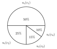
Figure 4: Example of outcome of the soft classifier of an agent $i$, for $C=4$: $\bm{u}_{i}=(0.5,0.25,0.15,0.1)$.

From the soft classifier we can define the classical Maximum A-Posteriori probability (MAP) classifier as the argument corresponding to the maximum component of $u_{i}$, i.e.,

$$\hat{x}_{i}:=\operatorname*{argmax}_{c_{\ell}\in\mathcal{C}}u_{i}(c_{\ell}).$$

The main result here is to show how to efficiently compute the soft and MAP classifiers. First, we define

$$N_{i}^{\leftrightarrow} :=\{j:(j,i)\in E_{S},(i,j)\in E_{S}\},$$

$$N_{i}^{\leftarrow} :=\{j:(j,i)\in E_{S},(i,j)\notin E_{S}\},$$

$$N_{i}^{\rightarrow} :=\{j:(i,j)\in E_{S},(j,i)\notin E_{S}\},$$

and for each $h,k=1,\dots,R$ we introduce the quantities:

$$n_{i}^{\leftrightarrow}(h,k) :=|\{j\in N_{i}^{\leftrightarrow}:y_{ij}=r_{h},y_{ji}=r_{k}\}|,$$

$$n_{i}^{\leftarrow}(h) :=|\{j\in N_{i}^{\leftarrow}:y_{ji}=r_{h}\}|,$$

$$n_{i}^{\rightarrow}(h) :=|\{j\in N_{i}^{\rightarrow}:y_{ij}=r_{h}\}|.$$

Theorem III.1.

Let $i\in\{1,\dots,N\}$ be an agent of the score graph. Then, the components of the vector $u_{i}$ are given by

$$u_{i}(c_{\ell})=\frac{v_{i}(c_{\ell})}{Z_{i}}$$

where $Z_{i}=\sum_{\ell=1}^{C}v_{i}(c_{\ell})$ is a normalizing constant, and $v_{i}(c_{\ell})=p_{\ell}(\bm{\hat{\gamma}})\pi_{i}^{\leftrightarrow}(c_{\ell})\pi_{i}^{\leftarrow}(c_{\ell})\pi_{i}^{\rightarrow}(c_{\ell})$ with

$$\pi_{i}^{\leftrightarrow}(c_{\ell}) =\prod_{h,k=1}^{C}\Big{(}\sum_{m=1}^{C}p_{k|m,\ell}(\bm{\hat{\theta}})p_{h|\ell,m}(\bm{\hat{\theta}})p_{m}(\bm{\hat{\gamma}})\Big{)}^{n_{i}^{\leftrightarrow}(h,k)},$$

$$\pi_{i}^{\leftarrow}(c_{\ell}) =\prod_{h=1}^{R}\Big{(}\sum_{m=1}^{C}p_{h|m,\ell}(\bm{\hat{\theta}})p_{m}(\bm{\hat{\gamma}})\Big{)}^{n_{i}^{\leftarrow}(h)},$$

$$\pi_{i}^{\rightarrow}(c_{\ell}) =\prod_{h=1}^{R}\Big{(}\sum_{m=1}^{C}p_{h|\ell,m}(\bm{\hat{\theta}})p_{m}(\bm{\hat{\gamma}})\Big{)}^{n_{i}^{\rightarrow}(h)}.$$

The proof is given in Appendix -B.

Corollary III.2.

If the score graph is undirected, then we have

$$v_{i}(c_{\ell})=p_{\ell}(\bm{\hat{\gamma}})\pi_{i}^{\leftrightarrow}(c_{\ell}).$$

III-B Joint Parameter-Hyperparameter ML estimation (JPH-ML)

Classification requires that at each node an estimate $(\bm{\hat{\theta}},\bm{\hat{\gamma}})$ of parameter-hyperparameter $(\bm{\theta},\bm{\gamma})$ is available.

On this regard, a few remarks about $\bm{\theta}$ and $\bm{\gamma}$ are now in order. Depending on both the application and the network context, these parameters may be known, or (partially) unknown to the nodes. If both of them are known, we are in a pure Bayesian set-up in which, as just shown, each node can independently self-classify with no need of cooperation. The case of unknown $\bm{\theta}$ (and known $\bm{\gamma}$) falls into a Maximum-Likelihood framework, while the case of unknown $\bm{\gamma}$ (and known $\bm{\theta}$) can be addressed by an Empirical Bayes approach. In this paper we consider a general scenario in which both of them can be unknown. Our goal is then to compute, in a distributed way, an estimate of parameter-hyperparameter $(\bm{\theta},\bm{\gamma})$ and use it for the classification at each node.

In the following we show how to compute it in a distributed way by following a mixed Empirical Bayes and Maximum Likelihood approach. We define the Joint Parameter-Hyperparameter Maximum Likelihood (JPH-ML) estimator as

$$(\bm{\hat{\theta}}_{\text{\tiny ML}},\bm{\hat{\gamma}}_{\text{\tiny ML}}):=\operatorname*{argmax}_{(\bm{\theta},\bm{\gamma})\in\mathcal{S}_{\Theta}\times\mathcal{S}_{\Gamma}}L({\bm{y}\!}_{E_{S}};\bm{\theta},\bm{\gamma})$$ (5)

where ${\bm{y}\!}_{E_{S}}$ is the vector of all scores $y_{ji},(j,i)\in E_{S}$, and

$$L({\bm{y}\!}_{E_{S}};\bm{\theta},\bm{\gamma})=\mathbb{P}({\bm{Y}\!}_{E_{S}}={\bm{y}\!}_{E_{S}}\,;\,\bm{\theta},\bm{\gamma})$$ (6)

is the likelihood function.

Notice that, while $\bm{\theta}$ is directly linked to the observables ${\bm{y}\!}_{E_{S}}$, the hyperparameter $\bm{\gamma}$ is related to the unobservable states. While one could readily obtain the likelihood function for the sole estimation of $\bm{\theta}$ from the distribution of scores, the presence of $\bm{\gamma}$ requires to marginalize over all unobservable state (random) variables. Thus, by using the law of total probability

$$\begin{split}&L({\bm{y}\!}_{E_{S}};\bm{\theta},\bm{\gamma})=\\ &\hskip 5.0pt\sum_{\ell_{1}=1}^{C}\!\cdots\!\sum_{\ell_{N}=1}^{C}\!\mathbb{P}({\bm{Y}\!}_{E_{S}}\!=\!{\bm{y}\!}_{E_{S}},X_{1}\!=\!c_{\ell_{1}},\dots,X_{N}\!=\!c_{\ell_{N}}).\end{split}$$ (7)

Indicating with $N^{I}_{i}$ the set of in-neighbors of agent $i$ in the score graph (we are assuming that it is non-empty), the probability in (7) can be written as the product of the conditional probability of scores, i.e.,

$$\mathbb{P}({\bm{Y}\!}_{E_{S}}={\bm{y}\!}_{E_{S}}\,|\, X_{1}=c_{\ell_{1}},\dots,X_{N}=c_{\ell_{N}})=$$

$$\prod_{i=1}^{N}\prod_{j\in N^{I}_{i}}\mathbb{P}(Y_{ji}=y_{ji}|X_{j}=c_{\ell_{j}},X_{i}=c_{\ell_{i}})$$

multiplied by the prior probability of states, i.e.,

$$\mathbb{P}(X_{1}=c_{\ell_{1}},\dots,X_{N}=c_{\ell_{N}})=\prod_{i=1}^{N}\mathbb{P}(X_{i}=c_{\ell_{i}}).$$

Thus, the likelihood function turns out to be

$$L({\bm{y}\!}_{E_{S}};\bm{\theta},\bm{\gamma})\!=\!\sum_{\ell_{1}=1}^{C}\!\cdots\!\sum_{\ell_{N}=1}^{C}\prod_{i=1}^{N}p_{\ell_{i}}(\bm{\gamma})\prod_{j\in N^{I}_{i}}p_{h_{ji}\,|\,\ell_{i},\ell_{j}}(\bm{\theta})$$

where $h_{ji}$ is the index of the score element $r_{h_{ji}}\in\mathcal{R}=\{r_{1},\ldots,r_{R}\}$ associated to the score $y_{ji}$, i.e., $y_{ji}=r_{h_{ji}}$.

III-C Distributed JPH Node-based Relaxed estimation (JPH-NR)

From the equations above it is apparent that the likelihood function couples the information at all nodes, so problem (5) is not amenable to distributed solution. To make it distributable, we propose a relaxation approach: in particular, we seek for a minimal relaxation in terms of dependencies of the joint probabilities that results in a separable structure of the likelihood function. To this aim we introduce, instead of $L({\bm{y}\!}_{E_{S}};\bm{\theta},\bm{\gamma})$, a Node-based Relaxed (NR) likelihood $L_{NR}({\bm{y}\!}_{E_{S}};\bm{\theta},\bm{\gamma})$. Let $\bm{y}_{N_{i}^{I}}$ be the vector of (observed) scores that agent $i$ obtains by in-neighbors and ${\bm{Y}\!}_{N_{i}^{I}}$ the corresponding random vector. Then,

$$L_{NR}({\bm{y}\!}_{E_{S}};\bm{\theta},\bm{\gamma}):=\prod_{i=1}^{N}\mathbb{P}({\bm{Y}\!}_{N_{i}^{I}}={\bm{y}\!}_{N_{i}^{I}}\,;\,\bm{\theta},\bm{\gamma}).$$ (8)

This relaxation can be interpreted as follows. We pretend that each node has a virtual state, independent from its true state, every time it evaluates another node. Thus, in the Score Bayesian Network, besides the state variables $X_{i}$, $i=1,\dots,N$, there will be additional variables $X_{i}^{\rightarrow j}$ for each $j$ with $(i,j)\in E_{S}$. To clarify this model, Figs. 5-6 depict the node-based relaxed graph and the corresponding graphical model for the same example given in Figs. 1-2.

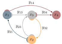
Figure 5: Node-based relaxation of the score graph in Fig. 1, with virtual nodes indicating the virtual states of each node.

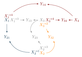
Figure 6: Node-based relaxation of the score Bayesian network of Fig. 5.

Since ${\bm{Y}\!}_{N_{i}^{I}}$, $i=1,\dots,N$, are not independent, then clearly $L\neq L_{NR}$. However, as it will appear from numerical performance assessment, reported in the Section IV, this choice yields reasonably small estimation errors.

Using this virtual independence between ${\bm{Y}\!}_{N_{i}^{I}}$, with $i=1,\dots,N$, we define the JPH-NR estimator as

$$(\bm{\hat{\theta}}_{\text{\tiny NR}},\bm{\hat{\gamma}}_{\text{\tiny NR}}):=\operatorname*{argmax}_{(\bm{\theta},\bm{\gamma})\in\mathcal{S}_{\Theta}\times\mathcal{S}_{\Gamma}}L_{NR}({\bm{y}\!}_{E_{S}};\bm{\theta},\bm{\gamma}).$$ (9)

The next result characterizes the structure of JPH-NR (9).

Proposition III.3.

The JPH-NR estimator based on the node-based relaxation of the score Bayesian network is given by

$$(\bm{\hat{\theta}}_{\text{\tiny NR}},\bm{\hat{\gamma}}_{\text{\tiny NR}})=\operatorname*{argmax}_{(\bm{\theta},\bm{\gamma})\in\mathcal{S}_{\Theta}\times\mathcal{S}_{\Gamma}}\sum_{i=1}^{N}g(\bm{\theta},\bm{\gamma};\bm{n}_{i})$$ (10)

with $\bm{n}_{i}\!=\![n_{i}^{(1)}\cdots n_{i}^{(R)}]^{\top}$, $n_{i}^{(h)}\!:=\!|\{j\in N^{I}_{i}:y_{ji}=r_{h}\}|$, and

$$g(\bm{\theta},\bm{\gamma};\bm{n}_{i}) =$$

$$\log\Big{(}\sum_{\ell=1}^{C} p_{\ell}(\bm{\gamma})\prod_{h=1}^{R}\Big{(}\sum_{m=1}^{C}p_{h\,|\,m,\ell}(\bm{\theta})p_{m}(\bm{\gamma})\Big{)}^{n_{i}^{(h)}}\Big{)}.$$ (11)

The proof is given in Appendix -C.

Proposition III.3 ensures that the JPH-NR estimator can be computed by solving an optimization problem that has a separable cost (i.e., the sum of $N$ local costs). Available distributed optimization algorithms for asynchronous networks can be adopted to this aim, e.g. [28], [29], [30].

III-D Distributed JPH Fully-Relaxed estimation (JPH-FR)

Although JPH-NR estimator is a viable solution for which we will report simulation results later in the paper, we consider a stronger relaxation, which gives rise to a more convenient distributed algorithm consisting of a linear (consensus-like) averaging process and a purely local optimization step.

Thus, we introduce the Fully Relaxed (FR) likelihood:

$$L_{FR}({\bm{y}\!}_{E_{S}};\bm{\theta},\bm{\gamma}):=\prod_{(i,j)\in E_{S}}\mathbb{P}(Y_{ij}=y_{ij}\,;\,\bm{\theta},\bm{\gamma})$$ (12)

where all dependencies among the variables $Y_{ij},(i,j)\in E_{S}$ are neglected. Accordingly, the JPH-FR estimator is given by

$$(\bm{\hat{\theta}}_{\text{\tiny FR}},\bm{\hat{\gamma}}_{\text{\tiny FR}}):=\operatorname*{argmax}_{(\bm{\theta},\bm{\gamma})\in\mathcal{S}_{\Theta}\times\mathcal{S}_{\Gamma}}L_{FR}({\bm{y}\!}_{E_{S}};\bm{\theta},\bm{\gamma}).$$ (13)

The following proposition exposes the structure of (13).

Proposition III.4.

The JPH-FR estimator based on the full relaxation of the score Bayesian network is given by

$$(\bm{\hat{\theta}}_{\text{\tiny FR}},\bm{\hat{\gamma}}_{\text{\tiny FR}})=\operatorname*{argmin}_{(\bm{\theta},\bm{\gamma})\in\mathcal{S}_{\Theta}\times\mathcal{S}_{\Gamma}}\bm{\phi}^{\top}\bm{g}(\bm{\theta},\bm{\gamma})$$ (14)

where $\bm{g}:=(g_{(1)},\dots,g_{(R)}),\quad\bm{\phi}:=(\phi^{(1)},\dots,\phi^{(R)}),$ and

$$g_{(h)}(\bm{\theta},\bm{\gamma}) :=-\log\Big{(}\sum_{\ell,m=1}^{C}p_{h|\ell,m}(\bm{\theta})p_{\ell}(\bm{\gamma})p_{m}(\bm{\gamma})\Big{)},$$

$$\phi^{(h)} :=\sum_{i=1}^{N}\frac{n_{i}^{(h)}}{n},\quad h=1,\dots,R$$

The proof is given in Appendix -D.

In order to solve the optimization problem (14) in a distributed way, each agent in the network needs to know the vector $\bm{\phi}$. A naive approach is to first run a consensus algorithm to obtain approximated local “copies” of $\bm{\phi}$; then, (14) can be solved by applying a standard (centralized) optimization method, e.g. the projected gradient method. However, in this approach one needs to wait for the consensus algorithm to converge (up to the required accuracy), then to start another iterative (local) procedure to finally obtain the solution. We propose here a different approach, where only a single iterative (distributed) procedure is run. The idea is to combine one step of consensus with one step of gradient in order to build a sequence which converges to an optimal solution.

Let $n_{i}$ be the number of incoming edges of agent $i$ into the score graph $G_{S}$, i.e., $n_{i}=|N_{i}^{I}|$. For each $t\in\mathbb{Z}_{\geq 0}$, agent $i$ stores in memory two local states $\bm{\xi}_{i}(t)=(\xi_{i}^{(1)}(t),\dots,\xi_{i}^{(R)}(t))$ and $\eta_{i}(t)$, an estimate $\bm{\phi}_{i}(t)$ of $\bm{\phi}$, and an estimate $(\bm{\hat{\theta}}_{i}(t),\bm{\hat{\gamma}}_{i}(t))$ of $(\bm{\hat{\theta}},\bm{\hat{\gamma}})$.

By following the push-sum consensus algorithm to compute averages in directed graphs [31], we provide the following distributed algorithm to compute $\bm{\phi}$. By denoting $d_{j}(t)=|N_{{\texttt{cmm}},i}^{O}(t)|$ the out-degree of node $j$ at time $t$ in the communication graph $G_{\texttt{cmm}}(t)$, node $i$ implements

$$\begin{split}\xi_{i}^{(h)}(t+1)&=\sum_{j\in N_{i}^{{\texttt{cmm}},I}(t)}\frac{\xi_{j}^{(h)}(t)}{d_{j}(t)}\\ \eta_{i}(t+1)&=\sum_{j\in N_{i}^{{\texttt{cmm}},I}(t)}\frac{\eta_{j}(t)}{d_{j}(t)}\\ \phi_{i}^{(h)}(t+1)&=\frac{\xi_{i}^{(h)}(t+1)}{\eta_{i}(t+1)}\\ \end{split}$$ (15)

with $\xi_{i}^{(h)}(0)=n_{i}^{(h)}$ and $\eta_{i}(0)=n_{i}$.

Then, each node can use its current estimate $\phi_{i}^{(h)}(t)$ to implement a gradient step on the estimated cost function $\bm{\phi}_{i}(t)^{\top}\bm{g}$. That is, let $(\bm{\hat{\theta}}_{i,0},\bm{\hat{\gamma}}_{i,0})\in\mathcal{S}_{\bm{\theta}}\times\mathcal{S}_{\bm{\gamma}}$ be a starting point for the distributed estimation algorithm, $\alpha>0$ a suitable step-size, then $(\bm{\hat{\theta}}_{i}(0),\bm{\hat{\gamma}}_{i}(0))=(\bm{\hat{\theta}}_{i,0},\bm{\hat{\gamma}}_{i,0})$ and

$$\begin{split}(\bm{\hat{\theta}}_{i}(t+1),\bm{\hat{\gamma}}_{i}(t+1))&=\\ \Big{[}(\bm{\hat{\theta}}_{i}(t),\bm{\hat{\gamma}}_{i}(t)&)-\alpha\bm{\phi}_{i}(t)^{\top}\nabla\bm{g}(\bm{\hat{\theta}}_{i}(t),\bm{\hat{\gamma}}_{i}(t))\Big{]}^{+},\end{split}$$ (16)

with $[\cdot]^{+}$ the (Euclidean) projection operator onto the feasible set $\mathcal{S}_{\Theta}\times\mathcal{S}_{\Gamma}$.

The following technical assumption is needed to ensure that this last is well defined.

Assumption III.5.

The given sets $\Theta$ and $\Gamma$ are both subsets of finite-dimensional real-vector spaces, and the product set $\mathcal{S}_{\Theta}\times\mathcal{S}_{\Gamma}$ is compact and convex.

The convergence properties of the distributed algorithm defined by (15)-(16) are given in the following theorem.

Theorem III.6.

Let Assumptions II.1 and III.5 hold. Suppose that $\bm{g}$ is differentiable, and that $\nabla\bm{g}$ is bounded and Lipschitz continuous, with constant $L>0$, over the feasible set $\mathcal{S}_{\Theta}\times\mathcal{S}_{\Gamma}$. Let $0<\alpha<\frac{2}{L}$. Then, any limit point of the sequence $\{(\bm{\hat{\theta}}_{i}(t),\bm{\hat{\gamma}}_{i}(t))\}_{t\in\mathbb{N}}$ generated by (15)-(16) is a stationary point of the objective function $\bm{\phi}^{\top}\bm{g}$ over the feasible set $\mathcal{S}_{\Theta}\times\mathcal{S}_{\Gamma}$.

The proof is given in Appendix -E.

IV Application of the framework

In this section we provide numerical results for two meaningful case studies, using the anomaly-detection and the social-ranking models described in Section II-C. Beforehand, we analyze a special binary/binary case for which the JPH-FR estimator can be computed in closed form.

IV-A Distributed learning for anomaly detection: binary scores and binary states

For the anomaly-detection model described in Section II-C, $C=R=2$ is a very special case where a closed form solution for the JPH-FR optimization problem can be found. Using Lemma .4 we compute the fully relaxed likelihood as

$$L_{FR}(\gamma)=\Big{[}\frac{1}{2}\gamma+\gamma(1-\gamma)\Big{]}^{n^{(2)}}\Big{[}\frac{1}{2}\gamma+(1-\gamma)^{2}\Big{]}^{n^{(1)}}$$

whose derivative is

$$L_{FR}^{\prime}(\gamma)=n\Big{[}\frac{1}{2}\gamma+\gamma(1-\gamma)\Big{]}^{n^{(2)}-1}\Big{[}\frac{1}{2}\gamma+(1-\gamma)^{2}\Big{]}^{n^{(1)}-1}h_{0}(\gamma)$$

with

$$h_{0}(\gamma)=\phi^{(2)}\Big{(}\frac{3}{2}-2\gamma\Big{)}\Big{(}\frac{1}{2}\gamma+(1-\gamma)^{2}\Big{)}\\ -\phi^{(1)}\Big{(}\frac{3}{2}-2\gamma\Big{)}\Big{(}\frac{1}{2}\gamma+\gamma(1-\gamma)\Big{)}.$$

The first two factors have roots that give a zero cost function, thus optimizers are obtained by studying the sign of $h_{0}(\gamma)$. Its roots are $\gamma_{0}=\frac{3}{4}$ and $\gamma_{1,2}=\frac{1}{4}(3\pm\sqrt{9-16\phi^{(2)}})$, and straightforward computations show that for $\phi^{(2)}\leq\frac{9}{16}$ both $\gamma_{1}$ and $\gamma_{2}$ are (real) local maximizers. However, $\gamma_{2}=\frac{1}{4}(3+\sqrt{9-16\phi^{(2)}})\geq 1$. Thus, we conclude that

$$\hat{\gamma}_{\text{\tiny FR}}=\begin{cases}\frac{3}{4}&\text{if}\;\phi^{(2)}\geq\frac{9}{16}\\[5.16663pt] \frac{1}{4}(3-\sqrt{9-16\phi^{(2)}})&\text{otherwise}.\end{cases}$$

With the expression of $\hat{\gamma}_{\text{\tiny FR}}$ in hand, we are able to compute the soft and the MAP classifiers according to Theorem III.1, hence only a consensus on $\bm{\phi}$ is needed.

Besides this special (binary-binary) case, in general it is not possible to find a closed form, hence the proposed distributed estimators are needed in practice. Indeed, in the next example we show that, as soon as we remove the hypothesis that scores are binary, the cost function becomes analytically intractable, so that numerical optimization algorithms, as the ones we are proposing in this paper, are unavoidable.

IV-B Distributed learning for anomaly detection: $R$-ary scores and binary states

We consider an extension of the previous scenario by allowing scores to assume multiple values. We basically relax the fact that a normally working node gives the exact state of the tested node in a deterministic way. We assume that the $R$ possible scores are given according to some probability, depending e.g. on the reliability of the test or expressing the level of trust about the tested node. For the sake of clarity we just consider a linear trend. Formally, we let

$$R \geq 2,\quad\,\,\,\,\,r_{h}=h-1,\quad h=1,\dots,R,$$

$$C =2,\quad\,\,\,\,\,c_{1}=0,\quad\,\,c_{2}=1,$$

and consider the following probabilistic model:

$$p_{h|\ell,m} =\frac{2}{R}(1-c_{\ell})\Big{[}(1-c_{m})\Big{(}1-\frac{r_{h}}{r_{R}}\Big{)}+c_{m}\frac{r_{h}}{r_{R}}\Big{]}+\frac{c_{\ell}}{R},$$

$$p_{\ell}(\gamma) =\gamma^{c_{\ell}}(1-\gamma)^{1-c_{\ell}},\qquad\gamma\in[0,1].$$

Notice that this model, hereafter referred to as the reliability model, boils down to the Preparata model [24] for the case of binary score ($R=2$, see Sec. II-C1). Clearly, Lemma .4 with the expression above for $p_{h|\ell,m}$ does not have a closed form solution, hence we show the solution by numerical analysis.

We have performed Monte Carlo simulations, with $1000$ trials for each point, for a score graph with $N=300$ agents according to the probabilistic model above, for $R=5$ and $\gamma=\frac{3}{10}$. As for the score graph, we considered a sequence of scenarios by starting from a directed cyclic configuration and then, progressively, adding edges up to the complete graph.

We considered the reliability model to compute both the JPH-NR and the JPH-FR estimator of the hyperparameter, which in this case is $\gamma=\frac{3}{10}$; then we have used these estimators to perform the classification. Results of these simulations are shown in Fig. 7, where the Root Mean Square Error (RMSE) of the estimates of $\gamma$ is reported for the two proposed estimators.

Figure 7: RMSE of the estimates of $\gamma$ as a function of the number of edges $n$.

Remarkably, both estimators are able to provide a very good estimate, which improves as $n$ increases (as one might expect); moreover, the JPH-FR is very close to the JPH-NR. The impact of such estimates of the hyperparameter onto the misclassification rate is reported in Fig. 8.

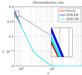
Figure 8: Misclassification rate as function of the number of edges $n$ increasing from $N$ (cyclic graph) to $N^{2}-N$ (complete graph), with $N=300$, $\gamma=\frac{3}{10}$ and $R=5$.

As a benchmark, the curve corresponding also to the “oracle” classifier that uses the true value of $\gamma$ is reported. Results for this case are rather impressive, since both the proposed estimator are practically attaining the performance of the “oracle” classifier. This indicates that the proposed relaxations are able to retain the salient aspects of the statistical relationship among the variables, yielding results as good as the true graphical model.

IV-C Distributed learning for social ranking

In this Section we report results for the social-ranking model described in Section II-C with $C=3$, $R=3$ and $N=300$. We use as semi-distance in (4) $d(c_{\ell},c_{m})=|c_{\ell}-c_{m}|=|\ell-m|$, and as true parameter-hyperparameter $\theta=\frac{1}{2}$ and $\gamma=\frac{3}{10}$.

Monte Carlo simulations have been run to test both JPH-NR and JPH-FR, with $1000$ trials for each point. Compared to the previous case, both parameter and hyperparameter are (jointly) estimated. Figs. 9-10 report the RMSE for $\theta$ and $\gamma$, respectively, as a function of the number of edges. It is worth noting that both the estimation errors decrease as the number of edges increases (more data are available) and the “less relaxed” JPH-NR estimator slightly outperforms the JPH-FR.

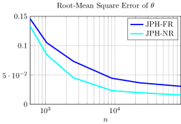
Figure 9: RMSE of the estimates of $\theta$ as a function of the number of edges.

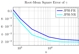
Figure 10: RMSE of the estimates of $\gamma$ as a function of the number of edges.

The impact of estimation errors on the learning performance is shown in Fig. 11: the curves clearly show that, compared to the reliability model, the inferential relationship between scores and states is “weaker” hence more data are needed for a good learning. Nonetheless, the proposed estimators are still very close to the performance of the benchmark (“oracle”).

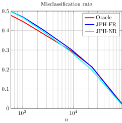
Figure 11: Misclassification rate as function of the number of edges $n$ increasing from $N$ (cyclic graph) to $N^{2}-N$ (complete graph), with $N=300$, $\gamma=\frac{3}{10}$, $\theta=\frac{1}{2}$, $C=3$ and $R=3$.

Finally, we report an additional case to highlight the usefulness of the soft classifier. We considered a network of $N=10$ agents, whose score graph $G_{S}$ is shown in Fig. 12. We drew the states and scores in the given score graph according to the previous distributions, and then used the social-ranking model to solve the learning problem as before, by means of the JPH-FR estimator.

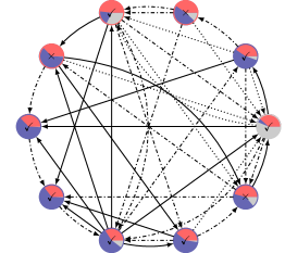
Figure 12: Soft classifier representation of a particular score graph.

The contour of a node has a color which indicates the true state of the node. Inside the node we have represented the outcome of the soft classification, i.e., the output of the local self-classifier, as a pie-chart. The colors used are: red for state $1$, blue for state $2$, gray for state $3$. Moreover, each edge is depicted by a different pattern based on its evaluation result $r_{h}$: solid lines are related to scores equal to $3$, dash dot lines are related to scores equal to $2$, while dotted lines are related to scores equal to $1$. We assigned to each node a symbol $\checkmark$ or $\times$ indicating if the MAP classifier correctly decided for the true state or not. We show a realization with three misclassification errors; remarkably, all of them correspond to a lower confidence level given by the soft classifier, which is an important indicator of the lack of enough information to reasonably trust the decision. It can be observed that the edge patterns concur to determine the decision. Indeed, the only gray-state node is correctly classified thanks to the predominant number of dotted edges insisting on it, and similarly for the blue-state nodes which mostly have solid incoming edges. When a mix of scores are available, clearly there is more uncertainty and the learning may fail, as for two of the red-state nodes.

As a final remark, we point out that in some scenarios symmetries may arise in the model, thus creating ambiguities in the labeling of the communities. Specifically, for this scenario, it can be proven that the relaxed likelihoods $L_{NR}$ and $L_{FR}$ take on the same value when $\gamma$ is replaced by $1-\gamma$, e.g., $L_{NR}({\bm{y}\!}_{E_{S}};\bm{\theta},\bm{\gamma})=L_{NR}({\bm{y}\!}_{E_{S}};\bm{\theta},1-\bm{\gamma})$. Thus the hyperparameter estimate is not unique in this case. However, this has just the effect of swapping the label of communities $c_{1}$ and $c_{3}$. Notice that, in the node-based relaxed case, agents reach directly a consensus on the same value, thus circumventing possible inconsistencies in the labeling. For the fully relaxed case agents can easily agree on the same value in a number of steps equal to the diameter.

V Conclusion

In this paper we have proposed a novel probabilistic framework for distributed learning, which is particularly relevant to emerging contexts such as cyber-physical systems and social networks. In the proposed set-up, nodes of a network want to learn their (unknown) state, as typical in classification problems; however, differently from a classical set-up, the information does not come from (noisy) measurements of the state but rather from observations produced by the interaction with other nodes. For this problem we have proposed a hierarchical (Bayesian) framework in which the parameters of the interaction model as well as hyperparameters of the prior distributions may be unknown. Node classification is performed by means of a local Bayesian classifier that uses parameter-hyperparameter estimates, obtained by combining the plain ML with the Empirical Bayes estimation approaches in a joint scheme. The resulting estimator is very general but, unfortunately, not amenable to distributed computation. Therefore, by relying on the conceptual tool of graphical models, we have proposed two approximated ML estimators that exploit proper relaxations of the conditional dependences among the involved random variables. Remarkably, the two approximated likelihood functions do lead to distributed estimation algorithms: specifically, for the node-based relaxed estimator, available distributed optimization algorithms can be used, while for the fully relaxed a faster scheme can be implemented that combines a local descent step with a diffusion (consensus-based) step. To demonstrate the application of the proposed schemes, we have addressed two example scenarios from anomaly detection in cyber-physical networks and user profiling in social networks, for which Monte Carlo simulations are reported. Results show that the proposed distributed learning schemes, although based on relaxations of the exact likelihood function, exhibit performance very close to the ideal classifier that has perfect knowledge of all parameters.

-A Preliminaries on Bayesian Networks

Before proving Theorem III.1, we need to recall some useful definitions and results from graphical model theory. We want to understand when two random variables $Z_{\text{in}}$ and $Z_{\text{fin}}$ in a distribution associated with a Bayesian Network structure $\mathcal{K}$ are conditionally independent given another variable $Z_{g}$. We first introduce a shorthand notation. We write $Z_{i}\rightleftharpoons Z_{i+1}$ meaning that either $Z_{i}\rightarrow Z_{i+1}$, or $Z_{i}\leftarrow Z_{i+1}$, or both hold.

Definition .1.

Given a graphical model $\mathcal{K}$, we say that $Z_{0},\dots,Z_{r}$ form a trail in $\mathcal{K}$ if, for every $i=0,\dots,r-1,$ we have $Z_{i}\rightleftharpoons Z_{i+1}$. If, for every $i=0,\dots,r-1,$ we have that $Z_{i}\rightarrow Z_{i+1}$, then the trail is called a directed path.

Definition .2.

We say that $Z_{d}$ is a descendant of $Z$ in the graph $\mathcal{K}$ if there exists a directed path from $Z$ to $Z_{d}$.

When influence can flow from $Z_{\text{in}}$ to $Z_{\text{fin}}$ via $Z_{g}$, we say that the two-arrow trail $Z_{\text{in}}\rightleftharpoons Z_{g}\rightleftharpoons Z_{\text{fin}}$ is active. For each of the four possible two-arrow trails, we detail the condition under which it is active:

• Causal trail ($Z_{\text{in}}\rightarrow Z_{g}\rightarrow Z_{\text{fin}}$): active if and only if $Z_{g}$ is not observed.

• Evidential trail ($Z_{\text{in}}\leftarrow Z_{g}\leftarrow Z_{\text{fin}}$): active if and only if $Z_{g}$ is not observed.

• Common cause ($Z_{\text{in}}\leftarrow Z_{g}\rightarrow Z_{\text{fin}}$): active if and only if $Z_{g}$ is not observed.

• Common effect ($Z_{\text{in}}\rightarrow Z_{g}\leftarrow Z_{\text{fin}}$): active if and only if either $Z_{g}$ or one of its descendants is observed.

Now, consider the case of a longer trail $Z_{\text{in}}=Z_{0}\rightleftharpoons\cdots\rightleftharpoons Z_{r}=Z_{\text{fin}}$. Intuitively, for influence to flow from $Z_{\text{in}}$ to $Z_{\text{fin}}$, it needs to flow through every single node on the trail. In other words, $Z_{0}$ can influence $Z_{r}$ if for every $i=1,\ldots,r-1$, then $Z_{i-1}\rightleftharpoons Z_{i}\rightleftharpoons Z_{i+1}$ is active.

Obviously, it can happen that there is more than one trail between two nodes; in these cases one node can influence another if and only if there exists a trail along which influence can flow. If there is no active trail between two random variables $Z_{\text{in}}$ and $Z_{\text{fin}}$, given random variable $Z_{g}$, they are said to be d-separated.

-B Proof of Theorem III.1

We are now ready to give the following lemma needed for the proof of Theorem III.1.

Lemma .3.

Let $i,j,k\in\{1,\ldots,N\}$ with $j\neq k$. The following statements hold:

1. if $(i,j),(k,i)\in E_{S}$ then $Y_{ij}$ and $Y_{ki}$ are conditionally independent given $X_{i}$;

2. if $(i,j),(i,k)\in E_{S}$ then $Y_{ij}$ and $Y_{ik}$ are conditionally independent given $X_{i}$;

3. if $(j,i),(k,i)\in E_{S}$ then $Y_{ji}$ and $Y_{ki}$ are conditionally independent given $X_{i}$;

Proof.

We prove only the first statement, the other two can be proven in the same way. Consider a trail $Y_{ij}=Z_{0}\rightleftharpoons\cdots\rightleftharpoons Z_{r}=Y_{ki}$. Denoting by $s$ the number of state random variables traversed along the trail, then the length of the trail (number of arrows) is $r=2s$. This property can be easily visualized in Figure 2. For each $u=0,\dots,s-1$ it results:

$$Z_{2u}\leftarrow Z_{2u+1}\rightarrow Z_{2u+2}$$

with

$$Z_{2u}=Y_{i_{u}j_{u}},\quad Z_{2u+1}=X_{v_{u}},\quad Z_{2u+2}=Y_{i_{u+1}j_{u+1}},$$

where we have that $v_{u}\in\{i_{u},j_{u}\}\cap\{i_{u+1},j_{u+1}\}$, while $(i_{u},j_{u}),(i_{u+1},j_{u+1})\in E_{S}$.

Our objective is to prove that the previous trail is blocked (i.e., not active); this will imply that $Y_{ij},Y_{ki}$ are $d$-separated given $X_{i}$, so that the proof follows, [32]. We observe that if $X_{v_{0}}=X_{i}$, then we have, inside the trail, the common cause $Z_{0}\leftarrow X_{i}\rightarrow Z_{2}$ in which $X_{i}$ is observed; thus the previous common cause is blocked, implying that also the trail is blocked. Next, we prove that block occurs at most for $u=1$. Consider $X_{v_{0}}\neq X_{i}$. In this case, from the assumption $j\neq k$, by contradiction, we find that $s>1$. By truncating the trail at the fourth element, we have:

$$Z_{0}\leftarrow X_{v_{0}}\rightarrow Z_{2}\leftarrow X_{v_{1}}.$$

In the common effect $X_{v_{0}}\rightarrow Z_{2}\leftarrow X_{v_{1}}$, $Z_{2}$ is not observed, and $Z_{2}=Y_{i_{1}j_{1}}$ has no descendant in the graphical model; thus the previous common effect is blocked, implying that also the trail is blocked. ∎

After these preliminaries, we can proceed with the proof of Theorem III.1. For the sake of clarity of notation, we will omit the dependency on $\bm{\theta}$ and $\bm{\gamma}$.

From the Bayes theorem, we know that:

$$u_{i}(c_{\ell})=\frac{v_{i}(c_{\ell})}{\mathbb{P}(\bm{Y}_{N_{i}}=\bm{y}_{N_{i}})},$$

where $v_{i}(c_{\ell}):=\mathbb{P}(\bm{Y}_{N_{i}}=\bm{y}_{N_{i}},X_{i}=c_{\ell})$. Our goal is to prove that $v_{i}(c_{\ell})=p_{\ell}(\bm{\hat{\gamma}})\pi_{i}^{\leftrightarrow}(c_{\ell})\pi_{i}^{\leftarrow}(c_{\ell})\pi_{i}^{\rightarrow}(c_{\ell})$. First of all, from the chain rule we have:

$$v_{i}(c_{\ell}) =\mathbb{P}(X_{i}=c_{\ell})\mathbb{P}(\bm{Y}_{N_{i}}=\bm{y}_{N_{i}}|X_{i}=c_{\ell}),$$ (17)

and from Lemma .3, we know that

$$\mathbb{P}(\bm{Y}_{N_{i}}\!=\!\bm{y}_{N_{i}}|X_{i}\!=\!c_{\ell}) =\mathbb{P}(\bm{Y}_{N_{i}^{\leftrightarrow}}\!=\!\bm{y}_{N_{i}^{\leftrightarrow}}|X_{i}\!=\!c_{\ell})$$

$$\quad\times\mathbb{P}(\bm{Y}_{N_{i}^{\leftarrow}}\!=\!\bm{y}_{N_{i}^{\leftarrow}}|X_{i}\!=\!c_{\ell})$$ (18)

$$\quad\times\mathbb{P}(\bm{Y}_{N_{i}^{\rightarrow}}\!=\!\bm{y}_{N_{i}^{\rightarrow}}|X_{i}\!=\!c_{\ell}).$$

The next step is to study each one of the three factors. Starting from $\mathbb{P}(\bm{Y}_{N_{i}^{\leftrightarrow}}=\bm{y}_{N_{i}^{\leftrightarrow}}|X_{i}=c_{\ell})$, we obtain:

$$\!\!\!\!\!\!\!\mathbb{P}(\bm{Y}_{N_{i}^{\leftrightarrow}}\!\!=\!\!\bm{y}_{N_{i}^{\leftrightarrow}}|X_{i}\!\!=\!\!c_{\ell})$$

$$= \prod_{j\in N_{i}^{\leftrightarrow}}\!\!\mathbb{P}(Y_{ij}\!\!=\!\!y_{ij},Y_{ji}\!\!=\!\!y_{ji}|X_{i}\!\!=\!\!c_{\ell})$$

$$= \prod_{h,k=1}^{R}\!\!\mathbb{P}(Y_{ij_{0}}=r_{h},Y_{j_{0}i}=r_{k}|X_{i}=c_{\ell})^{n^{\leftrightarrow}_{i}(h,k)}$$

$$= \prod_{h,k=1}^{R}\!\!\!\Big{(}\sum_{m=1}^{C}\mathbb{P}(Y_{ij_{0}}\!\!=\!\!r_{h},Y_{j_{0}i}\!\!=\!\!r_{k},X_{j_{0}}\!\!=\!\!c_{m}|X_{i}\!\!=\!\!c_{\ell})\Big{)}^{n^{\leftrightarrow}_{i}(h,k)}$$

$$= \prod_{h,k=1}^{R}\!\!\Big{(}\sum_{m=1}^{C}\mathbb{P}(X_{j_{0}}\!\!=\!\!c_{m})\mathbb{P}(Y_{ij_{0}}\!\!=\!\!r_{h}|X_{i}\!\!=\!\!c_{\ell},X_{j_{0}}\!\!=\!\!c_{m})$$

$$\hskip 45.0pt\times\mathbb{P}(Y_{j_{0}i}\!\!=\!\!r_{k}|X_{j_{0}}\!\!=\!\!c_{m},X_{i}\!\!=\!\!c_{\ell})\Big{)}^{n^{\leftrightarrow}_{i}(h,k)}.$$ (19)

In the first equation we have used again Lemma .3; in the second equation we have used the fact that $Y_{ij},(i,j)\in E_{S}$ are identically distributed, and we have also aggregated the agents in $N_{i}^{\leftrightarrow}$ that receive/give score $r_{h}/r_{k}$ from/to agent $i$; in the third equation we have marginalized with respect to the random variable $X_{j_{0}}$; in the fourth equation we have factorized according to the score Bayesian network.

For the second factor $\mathbb{P}(\bm{Y}_{N_{i}^{\leftarrow}}=\bm{y}_{N_{i}^{\leftarrow}}|X_{i}=c_{\ell})$, we obtain:

$$~{}\mathbb{P}(\bm{Y} {}_{N_{i}^{\leftarrow}}=\bm{y}_{N_{i}^{\leftarrow}}|X_{i}=c_{\ell})$$

$$= \prod_{j\in N_{i}^{\leftarrow}}\mathbb{P}(Y_{ji}=y_{ji}|X_{i}=c_{\ell})$$

$$= \prod_{h=1}^{R}\mathbb{P}(Y_{j_{0}i}=r_{h}|X_{i}=c_{\ell})^{n_{i}^{\leftarrow}(h)}$$

$$= \prod_{h=1}^{R}\Big{(}\sum_{m=1}^{C}\mathbb{P}(Y_{j_{0}i}=r_{h},X_{j_{0}}=c_{m}|X_{i}=c_{\ell})\Big{)}^{n_{i}^{\leftarrow}(h)}$$

$$= \prod_{h=1}^{R}\Big{(}\sum_{m=1}^{C}\mathbb{P}(X_{i}=c_{m})$$

$$\hskip 25.0pt\times\mathbb{P}(Y_{j_{0}i}=r_{h}|X_{j_{0}}=c_{m},X_{i}=c_{\ell})\Big{)}^{n_{i}^{\leftarrow}(h)}.$$ (20)

Here, we point out that, when using Lemma .3 in the first equation, all the random variables $\bm{Y}_{N_{i}^{\leftarrow}}$ are conditionally independent given $X_{i}$. Also, factors in the second equation are aggregated based on the agents in the set $N_{i}^{\leftarrow}$ that give score $r_{h}$ to agent $i$.

Finally, the third factor turns out to be:

$$~{}\mathbb{P}(\bm{Y} {}_{N_{i}^{\rightarrow}}=\bm{y}_{N_{i}^{\rightarrow}}|X_{i}=c_{\ell})$$

$$= \prod_{h=1}^{R}\Big{(}\sum_{c_{m}=1}^{C}\mathbb{P}(X_{i}=c_{m})$$

$$\hskip 25.0pt\times\mathbb{P}(Y_{ij_{0}}=r_{h}|X_{i}=c_{\ell},X_{j_{0}}=c_{m})\Big{)}^{n_{i}^{\rightarrow}(h)}.$$ (21)

Plugging together (-B), (-B), (-B) into (-B), and then into (17), the proof is complete.

-C Proof of Proposition III.3

We omit the dependency on $\bm{\theta}$ and $\bm{\gamma}$ for notational purposes.

Consider a factor $\mathbb{P}({\bm{Y}\!}_{N_{i}^{I}}={\bm{y}\!}_{N_{i}^{I}})$ of the node-based relaxed likelihood, with $i$ an agent in the score graph. Marginalizing with respect to $X_{i}$, we have

$$\mathbb{P}({\bm{Y}\!}_{N_{i}^{I}}={\bm{y}\!}_{N_{i}^{I}})=\sum_{\ell=1}^{C}\mathbb{P}({\bm{Y}\!}_{N_{i}^{I}}={\bm{y}\!}_{N_{i}^{I}},X_{i}=c_{\ell}).$$

Now, applying the chain rule we obtain

$$\mathbb{P}({\bm{Y}\!}_{N_{i}^{I}}={\bm{y}\!}_{N_{i}^{I}})=\sum_{\ell=1}^{C}\mathbb{P}(X_{i}=c_{\ell})\mathbb{P}({\bm{Y}\!}_{N_{i}^{I}}={\bm{y}\!}_{N_{i}^{I}}|X_{i}=c_{\ell}).$$

We are then ready to use Lemma .3, which implies that

$$\mathbb{P}({\bm{Y}\!}_{N_{i}^{I}}={\bm{y}\!}_{N_{i}^{I}})=\sum_{\ell=1}^{C}\mathbb{P}(X_{i}=c_{\ell})\!\prod_{j\in N_{i}^{I}}\!\mathbb{P}(Y_{ji}=y_{ji}|X_{i}=c_{\ell}).$$

Recalling that $Y_{ij},(i,j)\in E_{S}$ are identically distributed, we aggregate all the agents in $N_{i}^{I}$ that give score $r_{h}$ to agent $i$:

$$\mathbb{P}({\bm{Y}\!}_{N_{i}^{I}}\!=\!{\bm{y}\!}_{N_{i}^{I}})\!=\!\sum_{\ell=1}^{C}\mathbb{P}(X_{i}\!=\!c_{\ell})\prod_{h=1}^{R}\mathbb{P}(Y_{j_{0}i}\!=\!r_{h}|X_{i}\!=\!c_{\ell})^{n_{i}^{(h)}},$$

and marginalize with respect to $X_{j_{0}}$, thus obtaining

$$\mathbb{P}({\bm{Y}\!}_{N_{i}^{I}}={\bm{y}\!}_{N_{i}^{I}})=\sum_{\ell=1}^{C}\!\mathbb{P}(X_{i}\!=\!c_{\ell})$$

$$\hskip 50.0pt\times\prod_{h=1}^{R}\!\Big{(}\!\sum_{m=1}^{C}\!\mathbb{P}(Y_{j_{0}i}\!=\!r_{h},X_{j_{0}}\!=\!c_{m}|X_{i}\!=\!c_{\ell})\Big{)}^{n_{i}^{(h)}}.$$

From the structure of the score Bayesian network the following factorization is obtained:

$$\mathbb{P}({\bm{Y}\!}_{N_{i}^{I}}\!=\!{\bm{y}\!}_{N_{i}^{I}})\! =\!\sum_{\ell=1}^{C}\mathbb{P}(X_{i}\!=\!c_{\ell})\!\prod_{h=1}^{R}\!\Big{(}\sum_{m=1}^{C}\mathbb{P}(X_{j_{0}}\!=\!c_{m})$$

$$\hskip 10.0pt\times\mathbb{P}(Y_{j_{0}i}\!=\!r_{h}|X_{j_{0}}\!=\!c_{m},X_{i}\!=\!c_{\ell})\Big{)}^{n_{i}^{(h)}}.$$

Then, the node-based relaxed likelihood $L_{NR}$ is the product over $i=1,\ldots,N$ of the factors above, so that

$$L_{NR}(\bm{\theta},\bm{\gamma})=\prod_{i=1}^{N}\sum_{\ell=1}^{C}p_{\ell}(\bm{\gamma})\prod_{h=1}^{R}\Big{(}\sum_{m=1}^{C}p_{h|m,\ell}(\bm{\theta})p_{m}(\bm{\gamma})\Big{)}^{n_{i}^{(h)}},$$

where we have used the shorthand notation introduced in (2) and (1).

Applying the logarithm to the expression of $L_{NR}(\bm{\theta},\bm{\gamma})$ derived above, it follows immediately that $\log(L_{NR}(\bm{\theta},\bm{\gamma}))=\sum_{i=1}^{N}g(\bm{\theta},\bm{\gamma};\bm{n}_{i}),$ with each $g(\bm{\theta},\bm{\gamma};\bm{n}_{i})$ as in (III.3). Finally, since the logarithm is increasing, the maximum argument is invariant under this transformation, thus concluding the proof.

-D Proof of Proposition III.4

Before proving Proposition III.4 we give a useful lemma:

Lemma .4.

The fully relaxed likelihood can be written as

$$L_{FR}(\bm{\theta},\bm{\gamma})=\prod_{h=1}^{R}\Big{(}\sum_{\ell,m=1}^{C}p_{h|\ell,m}(\bm{\theta})p_{\ell}(\bm{\gamma})p_{m}(\bm{\gamma})\Big{)}^{n^{(h)}},$$

where $n^{(h)}:=|\{(i,j)\in E_{S}:y_{ij}=r_{h}\}|$.

Proof.

In what follows, we omit the dependency on $\bm{\theta}$ and $\bm{\gamma}$. We start focusing our attention on the product $\prod_{(i,j)\in E_{S}}\mathbb{P}(Y_{ij}=y_{ij})$, which gives the fully relaxed likelihood. Recalling that $Y_{ij},(i,j)\in E_{S}$, are identically distributed, and aggregating the edges $(i,j)$ for which $y_{ij}=r_{h}$, we obtain

$$\prod_{(i,j)\in E_{S}}\mathbb{P}(Y_{ij}=y_{ij})=\prod_{h=1}^{R}\mathbb{P}(Y_{i_{0}j_{0}}=r_{h})^{n^{(h)}},$$

with $(i_{0},j_{0})$ being an arbitrary edge in $E_{S}$. Then, marginalizing with respect to $X_{i_{0}}$ and $X_{j_{0}}$, it follows that

$$\prod_{(i,j)\in E_{S}} \mathbb{P}(Y_{ij}=y_{ij})$$

$$= \prod_{h=1}^{R}\Big{(}\sum_{\ell,m=1}^{C}\mathbb{P}(Y_{i_{0}j_{0}}\!=\!r_{h},X_{i_{0}}\!=\!c_{\ell},X_{j_{0}}\!=\!c_{m})\Big{)}^{n^{(h)}}.$$

Finally, exploiting again the structure of the Bayesian network, we have that

$$\prod_{(i,j)\in E_{S}}\!\!\!\mathbb{P}(Y_{ij}\!=\!y_{ij}) \!=\!\prod_{h=1}^{R}\!\Big{(}\!\sum_{\ell,m=1}^{C}\mathbb{P}(X_{i_{0}}\!=\!c_{\ell})\mathbb{P}(X_{j_{0}}\!=\!c_{m})$$

$$\hskip 5.0pt\times\mathbb{P}(Y_{i_{0}j_{0}}\!=\!r_{h}|X_{i_{0}}\!=\!c_{\ell},X_{j_{0}}\!=\!c_{m})\Big{)}^{n^{(h)}},$$

so that the proof follows. ∎

Now we are ready to prove Proposition III.4. Since the logarithm is a monotone transformation, it follows straight that

$$(\bm{\hat{\theta}}_{\text{\tiny FR}},\bm{\hat{\gamma}}_{\text{\tiny FR}}) =\operatorname*{argmin}_{(\bm{\gamma},\bm{\theta})\in\mathcal{S}_{\bm{\gamma}}\times\mathcal{S}_{\bm{\theta}}}-\frac{1}{n}\log(L_{FR}(\bm{\theta},\bm{\gamma})).$$ (22)

Using Lemma .4, we have that:

$$-\frac{1}{n}\log(L_{FR}(\bm{\theta},\bm{\gamma})) =$$

$$-\sum_{h=1}^{R}\frac{n^{(h)}}{n} \log\Big{(}\sum_{\ell,m=1}^{C}p_{h|\ell,m}(\bm{\theta})p_{\ell}(\bm{\gamma})p_{m}(\bm{\gamma})\Big{)},$$ (23)

so that it is easy to show that

$$n^{(h)}=\sum_{i=1}^{N}n_{i}^{(h)}.$$ (24)

Plugging together (22), (-D), and (24), the proof follows.

-E Proof of Theorem III.6

Before proving Theorem III.6, we give two Lemmas.

Lemma .5.

Let Assumption II.1 holds, and consider $i\in\{1,\dots,N\}$. Then there exist $C>0$, $d\in[0,1)$ and $T>0$, such that,

$$\|\bm{\phi}-\bm{\phi}_{i}(t)\|\leq d^{t}C,$$ (25)

for all $t\geq T$.

Proof.

The proof follows the same steps as in [29], details are omitted for the sake of conciseness. ∎

Lemma .6.

Let $A_{t},B_{t},C_{t}$ be three sequences such that $B_{t}$ is nonnegative for all $t$. Assume that

$$A_{t+1}\leq A_{t}-B_{t}+C_{t},$$

and that the series $\sum_{t=0}^{\infty}C_{t}$ converges. Then either $A_{t}\to-\infty$ or else $A_{t}$ converges to a finite value and $\sum_{t=0}^{\infty}B_{t}<\infty$.

Proof.

For the proof see Lemma 1 in [33]. ∎

We now prove Theorem III.6. For notational purposes, we define:

$$z_{i}^{t} :=(\bm{\hat{\theta}}_{i}(t),\bm{\hat{\gamma}}_{i}(t)),$$

$$\quad\overline{z}_{i}^{t} :=[z_{i}^{t}-\alpha\bm{\phi}_{i}(t)^{\top}\nabla\bm{g}(z_{i}^{t})]^{+},$$ (26)

$$g_{\phi}(\bm{\theta},\bm{\gamma}) :=\bm{\phi}^{\top}\bm{g}(\bm{\theta},\bm{\gamma}).$$

Let $\hat{z}_{i}$ be a limit-point of $\{z_{i}^{t}\}_{t\geq 0}$; taking into account that the stepsize is constant, our strategy is to prove that $\hat{z}_{i}$ is a stationary point of $g_{\phi}$ over $\mathcal{S}_{\bm{\theta}}\times\mathcal{S}_{\bm{\gamma}}$ by showing that $\hat{z}_{i}$ is a fixed point of the projected gradient method related to the objective function $g_{\phi}$ and to the feasible set $\mathcal{S}_{\bm{\theta}}\times\mathcal{S}_{\bm{\gamma}}$, i.e.:

$$\hat{z}_{i}=[\hat{z}_{i}-\alpha\nabla g_{\phi}(\hat{z}_{i})]^{+}.$$ (27)

Clearly $z_{i}^{t+1}=\overline{z}_{i}^{t}$, thus we have:

$$g_{\phi}(z_{i}^{t+1})-g_{\phi}(z_{i}^{t})=g_{\phi}(\overline{z}_{i}^{t})-g_{\phi}(z_{i}^{t}),$$ (28)

moreover, using the fact that $\nabla g_{\phi}$ is Lipschitz continuous with constant $L>0$, it follows that:

$$g_{\phi}(\overline{z}_{i}^{t})-g_{\phi}(z_{i}^{t})\leq\nabla g_{\phi}(z_{i}^{t})^{\top}(\overline{z}_{i}^{t}-z_{i}^{t})+\frac{L}{2}\|\overline{z}_{i}^{t}-z_{i}^{t}\|^{2}.$$ (29)

Simple calculations show that

$$\nabla g_{\phi}(z_{i}^{t})=\bm{\phi}_{i}(t)^{\top}\nabla\bm{g}(z_{i}^{t})+(\bm{\phi}-\bm{\phi}_{i}(t))^{\top}\nabla\bm{g}(z_{i}^{t}),$$ (30)

where $\nabla\bm{g}(z_{i}^{t})$ is the Jacobian of $\bm{g}$ at $z_{i}^{t}$. Plugging together equations (28), (29), and (30) we obtain:

$$g_{\phi}(z_{i}^{t+1})- g_{\phi}(z_{i}^{t})\leq\bm{\phi}_{i}(t)^{\top}\nabla\bm{g}(z_{i}^{t})(\overline{z}_{i}^{t}-z_{i}^{t})$$

$$+\frac{L}{2}\|\overline{z}_{i}^{t} -z_{i}^{t}\|^{2}+(\bm{\phi}-\bm{\phi}_{i}(t))^{\top}\nabla\bm{g}(z_{i}^{t})(\overline{z}_{i}^{t}-z_{i}^{t}).$$ (31)

We know that $\overline{z}_{i}^{t}$ is the projection of $z_{i}^{t}-\alpha\bm{\phi}_{i}(t)^{\top}\nabla\bm{g}(z_{i}^{t})$ onto the set $\mathcal{S}_{\bm{\gamma}}\times\mathcal{S}_{\bm{\theta}}$, therefore:

$$(z_{i}^{t}-\alpha\bm{\phi}_{i}(t)^{\top}\nabla\bm{g}(z_{i}^{t})-\overline{z}_{i}^{t})^{\top}(z-\overline{z}_{i}^{t})\leq 0,\qquad z\in\mathcal{S}_{\bm{\gamma}}\times\mathcal{S}_{\bm{\theta}}.$$

In particular, for $z=z_{i}^{t}$, remembering that $\alpha>0$, we have:

$$\bm{\phi}_{i}(t)^{\top}\nabla\bm{g}(z_{i}^{t})(\overline{z}_{i}^{t}-z_{i}^{t})\leq-\frac{1}{\alpha}\|\overline{z}_{i}^{t}-z_{i}^{t}\|^{2}.$$ (32)

From the boundedness of $\nabla\bm{g}$ and from equation (25), $\nabla g_{\phi}$ is bounded. Moreover, from Lemma .5, $\bm{\phi}_{i}(t)$ converges exponentially fast to $\bm{\phi}$. Thus, since by assumption the feasible set is bounded, there exist $C>0$ and $d\in[0,1)$ such that

$$(\bm{\phi}-\bm{\phi}_{i}(t))^{\top}\nabla\bm{g}(z_{i}^{t})(\overline{z}_{i}^{t}-z_{i}^{t})\leq d^{t}C.$$ (33)

Now, let $G$ be the following auxiliary function:

$$G(t):=g_{\phi}(z_{i}^{t+1})-g_{\phi}(z_{i}^{t})-d^{t}C,$$

combining equation (33) with (-E) and (32), and recalling that $0<\alpha<\frac{2}{L}$, we have:

$$G(t)\leq\Big{(}\frac{L}{2}-\frac{1}{\alpha}\Big{)}\|\overline{z}_{i}^{t}-z_{i}^{t}\|^{2}\leq 0,$$ (34)

In particular, we have:

$$g_{\phi}(z_{i}^{t+1})\leq g_{\phi}(z_{i}^{t})+d^{t}C,$$

so that, applying Lemma .6 with the sequences $A_{t}=g_{\phi}(z_{i}^{t})$, $B_{t}=0$ and $C_{t}=d^{t}C$, and recalling that the feasible set is bounded, we have that $g_{\phi}(z_{i}^{t})$ converges to a finite value. Therefore:

$$\lim_{t\to\infty}G(t)=0.$$ (35)

We have supposed that $\hat{z}_{i}$ is a limit point of $\{z_{i}^{t}\}_{t\geq 0}$, thus:

$$\lim_{k\to\infty}z_{i}^{t_{k}}=\hat{z}_{i}.$$ (36)

Combining equations (34), (35) and (36), it follows that

$$\lim_{k\to\infty}\overline{z}_{i}^{t_{k}}=\hat{z}_{i}.$$ (37)

By hypothesis $\nabla\bm{g}$ is continuous; moreover, $[\cdot]^{+}$ is non-expansive, thus continuous. Using these facts, from Lemma .5 and equations (26), (36), we can conclude:

$$\lim_{k\to\infty}\overline{z}_{i}^{t_{k}}=[\hat{z}_{i}-\alpha\nabla g_{\phi}(\hat{z}_{i})]^{+}.$$

that plugged into (37) gives (27), thus concluding the proof.

References

- [1] A. Coluccia and G. Notarstefano, “A hierarchical bayes approach for distributed binary classification in cyber-physical and social networks,” IFAC Proceedings Volumes, vol. 47, no. 3, pp. 7406–7411, 2014.
- [2] S. Barbarossa and G. Scutari, “Decentralized maximum-likelihood estimation for sensor networks composed of nonlinearly coupled dynamical systems,” IEEE Transactions on Signal Processing, vol. 55, no. 7, pp. 3456–3470, 2007.
- [3] I. D. Schizas, A. Ribeiro, and G. B. Giannakis, “Consensus in ad hoc WSNs with noisy links Part I: Distributed estimation of deterministic signals,” IEEE Transactions on Signal Processing, vol. 56, no. 1, pp. 350–364, 2008.
- [4] A. Chiuso, F. Fagnani, L. Schenato, and S. Zampieri, “Gossip algorithms for simultaneous distributed estimation and classification in sensor networks,” IEEE Journal of Selected Topics in Signal Processing, vol. 5, no. 4, pp. 691–706, 2011.
- [5] A. Coluccia and G. Notarstefano, “Distributed estimation of binary event probabilities via hierarchical bayes and dual decomposition,” in 52nd IEEE Conference on Decision and Control, 2013.
- [6] A. Coluccia and G. Notarstefano, “A bayesian framework for distributed estimation of arrival rates in asynchronous networks,” IEEE Transactions on Signal Processing, vol. 64, no. 15, pp. 3984–3996, 2016.
- [7] F. Fagnani, S. M. Fosson, and C. Ravazzi, “A distributed classification/estimation algorithm for sensor networks,” SIAM Journal on Control and Optimization, vol. 52, no. 1, pp. 189–218, 2014.
- [8] E. Montijano, S. Martínez, and C. Sagues, “Distributed robust consensus using ransac and dynamic opinions,” IEEE Transactions on Control Systems Technology, vol. 23, no. 1, pp. 150–163, 2015.
- [9] S. Dandach, R. Carli, and F. Bullo, “Accuracy and decision time for sequential decision aggregation,” Proceedings of the IEEE, vol. 100, no. 3, pp. 687–712, 2012.
- [10] A. Jadbabaie, P. Molavi, A. Sandroni, and A. Tahbaz-Salehi, “Non-bayesian social learning,” Games and Economic Behavior, vol. 76, no. 1, pp. 210–225, 2012.
- [11] S. Shahrampour and A. Jadbabaie, “Exponentially fast parameter estimation in networks using distributed dual averaging,” in 52nd IEEE Conference on Decision and Control, 2013, pp. 6196–6201.
- [12] A. Lalitha, A. Sarwate, and T. Javidi, “Social learning and distributed hypothesis testing,” in Information Theory (ISIT), 2014 IEEE International Symposium on, 2014, pp. 551–555.
- [13] S. Shahrampour, A. Rakhlin, and A. Jadbabaie, “Distributed detection: Finite-time analysis and impact of network topology,” IEEE Transactions on Automatic Control, vol. 61, no. 11, pp. 3256–3268, 2016.
- [14] L. Su and N. H. Vaidya, “Non-bayesian learning in the presence of byzantine agents,” in International Symposium on Distributed Computing, 2016, pp. 414–427.
- [15] P. Molavi, A. Tahbaz-Salehi, and A. Jadbabaie, “Foundations of non-bayesian social learning,” report, 2016.
- [16] A. Nedic, A. Olshevsky, and C. A. Uribe, “Fast convergence rates for distributed non-bayesian learning,” IEEE Transactions on Automatic Control, 2017.
- [17] A. Nedić, A. Olshevsky, and C. A. Uribe, “A tutorial on distributed (non-bayesian) learning: Problem, algorithms and results,” in 55th IEEE Conference on Decision and Control, 2016, pp. 6795–6801.
- [18] A. Mirtabatabaei and F. Bullo, “Opinion dynamics in heterogeneous networks: convergence conjectures and theorems,” SIAM Journal on Control and Optimization, vol. 50, no. 5, pp. 2763–2785, 2012.
- [19] A. Mirtabatabaei, P. Jia, N. E. Friedkin, and F. Bullo, “On the reflected appraisals dynamics of influence networks with stubborn agents,” in 2014 American Control Conference, 2014, pp. 3978–3983.
- [20] N. E. Friedkin, A. V. Proskurnikov, R. Tempo, and S. E. Parsegov, “Network science on belief system dynamics under logic constraints,” Science, vol. 354, no. 6310, pp. 321–326, 2016.
- [21] P. Frasca, H. Ishii, C. Ravazzi, and R. Tempo, “Distributed randomized algorithms for opinion formation, centrality computation and power systems estimation: A tutorial overview,” European Journal of Control, 2015.
- [22] W. Li, F. Bassi, L. Galluccio, and M. Kieffer, “Self-rating in a community of peers,” in 55th IEEE Conference on Decision and Control, 2016, pp. 5888–5893.
- [23] D. Koller and N. Friedman, Probabilistic graphical models: principles and techniques. MIT press, 2009.
- [24] F. Preparata, G. Metze, and R. Chien, “On the connection assignment problem of diagnosable systems,” IEEE Transactions on Computers, vol. EC-16, pp. 848–854, 1967.
- [25] M. A. Fligner and J. S. Verducci, “Distance based ranking models,” Journal of the Royal Statistical Society. Series B (Methodological), pp. 359–369, 1986.
- [26] J. I. Marden, Analyzing and modeling rank data. CRC Press, 1996.
- [27] C. L. Mallows, “Non-null rankings models,” Biometrika, vol. 44, pp. 114–130, 1957.
- [28] R. Carli, G. Notarstefano, L. Schenato, and D. Varagnolo, “Analysis of newton-raphson consensus for multi-agent convex optimization under asynchronous and lossy communications,” in 54th IEEE Conference on Decision and Control, 2015, pp. 418–424.
- [29] A. Nedić and A. Olshevsky, “Distributed optimization over time-varying directed graphs,” IEEE Transactions on Automatic Control, vol. 60, no. 3, pp. 601–615, 2015.
- [30] P. Di Lorenzo and G. Scutari, “Next: In-network nonconvex optimization,” IEEE Transactions on Signal and Information Processing over Networks, vol. 2, no. 2, pp. 120–136, 2016.
- [31] F. Bénézit, V. Blondel, P. Thiran, J. Tsitsiklis, and M. Vetterli, “Weighted gossip: Distributed averaging using non-doubly stochastic matrices,” in IEEE International Symposium on Information Theory Proceedings, 2010, pp. 1753–1757.
- [32] J. Pearl and R. Dechter, “Identifying independencies in causal graphs with feedback,” in Proceedings of the Twelfth international conference on Uncertainty in artificial intelligence, 1996, pp. 420–426.
- [33] D. P. Bertsekas and J. N. Tsitsiklis, “Gradient convergence in gradient methods with errors,” SIAM Journal on Optimization, vol. 10, no. 3, pp. 627–642, 2000.