Reconstructing nonlinear networks subject to fast-varying noises by using linearization with expanded variables

Abstract

Reconstructing noisy nonlinear networks from time series of output variables is a challenging problem, which turns to be very difficult when nonlinearity of dynamics, strong noise impacts and low measurement frequencies jointly affect. In this paper, we propose a general method that introduces a number of nonlinear terms of the measurable variables as artificial and new variables, and uses the expanded variables to linearize nonlinear differential equations. Moreover, we use two-time correlations to decompose effects of system dynamics and noise impacts. With these transformations, reconstructing nonlinear dynamics of original networks is approximately equivalent to solving linear dynamics of the expanded system at the least squares approximations. We can well reconstruct nonlinear networks, including all dynamic nonlinearities, network links, and noise statistical characteristics, as sampling frequency is rather low. Numerical results fully justify the validity of theoretical derivations.

I Introduction

Networks are investigated in many branches of science. During the last few decades, researchers have shown quickly increasing interest in exploring network structure from available output data, i.e., the so-called network reconstruction problem. They mainly focus on two types of approaches: statistical methods and dynamical methods. The statistical methods rely on simple linear correlations, information entropy and statistical inferences, such as Pearson’s correlation coefficients 1 ; 2 ; 3 , mutual information 4 ; 5 ; 6 ; 7 , and Bayesian network network inferences 8 ; 9 . Recently, various methods revealing network structures from dynamic data have been also proposed, which are based on various levels of pre-knowledge about systems. Yu et al proposed a method of updating a network copy continuously until the copy system exhibits a dynamics identical to the original system 10 . Timme proposed a driving-response approach to infer network topology 11 . Calculating derivatives of state variables, Shandilya and Timme transformed differential equations of systems into algebraic equations 12 . They infered link strengths by solving the over-determined algebraic equations through minimal 2-norm. Wang et al depicted sparse network structure by using compress sensors, which needed only small amount of data for the network construction 13 . Levnajic and Pikovsky untangled links via derivative-variable correlations 14 , and so on.

In many cases, there exist noises in systems. Bayesian inference has first opened the door to the analysis of noisy systems 15 ; 16 ; 17 . Correlation and high-order correlation are used to treat noisy systems 18 ; 19 ; 20 ; 21 ; 22 ; 23 ; 24 . Considering derivative-variable correlation, Zhang et al proposed an approach inferring both network links and strengths of noises 20 , and Chen et al developed this method by using suitable bases to reconstruct all dynamic nonlinearities, topological interaction links and noise statistical structure 22 , but this method very much requires high sampling frequency for computing derivatives of variables. Emily and Tam presented a method to reconstruct network links with a low measurement frequency by using variable-variable correlation and variable-time-lagged-variable correlation. This method is fairly accurate when the dynamics of each node are around fixed points 23 . Lai extended this method to discrete-time dynamics 24 . Recently, Stankovski et al reviewed five theoretical methods for the reconstruction of coupling functions and their applications in chemistry, biology, physiology, neuroscience, social sciences, mechanics and secure communications 25 .

There are various difficulties encountered in network reconstruction: complexity of network structures; nonlinearity of network dynamics; disturbances of noises; low data quality such as low sampling frequency, and so on. Here, we present an approach to reconstruct nonlinear networks subject to fast-varying noises from dynamic data only, including inferring all nonlinearities and statistical noise structure. This method is based on expanded variables and the least squares approximation. Reconstructing nonlinear networks by computing expanded linear networks is the novel feature of our approach, and its good accuracy of inferring noisy nonlinear networks by using low sampling frequencies is remarkable.

II Theroy

Let us consider a general nonlinear dynamics subject to fast-varying noises

$$\dot{\textbf{x}}(t) = \textbf{f}(\textbf{x}(t))+\bm{\eta}(t),$$ (1)

where x and $\bm{\eta}$ are the state vector $\textbf{x}(t)=(x_{1}(t),x_{2}(t),...,x_{m}(t))^{T}$ and the noise $\bm{\eta}(t)=(\eta_{1}(t),\eta_{2}(t),...,\eta_{m}(t))^{T}$, where superscript $T$ denotes a transpose. Dynamic field reads $\textbf{f}=(f_{1},f_{2},...,f_{m})^{T}$. Here we assume white noise $\eta_{i}$ with zero mean and the following statistics

$$\langle\eta_{i}(t)\rangle=0,\langle\eta_{i}(t)\eta_{j}(t^{\prime})\rangle=D_{ij}\delta(t-t^{\prime})$$ (2)

with $i,j=1,2,...,m$. $D_{ij}=\sigma_{i}^{2}\delta_{ij}$. Our task is to depict nonlinearities f and noise statistics D from measurable data set $\textbf{x}(t_{1}),\textbf{x}(t_{2}),...,\textbf{x}(t_{N})$, $t_{i+1}-t_{i}=\tau$.

First we assume $f_{i}$s can be generally expanded by a basis set as

$$f_{i}(x)\approx\sum_{j=1}^{n}A_{ij}L_{j}(x)$$ (3)

The basis set includes linear bases $L_{j}=x_{j}$ for $j=1,\ 2,...,m$, nonlinear bases $L_{j}=h_{j}(\textbf{x}),m<j<n$, and constant basis $1$. If measurement frequency is very high such that $\dot{\textbf{x}}(t)$ can be computed, $A_{ij}$ can be inferred 22 . Or, if Eq. (1) is approximately linear, $A_{ij}$ can be also inferred even when measurement frequency is rather low 23 . In the following we will show how to infer $A_{ij}$ when both difficulties of nonlinear dynamics and low sampling frequency are encountered.

The first key ingredient of our approach is that we transform nonlinear Eq. (1) to expanded linear differential equations. By taking nonlinear bases as new state variables and basing on Eqs. (1) and (3), we arrive at

$$\dot{\textbf{L}}(t)=\textbf{A}\textbf{L}(t)+\textbf{R}(t)+\bm{\eta}^{\prime}(t)$$ (4)

where $\textbf{A}\in\mathbb{R}^{n\times n}$ and $\textbf{R}\in\mathbb{R}^{n\times 1}$ being the residual vector due to limited bases. Obviously, the first $m$ rows of A is equal to the coefficient matrix of Eqs. (1) and (3).

Another key ingredient of our approach is to approximate $\textbf{R}(t)$ with the given bases $\textbf{L}(t)$, by using the least squares approximations, thus Eq. (4) is modified to

$$\dot{\textbf{L}}(t)=\textbf{B}\textbf{L}(t)+\textbf{e}(t)+\bm{\eta}^{\prime}(t)$$ (5)

where $\textbf{e}(t)$ are the errors of approximation on an interval $T_{1}\leq t\leq T_{2}$ and $e_{i}=0$ for $i=1,2,...,m$. $\textbf{e}(t)$ should satisfy the following formula

$$\frac{1}{T_{2}-T_{1}}\int_{T_{1}}^{T_{2}}\textbf{e}(s)\textbf{L}(s)^{T}ds=\langle\frac{\int_{t}^{t+\tau}\textbf{e}(s)\textbf{L}(s)^{T}ds}{\tau}\rangle=0$$ (6)

Due to $e_{i}=0$ for $i=1,2,...,m$, the first $m$ rows of B is equal to the first $m$ rows of A.

Now Eq. (5) becomes linear and its analytic solution can be given explicitly

$$\textbf{L}(t+\tau)=e^{\textbf{B}\tau}\textbf{L}(t)+\int_{t}^{t+\tau}e^{\textbf{B}(t+\tau-s)}(\textbf{e}(s)+\bm{\eta}^{\prime}(s))ds$$ (7)

Multiplying both sides of Eq. (7) by $\textbf{L}(t)^{T}$ and averaging all the terms in the equation, we can obtain

$$\langle\textbf{L}(t+\tau)\textbf{L}(t)^{T}\rangle = e^{\textbf{B}\tau}\langle\textbf{L}(t)\textbf{L}(t)^{T}\rangle+$$

$$\langle\int_{t}^{t+\tau}e^{\textbf{B}(t+\tau-s)}(\textbf{e}(s)+\bm{\eta}^{\prime}(s))\textbf{L}(t)^{T}ds\rangle$$

where $\langle\bullet\rangle$ denotes averages of sampling data. Since

$$\langle\int_{t}^{t+\tau}e^{\textbf{B}(t+\tau-s)}\textbf{e}(s)\textbf{L}(t)^{T}ds\rangle\approx\langle\int_{t}^{t+\tau}\textbf{e}(s)\textbf{L}(s)^{T}ds\rangle=0$$ (9)

and with time lag $\tau>0$ noise-variable correlations approximately vanish $\langle\int_{t}^{t+\tau}e^{\textbf{B}(t+\tau-s)}\bm{\eta}^{\prime}(s)\textbf{L}(t)^{T}ds\rangle\approx 0$, Eq. (8) can be reduced to

$$\langle\textbf{L}(t+\tau)\textbf{L}(t)^{T}\rangle=e^{\hat{\textbf{B}}\tau}\langle\textbf{L}(t)\textbf{L}(t)^{T}\rangle$$ (10)

By defining $\textbf{S}_{\tau}=\langle\textbf{L}(t+\tau)\textbf{L}(t)^{T}\rangle$ and $\textbf{S}_{0}=\langle\textbf{L}(t)\textbf{L}(t)^{T}\rangle$, which are explicitly computable with the available data, we rewrite Eq. (10) as

$$\textbf{S}_{\tau}=e^{\hat{\textbf{B}}\tau}\textbf{S}_{0}$$ (11)

Matrix $\hat{\textbf{B}}$ is thus solved as

$$\hat{\textbf{B}}=\frac{\ln[\textbf{S}_{\tau}\textbf{S}_{0}^{-1}]}{\tau}$$ (12)

and the network reconstruction of the expanded linear differential equation (5) is completed. With known $\hat{\textbf{B}}$, the original system (1) is successfully inferred.

From the above analysis it is clear that our method typically relies on variables expansion (Eq. (5)), then the task of inferring nonlinear differential Eq. (1) is transformed into solving linear differential equations. Noise effects are decorrelated by using time-lagged correlation and the residuals of linearizing R can be projected on to the chosen bases by using the least squares approximations (Eq. (5)). Basing on these transformations, we can obtain the coefficient matrix by expanded variables and expanded variable correlation matrices (Eq. (12)). Thus we name our method VELSA (variable expansion and least squares approximations)

We can also infer noise statistical matrix of Eq. (2) from the available data. For $\textbf{L}(t+\tau)\approx e^{\hat{\textbf{B}}\tau}\textbf{L}(t)+\int_{t}^{t+\tau}e^{\hat{\textbf{B}}(t+\tau-s)}\bm{\eta}^{\prime}(s)ds$, multiplying its both sides by respective transposes and averaging all the terms, we obtain

$$\langle\textbf{L}(t+\tau)\textbf{L}(t+\tau)^{T}\rangle=e^{\hat{\textbf{B}}\tau}\langle\textbf{L}(t)\textbf{L}(t)^{T}\rangle e^{\hat{\textbf{B}}^{T}\tau}+\langle\int_{t}^{t+\tau}e^{\hat{\textbf{B}}(t+\tau-s)}\bm{\eta}^{\prime}(s)ds\int_{t}^{t+\tau}\bm{\eta}^{\prime}(s^{\prime})^{T}e^{\hat{\textbf{B}}^{T}(t+\tau-s^{\prime})}ds^{\prime}\rangle$$ (13)

Based on Eqs. (2), (5) and (11), Eq. (13) can be reduced to

$$\textbf{S}_{0}-e^{\hat{\textbf{B}}\tau}\textbf{S}_{0}e^{\hat{\textbf{B}}^{T}\tau}=\int_{0}^{\tau}e^{\hat{\textbf{B}}(\tau-s)}\textbf{D}^{\prime}e^{\hat{\textbf{B}}^{T}(\tau-s)}ds$$ (14)

where $D^{\prime}_{ij}\delta(s-s^{\prime})=\langle\eta^{\prime}_{i}(s)\eta_{j}^{{}^{\prime}}(s^{\prime})^{T}\rangle$. We define the left hand side of Eq. (14) as

$$\textbf{F}(\tau)=\textbf{S}_{0}-e^{{\hat{\textbf{B}}}\tau}\textbf{S}_{0}e^{{\hat{\textbf{B}}}^{T}\tau}$$ (15)

Computing the first derivatives of $\textbf{F}(\tau)$, $\textbf{F}^{(1)}(\tau)=-e^{\hat{\textbf{B}}\tau}(\hat{\textbf{B}}\textbf{S}_{0}+\textbf{S}_{0}\hat{\textbf{B}}^{T})e^{\hat{\textbf{B}}\tau}$, we integrate the form above and have

$$\textbf{F}(\tau)-\textbf{F}(0)=-\int_{0}^{\tau}e^{\hat{\textbf{B}}\tau}(\hat{\textbf{B}}\textbf{S}_{0}+\textbf{S}_{0}\hat{\textbf{B}}^{T})e^{\hat{\textbf{B}}^{T}\tau}d\tau$$

Then

$$\textbf{S}_{0}-e^{{\hat{\textbf{B}}}\tau}\textbf{S}_{0}e^{{\hat{\textbf{B}}}^{T}\tau}=-\int_{0}^{\tau}e^{\hat{\textbf{B}}\tau}(\hat{\textbf{B}}\textbf{S}_{0}+\textbf{S}_{0}\hat{\textbf{B}}^{T})e^{\hat{\textbf{B}}^{T}\tau}d\tau$$ (16)

Comparing Eqs. (14) and (16), we obtain an identical formula

$$\textbf{D}^{\prime}=-(\hat{\textbf{B}}\textbf{S}_{0}+\textbf{S}_{0}\hat{\textbf{B}}^{T})$$ (17)

where the noise statistic matrix D of Eq. (1) is a sub-matrix of $\textbf{D}^{\prime}$, $D^{\prime}_{ij}=D_{ij}$ for $i,j=1,\ 2,...,m$.

Errors of the VELSA method can be well analyzed (Detailed analysis in APPENDIX). Considering the residual errors of expanded variables, i.e., $\textbf{e}(t)$ in Eq. (5), we rewrite Eq. (10) as

$$\textbf{S}_{\tau}=e^{\textbf{B}\tau}\textbf{S}_{0}+\langle\int_{t}^{t+\tau}e^{\textbf{B}(t+\tau-s)}\textbf{e}(s)\textbf{L}(t)^{T}ds\rangle$$ (18)

Further Taylor expanding the integral term and using the least squares approximations, we finally obtain

$$\textbf{B}=\hat{\textbf{B}}+e^{\hat{\textbf{B}}\tau}\langle\textbf{e}(t)\textbf{L}^{(1)}(t)^{T}\rangle\textbf{S}_{0}^{-1}\frac{\tau}{2}+O(\tau^{2})$$ (19)

Considering specific $e_{i}(t)$ and $e^{\hat{\textbf{B}}\tau}=\textbf{I}+O(\hat{\textbf{B}}\tau)$, we further obtain the errors of reconstruction

$$B_{ij}-\hat{B}_{ij}=\left\{\begin{aligned} O(\tau^{2}),\ if\ e_{i}(t)=0\\ O(\tau),\ otherwise\end{aligned}\right.$$ (20)

On summary, due to $R_{i}=0$ in Eq. (5), $i=1,2,...,m$, i.e., $e_{i}(t)=0$, the errors of reconstructed coefficients of Eq. (12) are proportional to $\tau^{2}$ and can be quickly reduced by increasing measurement frequency.

III simulations and results

III.1 Lorenz system

For justifying the VELSA method, we first consider the Lorenz system subject to fast-varying noises

$$\dot{x} = \sigma(y-x)+\eta_{1}(t),$$

$$\dot{y} = \rho x-xz-y+\eta_{2}(t),$$ (21)

$$\dot{z} = xy-\beta z+\eta_{3}(t),$$

where $\sigma=10$, $\rho=28$, $\beta=2$, at which deterministic dynamics is chaotic. Moreover, all variables are affected by strong noises, simplified to $\sigma_{i}^{2}=100,i=1,2,3$.

Figure 1(a) shows a chaotic and random trajectory of the noisy system. We use Eqs. (12) and (17) to compute $\hat{\textbf{D}}^{\prime}$ and $\hat{\textbf{B}}$, and specify $\hat{\textbf{A}}$ and $\hat{\textbf{D}}$ from $\hat{\textbf{B}}$ and $\hat{\textbf{D}}^{\prime}$, respectively, ($\hat{A}_{ij}=\hat{B}_{ij}$, $i=1,2,...,m$, $j=1,2,...,n$, $\hat{D}_{ij}=\hat{D}^{\prime}_{ij}$, $i,j=1,2,...,m$). First, we should select proper bases to expand field functions. Without knowing any particular information about the field functions, we generally choose power series as a basis set, by assuming the following bases $(L_{1},\ L_{2},\ ...,\ L_{n})^{T}$ with truncation $n$,

$$(x,\ y,\ z,\ x^{2},\ xy,\ xz,\ y^{2},\ yz,\ z^{2},\ x^{3},\ ...,\ 1)^{T}$$ (22)

Calculating $\textbf{S}_{\tau}$ and $\textbf{S}_{0}$ with available data, we obtain reconstruction results given in Figs. 1(b-f). In Fig. 1(b), the reconstruction results $\hat{A}_{ij}$ with truncations of the first order ($n=4$) and the three order ($n=20$) are plotted against those with the second order ($n=10$). The results of $\hat{A}_{ij}(n=4)$ deviates considerably from ones of $\hat{A}_{ij}(n=10)$, but satisfactory identity between $\hat{A}_{ij}(n=10)$ and $\hat{A}_{ij}(n=20)$ is observed. According to the self-consistent checking method 22 , by increasing the number $n$ of tested unknown variables, the reconstruction parameters with small $n$ remain unchanged (saturated) and the small $n$ (here $n=10$) is concluded as a sufficient and satisfactory expansion. In Fig. 1(c), it is clearly shown that all plots of $\hat{A}_{ij}$ and $\hat{D}_{ij}$ computed at $n=10$ are around the diagonal line, justifying satisfactory reconstruction.

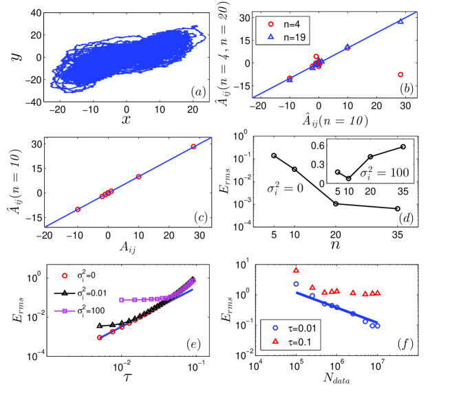
Figure 1: Application of VELSA to Lorenz system. (a) Trajectories of noisy system with $\sigma_{i}^{2}=100$ and time step for simulation being $10^{-4}$. (b-f) Reconstruction results with $n=10$, $N_{data}=10^{7}$ and $\tau=0.1$. (b) Reconstruction results $\hat{A}_{ij}$ with $n=4$ (the first order truncation) and $n=20$ (the third order truncation) plotted against those with $n=10$ (the second order truncation). (c) Reconstructed results of $\hat{A}_{ij}$ and $\hat{D}_{ij}$ plotted against the actual coefficients. (d) Dependence of $E_{rms}$ on the basis number $n$ with noise $\sigma_{i}^{2}=0$ and $\sigma_{i}^{2}=100$ (inset). (e) Dependence of $E_{rms}$ on $\tau$ with $\sigma_{i}^{2}=0,\ 0.01,\ 100$. (f) Dependence of $E_{rms}$ on the sampling number $N_{data}$ with $\tau=0.01$ and $\tau=0.1$. $\sigma_{i}^{2}=100$.

To show the effects of bases, we calculate the root mean square error

$$E_{rms}=\sqrt{\frac{\sum_{i=1}^{m}\sum_{j=1}^{n}(\hat{A}_{ij}-A_{ij})^{2}}{m\times n}},$$ (23)

Figure 1(d) presents $E_{rms}$ with noise $\sigma_{i}^{2}=0$ and $\sigma_{i}^{2}=100$ (inset). The bases of $n=5$ are the actual bases of Eq. (21), i.e., $x,\ y,\ z,\ xy,\ xz$. In Fig. 1(d) we observe that errors of the noise-free system monotonically decrease with $n$, while due to noise effects the results show an optimal and minimal error at about $n=10$ (small frame). Figure 1(e) shows the dependence of $E_{rms}$ on $\tau$ with $\sigma_{i}^{2}=0,\ 0.01,\ 100$. We observe that results with $\sigma_{i}^{2}=0$ (circles) well coincide with the line of $E_{rms}\propto\tau^{2}$ for small $\tau$. For finite noises, errors decrease with the decrease of $\tau$, however, the decreasing tendencies saturate at small $\tau$’s to finite errors depending on noise intensities. In Fig. 1(f) Error dependences of the sampling number $N_{data}$ with $\tau=0.01$ (circles) and $\tau=0.1$ (squares) are plotted. The results of $\tau=0.01$ monotonically decrease, approximately proportional to $\frac{1}{\sqrt{N_{data}}}$. However, errors for $\tau=0.1$ tend to saturation, which is determined by low measurement frequency. The $E_{rms}$ behaviors in both Figs. (e)(f) clearly show the different effects of $\sigma_{i}$, $\tau$ and $N_{data}$, and the competitive rules of $N_{data}^{-\frac{1}{2}}$, $\sigma_{i}$ and $\tau^{2}$ for $E_{rms}$. For detailed software codes of the method, see Ref. 26 .

Figure 2: Trajectories of Eq. (5) with no noise ((a)) and noise impacts $\sigma_{i}^{2}=100$ ((b)). $n=10$. Variables have no residual terms in their corresponding equations in top and middle panels while they do have in bottom panels. Solid-red and dash-blue curves are reconstructed and actual trajectories, respectively. Both types of curves coincide with each other perfectly when the corresponding equations have no residual terms, and small fluctuations are observed while nonzero residual terms exist.

For examining the validity of Eq. (12) we compare the reconstruction trajectories of Eq. (5) by setting $e(t)=0$ and the actual ones in Fig. 2. It is shown that without noise (Fig. 2(a)) the two trajectories are almost identical when $\dot{L}_{i}(t)$ equations do not contain residual term while small deviations are observed when residual exists. With noises (Fig. 2(b)) the above conclusions are still valid, but reconstruction curves show some fluctuations caused by noises.

For demonstrating effectiveness of Eq. (12) we plot the trajectories of reconstruction system in Fig.3(a) and 3(b), corresponding to noisy and noise-free reconstruction systems, respectively. Figure 3(c) shows the trajectories of an original noise-free system. From comparison of Fig. 3(a) and Fig. 1(a), Fig. 3(b) and 3(c), we draw a conclusion that using our VELSA method not only reconstructs the noisy system, but also predicts the noise-free system.

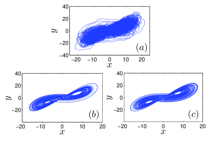
Figure 3: Trajectories of Lorenz systems. Reconstruction system of an original noisy system with reconstructed noises (a) and without noises (b). Original noise impacts $\sigma_{i}^{2}=100$. (c) Actual noise-free system.

III.2 A FHN neural network

We now consider a more complicated nonlinear network, the noisy FHN neural network,

$$\dot{v_{i}} = \frac{1}{\epsilon}(v_{i}-\frac{1}{3}v_{i}^{3}-u_{i}+I)+\sum_{j=1}^{N}c_{ij}(v_{j}-v_{i})+\eta_{1}(t),$$

$$\dot{u_{i}} = \gamma v_{i}-u_{i}+b+\eta_{2}(t),$$ (24)

where we take $\epsilon=0.1$, $I=0$, $\gamma=b=1.5$ and $N=10$. Noise $\sigma_{i}^{2}=0.1,i=1,\ 2$. $c_{ij}$ are coupling strengths generated from the connection coefficients with connection probability $0.3$ and the weighted coefficients uniformly distributed in $[0.4,\ 4.0]$. Here we separately define coupling coefficients as $c_{ij}$, and local dynamic coefficients in Eq. (3) as $f_{ij}$, $\dot{v}_{i}=f_{iv}(v,u)$, $\dot{u}_{i}=f_{iu}(v,u)$. We can reconstruct $\hat{c}_{ij}$ and $\hat{f}_{ij}$ plotted in Figs. 4(a)(b), and satisfactory identities are observed.

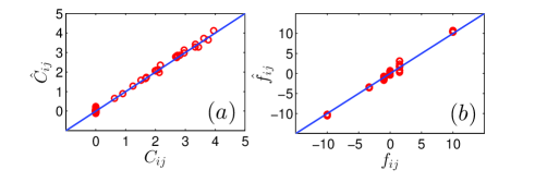
Figure 4: Reconstruction of a 10-node FHN network. Reconstructed $\hat{c}_{ij}$ and $\hat{f}_{ij}$ plotted against actual $c_{ij}$ (a) and $f_{ij}$ (b). Variables are taken up to the third order of power expansion. $\tau=0.1$. $N_{data}=4\times 10^{6}$.

IV Comparison and Discussion

After all the above demonstration of network reconstructions, a detailed comparisons between the VELSA method and the two previous methods are in order. Here the main problem in the present study is the joint difficulties of (i) Nonlinearity; (ii) Noise; (iii) Low measurement frequency. In [22], authors considered (i) and (ii) together with very fast data measurement such that velocities of $\textbf{x}(t)$ can be accurately computed. In [23] authors considered (ii) and (iii) together by considering trajectories around a fixed point where network dynamics can be directly treated with linear approximations. Both methods fail if all difficulties of (i), (ii) and (iii) appear together.In Fig. 5(a), we compare the results of reconstruction of Eq. (21). While VELSA shows low $E_{rms}$ for rather wide $\tau$ range, the method HOCC in 22 produces large errors. In Fig. 5(b) we compare the results of reconstruction of Eq. (24), and it is clearly shown that while VELSA satisfactorily infers all the network links, the method in 23 fails to do so.

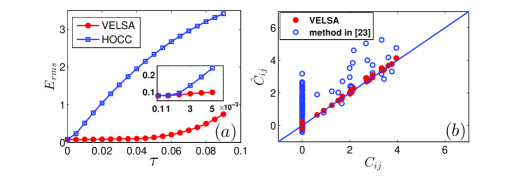
Figure 5: Comparison of three methods. (a) Dependence of $E_{rms}$ on $\tau$ for HOCC 22 and VELSA. (b) Calculated results $\hat{c}_{ij}$ plotted against the actual coefficients $c_{ij}$ for the method in 23 and VELSA.

For treating reconstruction problem of nonlinear and noisy network Eq. (1), the VELSA method (i) Transfers nonlinear terms of network Eq. (1) to expanded variables of equivalent linear network Eq. (4) while it is not closed; (ii) Uses the least squares approximations Eq. (6) to close the expanded linear network Eq. (4), i.e., to derive Eq.(5); (iii) Analytically solves Eq. (5) through two-time correlations by decomposing effects of system dynamics and noise impacts. Numerical computations fully justify the least squares approximations (Fig. 2), and the efficiency of reconstruction computation Eq. (12) (Figs. 1(b)(c), Fig.3 and Fig. 4).

With the above method we can achieve the following: (i) Though the reconstruction is applied for purely linear network Eq. (5), it fully includes strongly nonlinear effects (see Figs. 2, 3 and 4) due to that all nonlinear terms are taken into account in different expanded variables of Eq.(5) (in variables of $n\geq m$), and this is essentially different from linearization in conventional sense (e.g., see the comparison in Fig. 5(b)); (ii) Due to the utilization of analytical solution of linearized network Eq. (12), this method can obtain much better results when the measurement frequency is relatively low (see the analysis of Eq. (A10) and the comparison in Fig. 5(a)); (iii) The VELSA method can infer with measurable data not only the network structure in Eq. (12), but also noise statistical matrix D in Eq. (17). Then with the reconstructed network we can predict the behaviors of the original network without subjecting noises (see Figs. 3(b)(c)), and reproduce the behaviors of the actual network under the impacts of realistic noises (compare Figs.1(a) and 3(a)).

The proposed method can be applied in real systems to infer network structures under certain conditions. At the present stage the VELSA method has its own limitations restricting the practical applications of the method. First, we consider white noise approximations for treating fast-varying noises. Extensions to slow-varying noises or even to noises with wide spectra should be further investigated. Second, this method usually includes large number of unknown parameters to be reconstructed, and thus need large data sets in computations, and small data sets can cause large errors (see circles in Fig. 1(f)). How to improve reconstruction precision when data sets are relatively small is still an important and unsolved problem. Third, the VELSA method can well treat data collected with much lower measurement frequency, in comparison with all the methods where time-derivatives from data are needed for reconstructions (Fig. 5(a)). However, this capability is limited either. By decreasing measurement frequency $\frac{1}{\tau}$, the reconstruction errors increase and the method completely fail at very large $\tau$ (see triangles in Fig. 1(f)). Finally, in this paper we consider available data of all nodes in the dynamical network under investigation. The extension of the VELSA method to the cases with some nodes hidden is another subject of practical importance.

V Conclusion

In conclusion, we have proposed a method to reconstruct noisy nonlinear networks with fairly low measurement frequency, including all dynamic nonlinearities, network links, and noise statistical characteristics. Our method linearizes the original nonlinear equations by using expanded variables and solving nonlinear dynamics becomes equivalent to solving linear dynamics at the least squares approximations. Numerical results fully verify the validity of theoretical derivations and error analysis.

*

Appendix A ERROR DERIVATION

Preliminaries. The exponential of a matrix A is defined by

$$e^{\textbf{A}}=\sum_{k=0}^{\infty}\frac{1}{k!}\textbf{A}^{k}.$$ (A.1)

The logarithm of a matrix A is defined by

$$\ln(\textbf{I}-\textbf{A})=\sum_{k=1}^{\infty}\frac{(-1)^{k}}{k}\textbf{A}^{k}.$$ (A2)

where I is an identity matrix and the eigenvalues of A satisy the form $|\lambda|<1$.

Taylor expansion for an integration is defined by

$$\int_{t}^{t+\tau}F(s)L(s)ds=F(t)L(t)\tau+F^{(1)}(t)L(t)\frac{\tau^{2}}{2}$$ (A3)

$$+F(t)L^{(1)}\frac{\tau^{2}}{2}+O(\tau^{3})$$

where $F^{(1)}(t)$ and $L^{(1)}(t)$ are the first derivatives of $F(t)$ and $L(t)$ against $t$, respectively.

Error derivation. Considering the residual errors of expanded variables, i.e., $\textbf{e}(t)$, we have

$$\textbf{S}_{\tau}=e^{\textbf{B}\tau}\textbf{S}_{0}+\langle\int_{t}^{t+\tau}e^{\textbf{B}(t+\tau-s)}\textbf{e}(s)\textbf{L}(t)^{T}ds\rangle$$

With right multiplying $\textbf{S}_{0}^{-1}$, the above formulas yields

$$\textbf{S}_{\tau}\textbf{S}_{0}^{-1}=e^{\textbf{B}\tau}+\langle\int_{t}^{t+\tau}e^{\textbf{B}(t+\tau-s)}\textbf{e}(s)\textbf{L}(t)^{T}ds\rangle\textbf{S}_{0}^{-1}$$ (A4)

Define

$$\textbf{C}=\langle\int_{t}^{t+\tau}e^{\textbf{B}(t+\tau-s)}\textbf{e}(s)\textbf{L}(t)^{T}ds\rangle\textbf{S}_{0}^{-1},$$ (A5)

then $\textbf{S}_{\tau}\textbf{S}_{0}^{-1}=e^{\textbf{B}\tau}+\textbf{C}$. We transform it into

$$\textbf{B}\tau=\ln(\textbf{S}_{\tau}\textbf{S}_{0}^{-1}-\textbf{C}).$$ (A6)

First we compute the integration term in C, $\int_{t}^{t+\tau}e^{\textbf{B}(t+\tau-s)}\textbf{e}(s)ds$. By using Eq. (A3), Taylor expansion yields

$$\int_{t}^{t+\tau}e^{\textbf{B}(t+\tau-s)}\textbf{e}(s)ds=e^{\textbf{B}\tau}\textbf{e}(t)\tau-\textbf{B}e^{\textbf{B}\tau}\textbf{e}(t)\frac{1}{2}\tau^{2}$$

$$+e^{\textbf{B}\tau}\textbf{e}^{(1)}(t)\frac{1}{2}\tau^{2}+O(\tau^{3})$$

and Eq. (A5) becomes

$$\textbf{C}=e^{\textbf{B}\tau}[\langle\textbf{e}(t)\textbf{L}(t)^{T}\rangle\tau-\textbf{B}\langle\textbf{e}(t)\textbf{L}(t)^{T}\rangle\frac{\tau^{2}}{2}+\langle\textbf{e}^{(1)}(t)\textbf{L}(t)^{T}\rangle\frac{\tau^{2}}{2}+O(\tau^{2})]$$ (A7)

By using Eq. (A3), we further arrive at

$$\langle\int_{t}^{t+\tau}\textbf{e}(s)\textbf{L}(s)^{T}ds\rangle=\langle\textbf{e}(t)\textbf{L}(t)^{T}\rangle\tau+\langle\textbf{e}^{(1)}(t)\textbf{L}(t)^{T}\rangle\frac{\tau^{2}}{2}+\langle\textbf{e}(t)\textbf{L}^{(1)}(t)^{T}\rangle\frac{\tau^{2}}{2}+O(\tau^{3})$$

Due to the least squares approximations

$$\frac{1}{T_{2}-T_{1}}\int_{T_{1}}^{T_{2}}\textbf{e}(s)\textbf{L}(s)^{T}ds=\langle\frac{\int_{t}^{t+\tau}\textbf{e}(s)\textbf{L}(s)^{T}ds}{\tau}\rangle=0,$$

we have

$$\langle\textbf{e}(t)\textbf{L}(t)^{T}\rangle\tau+\langle\textbf{e}^{(1)}(t)\textbf{L}(t)^{T}\rangle\frac{\tau^{2}}{2}$$

$$=-\langle\textbf{e}(t)\textbf{L}^{(1)}(t)^{T}\rangle\frac{\tau^{2}}{2}+O(\tau^{3})$$

and

$$\langle\textbf{e}(t)\textbf{L}(t)^{T}\rangle=O(\tau)$$

Basing on the above two transformations, we rewrite C as

$$\textbf{C}=-e^{\textbf{B}\tau}\langle\textbf{e}(t)\textbf{L}^{(1)}(t)^{T}\rangle\frac{\tau^{2}}{2}\textbf{S}_{0}^{-1}+O(\tau^{3})$$ (A8)

Further transforming Eq. (A6) into $\textbf{B}\tau=\ln(\textbf{I}-(\textbf{I}-\textbf{S}_{\tau}\textbf{S}_{0}^{-1}+\textbf{C}))$, considering small $\tau$, we have $\textbf{S}_{\tau}\textbf{S}_{0}^{-1}\approx\textbf{I}$. Together with Eq. (A2), we can derive

$$\ln(\textbf{I}-(\textbf{I}-\textbf{S}_{\tau}\textbf{S}_{0}^{-1}+\textbf{C})) = \sum_{n=1}^{\infty}\frac{(-1)^{n}}{n}(\textbf{I}-\textbf{S}_{\tau}\textbf{S}_{0}^{-1}+\textbf{C})^{n}$$

$$= \sum_{n=1}^{\infty}\frac{(-1)^{n}}{n}(\textbf{I}-\textbf{S}_{\tau}\textbf{S}_{0}^{-1})^{n}-\textbf{C}+\frac{1}{2}(\textbf{I}-\textbf{S}_{\tau}\textbf{S}_{0}^{-1})\textbf{C}+\frac{1}{2}\textbf{C}(\textbf{I}-\textbf{S}_{\tau}\textbf{S}_{0}^{-1})+O(\textbf{C}^{2})$$

$$= \ln\textbf{S}_{\tau}\textbf{S}_{0}^{-1}-\textbf{C}+\frac{1}{2}(\textbf{I}-\textbf{S}_{\tau}\textbf{S}_{0}^{-1})\textbf{C}+\frac{1}{2}\textbf{C}(\textbf{I}-\textbf{S}_{\tau}\textbf{S}_{0}^{-1})+O(\textbf{C}^{2})$$

Since $\textbf{C}=O(\tau^{2})$ (Eq. (A8)) and $(\textbf{I}-\textbf{S}_{\tau}\textbf{S}_{0}^{-1})=O(\tau)$ (Eq. (A4)), we have

$$\textbf{B}\tau=\ln\textbf{S}_{\tau}\textbf{S}_{0}^{-1}-\textbf{C}+O(\tau^{3})$$ (A9)

Substituting Eq. (A8) into Eq. (A9), we finally obtain the error of reconstruction

$$\textbf{B}-\hat{\textbf{B}}=e^{\textbf{B}\tau}\langle\textbf{e}(t)\textbf{L}^{(1)}(t)^{T}\rangle\textbf{S}_{0}^{-1}\frac{\tau}{2}+O(\tau^{2}).$$ (A10)

where reconstructed matrix $\hat{\textbf{B}}=\frac{\ln(\textbf{S}_{\tau}\textbf{S}_{0}^{-1})}{\tau}$.

References

- (1) J.M. Stuart, E. Segal, D. Koller, and K.K. Stuart, A gene-coexpression network for global discovery of conserved genetic modules, Science 302, 249 (2003).
- (2) A.J. Butte, P. Tamayo, D. Slonim, T.R. Golub, and I.S. Kohane, Discovering functional relationships between RNA expression and chemotherapeutic susceptibility using relevance networks, Proceedings of the National Academy of Sciences 97(22), 12182 (2000).
- (3) A. Fuente, N. Bing, I. Hoeschele, and P. Mendese, Discovery of meaningful associations in genomic data using partial correlation coefficients, Bioinformatics 20(18), 3565 (2004).
- (4) J.J. Faith, B. Hayete, J.T. Thaden, I. Mogno, J. Wierzbowski et al., Large-scale mapping and validation of Escherichia coli transcriptional regulation from a compendium of expression profiles, PLoS Biol 5(1), e8 (2007).
- (5) P.E. Meyer, K. Kontos, F. Lafitte, and G. Bontempi, Information-theoretic inference of large transcriptional regulatory networks, EURASIP J Bioinform Syst Biol. 2007, 79879 (2007).
- (6) P.E. Meyer, D. Marbach, S. Roy, and M. Kellis, Information-Theoretic Inference of Gene Networks Using Backward Elimination, Biocomp 700-705. 102 (2010).
- (7) A.A. Margolin, I. Nemenman, K. Basso, C. Wiggins, G. Stolovitzky, R. D. Favera, and A. Califano, ARACNE: an algorithm for the reconstruction of gene regulatory networks in a mammalian cellular context, BMC bioinformatics 7: S7 (2006).
- (8) D. Heckerman, A tutorial on learning with Bayesian networks, Springer, 301-354 (1998).
- (9) I. Tsamardinos, C. F. Aliferis, A. Statnikov, Time and sample efficient discovery of Markov blankets and direct causal relations, Proceedings of the ninth ACM SIGKDD international conference on Knowledge discovery and data mining 673-678 (2003).
- (10) D. Yu, M. Righero, and L. Kocarev, Estimating topology of networks, Phys. Rev. Lett. 97(18), 188701 (2006).
- (11) M. Timme, Revealing network connectivity from response dynamics, Phys. Rev. lett. 98(22), 224101 (2007).
- (12) S. G. Shandilya, and M. Timme, Inferring network topology from complex dynamics, New J. of Phys. 13(1), 013004 (2011).
- (13) W.X. Wang, R. Yang, Y.C. Lai, V. Kovanis, and C. Grebogi, Predicting catastrophes in nonlinear dynamical systems by compressive sensing, Phys. Rev. Lett. 106(15), 154101 (2011).
- (14) Z. Levnaji, and A. Pikovsky, Untangling complex dynamical systems via derivative-variable correlations, Sci. Rep. 4, 5030 (2014).
- (15) V.N. Smelyanskiy, D.G. Luchinsky, D.A. Timu?in, and A. Bandrivskyy, Reconstruction of stochastic nonlinear dynamical models from trajectory measurements, Phys. Rev. E 72(2), 026202 (2005).
- (16) V.N. Smelyanskiy, D.G. Luchinsky, A. Stefanovska, and P.V.E. McClintock, Inference of a nonlinear stochastic model of the cardiorespiratory interaction. Phys. Rev. Lett. 94(9), 098101 (2005).
- (17) T. Stankovski, A. Duggento, and P.V. McClintock, A. Stefanovskaet, Inference of time-evolving coupled dynamical systems in the presence of nois, Phys. Rev. Lett. 109(2), 024101 (2012).
- (18) J. Ren, W.X. Wang, B.W. Li, and Y.C. lai, Noise bridges dynamical correlation and topology in coupled oscillator networks, Phys. Rev. Lett. 104(5), 058701 (2010).
- (19) W.X. Wang, J. Ren, Y.C. Lai, and B.W. Li, Reverse engineering of complex dynamical networks in the presence of time-delayed interactions based on noisy time series, Chaos 22(3), 033131 (2012).
- (20) Z.Y. Zhang, Z.G. Zheng, H.J. Niu, Y.Y. Mi, S. Wu,and G. Hu, Solving the inverse problem of noise-driven dynamic networks, Phys. Rev. E 91(1), 012814 (2015).
- (21) Y. Chen, S.H. Wang, Z.G. Zheng, Z.Y. Zhang, and G. Hu, Depicting network structures from variable data produced by unknown colored-noise driven dynamics, Europhys. Lett. 113, 18005 (2016).
- (22) Y. Chen, Z.Y. Zhang, T.Y. Chen, S.H. Wang, and G. Hu, Reconstruction of noise-driven nonlinear networks from node outputs by using high-order correlations, Sci. Rep. 7, 44639 (2017).
- (23) S.C. Emily, H.C. Tam, Reconstructing links in directed networks from noisy dynamics. Phys. Rev. E 95, 010301(R) (2017).
- (24) P.K. Lai, Reconstructing network topology and coupling strengths in directed networks of discrete-time dynamics, Phys. Rev. E 95, 022311 (2017).
- (25) T. Stankovski, T. Pereira, P.V.E. McClintock, A. Stefanovska, Coupling functions: Universal insights into dynamical interaction mechanisms, in press in Reviews of Modern Physics.
- (26) Two software codes based on MATLAB, are used to produce data from noisy Lorenz system and reconstruct the model from the data above by using our method proposed, respectively. http://blog.csdn.net/SrdLaplace/article/details/78283343