Indirect Image Registration with Large Diffeomorphic Deformations

Abstract

The paper adapts the LDDMM framework for image registration to the indirect setting where a template is registered against a target that is given through indirect noisy observations. The registration uses diffeomorphisms that transform the template through a (group) action. These diffeomorphisms are generated by solving a flow equation that is defined by a velocity field with certain regularity. The theoretical analysis includes a proof that indirect image registration has solutions (existence) that are stable and that converge as the data error tends so zero, so it becomes a well-defined regularization method. The paper concludes with examples of indirect image registration in 2D tomography with very sparse and/or highly noisy data.

65F22, 65R32, 65R30, 65D18, 94A12, 94A08, 92C55, 54C56, 57N25, 47A52

1 Introduction

Image registration (matching) is the task of transforming a template image so that it matches a target image. This arises in many fields, such as quality control in industrial manufacturing [27], various applications in remote sensing [25], face recognition [67, 51], robotic navigation [14], and medical imaging [57, 53, 60], etc. The variant that is considered here is indirect image registration, i.e., when the template image is registered against a target that is known only through indirect noisy observations, such as in tomographic imaging. It makes use of the LDDMM framework for diffeomorphic image registration and thereby extends the indirect image registration scheme in [46], which uses (small) linearized deformations.

An important development in regularization theory is ongoing where reconstruction and feature extraction steps are pursued simultaneously, such as joint segmentation and reconstruction. Indirect image registration can be seen as part of this development where the feature in question is the “shape” of the structures in the image and their temporal variability. This is highly relevant for spatiotemporal imaging, see [46] for a survey and other use cases of indirect image registration.

There is an extensive literature on image registration where a template is registered by means of a diffeomorphism against a target so that their “shapes” agree, see [57] for a nice survey. Image registration is then recast as the problem of finding a suitable diffeomorphism that deforms the template into the target image [21]. The underlying assumption is that the target image is contained in the orbit of the template under the group action of diffeomorphisms. This principle can be stated in a very general setting where diffeomorphism acts on various image features, like landmark points, curves, surfaces, scalar images, or even vector/tensor valued images [65]. It also adapts readily to the indirect image registration setting and this is worked out in detail for the case when one seeks to register scalar images.

2 Overview of paper and specific contributions

The main contribution is to develop a variational framework for indirect image registration (Section 6) where a template is registered against a target that is known only through indirect noisy observations (data). This is done by appropriately adapting the LDDMM framework where the template is deformed by diffeomorphisms that act on images through a group action as explained in Section 5. This section also contains an overview of the LDDMM theory.

An important theoretical topic is to investigate to what extent this indirect registration scheme is a regularization. Existence of solutions along with stability and convergence results are stated in Section 7. In conclusion, the LDDMM based indirect registration scheme is formally a well-defined regularization method. On the other hand, as most of the other variational schemes for image registration, one cannot expect to have uniqueness due to lack of convexity. This theoretical investigation is followed by explicit calculations of the derivative and gradient of the objective functional in the variational formulation of the indirect registration problem (Section 8). Numerical implementation, which relies on theory of RKHS (Section 4) is outlined in Section 9.

Section 10 contains some numerical experiments from tomography that show performance of indirect image registration. The results support the claim that shape information contained in the template has a strong regularizing effect, and especially so for noisy highly under-sampled inverse problems. Furthermore, the experiments also suggest that the prior shape information does not have to be that accurate, which is important for the used cases mentioned in [46]. None of these claims are however proved formally by mathematical theorems.

Finally, Section 11 discusses possible extensions of indirect image registration to the case when the template also needs to be recovered. It also outlines how indirect image registration relates to joint reconstruction and motion estimation in spatiotemporal imaging.

3 Inverse problems, ill-posedness and variational regularization

The purpose of this section is to set some notations and concepts used throughout the paper.

Image reconstruction

The goal in image reconstruction is to estimate some spatially distributed quantity (image) from indirect noisy observations (measured data). Stated mathematically, the aim is to reconstruct an image $f_{\text{true}}\in X$ from data $g\in Y$ where

(1) $$g=\mathcal{T}(f_{\text{true}})+\Delta g.$$

Here, $X$ (reconstruction space) is the vector space of all possible images, so it is a suitable Hilbert space of functions defined on a fixed domain $\Omega\subset\mathbb{R}^{n}$. Next, $Y$ (data space) is the vector space of all possible data, which for digitized data is a subset of $\mathbb{R}^{m}$. Furthermore, $\mathcal{T}\colon X\to Y$ (forward operator) models how a given image gives rise to data in absence of noise and measurement errors, and $\Delta g\in Y$ (data noise component) is a sample of a $Y$–valued random element whose probability distribution is (data noise model) assumed to be explicitly expressible in terms of $\mathcal{T}(f_{\text{true}})$.

Ill-posedness

A naive approach for reconstructing the true (unknown) image $f_{\text{true}}$ is to solve the equation $\mathcal{T}(f)=g$. Often there are no solutions to this equation since measured data is not in the range of $\mathcal{T}$ for a variety of reasons (noise, modeling errors, etc.). This is commonly addressed by relaxing the notion of a solution by considering

(2) $$\min_{f\in X}\mathcal{D}\bigl{(}\mathcal{T}(f),g\bigr{)}.$$

The mapping $\mathcal{D}\colon Y\times Y\to\mathbb{R}$ (data discrepancy functional) quantifies the data misfit and a natural candidate is to choose it as a suitable affine transformation of the negative log likelihood of data. In such case, solving Eq. 2 amounts to finding ML solutions, which works well when Eq. 2 has a unique solution (uniqueness) that depends continuously on data (stability). This is however not the case when Eq. 1 is ill-posed, in which case one needs to use regularization that introduces stability, and preferably uniqueness, by making use of prior knowledge about $f_{\text{true}}$.

Variational regularization

The idea here is to add a penalization term to the objective functional in Eq. 2 resulting in a variational problem of the type

(3) $$\min_{f\in X}\Bigl{[}\mu\mathcal{R}(f)+\mathcal{D}\bigl{(}\mathcal{T}(f),g\bigr{)}\Bigr{]}\quad\text{for some given $\mu\geq 0$.}$$

Such regularization methods have gained much attention lately, and especially so in imaging [52]. The functional $\mathcal{R}\colon X\to\mathbb{R}$ introduces stability, and preferably also uniqueness, often by encoding some priori known regularity property of $f_{\text{true}}$, e.g., assuming $X\subset\mathscr{L}^{2}(\Omega,\mathbb{R})$ and taking the $\mathscr{L}^{2}$-norm of the gradient magnitude (Dirichlet energy) is known to produce smooth solutions whereas taking the $\mathscr{L}^{1}$-norm of the gradient magnitude (TV) yields solutions that preserve edges while smooth variations may be suppressed [18].

4 Reproducing kernel Hilbert spaces

The diffeomorphic deformations constructed in the LDDMM framework (Section 5.3.1) will make use of velocity fields that at each time point are contained in a RKHS. The gradient computations in Section 8 also rely on this assumption. The short introduction to the theory of RKHS provided here gives the necessary background needed in subsequent sections.

The theory of RKHS was initialized in the 1940s for spaces of scalar-valued functions [4], which was later extended to spaces of functions with values in locally convex topological spaces [55]. It has lately gained significant interest due to applications in machine learning [54, 12, 44]. The starting point is an abstract Hilbert space $H$ whose elements are functions defined on a fixed domain $\Omega\subset\mathbb{R}^{n}$ that take values in a real Hilbert space $U$. Such a space is a RKHS if evaluation functionals $\delta^{a}_{x}\colon H\to\mathbb{R}$ defined as $\delta^{a}_{x}(\nu):=\bigl{\langle}\nu(x),a\bigr{\rangle}_{U}$ are bounded for every $x\in\Omega$ and $a\in U$. One way to construct a RKHS is to specify a reproducing kernel function. It maps a pair of points in $\Omega$ into the Banach space $\mathscr{L}(U,U)$ of bounded linear operators on $U$, i.e., an operator $\mathcal{K}\colon\Omega\times\Omega\to\mathscr{L}(U,U)$ such that

1. $\mathcal{K}(\,\cdot\,,x)(a)\in H$ for all $x\in\Omega$ and $a\in U$.

2. The reproducing property holds for $\mathcal{K}$, i.e., if $x\in\Omega$ then

   (4) $$\bigl{\langle}\nu(x),a\bigr{\rangle}_{U}=\bigl{\langle}\nu,\mathcal{K}(\,\cdot\,,x)(a)\bigr{\rangle}_{H}\quad\text{for any $\nu\in H$ and $a\in U$.}$$

An important characterization is that a Hilbert space $H$ of $U$-valued functions that is continuously embedded in $\mathscr{C}(\Omega,U)$ is a RKHS if and only if it has a continuous reproducing kernel $\mathcal{K}\colon\Omega\times\Omega\to\mathscr{L}(U,U)$.

Square integrable vector fields

If $H$ is a Hilbert space of vector fields on $\mathbb{R}^{n}$ that is admissible (see Section 5.3.1), then it is in particular continuously embedded in $\mathscr{C}(\Omega,\mathbb{R}^{n})$. Hence, it is a RKHS if and only if it has a continuous positive definite reproducing kernel $\mathcal{K}\colon\Omega\times\Omega\to\mathscr{L}(\mathbb{R}^{n},\mathbb{R}^{n})$, which in turn can be represented by a continuous positive definite function $\mathsf{K}\colon\Omega\times\Omega\to\mathbb{M}_{+}^{n\times n}$. Here, $\mathbb{M}^{n,m}$ denotes the vector space of all $(n\times m)$ matrices and $\mathbb{M}^{n,m}_{+}$ denotes those matrices that are positive definite. Assuming in addition that $H$ is a RKHS that is continuously embedded in $L^{2}(\Omega,\mathbb{R}^{n})$, then there exists an continuous imbedding $\iota\colon H\to\mathscr{L}^{2}(\Omega,\mathbb{R}^{n})$. Hence, by Riesz theorem there exist $\iota^{*}\colon\mathscr{L}^{2}(\Omega,\mathbb{R}^{n})\to H$ such that

(5) $$\bigl{\langle}\iota(\nu),\eta\bigr{\rangle}_{\mathscr{L}^{2}(\Omega,\mathbb{R}^{n})}=\bigl{\langle}\nu,\iota^{*}(\eta)\bigr{\rangle}_{H}\quad\text{for all $\nu,\eta\in H$}.$$

A natural task is to further examine the relation between the $\mathscr{L}^{2}$-inner product and the RKHS inner product on $H$. As we next show, one can prove that

(6) $$\langle\eta,\nu\rangle_{\mathscr{L}^{2}}=\Bigl{\langle}\nu,\int_{\Omega}\mathcal{K}(\,\cdot\,,x)\bigl{(}\eta(x)\bigr{)}\,\text{d}x\Bigr{\rangle}_{H}.$$

To prove Eq. 6, observe first that by Eq. 5

$$\bigl{\langle}\iota(\nu),\iota(\eta)\bigr{\rangle}_{\mathscr{L}^{2}(\Omega,\mathbb{R}^{n})}=\Bigl{\langle}\nu,\iota\bigl{(}\iota^{*}(\eta)\bigr{)}\Bigr{\rangle}_{H}\quad\text{for any $\nu,\eta\in H$.}$$

Hence, Eq. 6 follows directly from

(7) $$\iota\bigl{(}\iota^{*}(\eta)\bigr{)}=\int_{\Omega}\mathcal{K}(\,\cdot\,,x)\bigl{(}\eta(x)\bigr{)}\,\text{d}x.$$

To prove Eq. 7, observe first that it is sufficient to prove it point wise, i.e., to show that

(8) $$\Bigl{\langle}\iota\bigl{(}\iota^{*}(\eta)\bigr{)}(y),a\Bigr{\rangle}_{\mathbb{R}^{n}}=\int_{\Omega}\Bigl{\langle}\mathcal{K}(y,x)\bigl{(}\eta(x)\bigr{)},a\Bigr{\rangle}_{\mathbb{R}^{n}}\,\text{d}x\quad\text{holds for any $y\in\Omega$ and $a\in\mathbb{R}^{n}$.}$$

The equality in Eq. 8 follows from the next calculation:

$$\Bigl{\langle}\iota\bigl{(}\iota^{*}(\eta)\bigr{)}(y),a\Bigr{\rangle}_{\mathbb{R}^{n}} =\bigl{[}\text{By \lx@cref{creftype~refnum}{eq:IpEquality}}\bigr{]}=\Bigl{\langle}\iota^{*}\bigl{(}\iota(\eta)\bigr{)},\mathcal{K}(\,\cdot\,,y)(a)\Bigr{\rangle}_{H}\!=\!\bigl{[}\text{By \lx@cref{creftype~refnum}{eq:Inclusion}}\bigr{]}\!\!=\Bigl{\langle}\iota(\eta),\iota\bigl{(}\mathcal{K}(\,\cdot\,,y)(a)\bigr{)}\Bigr{\rangle}_{\mathscr{L}^{2}}$$

$$=\int_{\Omega}\Bigl{\langle}\iota(\eta)(x),\iota\bigl{(}\mathcal{K}(\,\cdot\,,y)(a)\bigr{)}(x)\Bigr{\rangle}_{\mathbb{R}^{n}}\,\text{d}x=\int_{\Omega}\Bigl{\langle}\eta(x),\mathcal{K}(x,y)(a)\Bigr{\rangle}_{\mathbb{R}^{n}}\,\text{d}x.$$

LDDMM

5 Shape theory

The overall aim is to develop a quantitative framework for studying shapes and their variability. The approach considered here is based on deformable templates and it can be traced back to work by D’Arcy Thompson in beginning of 1900’s [24]. Shape theory based on deformable templates is now an active field of research [31, 65, 58, 43].

The starting point is to specify a shape space, which here refers to a set whose elements are image features with shapes that are to be analysed. There is no formal definition of what constitutes an image feature, but intuitively it is a representation of the image that retains information relevant for its interpretation. Hence, the choice of shape space is highly task dependent and examples are landmark points, curves, surfaces, and scalar/vector/tensor valued images. This is followed by specifying a set of deformations whose elements map the shape space into itself and thereby model shape changes. Clearly, the identity mapping preserves all aspects of shape. And in this context, it is therefore the “smallest” deformation. A key step will be to introduce a metric on the set of deformations that induces a shape similarity measure in shape space.

5.1 Shape space

There are many image features important for interpretation [7], see also [38, 39] for an axiomatic characterization of features natural for visual perception. For (indirect) image registration, it is important that such features are deformable. Namely, it should be feasible to act on it by means of a deformation.

This paper considers grey-scale images, more precisely $X=SBV(\Omega,\mathbb{R})\bigcap\mathscr{L}^{\infty}(\Omega,\mathbb{R})$. The requirement that elements in $X$ are in $\mathscr{L}^{\infty}(\Omega,\mathbb{R})$ (essentially bounded) is reasonable for images since grey-scale values are bounded. Furthermore, $SBV(\Omega,\mathbb{R})$ denotes the set of real-valued functions of special bounded variation over $\Omega\subset\mathbb{R}^{n}$. This space was first introduced in [3] (see also [26]) and its formal definition is somewhat involved, see [59, Definition 22 on p. 141]. Intuitively, these are functions of bounded variation whose singular part of the distributional derivative is supported by an $(n-1)$-dimensional rectifiable set in $\Omega$. In particular, such functions are not necessarily smooth. The latter is important since images may contain edges. Occasionally $X$ will be equipped with an $\mathscr{L}^{2}$–inner product.

5.2 Set of deformations

Deformations are operations that transform elements in a shape space. In our setting, deformations is represented by mappings from the image domain $\Omega\subset\mathbb{R}^{n}$ into $\mathbb{R}^{n}$ along with an action describing how they deform deformable objects. The set of deformations should be rich enough to capture the shape variability arising in the application, yet restricted enough to allow for a coherent mathematical theory.

Considering only rigid body motions is often too limited since many applications involve non-rigid shape deformations. Furthermore, composing two deformations should yield a valid deformation, i.e., the set $G$ of deformations closed under composition. Here, the identity mapping becomes the natural “zero” deformation. Furthermore, it should also be possible to reverse a deformation, i.e., $G$ closed under inversion. Taken together, this implies that $G$ forms a group under the group law given by composition of functions. The group structure also implies that a deformation transforms an element in the shape space by means of a group action. Finally, often it also makes sense to assume that deformable objects do not tear, fold or collapse the image, i.e., the deformation preserving the topology.

$\mathscr{C}^{p}$-diffeomorphisms (see below) form a group of non-rigid transformations satisfying the above requirements. These mappings can also act on real valued functions as in Section 5.4.

$$\operatorname{Diff}^{p}(\mathbb{R}^{n}):=\Bigl{\{}\phi\in\mathscr{C}^{p}(\mathbb{R}^{n},\mathbb{R}^{n}):\text{$\phi$ is bijective with $\phi^{-1}\in\mathscr{C}^{p}(\mathbb{R}^{n},\mathbb{R}^{n})$}\Bigr{\}}.$$

However, formulating and proving mathematical results relevant for (indirect) image registration, and the need to perform computations with such objects, require one to further restrict the set of diffeomorphisms, i.e., considering suitable sub-groups of $\operatorname{Diff}^{p}(\mathbb{R}^{n})$.

5.3 Large diffeomorphic deformations

A natural approach is to consider deformations given by additively perturbing the identity map with a vector field that is sufficiently regular [46]. The resulting set of deformations is closed under composition, i.e., it forms a semi-group. Furthermore, such a deformation can be seen as linear approximation of a diffeomorphism, but it is not necessarily invertible unless the aforementioned vector field is sufficiently small and regular [65, Proposition 8.6]. Hence, this is not a suitable framework for diffeomorphic image registration where the template and target have large differences.

One approach to address the above issue of invertibility was presented in [21]. The idea is to consider transformations given as a composition of infinitesimally small linearised deformations. More precisely, diffeomorphic large deformations are obtained by integrating the identity map along a velocity field (curve of vector fields). If properly designed, the velocity field induces an isotopy (a curve of diffeomorphisms). Thereby, the set of velocity fields parametrises the set of deformations and a natural requirement is that velocity fields under consideration have integrable trajectories. This provides a framework for generating a rich sets of deformations, which then can be adapted to specific image registration problems by appropriately choosing the velocity fields.

The indirect image registration method in this paper is based on LDDMM, see Section 11.2 for a brief survey of alternative frameworks for large diffeomorphic deformations. In LDDMM, the velocity field is square integrable and its corresponding vector field at each time is contained in a fixed Hilbert space of vector fields that is an admissible RKHS. The deformations are generated by integrating the identity map along trajectories of such velocity fields and these form a sub-group of $\operatorname{Diff}^{1}(\mathbb{R}^{n})$, see Section 5.3.1 for more details. As shown there, this group can furthermore be equipped with a metric, which by a group action (Section 5.4) induces a metric on the shape space that can be used to quantify shape similarity (Section 6).

5.3.1 The LDDMM framework

The starting point in the LDDMM framework for large diffeomorphic deformations is to define the vector space of velocity fields that generate the diffeomorphisms. An important point is to show that these diffeomorphisms for a group. Another is to define a right invariant metric so that the group is a complete metric space w.r.t. this metric. The metric is later used to induce a metric on the shape space, which in turn is used as a regularizer in indirect image registration (Section 6). A key part of showing that indirect image registration is a well-defined regularization method (Section 7) is to relate convergence of velocity fields to convergence of corresponding diffeomorphisms.

Admissible vector fields and the flow equation

The idea in LDDMM is to generate large diffeomorphic deformations by solving a flow equation. This is only possible when the velocity field enjoys certain regularity that ensures the flow equation has a unique solution. More precisely, fix a domain $\Omega\subset\mathbb{R}^{n}$ and let $V\subset\mathscr{C}_{0}^{p}(\Omega,\mathbb{R}^{n})$ denote a $p$–admissible vector space of vector fields, i.e., $V$ can be continuously embedded into $\mathscr{C}_{0}^{p}(\Omega,\mathbb{R}^{n})$ under the topology induced by the $\|\,\cdot\,\|_{p,\infty}$–norm. Furthermore, let $\mathscr{L}^{q}([0,1],V)$ denote the vector space of velocity fields that are $\mathscr{L}^{q}$-integrable in time and belong to $V$ at any time point, i.e.,

(9) $$\mathscr{L}^{q}([0,1],V):=\Bigl{\{}\boldsymbol{\nu}\colon[0,1]\times\Omega\to\mathbb{R}^{n}:\boldsymbol{\nu}(t,\,\cdot\,)\in V\text{ and $\|\boldsymbol{\nu}\|_{\mathscr{L}^{q}([0,1],V)}<\infty$}\Bigr{\}}$$

with

$$\|\boldsymbol{\nu}\|_{\mathscr{L}^{q}([0,1],V)}:=\biggl{(}\int_{0}^{1}\bigl{\|}\boldsymbol{\nu}(t,\,\cdot\,)\bigr{\|}^{q}_{V}\,\text{d}t\biggr{)}^{1/q}\quad\text{for an integer $q\geq 1$.}$$

This is a normed vector space and if $V$ is a Hilbert space, then $\mathscr{L}^{2}([0,1],V)$ can also be equipped with a Hilbert space structure. Focus will henceforth be on the Hilbert space $\mathscr{L}^{2}([0,1],V)$, but some statements will involve $\mathscr{L}^{1}([0,1],V)$. The following theorem forms the basis of the LDDMM approach, see [65, Appendix C] for its proof.

Theorem 5.1 (Existence of flows).

Given $\boldsymbol{\nu}\in\mathscr{L}^{1}([0,1],V)$, there exists a unique continuous curve $[0,1]\ni t\mapsto\phi^{\boldsymbol{\nu}}_{0,t}\in\operatorname{Diff}^{p}(\mathbb{R}^{n})$ that satisfies the following flow equation:

(10) $$\begin{cases}\dfrac{d}{dt}\phi^{\boldsymbol{\nu}}_{0,t}(x)=\boldsymbol{\nu}\bigl{(}t,\phi^{\boldsymbol{\nu}}_{0,t}(x)\bigr{)}&\\[7.5pt] \phi^{\boldsymbol{\nu}}_{0,0}(x)=x.&\end{cases}\quad\text{for all $x\in\Omega$.}$$

By Theorem 5.1, $\phi^{\boldsymbol{\nu}}_{s,t}:=\phi^{\boldsymbol{\nu}}_{0,t}\circ(\phi^{\boldsymbol{\nu}}_{0,s})^{-1}$ becomes a well defined element in $\operatorname{Diff}^{p}(\mathbb{R}^{n})$ for any $s,t\in[0,1]$, and by [65, Proposition C.6] one gets

(11) $$\phi^{\boldsymbol{\nu}}_{s,t}=\phi^{\boldsymbol{\nu}}_{\tau,t}\circ\phi^{\boldsymbol{\nu}}_{s,\tau}\quad\text{and}\quad(\phi^{\boldsymbol{\nu}}_{s,t})^{-1}=\phi^{\boldsymbol{\nu}}_{t,s}\qquad\text{for any $0\leq s,\tau,t\leq 1$.}$$

Diffeomorphisms generated by flows

Assume $V\subset\mathscr{C}_{0}^{p}(\Omega,\mathbb{R}^{n})$ is a $p$-admissible Banach space and define

(12) $$G_{V}:=\Bigl{\{}\phi^{\boldsymbol{\nu}}_{0,1}\colon\Omega\to\mathbb{R}^{n}:\text{$\phi^{\boldsymbol{\nu}}_{0,1}$ solves \lx@cref{creftype~refnum}{eq:FlowEq} with $\boldsymbol{\nu}\in\mathscr{L}^{1}([0,1],V)$}\Bigr{\}}.$$

As already concluded, $G_{V}\subset\operatorname{Diff}^{p}(\Omega)$ is a sub-group. Next, the norm on $\mathscr{L}^{1}([0,1],V)$ can be used to define a (right invariant) metric $\text{d}_{G}\colon G_{V}\times G_{V}\to\mathbb{R}_{+}$ on $G_{V}$ as

(13) $$\text{d}_{G}(\phi,\psi):=\!\!\inf_{\begin{subarray}{c}\boldsymbol{\nu}\in\mathscr{L}^{1}([0,1],V)\\ \psi=\phi\circ\phi^{\boldsymbol{\nu}}_{0,1}\end{subarray}}\,\|\boldsymbol{\nu}\|_{\mathscr{L}^{1}([0,1],V)}\quad\text{for $\phi,\psi\in G_{V}$.}$$

With this construction, $(G_{V},\text{d}_{G})$ is a complete metric space whenever $V$ is $p$-admissible [65, Theorem 8.15]. The right invariance of the metric is important since

$$\text{d}_{G}(\phi,\psi)=\text{d}_{G}(\phi\circ\varphi,\psi\circ\varphi)\quad\text{for any $\varphi\in G_{V}$.}$$

Furthermore, with this metric one can prove existence of a minimizing velcocity field between two diffeomorphisms in $G_{V}$. More precisely, if $V$ is $p$-admissible, then by [65, Theorems 8.18 and 8.20], for any $\phi,\psi\in G_{V}$ there exists a velocity field $\boldsymbol{\nu}\in\mathscr{L}^{2}([0,1],V)$ such that

(14) $$\text{d}_{G}(\phi,\psi)=\|\boldsymbol{\nu}\|_{\mathscr{L}^{2}([0,1],V)}\quad\text{and}\quad\psi=\phi\circ\phi^{\boldsymbol{\nu}}_{0,1}.$$

Hence, when computing the metric in Eq. 13, the infimum over $\mathscr{L}^{1}([0,1],V)$ can be replaced by a minimum over the Hilbert space $\mathscr{L}^{2}([0,1],V)$.

Developing a theory for image registration based on arbitrary admissible spaces is difficult, mainly due to issues related to assigning topological and smooth structures on $G_{V}$. See Section 11.1 for a discussion. This paper considers admissible Hilbert space of vector fields $V$ constructed from RKHS theory (Section 4) that are continuously embedded in $\mathscr{L}^{2}(\Omega,\mathbb{R}^{n})$. The specific application to tomography in Section 10 makes use of a diagonal Gaussian kernel.

Remark 5.2.

It is possible to use other RKHS kernels than diagonal ones as long as the kernel is represented by a function continuously differentiable in both variables up to order $p$, in which case $V\subset\mathscr{C}^{p}(\mathbb{R}^{n},\mathbb{R}^{n})$ [59, Theorem 9]. See [42] for admissible vector fields constructed using other non-scalar matrix-valued kernels. An alternative way to construct admissible vector spaces is by introducing a norm defined through a differential (or pseudo-differential) operator $L$:

$$\|\nu\|_{V}^{2}:=\int_{\mathbb{R}^{n}}\bigl{\langle}L(\nu)(x),\nu(x)\bigr{\rangle}_{\mathbb{R}^{n}}\,\,\text{d}x.$$

As an example, choosing $L:=(\operatorname{Id}-\operatorname{\triangle})^{s}$ with $\operatorname{\triangle}$ as the Laplacian operator yields the Sobolev space $V=\mathscr{H}^{s}(\mathbb{R}^{n},\mathbb{R}^{n})$. See [65, Section 9.2] for more on building admissible vector spaces from operators, and in particular [65, Theorem 9.12] for the relation to RKHS theory.

Strong and weak convergence results

The aim here is to relate convergence of vector fields to convergence of corresponding diffeomorphisms. The next result shows that weak convergence of velocity fields implies uniform convergence of corresponding diffeomorphism on every compact set. This is an important part for proving the results in Section 7. The precise statement is given below, see [59, Theorem 3 on p. 12] for the proof.

Theorem 5.3 (Uniform convergence of compact sets).

Let $V\subset\mathscr{C}^{p}(\mathbb{R}^{n},\mathbb{R}^{n})$ be $p$–admissible with $p\geq 1$. If $\boldsymbol{\nu}_{k}\to\boldsymbol{\nu}$ in the $\mathscr{L}^{1}([0,1],V)$-topology (strong convergence of velocity fields), then $\mathcal{D}^{j}(\phi^{\boldsymbol{\nu}_{k}}_{0,t})\to\mathcal{D}^{j}(\phi^{\boldsymbol{\nu}}_{0,t})$ uniformly on any compact subset of $\Omega$ for any $t\in[0,1]$ and $j\leq p$. Likewise, if $\boldsymbol{\nu}_{k}\rightharpoonup\boldsymbol{\nu}$ in the $\mathscr{L}^{2}([0,1],V)$-topology (weak convergence of velocity fields), then $\mathcal{D}^{j}(\phi^{\boldsymbol{\nu}_{k}}_{0,t})\to\mathcal{D}^{j}(\phi^{\boldsymbol{\nu}}_{0,t})$ uniformly on any compact subset of $\Omega$ for any $t\in[0,1]$ and $j\leq p-1$.

The case $p=1$ is of specific interest:

1. $\boldsymbol{\nu}_{k}\to\boldsymbol{\nu}$ in $\mathscr{L}^{1}([0,1],V)$, then $\mathcal{D}(\phi^{\boldsymbol{\nu}_{k}}_{0,t})\to\mathcal{D}(\phi^{\boldsymbol{\nu}}_{0,t})$ uniformly on every compact set.

2. $\boldsymbol{\nu}_{k}\rightharpoonup\boldsymbol{\nu}$ in $\mathscr{L}^{2}([0,1],V)$, then $\phi^{\boldsymbol{\nu}_{k}}_{0,t}\to\phi^{\boldsymbol{\nu}}_{0,t}$ uniformly on every compact set.

Remark 5.4.

The flow map is defined as the mapping $\mathscr{L}^{1}([0,1],V)\ni\boldsymbol{\nu}\mapsto\phi^{\boldsymbol{\nu}}_{0,1}\in G_{V}$ and by Theorem 5.3, it is well-defined and continuous. This mapping is also called the “exponential map” (not to be confused with the exponential map of a Riemannian metric). This exponential map is the analogue of the exponential map of a finite dimensional Lie group. One can argue that the group $\operatorname{Diff}^{\infty}(\Omega)$ is an infinite dimensional Lie group with Lie algebra the Lie algebra $V$ provided that $\Omega$ is compact. However, the nice relations between a finite dimensional Lie group and its Lie algebra, cease to exist in the infinite dimensional setting. For instance the exponential map fails to be one-to-one or surjective near the identity, see [8, Section 1.3.6] and Section 11.1 for further discussion on these matters.

5.4 Group actions

Elements in the group $G_{V}$ of diffeomorphisms in Eq. 12 can act on images $X\subset\mathscr{L}^{2}(\mathbb{R}^{n},\mathbb{R})$, which are real-valued functions defined on some fixed bounded domain $\Omega\subset\mathbb{R}^{n}$. The group action defines the operator

(15) $$\mathcal{W}\colon G_{V}\times X\to X.$$

In imaging, two group actions are natural:

Geometric deformation:

Deforms images without changing grey-scale values. This choice is suitable for inverse problems where shape, not texture, is the main image feature.

(16) $$\mathcal{W}(\phi,I):=I\circ\phi^{-1}\quad\text{for $I\in X$ and $\phi\in G_{V}$.}$$

Mass-preserving deformation:

Deformation changes intensities but ensures mass is preserved. This choice is suitable for inverse problems where intensities are allowed to change while preserving mass.

(17) $$\mathcal{W}(\phi,I):=\bigl{|}\mathcal{D}(\phi^{-1})\bigr{|}\,(I\circ\phi^{-1})\quad\text{for $I\in X$ and $\phi\in G_{V}$.}$$

In the above, $\bigl{|}\mathcal{D}(\phi^{-1})\bigr{|}$ denotes the Jacobian determinant of $\phi^{-1}$.

6 Indirect image registration

Consider the inverse problem in Eq. 1 where the shape space $X$ has elements representing grey-scale images defined over some fixed image domain $\Omega\subset\mathbb{R}^{n}$. Next, assume a priori that the true (unknown) target image $f_{\text{true}}\in X$ in Eq. 1 can be written as an admissible deformation of a given shape template $I\colon\Omega\to\mathbb{R}$, i.e.,

(18) $$f_{\text{true}}=\mathcal{W}(\phi^{\ast},I)\quad\text{on $\Omega$ for some $\phi^{\ast}\in G_{V}$.}$$

The metric Eq. 13 can, through the action of the group $G_{V}$ on the shape space $X$, be used to define a shape similarity measure between objects in $X$. To define the latter, fix an element in shape space, the template $I\in X$, and introduce the shape functional $\mathcal{S}(\,\cdot\,,I)\colon X\to\mathbb{R}_{+}$ as

(19) $$\mathcal{S}(f,I):=\!\!\inf_{\begin{subarray}{c}\phi\in G_{V}\\ f=\mathcal{W}(\phi,I)\end{subarray}}\!\!\!\!\text{d}_{G}(\phi,\operatorname{Id})^{2}\quad\text{for $f\in X$.}$$

It is now possible to register $I$ onto an indirectly observed target $f_{\text{true}}$ by solving the following variational problem:

(20) $$\begin{cases}\displaystyle{\inf_{f\in X}}\,\Bigl{[}\gamma\mathcal{S}(f,I)+\mu\mathcal{R}(f)+\mathcal{D}\bigl{(}\mathcal{T}(f),g\bigr{)}\Bigr{]}&\\[10.00002pt] f=\mathcal{W}(\phi,I)\quad\text{on $\Omega$ for some $\phi\in G_{V}$.}&\end{cases}$$

In the above, $\mathcal{D}\colon Y\times Y\to\mathbb{R}$ is the data discrepancy functional introduced in Eq. 2, $\mathcal{R}\colon X\to\mathbb{R}$ is the regularity functional that encodes further regularity properties of the target $f_{\text{true}}$ that are known before hand, and $\mathcal{S}(\,\cdot\,,I)\colon X\to\mathbb{R}_{+}$ is the shape functional defined in Eq. 19. Finally, $\gamma,\mu\geq 0$ are regularization parameters in which $\gamma$ regulates the influence of the a priori shape information and $\mu$ regulates the a priori regularity information.

The constraint in Eq. 20 simply states that the solution must be contained in the orbit of $I$ under the group action. Furthermore,

(21) $$\mathcal{S}(\,\cdot\,,I)\circ\mathcal{W}(\,\cdot\,,I)=\text{d}_{G}(\operatorname{Id},\,\cdot\,)^{2}\quad\text{on $G_{V}$.}$$

Hence, Eq. 20 can be reformulated as

(22) $$\inf_{\phi\in G_{V}}\Big{[}\gamma\text{d}_{G}(\operatorname{Id},\phi)^{2}+\mathcal{L}\circ\mathcal{W}(\phi,I)\Bigr{]}$$

where $\mathcal{L}\colon X\to\mathbb{R}$ is given by

(23) $$\mathcal{L}(f):=\mu\mathcal{R}(f)+\mathcal{D}\bigl{(}\mathcal{T}(f),g\bigr{)}\quad\text{for $f\in X$.}$$

6.1 Reformulating the variational problem

If $G_{V}$ is a Riemannian manifold, then one could solve Eq. 22 using a Riemannian gradient method [50]. It is however often more convenient to work with operators defined on vector spaces and $G_{V}$ lacks a natural vector space structure, e.g., the point-wise sum of two diffeomorphisms is not necessarily a diffeomorphism. This poses both mathematical and numerical difficulties.

On the other hand, diffeomorphisms in $G_{V}$ are generated by velocity fields in $\mathscr{L}^{1}([0,1],V)$ through (10) and by Eq. 14, it is sufficient to compute $\text{d}_{G}(\operatorname{Id},\,\cdot\,)^{2}$ for diffeomorphisms generated by velocity fields in $\mathscr{L}^{2}([0,1],V)$. Hence, there is a natural vector space associated to $G_{V}$, namely $\mathscr{L}^{2}([0,1],V)$, and a straightforward re-formulation of Eq. 22 as an optimization over $\mathscr{L}^{2}([0,1],V)$ yields

(24) $$\inf_{\boldsymbol{\nu}\in\mathscr{L}^{2}([0,1],V)}\Big{[}\gamma\|\boldsymbol{\nu}\|_{\mathscr{L}^{2}([0,1],V)}^{2}+\mathcal{L}\circ\mathcal{V}(\boldsymbol{\nu},I)\Bigr{]}$$

where $\mathcal{V}\colon\mathscr{L}^{2}([0,1],V)\times X\to X$ is the deformation operator that is defined as

(25) $$\mathcal{V}(\boldsymbol{\nu},I):=\mathcal{W}(\phi^{\boldsymbol{\nu}}_{0,1},I)\quad\text{where $\phi^{\boldsymbol{\nu}}_{0,1}\in G_{V}$ solves \lx@cref{creftype~refnum}{eq:FlowEq}.}$$

If $V$ is admissible, then Eq. 22 and Eq. 24 are equivalent as shown in [65, Theorem 11.2 and Lemma 11.3], i.e.,

(26) $$\boldsymbol{\nu}^{\ast}\in\mathscr{L}^{2}([0,1],V)\text{ solves \lx@cref{creftype~refnum}{eq:OptimV}}\iff f^{\ast}:=\mathcal{V}(\boldsymbol{\nu}^{\ast},I)\text{ solves \lx@cref{creftype~refnum}{eq:VarRegExactShape}.}$$

Note also that $V$ is often infinite dimensional Hilbert space, in which case Eq. 24 is a minimization over the infinite dimensional Hilbert space $\mathscr{L}^{2}([0,1],V)$.

6.1.1 PDE constrained formulation

Note that evaluating $\boldsymbol{\nu}\mapsto\mathcal{V}(\boldsymbol{\nu},I)$ requires solving the ODE in Eq. 10, so the variational problem in Eq. 24 is an ODE constrained optimization problem:

(27) $$\begin{cases}\displaystyle{\min_{\boldsymbol{\nu}\in\mathscr{L}^{2}([0,1],V)}}\biggl{[}\gamma\|\boldsymbol{\nu}\|_{\mathscr{L}^{2}([0,1],V)}^{2}+\mathcal{L}\circ\mathcal{W}\bigl{(}\phi(1,\,\cdot\,),I\bigr{)}\biggr{]}&\\[10.00002pt] \displaystyle{\frac{d}{dt}}\phi(t,\,\cdot\,)=\boldsymbol{\nu}\bigl{(}t,\phi(t,\,\cdot\,)\bigr{)}\quad\text{on $\Omega$ and $t\in[0,1]$,}&\\[5.0pt] \phi(0,\,\cdot\,)=\operatorname{Id}\quad\text{on $\Omega$.}&\end{cases}$$

For image registration the above can also be formulated as solving a PDE constrained optimization problem with a time dependent image, see, e.g., [34, eq. (1)]. As to be shown next, such a reformulation easily adapts to the indirect image registration setting.

Re-formulating Eq. 27 as a PDE constrained minimization is based on observing that Eq. 10 is strictly related (via the method of characteristics) to a continuity equation. More precisely, start by considering the time derivative of

(28) $$f(t,x):=\mathcal{W}\bigl{(}\phi(t,\,\cdot\,),I\bigr{)}(x)\quad\text{for $x\in\Omega$ and $t\in[0,1]$.}$$

Since $\phi(t,\,\cdot\,)$ is given by $\boldsymbol{\nu}\in\mathscr{L}^{2}([0,1],V)$ through Eq. 10, it should be possible to express the time derivative of the right-hand-side of Eq. 28 entirely in terms of $f$ and $\boldsymbol{\nu}$. Furthermore,

$$f(0,\,\cdot\,)=I\quad\text{and}\quad f(1,\,\cdot\,)=\mathcal{W}\bigl{(}\phi(1,\,\cdot\,),I\bigr{)}\quad\text{on $\Omega$.}$$

Hence, Eq. 27 can be re-stated as a PDE constrained minimization with objective functional

(29) $$\boldsymbol{\nu}\mapsto\gamma\|\boldsymbol{\nu}\|_{\mathscr{L}^{2}([0,1],V)}^{2}+\mathcal{L}\bigl{(}f(1,\,\cdot\,)\bigr{)}.$$

Note that $f(1,\,\cdot\,)$ above depends on $\boldsymbol{\nu}$ since it depends on $\phi(1,\,\cdot\,)$ through Eq. 28 and $\phi(1,\,\cdot\,)$ depends on $\boldsymbol{\nu}$ by the ODE constraint in Eq. 27. The precise form for the PDE depends on the choice of group action, see Section 5.4 for a list of some natural group actions.

Geometric group action

Let $f\colon[0,1]\times\Omega\to\mathbb{R}$ be given by Eq. 28 and consider the group action is given by Eq. 16. Then,

(30) $$f\bigl{(}t,\phi(t,\,\cdot\,)\bigr{)}=I\quad\text{on $\Omega$ for $t\in[0,1]$ where $\phi$ solves \lx@cref{creftype~refnum}{eq:FlowEq}.}$$

Differentiating Eq. 30 w.r.t. time $t$ and using Eq. 10 yields

$$\partial_{t}f\bigl{(}t,\phi(t,\,\cdot\,)\bigr{)}+\biggl{\langle}\nabla f\bigl{(}t,\phi(t,\,\cdot\,)\bigr{)},\dfrac{d\phi(t,\,\cdot\,)}{dt}\biggr{\rangle}_{\!\!\mathbb{R}^{n}}\\ =\partial_{t}f\bigl{(}t,\phi(t,\,\cdot\,)\bigr{)}+\Bigl{\langle}\nabla f\bigl{(}t,\phi(t,\,\cdot\,)\bigr{)},\boldsymbol{\nu}\bigl{(}t,\phi(t,\,\cdot\,)\bigr{)}\Bigr{\rangle}_{\mathbb{R}^{n}}\!\!\!\!=0.$$

Since the above holds on $\Omega$, it is equivalent to

(31) $$\partial_{t}f(t,\,\cdot\,)+\Bigl{\langle}\nabla f(t,\,\cdot\,),\boldsymbol{\nu}(t,\,\cdot\,)\Bigr{\rangle}_{\mathbb{R}^{n}}\!\!\!\!=0\quad\text{on $\Omega$ for $t\in[0,1]$.}$$

Hence, using the geometric group action in Eq. 24 yields the following PDE constrained formulation:

(32) $$\begin{cases}\displaystyle{\min_{\boldsymbol{\nu}\in\mathscr{L}^{2}([0,1],V)}}\Big{[}\gamma\|\boldsymbol{\nu}\|_{\mathscr{L}^{2}([0,1],V)}^{2}+\mathcal{L}\bigl{(}f(1,\,\cdot\,)\bigr{)}\Bigr{]}&\\[10.00002pt] \partial_{t}f(t,\,\cdot\,)+\Bigl{\langle}\nabla f(t,\,\cdot\,),\boldsymbol{\nu}(t,\,\cdot\,)\Bigr{\rangle}_{\mathbb{R}^{n}}\!\!\!\!=0\quad\text{on $\Omega$ and $t\in[0,1]$,}&\\[5.0pt] f(0,\,\cdot\,)=I\quad\text{on $\Omega$.}\end{cases}$$

Mass-preserving group action

Let $f\colon[0,1]\times\Omega\to\mathbb{R}$ be given by Eq. 28 and consider the group action is given by Eq. 17. Then,

(33) $$\Bigl{|}\mathcal{D}\bigl{(}\phi(t,\,\cdot\,)\bigr{)}\Bigr{|}\,f\bigl{(}t,\phi(t,\,\cdot\,)\bigr{)}=I\quad\text{on $\Omega$ and $t\in[0,1]$ with $\phi$ solving \lx@cref{creftype~refnum}{eq:FlowEq}.}$$

Differentiating Eq. 33 w.r.t. time $t$ yields

$$\partial_{t}f\bigl{(}t,\phi(t,\,\cdot\,)\bigr{)}+\nabla\cdot\biggl{(}f(t,\,\cdot\,)\,\dfrac{d\phi(t,\,\cdot\,)}{dt}\biggr{)}=\partial_{t}f\bigl{(}t,\phi(t,\,\cdot\,)\bigr{)}+\operatorname*{div}\Bigl{(}f(t,\,\cdot\,)\,\boldsymbol{\nu}\bigl{(}t,\phi(t,\,\cdot\,)\bigr{)}\Bigr{)}=0.$$

The last equality above makes use of Eq. 10 and the definition of the divergence operator. Since the above holds on $\Omega$, it is equivalent to

(34) $$\partial_{t}f(t,\,\cdot\,)+\operatorname*{div}\bigl{(}f(t,\,\cdot\,)\,\boldsymbol{\nu}(t,\,\cdot\,)\bigr{)}=0\quad\text{on $\Omega$ for $t\in[0,1]$.}$$

Hence, using the mass-preserving group action in Eq. 24 yields the following PDE constrained formulation:

(35) $$\begin{cases}\displaystyle{\min_{\boldsymbol{\nu}\in\mathscr{L}^{2}([0,1],V)}}\Big{[}\gamma\|\boldsymbol{\nu}\|_{\mathscr{L}^{2}([0,1],V)}^{2}+\mathcal{L}\bigl{(}f(1,\,\cdot\,)\bigr{)}\Bigr{]}&\\[10.00002pt] \partial_{t}f(t,\,\cdot\,)+\operatorname*{div}\bigl{(}f(t,\,\cdot\,)\,\boldsymbol{\nu}(t,\,\cdot\,)\bigr{)}=0\quad\text{on $\Omega$ and $t\in[0,1]$,}&\\[5.0pt] f(0,\,\cdot\,)=I\quad\text{on $\Omega$.}\end{cases}$$

Remark 6.1.

PDE are frequently used for defining similarity measures between images. As an example, registration by optical flow handles shapes as boundaries of objects which are then treated as fluids [10]. See also [57] for further examples from medical imaging.

In our setting, the PDE constraint encodes both the ODE in Eq. 10 and the diffeomorphic group action. An advantage with the ODE constrained formulation is that these two components, the generative model for the diffeomorphisms and their action on images, are explicit whereas in the PDE constrained formulation they are “hidden” in the PDE. Another potential advantage relates to computational feasibility. Within the LDDMM theory, there are several numerical methods based on various characterizations of minimizers to (24), see e.g., [65]. On the other hand, the PDE constrained formulation may be more suitable for considering a setting where the velocity fields are non-smooth. As outlined in Section 5.3.1, admissibility was a key assumption for ensuring that Eq. 10 is uniquely solvable. In such case, the velocity field is Lipschitz w.r.t. to space uniformly in time. An alternative to the ODE based arguments in Section 5.3.1 is to use Cauchy-Lipschitz theory and classical PDE arguments to prove existence and uniqueness for Eq. 10. These PDE based techniques extend to certain non-smooth cases, e.g., [28, 2] proves existence and uniqueness of a certain solution to Eq. 10 (regular Lagrangian flow) even in the case for Sobolev and BV vector fields, see [22] for further details. Finally, the PDE constrained formulation may also be better suited in applications where the actual image trajectory is of interest alongside the final deformed image.

7 Regularizing properties

The goal here is to investigate the regularizing properties of the variational reconstruction scheme in Eq. 20 for solving (1) under the simplification where $\mu=0$. This involves determining wether Eq. 20 has solutions, if they are unique, and assessing stability and convergence properties of these solutions.

Following regularization theory, a reconstruction scheme is a regularization if existence holds along with stability and convergence [52, Chapter 3] (see also the notion of “well-defined regularization method” in [30]). Hence, even though formal uniqueness is a desirable property, it is not required from a regularization scheme. The starting point is thus to state continuity of the deformation operator w.r.t. to the velocity field (Section 7.1). This is followed by arguments showing that regularizing properties for indirect registration can be transferred to regularizing properties of Eq. 20 (Section 7.2). The analysis of indirect registration is concluded by studying existence (Section 7.3), uniqueness (Section 7.4), and stability & convergence (Section 7.5).

7.1 Convergence of deformed templates

The aim here is to couple weak convergence of velocity fields in $\mathscr{L}^{2}([0,1],V)$ to $\mathscr{L}^{2}$–convergence of corresponding deformed templates in $X=SBV(\Omega,\mathbb{R})\bigcap\mathscr{L}^{\infty}(\Omega,\mathbb{R})$.

Theorem 7.1.

Assume $\Omega\subset\mathbb{R}^{n}$ is a bounded domain, $V\subset\mathscr{C}^{1}_{0}(\Omega,\mathbb{R}^{n})$ is an admissible Hilbert space, and $X=SBV(\Omega,\mathbb{R})\bigcap\mathscr{L}^{\infty}(\Omega,\mathbb{R})$. Furthermore, let $I\in X$ and consider a sequence $\{\boldsymbol{\nu}_{k}\}_{k}\subset\mathscr{L}^{2}([0,1],V)$ that converges weakly to some $\boldsymbol{\nu}\in\mathscr{L}^{2}([0,1],V)$, i.e., $\boldsymbol{\nu}_{k}\rightharpoonup\boldsymbol{\nu}$ in $\mathscr{L}^{2}([0,1],V)$. Then,

(36) $$\mathcal{W}(\phi^{\boldsymbol{\nu}_{k}}_{0,1},I)\to\mathcal{W}(\phi^{\boldsymbol{\nu}}_{0,1},I)\quad\text{in $\mathscr{L}^{2}(\Omega,\mathbb{R})$.}$$

In the above, $\mathcal{W}\colon G_{V}\times X\to X$ is given by Eq. 16 for geometric group action and by Eq. 17 for mass preserving group action.

Proof 7.2.

The claim Eq. 36 for the case when $\mathcal{W}$ is given by Eq. 16 follows directly from [59, Theorem 20 on p. 59]. Consider now the case when $\mathcal{W}$ is given by Eq. 17. From Theorem 5.3 we know that $\boldsymbol{\nu}_{k}\rightharpoonup\boldsymbol{\nu}$ in $\mathscr{L}^{2}([0,1],V)$ implies that $\mathcal{D}\bigl{(}(\phi^{\boldsymbol{\nu}_{k}}_{0,1})^{-1}\bigr{)}$ converges uniformly to $\mathcal{D}\bigl{(}(\phi^{\boldsymbol{\nu}}_{0,1})^{-1}\bigr{)}$ on compact subsets of $\Omega$. Combined with previous argument proves the claim in Eq. 36 also when $\mathcal{W}$ is given by Eq. 17. This concludes the proof.

Remark 7.3.

The above theorem handles the case of a non-differentiable template. If the template $I$ is differentiable, then one does not have to introduce $SBV$-functions and the corresponding result follows from the more widely know result [65, Theorem 8.11].

It is also possible to state Theorem 7.1 in terms of the deformation operator given in Eq. 25. The corresponding claim, which is given in Corollary 7.4, follows directly from Theorem 5.3, which states that weak convergence of velocity fields in $\mathscr{L}^{2}([0,1],V)$ implies uniform convergence of corresponding diffeomorphisms on compact subsets.

Corollary 7.4.

Consider the deformation operator $\mathcal{V}\colon\mathscr{L}^{2}([0,1],V)\times X\to X$ defined by Eq. 25 and assume the assumptions in Theorem 7.1 hold. Then $\mathcal{V}(\boldsymbol{\nu}_{k},I)\to\mathcal{V}(\boldsymbol{\nu},I)$ in $\mathscr{L}^{2}(\Omega,\mathbb{R})$.

7.2 Reformulation

With the a priori assumption in Eq. 18, the inverse problem in (1) can be re-phrased as the indirect image registration problem of recovering the velocity field $\boldsymbol{\nu}^{\ast}\in\mathscr{L}^{2}([0,1],V)$ given data $g\in Y$ and template $I\in X$ such that

(37) $$g=\mathcal{T}\bigl{(}\mathcal{V}(\boldsymbol{\nu}^{\ast},I)\bigr{)}+\Delta g.$$

In the above, $\mathcal{V}(\,\cdot\,,I)\colon\mathscr{L}^{2}([0,1],V)\to X$ is given by Eq. 25 whereas $\mathcal{T}\colon X\to Y$ and $\Delta g\in Y$ come from Eq. 1. The variational scheme for solving (37) is given in Eq. 24. Hence, a natural question is whether regularizing properties for Eq. 24 carry over to Eq. 20.

By Eq. 26, any solution for Eq. 22 yields a solution for Eq. 20 whenever $\mathcal{L}\colon X\to\mathbb{R}$ is given as in Eq. 23. Next, by [65, Lemma 11.3], Eq. 22 is equivalent to Eq. 24. Hence, existence and uniqueness of solutions for Eq. 24 implies the same for Eq. 20. Next, if $f\to\mathcal{D}\bigl{(}\mathcal{T}(f),g\bigr{)}$ is continuous, then by Corollary 7.4, stability and convergence for Eq. 24 implies the same for Eq. 20. Hence, under the priori assumption in Eq. 18, regulaizing properties of Eq. 24 carry over to Eq. 20.

Finally, we consider the somewhat simplified case when $\mu=0$ in Eq. 20, so the corresponding image registration scheme in Eq. 24 that will be analyzed is to minimize the objective functional $\mathcal{E}_{g,\lambda}\colon\mathscr{L}^{2}([0,1],V)\to\mathbb{R}$ given by

(38) $$\mathcal{E}_{g,\gamma}(\boldsymbol{\nu}):=\gamma\|\boldsymbol{\nu}\|_{\mathscr{L}^{2}([0,1],V)}^{2}+\mathcal{D}\Bigl{(}\mathcal{T}\bigl{(}\mathcal{V}(\boldsymbol{\nu},I)\bigr{)},g\Bigr{)}\quad\text{for $\boldsymbol{\nu}\in\mathscr{L}^{2}([0,1],V)$}$$

with $\mathcal{V}\colon\mathscr{L}^{2}([0,1],V)\times X\to X$ given by Eq. 25 and $\mathcal{D}\colon Y\times Y\to\mathbb{R}^{+}$ is the data discrepancy functional introduced in Eq. 2.

7.3 Existence

Existence of solutions is a basic property, since otherwise the reconstruction scheme is of limited usefulness for reconstruction.

Theorem 7.5 (Existence).

Assume $\Omega\subset\mathbb{R}^{n}$ is a bounded domain, $V\subset\mathscr{C}^{1}_{0}(\Omega,\mathbb{R}^{n})$ is an admissible Hilbert space, $I\in SBV(\Omega,\mathbb{R})\bigcap\mathscr{L}^{\infty}(\Omega,\mathbb{R})$, and both $\mathcal{D}\bigl{(}\mathcal{T}(\,\cdot\,),g\bigr{)},\mathcal{R}(\,\cdot\,)\colon X\to\mathbb{R}$ are lower semi-continuous. Then, $\mathcal{E}_{g,\lambda}\colon\mathscr{L}^{2}([0,1],V)\to\mathbb{R}$ in Eq. 38 has a minimizer, i.e., the variational problem in Eq. 24 has a solution expressible as $\mathcal{V}(\boldsymbol{\nu},I)\in X$ for some $\boldsymbol{\nu}\in\mathscr{L}^{2}([0,1],V)$.

Proof 7.6.

First, $V$ is separable so $\mathscr{L}^{2}([0,1],V)$ is separable, which in turn implies that bounded balls are weakly compact. Next, let $\{\boldsymbol{\nu}_{k}\}_{k}\subset\mathscr{L}^{2}([0,1],V)$ be a minimizing sequence. Then, there exists a subsequence that weakly converges to an element $\boldsymbol{\nu}\in\mathscr{L}^{2}([0,1],V)$, i.e., $\boldsymbol{\nu}_{k}\rightharpoonup\boldsymbol{\nu}$ in $\mathscr{L}^{2}([0,1],V)$. Now, if the objective functional in Eq. 38 is lower semi-continuous in $\mathscr{L}^{2}([0,1],V)$ w.r.t. the weak topology and if, then $\boldsymbol{\nu}$ is also minimizer. This proves existence of solutions for Eq. 24.

From the above, existence of solutions for Eq. 24 holds whenever the functional in Eq. 38 is lower semi-continuous on $\mathscr{L}^{2}([0,1],V)$ w.r.t. the weak topology. This requires making use of the admissibility of $V$ and the assumption that $I\in SBV(\Omega,\mathbb{R})\bigcap\mathscr{L}^{\infty}(\Omega,\mathbb{R})$. By Theorem 7.1

$$\boldsymbol{\nu}_{k}\rightharpoonup\boldsymbol{\nu}\text{ in $\mathscr{L}^{2}([0,1],V)$}\quad\Longrightarrow\quad I\circ\phi^{\boldsymbol{\nu}_{k}}_{1,0}\to I\circ\phi^{\boldsymbol{\nu}}_{1,0}\text{ in $\mathscr{L}^{2}(\Omega,\mathbb{R})$.}$$

Furthermore, $\phi^{\boldsymbol{\nu}_{k}}_{1,0}$ and $\mathcal{D}(\phi^{\boldsymbol{\nu}_{k}}_{1,0})$ converge uniformly on $\Omega$ to $\phi^{\boldsymbol{\nu}}_{1,0}$ and $\mathcal{D}(\phi^{\boldsymbol{\nu}}_{1,0})$, respectively. In particular, $\boldsymbol{\nu}\mapsto\mathcal{V}(\boldsymbol{\nu},I)$ is continuous in the weak topology on $\mathscr{L}^{2}([0,1],V)$ for the group actions listed in Section 5.4. Next, $f\mapsto\mathcal{D}\bigl{(}\mathcal{T}(f),g\bigr{)}$ is by assumption lower semi-continuous on $X$, so $\boldsymbol{\nu}\mapsto\mathcal{L}\circ\mathcal{V}(\boldsymbol{\nu},I)$ is lower semi-continuous in the weak topology of $\mathscr{L}^{2}([0,1],V)$, i.e., the objective functional in Eq. 24 lower semi-continuous. This concludes the proof.

7.4 Uniqueness

Another desirable property is uniqueness, which in this context means Eq. 24 has a unique solution for given data. Unfortunately, $\boldsymbol{\nu}\mapsto\mathcal{V}(\boldsymbol{\nu},I)$ is not necessarily convex, so the objective functional in Eq. 24 is not necessarily convex even when both $f\to\mathcal{R}(f)$ and $f\to\mathcal{D}\bigl{(}\mathcal{T}(f),g\bigr{)}$ are strictly convex. Hence, Eq. 24 may not have a unique solution.

As with all reconstruction methods that involve solving non-convex optimization problems, there is always the issue of getting stuck in local extrema. One option to address this is to further restrict the set $V$ of velocity fields, but it is highly non-trivial to work out conditions on $V$ that would guarantee uniqueness.

7.5 Stability and convergence

Stability essentially means that reconstructions are continuous w.r.t. data and convergence refers to the case when data in Eq. 1 tends to ideal data, i.e., as $g\to\mathcal{T}(f_{\text{true}})$ in $Y$. Both are essential parts of a regularization scheme and this section proves stability and convergence results. Preferably such results are complemented with convergence rates and stability estimates, but they are left for the future.

The starting point is to show that minimizing $\mathcal{E}_{g,\gamma}\colon\mathscr{L}^{2}([0,1],V)\to\mathbb{R}$ in Eq. 38 defines a reconstruction scheme for Eq. 37 that is stable in the weak sense. The precise formulation reads as follows:

Theorem 7.7 (Stability).

In addition to the assumptions in Theorem 7.5, let $g\in Y$ be fixed, $X=\mathscr{L}^{2}(\Omega,\mathbb{R})$, the forward operator $\mathcal{T}\colon X\to Y$ is continuous, and the data discrepancy $\mathcal{D}\bigl{(}\mathcal{T}(\,\cdot\,),g\bigr{)}\colon X\to\mathbb{R}^{+}$ is continuous. Finally, assume furthermore that $\{g_{k}\}_{k}\subset Y$ where $g_{k}\to g$. If $\boldsymbol{\nu}_{k}\in\mathscr{L}^{2}([0,1],V)$ as a minimizer of $\boldsymbol{\nu}\mapsto\mathcal{E}_{g_{k},\gamma}(\boldsymbol{\nu})$ for some $k$ and $\gamma\geq 0$, then there exists a sub-sequence of $\{\boldsymbol{\nu}_{k}\}_{k}$ that converges weakly towards a minimizer of $\mathcal{E}_{g,\gamma}$ in Eq. 38.

Proof 7.8.

First, since the data discrepancy is positive and $\boldsymbol{\nu}_{k}\in\mathscr{L}^{2}([0,1],V)$ as a minimizer of $\boldsymbol{\nu}\mapsto\mathcal{E}_{g_{k},\gamma}(\boldsymbol{\nu})$ in Eq. 38, one has

$$\|\boldsymbol{\nu}_{k}\|_{\mathscr{L}^{2}([0,1],V)}^{2}\leq\frac{1}{\gamma}\mathcal{E}_{g_{k},\gamma}(\boldsymbol{\nu}_{k})\leq\frac{1}{\gamma}\mathcal{E}_{g_{k},\gamma}(\boldsymbol{0})\quad\text{for each $k$ and $\gamma\geq 0$.}$$

In the above, $\boldsymbol{0}\in\mathscr{L}^{2}([0,1],V)$ denotes the zero-velocity field. This velocity field has zero $\mathscr{L}^{2}([0,1],V)$-norm. Next, both the forward operator and the data discrepancy are continuous, so

$$\mathcal{E}_{g_{k},\gamma}(\boldsymbol{0})=\mathcal{D}\Bigl{(}\mathcal{T}\bigl{(}\mathcal{V}(\boldsymbol{0},I)\bigr{)},g_{k}\Bigr{)}\to\mathcal{D}\Bigl{(}\mathcal{T}\bigl{(}\mathcal{V}(\boldsymbol{0},I)\bigr{)},g\Bigr{)}\quad\text{as $g_{k}\to g$ in $Y$.}$$

Hence, $\mathcal{E}_{g_{k},\gamma}(\boldsymbol{0})$ is a bounded sequence and therefore $\{\boldsymbol{\nu}_{k}\}_{k}\subset\mathscr{L}^{2}([0,1],V)$ is bounded. Hence, it has a subsequence that converges weakly to some $\widehat{\boldsymbol{\nu}}\in\mathscr{L}^{2}([0,1],V)$. The continuity of the forward operator along with Corollary 7.4 implies

$$\mathcal{T}\bigl{(}\mathcal{V}(\boldsymbol{\nu}_{k},I)\bigr{)}\to\mathcal{T}\bigl{(}\mathcal{V}(\widehat{\boldsymbol{\nu}},I)\bigr{)}\quad\text{in $Y$ as $\boldsymbol{\nu}_{k}\rightharpoonup\widehat{\boldsymbol{\nu}}$ in $\mathscr{L}^{2}([0,1],V)$.}$$

Since the data discrepancy is continuous,

$$\mathcal{D}\Bigl{(}\mathcal{T}\bigl{(}\mathcal{V}(\boldsymbol{\nu}_{k},I)\bigr{)},g_{k}\Bigr{)}\to\mathcal{D}\Bigl{(}\mathcal{T}\bigl{(}\mathcal{V}(\widehat{\boldsymbol{\nu}},I)\bigr{)},g\Bigr{)}\quad\text{as $g_{k}\to g$ in $Y$.}$$

Finally, $\|\widehat{\boldsymbol{\nu}}\|_{\mathscr{L}^{2}([0,1],V)}\leq\liminf_{k}\|\boldsymbol{\nu}_{k}\|_{\mathscr{L}^{2}([0,1],V)}$ and $\boldsymbol{\nu}_{k}$ is a minimizer of $\mathcal{E}_{g_{k},\gamma}$, so

$$\mathcal{E}_{g,\gamma}(\widehat{\boldsymbol{\nu}})\leq\liminf_{k}\mathcal{E}_{g_{k},\gamma}(\boldsymbol{\nu}_{k})\leq\liminf_{k}\mathcal{E}_{g_{k},\gamma}(\boldsymbol{\nu})\quad\text{for any $\boldsymbol{\nu}\in\mathscr{L}^{2}([0,1],V)$.}$$

Hence, $\mathcal{E}_{g,\gamma}(\widehat{\boldsymbol{\nu}})\leq\mathcal{E}_{g,\gamma}(\boldsymbol{\nu})$ as $g_{k}\to g$, but this holds for any $\boldsymbol{\nu}\in\mathscr{L}^{2}([0,1],V)$, so $\widehat{\boldsymbol{\nu}}$ is a minimizer of $\mathcal{E}_{g,\gamma}$.

In conclusion, the reconstructed velocity fields depend continuously on data in the weak sense, which in turn concludes the proof.

Remark 7.9.

A natural open question is to study whether the same result holds in the strong sense, i.e., whether there exists a sub-sequence of $\{\boldsymbol{\nu}_{k}\}_{k}$ that converges strongly to a minimizer of $\mathcal{E}_{g,\gamma}$.

Next is to consider convergence, again in the weak sense.

Theorem 7.10 (Convergence).

Assume the conditions in Theorem 7.7 holds and there exists some $\boldsymbol{\nu}^{\ast}\in\mathscr{L}^{2}([0,1],V)$ such that $\mathcal{T}\bigl{(}\mathcal{V}(\boldsymbol{\nu}^{\ast},I)\bigr{)}=g$. Furthermore, let $\{g_{k}\}_{k}\subset Y$ be sequence of data and $\delta_{k}$ is a sequence of positive real numbers converging to $0$ such that

$$\mathcal{D}(g_{k},g)\leq\delta_{k}^{2}\quad\text{for each $k$.}$$

Finally, assume that there is a parameter choice rule $\gamma\colon\mathbb{R}\to\mathbb{R}$ such that

(39) $$\gamma(\delta)\to 0\quad\text{and}\quad\dfrac{\delta^{2}}{\gamma(\delta)}\to 0\quad\text{when $\delta\to 0$,}$$

and let $\boldsymbol{\nu}_{k}\in\mathscr{L}^{2}([0,1],V)$ be a minimizer of $\mathcal{E}_{g_{k},\gamma(\delta_{k})}\colon\mathscr{L}^{2}([0,1],V)\to\mathbb{R}$ given by Eq. 38. Then, there exists a sub-sequence of $\{\boldsymbol{\nu}_{k}\}_{k}$ that converges weakly towards an element in the pre-image of $g$ under the mapping $\mathcal{T}\bigl{(}\mathcal{V}(\,\cdot\,,I)\bigr{)}$.

Proof 7.11.

By assumption, there is a $\boldsymbol{\nu}^{\ast}\in\mathscr{L}^{2}([0,1],V)$ such that $\mathcal{T}\bigl{(}\mathcal{V}(\boldsymbol{\nu}^{\ast},I)\bigr{)}=g$. Then,

$$\|\boldsymbol{\nu}_{k}\|_{\mathscr{L}^{2}([0,1],V)}^{2}\leq\frac{1}{\gamma_{k}}\mathcal{E}_{g_{k},\gamma_{k}}(\boldsymbol{\nu}_{k})\leq\frac{1}{\gamma_{k}}\mathcal{E}_{g_{k},\gamma_{k}}(\boldsymbol{\nu}^{\ast})\quad\text{where $\gamma_{k}:=\gamma(\delta_{k})$.}$$

The last inequality above follows from the assumption that $\boldsymbol{\nu}_{k}$ is a minimizer of $\boldsymbol{\nu}\mapsto\mathcal{E}_{g_{k},\gamma_{k}}(\boldsymbol{\nu})$. Moreover, Eq. 39 gives

$$\frac{1}{\gamma_{k}}\mathcal{E}_{g_{k},\gamma_{k}}(\boldsymbol{\nu}^{\ast}) =\frac{1}{\gamma_{k}}\Bigl{[}\mathcal{D}(g,g_{k})+\gamma_{k}\|\boldsymbol{\nu}^{\ast}\|_{\mathscr{L}^{2}([0,1],V)}^{2}\Bigr{]}$$

$$\leq\frac{{\delta_{k}}^{2}}{\gamma_{k}}+\|\boldsymbol{\nu}^{\ast}\|_{\mathscr{L}^{2}([0,1],V)}^{2}\to\|\boldsymbol{\nu}^{\ast}\|_{\mathscr{L}^{2}([0,1],V)}^{2}\quad\text{as $\delta_{k}\to 0$.}$$

Hence, $\{\boldsymbol{\nu}_{k}\}_{k}\subset\mathscr{L}^{2}([0,1],V)$ is bounded, so it has a sub-sequence that converges weakly to $\widetilde{\boldsymbol{\nu}}\in\mathscr{L}^{2}([0,1],V)$. Since both the forward operator and data discrepancy are continuous, so

(40) $$\mathcal{D}\Bigl{(}\mathcal{T}\bigl{(}\mathcal{V}(\boldsymbol{\nu}_{k},I)\bigr{)},g_{k}\Bigr{)}\to\mathcal{D}\Bigl{(}\mathcal{T}\bigl{(}\mathcal{V}(\widetilde{\boldsymbol{\nu}},I)\bigr{)},g\Bigr{)}\quad\text{as $\delta_{k}\to 0$.}$$

Furthermore,

(41) $$\mathcal{D}\Bigl{(}\mathcal{T}\bigl{(}\mathcal{V}(\boldsymbol{\nu}_{k},I)\bigr{)},g_{k}\Bigr{)}\ \leq\mathcal{E}_{g_{k},\gamma}(\boldsymbol{\nu}_{k})\leq\mathcal{E}_{g_{k},\gamma}(\boldsymbol{\nu}^{\ast})=\mathcal{D}(g,g_{k})+\gamma_{k}\bigl{\|}\boldsymbol{\nu}^{\ast}\bigr{\|}_{\mathscr{L}^{2}([0,1],V)}^{2}\quad\text{for any $k$.}$$

However, $\mathcal{D}(g,g_{k})\to 0$ as $\delta_{k}\to 0$ and $\gamma_{k}\to 0$ by Eq. 39, so Eq. 40 and Eq. 41 implies that $\mathcal{T}\bigl{(}\mathcal{V}(\widetilde{\boldsymbol{\nu}},I)\bigr{)}=g$, which implies that $\{\boldsymbol{\nu}_{k}\}_{k}\subset\mathscr{L}^{2}([0,1],V)$ has a sub-sequence that converges weakly as data error goes to zero to $\boldsymbol{\nu}^{\ast}\in\mathscr{L}^{2}([0,1],V)$ where $\mathcal{T}\bigl{(}\mathcal{V}(\boldsymbol{\nu}^{\ast},I)\bigr{)}=g$. This concludes the proof of convergence.

8 Derivative and gradient computations

To goal here is to compute the derivative and gradient of the objective functional $\mathcal{E}\colon\mathscr{L}^{2}([0,1],V)\to\mathbb{R}$ in Eq. 24, i.e., so

(42) $$\mathcal{E}(\boldsymbol{\nu}):=\gamma\|\boldsymbol{\nu}\|_{\mathscr{L}^{2}([0,1],V)}^{2}+\mathcal{L}\circ\mathcal{V}(\boldsymbol{\nu},I)\quad\text{for $\boldsymbol{\nu}\in\mathscr{L}^{2}([0,1],V)$}$$

where $\mathcal{L}\colon X\to\mathbb{R}$ given by Eq. 23 and $\mathcal{V}\colon\mathscr{L}^{2}([0,1],V)\times X\to X$ given by Eq. 25. Since $\mathcal{E}$ is defined on the Hilbert space $\mathscr{L}^{2}([0,1],V)$, the gradient associated with its Gâteaux derivative will be based on the Hilbert structure of $\mathscr{L}^{2}([0,1],V)$, which is the natural inner-product space for the optimization problem Eq. 24. The derivation will assume a differentiable template, but one can in fact work with templates in $SBV(\Omega,\mathbb{R})\bigcap\mathscr{L}^{\infty}(\Omega,\mathbb{R}$ that are non-smooth as shown in [59, Chapter 2].

The starting point is to compute the derivative of the deformation operator $\mathcal{V}$ (Section 8.1). Next step is to use this in computing the gradient of the registration functional $\mathcal{L}\circ\mathcal{V}(\,\cdot\,,I)\colon\mathscr{L}^{2}([0,1],V)\to\mathbb{R}$. This is done in Section 8.2 for an abstract registration functional $\mathcal{L}$, the case of the $2$-norm is worked out in Section 8.3. The gradient of the $\|\,\cdot\,\|_{\mathscr{L}^{2}([0,1],V)}^{2}$ is straightforward (Section 8.4) and all these pieces are put together in Section 8.5 to obtain expressions for the gradient of the objective functional in Eq. 42. The explicit expressions for the gradient assume $V$ is an admissible RKHS with a continuous positive definite reproducing kernel $\mathcal{K}\colon\Omega\times\Omega\to\mathscr{L}(\mathbb{R}^{n},\mathbb{R}^{n})$ represented by a function $\mathsf{K}\colon\Omega\times\Omega\to\mathbb{M}_{+}^{n\times n}$ (see Section 4).

8.1 The deformation operator

The aim here is to compute the derivative of the deformation operator $\mathcal{V}\colon\mathscr{L}^{2}([0,1],V)\times X\to X$ in Eq. 25. The expressions will depend on the group action, see Section 8.1.2 for the case with geometric group action and Section 8.1.3 for the case with mass-preserving group action. The starting point however is to derive the derivative of diffeomorphisms in $G_{V}$ w.r.t. the underlying velocity field.

8.1.1 Derivative of diffeomorphisms w.r.t. the velocity field

Each diffeomorphism in $G_{V}$ depends on an underlying velocity field in $\mathscr{L}^{2}([0,1],V)$. The derivative of such a diffeomorphism w.r.t. the underlying velocity field can be explicitly computed and is given by the following theorem.

Proposition 8.1.

Let $\boldsymbol{\nu},\boldsymbol{\eta}\in\mathscr{L}^{2}([0,1],V)$ and let $\phi^{\boldsymbol{\nu}}_{s,t}\in G_{V}$ be a a solution to Eq. 10. Then,

(43) $$\frac{d}{d\epsilon}\bigl{(}\phi^{\boldsymbol{\nu}+\epsilon\boldsymbol{\eta}}_{s,t}\bigr{)}\Bigl{|}_{\epsilon=0}(x) =\int_{s}^{t}\mathcal{D}\bigl{(}\phi^{\boldsymbol{\nu}}_{\tau,t}\bigr{)}\bigl{(}\phi^{\boldsymbol{\nu}}_{s,\tau}(x)\bigr{)}\Bigl{(}\boldsymbol{\eta}\bigl{(}\tau,\phi^{\boldsymbol{\nu}}_{s,\tau}(x)\bigr{)}\Bigr{)}\,\text{d}\tau$$

(44) $$\frac{d}{d\epsilon}\bigr{(}(\phi^{\boldsymbol{\nu}+\epsilon\boldsymbol{\eta}}_{s,t})^{-1}\bigr{)}\Bigl{|}_{\epsilon=0}(x) =-\int_{s}^{t}\Bigl{[}\mathcal{D}\bigl{(}\phi^{\boldsymbol{\nu}}_{s,\tau}\bigr{)}\bigl{(}\phi^{\boldsymbol{\nu}}_{t,s}(x)\bigr{)}\Bigr{]}^{-1}\Bigl{(}\boldsymbol{\eta}\bigl{(}\tau,\phi^{\boldsymbol{\nu}}_{t,\tau}(x)\bigr{)}\Bigr{)}\,\text{d}\tau$$

for $x\in\Omega$ and $0\leq s,t\leq 1$.

Proof 8.2.

The first equality Eq. 43 follows directly from [31, Lemma 11.5] (see also [65, Theorem 8.10]) and the second, Eq. 44, follows directly from [31, Lemma 12.8] (see also [65, eq. (10.16)]) and Eq. 11.

8.1.2 Geometric group action

For the (left) geometric group action in Eq. 16, the deformation operator becomes

(45) $$\mathcal{V}(\boldsymbol{\nu},I)=I\circ(\phi^{\boldsymbol{\nu}}_{0,1})^{-1}=I\circ\phi^{\boldsymbol{\nu}}_{1,0}$$

where the last equality follows from Eq. 11. Its Gâteaux derivative is given by the next result.

Theorem 8.3.

Let $V$ be admissible and $I\in X$ is differentiable. The deformation operator $\mathcal{V}(\,\cdot\,,I)\colon\mathscr{L}^{2}([0,1],V)\to X$ in Eq. 45 is then Gâteaux differentiable at $\boldsymbol{\nu}\in\mathscr{L}^{2}([0,1],V)$ and its Gâteaux derivative is

(46) $$\partial\mathcal{V}(\boldsymbol{\nu},I)(\boldsymbol{\eta})(x)=-\int_{0}^{1}\biggl{\langle}\nabla(I\circ\phi^{\boldsymbol{\nu}}_{t,0})\bigl{(}\phi^{\boldsymbol{\nu}}_{1,t}(x)\bigr{)},\boldsymbol{\eta}\bigl{(}t,\phi^{\boldsymbol{\nu}}_{1,t}(x)\Bigr{)}\biggr{\rangle}_{\!\!\mathbb{R}^{n}}\!\!\!\!\,\text{d}t$$

for $x\in\Omega$ and $\boldsymbol{\eta}\in\mathscr{L}^{2}([0,1],V)$.

Proof 8.4.

The Gâteaux derivative is a linear mapping $\partial\mathcal{V}(\boldsymbol{\nu},I)\colon\mathscr{L}^{2}([0,1],V)\to X$ given as

$$\partial\mathcal{V}(\boldsymbol{\nu},I)(\boldsymbol{\eta})(x):=\frac{d}{d\epsilon}\mathcal{V}(\boldsymbol{\nu}+\epsilon\boldsymbol{\eta},I)(x)\Bigl{|}_{\epsilon=0}=\frac{d}{d\epsilon}\Bigl{(}I\circ(\phi^{\boldsymbol{\nu}+\epsilon\boldsymbol{\eta}}_{0,1})^{-1}\Bigr{)}(x)\Bigl{|}_{\epsilon=0}$$

for $\boldsymbol{\eta}\in\mathscr{L}^{2}([0,1],V)$ and $x\in\Omega$. Since $I\in X\subset\mathscr{L}^{2}(\Omega,\mathbb{R})$ is differentiable, the chain rule yields

(47) $$\partial\mathcal{V}(\boldsymbol{\nu},I)(\boldsymbol{\eta})(x)=\biggl{\langle}\nabla I\bigl{(}\phi^{\boldsymbol{\nu}}_{1,0}(x)\bigr{)},\frac{d}{d\epsilon}\bigl{(}(\phi^{\boldsymbol{\nu}+\epsilon\boldsymbol{\eta}}_{0,1})^{-1}\bigr{)}\Bigl{|}_{\epsilon=0}(x)\biggr{\rangle}_{\!\!\mathbb{R}^{n}}\quad\text{for $x\in\Omega$.}$$

The second term in the scalar product on the right hand side of Eq. 47 is the derivative of a flow with respect to variations in the associated field. The following equation now follows from Eq. 44 in Proposition 8.1.

(48) $$\partial\mathcal{V}(\boldsymbol{\nu},I)(\boldsymbol{\eta})(x)=-\int_{0}^{1}\biggl{\langle}\nabla I\bigl{(}\phi^{\boldsymbol{\nu}}_{1,0}(x)\bigr{)},\Bigl{[}\mathcal{D}\bigl{(}\phi^{\boldsymbol{\nu}}_{0,t}\bigr{)}\bigl{(}\phi^{\boldsymbol{\nu}}_{1,0}(x)\bigr{)}\Bigr{]}^{-1}\Bigl{(}\boldsymbol{\eta}\bigl{(}t,\phi^{\boldsymbol{\nu}}_{1,t}(x)\bigr{)}\Bigr{)}\biggr{\rangle}_{\!\!\mathbb{R}^{n}}\!\!\!\!\,\text{d}t.$$

To prove Eq. 46, consider first the chain rule:

$$\mathcal{D}(\phi^{\boldsymbol{\nu}}_{0,t}\circ\phi^{\boldsymbol{\nu}}_{1,0})(x)=\mathcal{D}(\phi^{\boldsymbol{\nu}}_{0,t})\bigl{(}\phi^{\boldsymbol{\nu}}_{1,0}(x)\bigr{)}\circ\mathcal{D}(\phi^{\boldsymbol{\nu}}_{1,0})(x).$$

Next, $\phi^{\boldsymbol{\nu}}_{0,t}\circ\phi^{\boldsymbol{\nu}}_{1,0}=\phi^{\boldsymbol{\nu}}_{1,t}$, so

$$\mathcal{D}(\phi^{\boldsymbol{\nu}}_{0,t})\bigl{(}\phi^{\boldsymbol{\nu}}_{1,0}(x)\bigr{)}=\mathcal{D}(\phi^{\boldsymbol{\nu}}_{1,t})(x)\circ\bigr{[}\mathcal{D}(\phi^{\boldsymbol{\nu}}_{1,0})(x)\bigl{]}^{-1},$$

which in turn implies that,

(49) $$\Bigl{[}\mathcal{D}(\phi^{\boldsymbol{\nu}}_{0,t})\bigl{(}\phi^{\boldsymbol{\nu}}_{1,0}(x)\bigr{)}\Bigr{]}^{-1}=\mathcal{D}(\phi^{\boldsymbol{\nu}}_{1,0})(x)\circ\Bigl{[}\mathcal{D}(\phi^{\boldsymbol{\nu}}_{1,t})(x)\Bigr{]}^{-1}.$$

Inserting Eq. 49 into Eq. 48 yields

$$\partial\mathcal{V}(\boldsymbol{\nu},I)(\boldsymbol{\eta})(x) =-\int_{0}^{1}\biggl{\langle}\nabla I\bigl{(}\phi^{\boldsymbol{\nu}}_{1,0}(x)\bigr{)},\mathcal{D}(\phi^{\boldsymbol{\nu}}_{1,0})(x)\circ\Bigl{[}\mathcal{D}(\phi^{\boldsymbol{\nu}}_{1,t})(x)\Bigr{]}^{-1}\Bigl{(}\boldsymbol{\eta}\bigl{(}t,\phi^{\boldsymbol{\nu}}_{1,t}(x)\bigr{)}\Bigr{)}\biggr{\rangle}_{\!\!\mathbb{R}^{n}}\!\!\!\!\,\text{d}t$$

$$=-\int_{0}^{1}\biggl{\langle}\bigr{[}\mathcal{D}(\phi^{\boldsymbol{\nu}}_{1,0})(x)\bigl{]}^{\ast}\Bigl{(}\nabla I\bigl{(}\phi^{\boldsymbol{\nu}}_{1,0}(x)\bigr{)}\Bigr{)},\Bigl{[}\mathcal{D}(\phi^{\boldsymbol{\nu}}_{1,t})(x)\Bigr{]}^{-1}\Bigl{(}\boldsymbol{\eta}\bigl{(}t,\phi^{\boldsymbol{\nu}}_{1,t}(x)\bigr{)}\Bigr{)}\biggr{\rangle}_{\!\!\mathbb{R}^{n}}\!\!\!\!\,\text{d}t$$

$$=-\int_{0}^{1}\biggl{\langle}\nabla(I\circ\phi^{\boldsymbol{\nu}}_{1,0})(x),\bigl{[}\mathcal{D}(\phi^{\boldsymbol{\nu}}_{1,t})(x)\bigr{]}^{-1}\Bigl{(}\boldsymbol{\eta}\bigl{(}t,\phi^{\boldsymbol{\nu}}_{1,t}(x)\bigr{)}\Bigr{)}\biggr{\rangle}_{\!\!\mathbb{R}^{n}}\!\!\!\!\,\text{d}t$$

$$=-\int_{0}^{1}\biggl{\langle}\nabla(I\circ\phi^{\boldsymbol{\nu}}_{t,0})\bigl{(}\phi^{\boldsymbol{\nu}}_{1,t}(x)\bigr{)},\boldsymbol{\eta}\bigl{(}t,\phi^{\boldsymbol{\nu}}_{1,t}(x)\Bigr{)}\biggr{\rangle}_{\!\!\mathbb{R}^{n}}\!\!\!\!\,\text{d}t.$$

The last equality above follows from

$$\nabla(I\circ\phi^{\boldsymbol{\nu}}_{1,0})(x)=\nabla(I\circ\phi^{\boldsymbol{\nu}}_{t,0}\circ\phi^{\boldsymbol{\nu}}_{1,t})(x)=\bigr{[}\mathcal{D}(\phi^{\boldsymbol{\nu}}_{1,t})(x)\bigl{]}^{\ast}\Bigl{(}\nabla(I\circ\phi^{\boldsymbol{\nu}}_{t,0})\bigl{(}\phi^{\boldsymbol{\nu}}_{1,t}(x)\bigr{)}\Bigr{)}.$$

This concludes the proof of Theorem 8.3.

8.1.3 Mass-preserving group action

Under the (left) mass-preserving group action in Eq. 17, the deformation operator becomes

(50) $$\mathcal{V}(\boldsymbol{\nu},I)=\bigl{|}\mathcal{D}\bigl{(}(\phi^{\boldsymbol{\nu}}_{0,1})^{-1}\bigr{)}\bigr{|}\,\bigl{(}I\circ(\phi^{\boldsymbol{\nu}}_{0,1})^{-1}\bigr{)}=\bigl{|}\mathcal{D}(\phi^{\boldsymbol{\nu}}_{1,0})\bigr{|}\,\bigl{(}I\circ\phi^{\boldsymbol{\nu}}_{1,0}\bigr{)}$$

where the last equality follows from Eq. 11. Its Gâteaux derivative is given in the next result.

Theorem 8.5.

If $I\in X$ is differentiable, then $\mathcal{V}(\,\cdot\,,I)\colon\mathscr{L}^{2}([0,1],V)\to X$ in Eq. 50 is Gâteaux differentiable at $\boldsymbol{\nu}\in\mathscr{L}^{2}([0,1],V)$ and its Gâteaux derivative is

(51) $$\partial\mathcal{V}(\boldsymbol{\nu},I)(\boldsymbol{\eta})(x)=\bigl{|}\mathcal{D}\bigl{(}\phi^{\boldsymbol{\nu}}_{1,0}\bigr{)}(x)\bigr{|}\operatorname*{div}\bigl{(}I(\,\cdot\,)h(\,\cdot\,)\bigr{)}\circ\phi^{\boldsymbol{\nu}}_{1,0}(x)\quad\text{for $x\in\Omega$ and $\boldsymbol{\eta}\in\mathscr{L}^{2}([0,1],V)$,}$$

where

(52) $$h(x):=-\int_{0}^{1}\mathcal{D}\bigl{(}\phi^{\boldsymbol{\nu}}_{t,0}\bigr{)}\bigl{(}\phi^{\boldsymbol{\nu}}_{0,t}(x)\bigr{)}\Bigl{(}\boldsymbol{\eta}\bigl{(}t,\phi^{\boldsymbol{\nu}}_{0,t}(x)\bigr{)}\Bigr{)}\,\text{d}t.$$

Proof 8.6.

The Gâteaux derivative is the linear mapping $\partial\mathcal{V}(\boldsymbol{\nu},I)\colon\mathscr{L}^{2}([0,1],V)\to X$ given as

$$\partial\mathcal{V}(\boldsymbol{\nu},I)(\boldsymbol{\eta})(x):=\frac{d}{d\epsilon}\mathcal{V}(\boldsymbol{\nu}+\epsilon\boldsymbol{\eta},I)(x)\Bigl{|}_{\epsilon=0}=\frac{d}{d\epsilon}\bigl{|}\mathcal{D}\bigl{(}\phi^{\boldsymbol{\nu}+\epsilon\boldsymbol{\eta}}_{1,0}\bigr{)}(x)\bigr{|}I\circ\phi^{\boldsymbol{\nu}+\epsilon\boldsymbol{\eta}}_{1,0}(x)\Bigl{|}_{\epsilon=0}$$

for $\boldsymbol{\eta}\in\mathscr{L}^{2}([0,1],V)$ and $x\in\Omega$. Now, by Eq. 43

$$\frac{d}{d\epsilon}\phi^{\boldsymbol{\nu}+\epsilon\boldsymbol{\eta}}_{1,0}\Bigl{|}_{\epsilon=0}(x) =\int_{1}^{0}\mathcal{D}\bigl{(}\phi^{\boldsymbol{\nu}}_{t,0}\bigr{)}\bigl{(}\phi^{\boldsymbol{\nu}}_{1,t}(x)\bigr{)}\Bigl{(}\boldsymbol{\eta}\bigl{(}t,\phi^{\boldsymbol{\nu}}_{1,t}(x)\bigr{)}\Bigr{)}\,\text{d}t$$

$$=-\int_{0}^{1}\mathcal{D}\bigl{(}\phi^{\boldsymbol{\nu}}_{t,0}\bigr{)}\bigl{(}\phi^{\boldsymbol{\nu}}_{0,t}\circ\phi^{\boldsymbol{\nu}}_{1,0}(x)\bigr{)}\Bigl{(}\boldsymbol{\eta}\bigl{(}t,\phi^{\boldsymbol{\nu}}_{0,t}\circ\phi^{\boldsymbol{\nu}}_{1,0}(x)\bigr{)}\Bigr{)}\,\text{d}t$$

$$=\biggl{[}-\int_{0}^{1}\mathcal{D}\bigl{(}\phi^{\boldsymbol{\nu}}_{t,0}\bigr{)}\bigl{(}\phi^{\boldsymbol{\nu}}_{0,t}(\,\cdot\,)\bigr{)}\Bigl{(}\boldsymbol{\eta}\bigl{(}t,\phi^{\boldsymbol{\nu}}_{0,t}(\,\cdot\,)\bigr{)}\Bigr{)}\,\text{d}t\biggr{]}\circ\phi^{\boldsymbol{\nu}}_{1,0}(x)=h(\,\cdot\,)\circ\phi^{\boldsymbol{\nu}}_{1,0}(x),$$

where the last equation uses the definition of $h(\,\cdot\,)$ by Eq. 52.

Taking a Taylor expansion of $x\mapsto\phi^{\boldsymbol{\nu}+\epsilon\boldsymbol{\eta}}_{1,0}(x)$ at $\epsilon=0$ gives

(53) $$\phi^{\boldsymbol{\nu}+\epsilon\boldsymbol{\eta}}_{1,0}(x)=\phi^{\boldsymbol{\nu}}_{1,0}(x)+\epsilon\,(h\circ\phi^{\boldsymbol{\nu}}_{1,0})(x)+o(\epsilon)$$

which in turn implies

$$\bigl{|}\mathcal{D}\bigl{(}\phi^{\boldsymbol{\nu}+\epsilon\boldsymbol{\eta}}_{1,0}\bigr{)}(x)\bigr{|}=\bigl{|}\mathcal{D}\bigl{(}\phi^{\boldsymbol{\nu}}_{1,0}\bigr{)}(x)\bigr{|}+\epsilon\bigl{|}\mathcal{D}\bigl{(}\phi^{\boldsymbol{\nu}}_{1,0}\bigr{)}(x)\bigr{|}\bigl{(}\operatorname*{div}(h)\circ\phi^{\boldsymbol{\nu}}_{1,0}\bigr{)}(x)+o(\epsilon).$$

Taking the derivative w.r.t. $\epsilon$ and evaluating it at $\epsilon=0$ yields

(54) $$\frac{d}{d\epsilon}\bigl{|}\mathcal{D}\bigl{(}\phi^{\boldsymbol{\nu}+\epsilon\boldsymbol{\eta}}_{1,0}\bigr{)}(x)\bigr{|}\Bigl{|}_{\epsilon=0}=\bigl{|}\mathcal{D}\bigl{(}\phi^{\boldsymbol{\nu}}_{1,0}\bigr{)}(x)\bigr{|}\bigl{(}\operatorname*{div}(h)\circ\phi^{\boldsymbol{\nu}}_{1,0}\bigr{)}(x).$$

The chain rule now implies that

(55) $$\frac{d}{d\epsilon}\Bigl{(}I\circ\phi^{\boldsymbol{\nu}+\epsilon\boldsymbol{\eta}}_{1,0}(x)\Bigr{)}\Bigl{|}_{\epsilon=0}=\Bigl{\langle}\nabla I\bigl{(}\phi^{\boldsymbol{\nu}}_{1,0}(x)\bigr{)},(h\circ\phi^{\boldsymbol{\nu}}_{1,0})(x)\Bigr{\rangle}_{\mathbb{R}^{n}}.$$

Hence

$$\partial\mathcal{V}(\boldsymbol{\nu},I)(\boldsymbol{\eta})(x) =\bigl{|}\mathcal{D}\bigl{(}\phi^{\boldsymbol{\nu}}_{1,0}\bigr{)}(x)\bigr{|}\bigl{(}\operatorname*{div}(h)\circ\phi^{\boldsymbol{\nu}}_{1,0}(\,\cdot\,)I(\,\cdot\,)\circ\phi^{\boldsymbol{\nu}}_{1,0}\bigr{)}(x)$$

$$\quad+\bigl{|}\mathcal{D}\bigl{(}\phi^{\boldsymbol{\nu}}_{1,0}\bigr{)}(x)\bigr{|}\Bigl{\langle}\nabla I\bigl{(}\phi^{\boldsymbol{\nu}}_{1,0}(x)\bigr{)},(h\circ\phi^{\boldsymbol{\nu}}_{1,0})(x)\Bigr{\rangle}_{\mathbb{R}^{n}}$$

$$=\bigl{|}\mathcal{D}\bigl{(}\phi^{\boldsymbol{\nu}}_{1,0}\bigr{)}(x)\bigr{|}\operatorname*{div}\bigl{(}I(\,\cdot\,)h(\,\cdot\,)\bigr{)}\circ\phi^{\boldsymbol{\nu}}_{1,0}(x).$$

This proves Eq. 51.

8.2 Registration functionals in the abstract setting

The aim is to compute the derivative and gradient of a registration functional $\mathcal{J}_{I}\colon\mathscr{L}^{2}([0,1],V)\to\mathbb{R}$ of the form in Eq. 24, i.e.,

(56) $$\mathcal{J}_{I}(\boldsymbol{\nu}):=\mathcal{L}\circ\mathcal{V}(\boldsymbol{\nu},I)\quad\text{for $\boldsymbol{\nu}\in\mathscr{L}^{2}([0,1],V)$}$$

where $\mathcal{L}\colon X\to\mathbb{R}$ is Gâteaux differentiable, and $\mathcal{V}$ is given by Eq. 25.

By the chain rule one immediately obtains an expression for the Gâteaux derivative of the registration functional $\mathcal{J}_{I}$ in Eq. 56:

(57) $$\partial\mathcal{J}_{I}(\boldsymbol{\nu})(\boldsymbol{\eta})=\partial\mathcal{L}\bigl{(}\mathcal{V}(\boldsymbol{\nu},I)\bigr{)}\bigl{(}\partial\mathcal{V}(\boldsymbol{\nu},I)(\boldsymbol{\eta})\bigr{)}\quad\text{for $\boldsymbol{\nu},\boldsymbol{\eta}\in\mathscr{L}^{2}([0,1],V)$.}$$

Furthermore, the expression for its $\mathscr{L}^{2}([0,1],V)$–gradient is derived as

(58) $$\bigl{\langle}\nabla\mathcal{J}_{I}(\boldsymbol{\nu}),\boldsymbol{\eta}\bigr{\rangle}_{\mathscr{L}^{2}([0,1],V)}=\Bigl{\langle}\nabla\mathcal{L}\bigl{(}\mathcal{V}(\boldsymbol{\nu},I)\bigr{)},\partial\mathcal{V}(\boldsymbol{\nu},I)(\boldsymbol{\eta})\Bigr{\rangle}_{X}.$$

In the above, $\partial\mathcal{V}(\boldsymbol{\nu},I)\colon\mathscr{L}^{2}([0,1],V)\to X$ is a linear map that has a $\mathscr{L}^{2}([0,1],V)$–adjoint $\partial\mathcal{V}(\boldsymbol{\nu},I)^{\ast}\colon X\to\mathscr{L}^{2}([0,1],V)$, so

(59) $$\bigl{\langle}\nabla\mathcal{J}_{I}(\boldsymbol{\nu}),\boldsymbol{\eta}\bigr{\rangle}_{\mathscr{L}^{2}([0,1],V)}=\Bigl{\langle}\partial\mathcal{V}(\boldsymbol{\nu},I)^{\ast}\bigl{[}\nabla\mathcal{L}\bigl{(}\mathcal{V}(\boldsymbol{\nu},I)\bigr{]},\boldsymbol{\eta}\Bigr{\rangle}_{\mathscr{L}^{2}([0,1],V)}.$$

Hence, the $\mathscr{L}^{2}([0,1],V)$–gradient of $\mathcal{J}_{I}$ in Eq. 56 is given by

(60) $$\nabla\mathcal{J}_{I}(\boldsymbol{\nu})=\partial\mathcal{V}(\boldsymbol{\nu},I)^{\ast}\bigl{[}\nabla\mathcal{L}\bigl{(}\mathcal{V}(\boldsymbol{\nu},I)\bigr{]}.$$

More explicit expressions requires choosing a specific group action and Hilbert space structures on $X$ and $V$ (for gradient expressions). This is done in the following sections.

8.2.1 Geometric group action

The deformation operator is here given by the geometric group action in Eq. 45. Furthermore, consider the case when $X$ has the $\mathscr{L}^{2}$–Hilbert space structure and $V$ is a RKHS. Under these conditions, it is possible to provide explicit expressions for the derivative and gradient of $\mathcal{J}_{I}$.

Theorem 8.7.

Let the registration functional $\mathcal{J}_{I}\colon\mathscr{L}^{2}([0,1],V)\to\mathbb{R}$ be given as in Eq. 56 where $I\in X$ is differentiable and $\mathcal{L}\colon X\to\mathbb{R}$ is Gâteaux differentiable on $X$. Furthermore, assume $G_{V}$ acts on $X$ by means of the (left) geometric group action Eq. 16. Then, the Gâteaux derivative of $\mathcal{J}_{I}$ is given as Eq. 57, where $\partial\mathcal{V}(\boldsymbol{\nu},I)(\boldsymbol{\eta})\colon\Omega\to\mathbb{R}$ is given as Eq. 46.

Furthermore, if $X\subset\mathscr{L}^{2}(\Omega,\mathbb{R})$ and $V$ is a RKHS with a reproducing kernel represented by a symmetric and positive definite function $\mathsf{K}\colon\Omega\times\Omega\to\mathbb{M}_{+}^{n\times n}$ (see Section 4), then the $\mathscr{L}^{2}([0,1],V)$–gradient is

(61) $$\nabla\mathcal{J}_{I}(\boldsymbol{\nu})(t,x)=-\int_{\Omega}\bigl{|}\mathcal{D}(\phi^{\boldsymbol{\nu}}_{t,1})(y)\bigr{|}\nabla\mathcal{L}\bigl{(}\mathcal{V}(\boldsymbol{\nu},I)\bigr{)}\bigl{(}\phi^{\boldsymbol{\nu}}_{t,1}(y)\bigr{)}\mathsf{K}(x,y)\cdot\nabla(I\circ\phi^{\boldsymbol{\nu}}_{t,0})(y)\,\text{d}y$$

for $x\in\Omega$ and $0\leq t\leq 1$.

Proof 8.8.

The deformation operator $\mathcal{V}(\,\cdot\,,I)$ is given by Eq. 45 for geometric group action and its derivative is given by Eq. 46 in Theorem 8.3. The gives the statement. To derive the expression in Eq. 61 for the gradient, one needs to use the assumption that $X\subset\mathscr{L}^{2}(\Omega,\mathbb{R})$. An expression for $\partial\mathcal{V}(\boldsymbol{\nu},I)(\boldsymbol{\eta})$ is given by Eq. 46, which then can be inserted into Eq. 58:

$$\partial\mathcal{J}_{I}(\boldsymbol{\nu})(\boldsymbol{\eta}) =\biggl{\langle}\nabla\mathcal{L}\bigl{(}\mathcal{V}(\boldsymbol{\nu},I)\bigr{)}(\,\cdot\,),-\int_{0}^{1}\Bigl{\langle}\nabla(I\circ\phi^{\boldsymbol{\nu}}_{t,0})\bigl{(}\phi^{\boldsymbol{\nu}}_{1,t}(\,\cdot\,)\bigr{)},\boldsymbol{\eta}\bigl{(}t,\phi^{\boldsymbol{\nu}}_{1,t}(\,\cdot\,)\bigr{)}\Bigr{\rangle}_{\mathbb{R}^{n}}\,\text{d}t\biggr{\rangle}_{\!\!\mathscr{L}^{2}(\Omega,\mathbb{R})}$$

$$=-\int_{0}^{1}\biggl{\langle}\nabla\mathcal{L}\bigl{(}\mathcal{V}(\boldsymbol{\nu},I)\bigr{)}(\,\cdot\,)\nabla(I\circ\phi^{\boldsymbol{\nu}}_{t,0})\bigl{(}\phi^{\boldsymbol{\nu}}_{1,t}(\,\cdot\,)\bigr{)},\boldsymbol{\eta}\bigl{(}t,\phi^{\boldsymbol{\nu}}_{1,t}(\,\cdot\,)\bigr{)}\biggr{\rangle}_{\!\!\mathscr{L}^{2}(\Omega,\mathbb{R}^{n})}\,\text{d}t.$$

The last equality makes use of the fact that the inner product in $\mathscr{L}^{2}(\Omega,\mathbb{R}^{n})$ (square integrable $\mathbb{R}^{n}$-valued functions) is expressible as the inner product in $\mathbb{R}^{n}$ followed by the inner product in $\mathscr{L}^{2}(\Omega,\mathbb{R})$ (square integrable real valued functions). Note also that

$$x \mapsto\nabla\mathcal{L}\bigl{(}\mathcal{V}(\boldsymbol{\nu},I)\bigr{)}(x)\nabla(I\circ\phi^{\boldsymbol{\nu}}_{t,0})\bigl{(}\phi^{\boldsymbol{\nu}}_{1,t}(x)\bigr{)},$$

$$x \mapsto\boldsymbol{\eta}\bigl{(}t,\phi^{\boldsymbol{\nu}}_{1,t}(x)\bigr{)}$$

are both mappings from $\Omega$ into $\mathbb{R}^{n}$, so the integrand in the last expression, which is given by the $\mathscr{L}^{2}(\Omega,\mathbb{R}^{n})$ inner product, is well defined.

Now, introduce the variable $y:=\phi^{\boldsymbol{\nu}}_{1,t}(x)$, so $x=\phi^{\boldsymbol{\nu}}_{t,1}(y)$ by Eq. 11, and use the fact that the inner product is symmetric. This gives

$$\partial\mathcal{J}_{I}(\boldsymbol{\nu})(\boldsymbol{\eta})=-\int_{0}^{1}\Bigl{\langle}\boldsymbol{\eta}(t,\,\cdot\,),\bigl{|}\mathcal{D}(\phi^{\boldsymbol{\nu}}_{t,1})(\,\cdot\,)\bigr{|}\nabla\mathcal{L}\bigl{(}\mathcal{V}(\boldsymbol{\nu},I)\bigr{)}\bigl{(}\phi^{\boldsymbol{\nu}}_{t,1}(\,\cdot\,)\bigr{)}\nabla(I\circ\phi^{\boldsymbol{\nu}}_{t,0})(\,\cdot\,)\Bigr{\rangle}_{\mathscr{L}^{2}(\Omega,\mathbb{R}^{n})}\,\text{d}t.$$

Finally, $V$ is a RKHS with reproducing kernel $\mathcal{K}\colon\Omega\times\Omega\to\mathscr{L}(\mathbb{R}^{n},\mathbb{R}^{n})$, so Eq. 6 implies that

$$\partial\mathcal{J}_{I}(\boldsymbol{\nu})(\boldsymbol{\eta})=-\int_{0}^{1}\biggl{\langle}\boldsymbol{\eta}(t,\,\cdot\,),\int_{\Omega}\mathcal{K}(\,\cdot\,,x)\bigl{(}\tilde{\boldsymbol{\nu}}(t,x)\bigr{)}\,\text{d}x\biggr{\rangle}_{\!\!V}\,\text{d}t$$

where $\tilde{\boldsymbol{\nu}}(t,\,\cdot\,)\colon\Omega\to\mathbb{R}^{n}$ is defined as

$$\tilde{\boldsymbol{\nu}}(t,x):=\bigl{|}\mathcal{D}(\phi^{\boldsymbol{\nu}}_{t,1})(x)\bigr{|}\nabla\mathcal{L}\bigl{(}\mathcal{V}(\boldsymbol{\nu},I)\bigr{)}\bigl{(}\phi^{\boldsymbol{\nu}}_{t,1}(x)\bigr{)}\nabla(I\circ\phi^{\boldsymbol{\nu}}_{t,0})(x).$$

It is now possible to read off the expression for the $\mathscr{L}^{2}([0,1],V)$–gradient of $\mathcal{J}_{I}$:

$$\nabla\mathcal{J}_{I}(\boldsymbol{\nu})(t,x)=-\int_{\Omega}\mathcal{K}(x,y)\bigl{(}\tilde{\boldsymbol{\nu}}(t,y)\bigr{)}\,\text{d}y,$$

and inserting the matrix valued function $\mathsf{K}\colon\Omega\times\Omega\to\mathbb{M}_{+}^{n\times n}$ representing the reproducing kernel yields Eq. 61. This concludes the proof of Theorem 8.7.

8.2.2 Mass-preserving group action

The deformation operator is here given by the mass-preserving group action in Eq. 50. Furthermore, consider the case when $X$ has the $\mathscr{L}^{2}$–Hilbert space structure and $V$ is a RKHS. Under these conditions, it is possible to provide explicit expressions for the derivative and gradient of $\mathcal{J}_{I}$.

Theorem 8.9.

Let the assumptions in Theorem 8.7 hold with the (left) mass-preserving group action Eq. 17 instead of the geometric one. Then, the Gâteaux derivative of $\mathcal{J}_{I}$ is given as in Eq. 57 with $\partial\mathcal{V}(\boldsymbol{\nu},I)(\boldsymbol{\eta})\colon\Omega\to\mathbb{R}$ is given as Eq. 51. Furthermore, the corresponding $\mathscr{L}^{2}([0,1],V)$–gradient is

(62) $$\nabla\mathcal{J}_{I}(\boldsymbol{\nu})(t,x)=\int_{\Omega}\bigl{|}\mathcal{D}(\phi^{\boldsymbol{\nu}}_{t,0})(y)\bigr{|}(I\circ\phi^{\boldsymbol{\nu}}_{t,0})(y)\mathsf{K}(x,y)\cdot\nabla\Bigl{(}\nabla\mathcal{L}\bigl{(}\mathcal{V}(\boldsymbol{\nu},I)\bigr{)}\circ\phi^{\boldsymbol{\nu}}_{t,1}\Bigr{)}(y)\,\text{d}y$$

for $x\in\Omega$ and $0\leq t\leq 1$.

Proof 8.10.

Under the mass-preserving group action, the deformation operator $\mathcal{V}(\,\cdot\,,I)$ is given by Eq. 50 and its derivative is calculated by Eq. 51 in Theorem 8.5. By chain rule, the first statement is immediately proved.

To prove Eq. 62, start by inserting the expression for $\partial\mathcal{V}(\boldsymbol{\nu},I)(\boldsymbol{\eta})$ into Eq. 58:

$$\partial\mathcal{J}_{I}(\boldsymbol{\nu})(\boldsymbol{\eta}) =\int_{0}^{1}\biggl{\langle}\nabla\mathcal{L}\bigl{(}\mathcal{V}(\boldsymbol{\nu},I)\bigr{)},-\bigl{|}\mathcal{D}\bigl{(}\phi^{\boldsymbol{\nu}}_{1,0}\bigr{)}\bigr{|}\operatorname*{div}\biggl{(}\mathcal{D}\bigl{(}\phi^{\boldsymbol{\nu}}_{t,0}\bigr{)}\bigl{(}\phi^{\boldsymbol{\nu}}_{0,t}\bigr{)}\Bigl{(}\boldsymbol{\eta}\bigl{(}t,\phi^{\boldsymbol{\nu}}_{0,t}\bigr{)}\Bigr{)}I\biggr{)}\circ\phi^{\boldsymbol{\nu}}_{1,0}\biggr{\rangle}_{\!\!\mathscr{L}^{2}(\Omega,\mathbb{R})}\!\!\!\,\text{d}t$$

$$=\biggl{\langle}\int_{0}^{1}\bigl{|}\mathcal{D}\bigl{(}\phi^{\boldsymbol{\nu}}_{t,0}\bigr{)}\bigr{|}I\circ\phi^{\boldsymbol{\nu}}_{t,0}\nabla\Bigl{(}\nabla\mathcal{L}\bigl{(}\mathcal{V}(\boldsymbol{\nu},I)\bigr{)}\circ\phi^{\boldsymbol{\nu}}_{t,1}\Bigr{)}\,\text{d}t,\boldsymbol{\eta}\bigl{(}t,\,\cdot\,\bigr{)}\biggr{\rangle}_{\!\!\mathscr{L}^{2}(\Omega,\mathbb{R}^{n})}.$$

Now, Eq. 62 follows from combining the above with Eq. 6 and reading off the gradient term.

8.3 $\mathscr{L}^{2}$-based registration functionals

Consider Eq. 1 where $X\subset\mathscr{L}^{2}(\Omega,\mathbb{R})$ and $Y\subset\mathscr{L}^{2}(M,\mathbb{R})$ are Hilbert spaces endowed with the $\mathscr{L}^{2}$–Hilbert space structure. Here, $M$ denotes a smooth manifold providing coordinates for data. Finally, assume that $\mathcal{T}$ is Gâteaux differentiable and $\Delta g$ is independent of $\mathcal{T}(f_{\text{true}})$ and Gaussian. Given these assumptions, the natural registration functional is

(63) $$\mathcal{L}(f):=\bigl{\|}\mathcal{T}(f)-g\bigr{\|}_{Y}^{2}=\int_{M}\bigl{(}\mathcal{T}(f)(y)-g(y)\bigr{)}^{2}\,\text{d}y\quad\text{for $f\in X$,}$$

for given data $g\in Y$. The corresponding registration functional $\mathcal{J}_{I}\colon\mathscr{L}^{2}([0,1],V)\to\mathbb{R}$ is then

(64) $$\mathcal{J}_{I}(\boldsymbol{\nu}):=\Bigl{\|}\mathcal{T}\bigl{(}\mathcal{V}(\boldsymbol{\nu},I)\bigr{)}-g\Bigr{\|}_{\mathscr{L}^{2}(M,\mathbb{R})}^{2}.$$

Note also that the Gâteaux derivative of $\mathcal{L}$ and its corresponding gradient are given by

(65) $$\begin{split}\partial\mathcal{L}(f)(h)&=2\Bigl{\langle}\partial\mathcal{T}(f)^{\ast}\bigl{(}\mathcal{T}(f)-g\bigr{)},h\Bigr{\rangle}_{X}\\ \nabla\mathcal{L}(f)&=2\partial\mathcal{T}(f)^{\ast}\bigl{(}\mathcal{T}(f)-g\bigr{)}\end{split}\qquad\text{for $f,h\in X$.}$$

Here, “$\ast$” denotes the Hilbert space adjoint and $\partial\mathcal{T}$ is the Gâteaux derivative of $\mathcal{T}$. When $\mathcal{T}$ is linear, then $\partial\mathcal{T}(f)=\mathcal{T}$ in Eq. 65. Next, compute the Gâteaux derivative of $\mathcal{J}_{I}$ and its corresponding gradient under the two group actions.

8.3.1 Geometric group action

Here, the registration functional is given by Eq. 64 with the deformation operator given as in Eq. 45, i.e.,

(66) $$\mathcal{J}_{I}(\boldsymbol{\nu})=\int_{M}\Bigr{(}\mathcal{T}\bigl{(}I\circ\phi^{\boldsymbol{\nu}}_{1,0}\bigr{)}(x)-g(x)\Bigr{)}^{2}\,\text{d}x.$$

Corollary 8.11.

Let the assumptions in Theorem 8.7 hold and let $\mathcal{J}_{I}\colon\mathscr{L}^{2}([0,1],V)\to\mathbb{R}$ be given as in Eq. 66 with $\mathcal{T}\colon X\to Y$ Gâteaux differentiable. Then

(67) $$\partial\mathcal{J}_{I}(\boldsymbol{\nu})(\boldsymbol{\eta})=2\Bigl{\langle}\partial\mathcal{T}\bigl{(}\mathcal{V}(\boldsymbol{\nu},I)\bigr{)}^{\ast}\bigl{(}\mathcal{T}\bigl{(}\mathcal{V}(\boldsymbol{\nu},I)-g\bigr{)},\partial\mathcal{V}(\boldsymbol{\nu},I)(\boldsymbol{\eta})\Bigr{\rangle}_{\mathscr{L}^{2}(\Omega,\mathbb{R})}\quad\text{for $\boldsymbol{\nu},\boldsymbol{\eta}\in\mathscr{L}^{2}([0,1],V)$,}$$

where $\partial\mathcal{V}(\boldsymbol{\nu},I)(\boldsymbol{\eta})\colon\Omega\to\mathbb{R}$ is given as Eq. 46.

Furthermore, if $X\subset\mathscr{L}^{2}(\Omega,\mathbb{R})$ and $V$ is a RKHS with a reproducing kernel represented by the symmetric and positive definite function $\mathsf{K}\colon\Omega\times\Omega\to\mathbb{M}_{+}^{n\times n}$ (see Section 4), then the corresponding $\mathscr{L}^{2}([0,1],V)$–gradient is

(68) $$\nabla\mathcal{J}_{I}(\boldsymbol{\nu})(t,x)\\ =-\int_{\Omega}\bigl{|}\mathcal{D}(\phi^{\boldsymbol{\nu}}_{t,1})(y)\bigr{|}\partial\mathcal{T}\bigl{(}\mathcal{V}(\boldsymbol{\nu},I)\bigr{)}^{\ast}\bigl{(}\mathcal{T}\bigl{(}\mathcal{V}(\boldsymbol{\nu},I)-g\bigr{)}\bigl{(}\phi^{\boldsymbol{\nu}}_{t,1}(y)\bigr{)}\mathsf{K}(x,y)\cdot\nabla(I\circ\phi^{\boldsymbol{\nu}}_{t,0})(y)\,\text{d}y$$

for $x\in\Omega$ and $0\leq t\leq 1$.

Proof 8.12.

The proof of Eq. 67 follows directly from inserting the expression for $\partial\mathcal{L}$ in Eq. 65 into Eq. 57. Similarly, Eq. 68 follows directly from inserting the expression for $\nabla\mathcal{L}$ in Eq. 65 into Eq. 61.

8.3.2 Mass-preserving group action

The registration functional is here given by Eq. 64 with the deformation operator given as in Eq. 50, i.e.,

(69) $$\mathcal{J}_{I}(\boldsymbol{\nu})=\int_{M}\Bigr{(}\mathcal{T}\Bigl{(}\bigl{|}\mathcal{D}(\phi^{\boldsymbol{\nu}}_{1,0})\bigr{|}\,I\circ\phi^{\boldsymbol{\nu}}_{1,0}\Bigr{)}(x)-g(x)\Bigr{)}^{2}\,\text{d}x.$$

Corollary 8.13.

Let the assumptions in Corollary 8.11 hold but with mass-preserving group action instead of the geometric one. Then, $\boldsymbol{\eta}\mapsto\partial\mathcal{J}_{I}(\boldsymbol{\nu})(\boldsymbol{\eta})$ is given as in Eq. 67 but with $\partial\mathcal{V}(\boldsymbol{\nu},I)(\boldsymbol{\eta})\colon\Omega\to\mathbb{R}$ is given as Eq. 51. Furthermore, the corresponding $\mathscr{L}^{2}([0,1],V)$–gradient is

(70) $$\nabla\mathcal{J}_{I}(\boldsymbol{\nu})(t,x)=2\int_{\Omega}\Bigl{|}\mathcal{D}\bigl{(}\phi^{\boldsymbol{\nu}}_{t,0}\bigr{)}(y)\Bigr{|}\,(I\circ\phi^{\boldsymbol{\nu}}_{t,0})(y)\mathsf{K}(x,y)\cdot\\ \nabla\Bigl{(}\Bigl{[}\partial\mathcal{T}\bigl{(}\mathcal{V}(\boldsymbol{\nu},I)\bigr{)}^{\ast}\Bigl{(}\mathcal{T}\bigl{(}\mathcal{V}(\boldsymbol{\nu},I)\bigr{)}-g\Bigr{)}\Bigr{]}\circ\phi^{\boldsymbol{\nu}}_{t,1}(y)\Bigr{)}\,\text{d}y$$

for $x\in\Omega$ and $0\leq t\leq 1$.

The proof is analogous to the proof of Corollary 8.11.

8.4 The shape functional

Define $\Lambda\colon\mathscr{L}^{2}([0,1],V)\to\mathbb{R}_{+}$ as $\Lambda(\boldsymbol{\nu}):=\gamma\,\text{d}_{G}(\operatorname{Id},\phi^{\boldsymbol{\nu}}_{0,1})^{2}$. Then, Eqs. 19, 21 and 25, yields

(71) $$\Lambda(\boldsymbol{\nu})=\gamma\text{d}_{G}(\operatorname{Id},\phi^{\boldsymbol{\nu}}_{0,1})^{2}=\gamma\|\boldsymbol{\nu}\|_{\mathscr{L}^{2}([0,1],V)}^{2}\quad\text{for $\boldsymbol{\nu}\in\mathscr{L}^{2}([0,1],V)$.}$$

The Gâteaux derivative and associated $\mathscr{L}^{2}([0,1],V)$–gradient of $\Lambda$ is then

(72) $$\begin{split}&\partial\Lambda(\boldsymbol{\nu})(\boldsymbol{\eta})=2\gamma\langle\boldsymbol{\nu},\boldsymbol{\eta}\rangle_{\mathscr{L}^{2}([0,1],V)}\\ &\nabla\Lambda(\boldsymbol{\nu})=2\gamma\boldsymbol{\nu}\end{split}\qquad\text{for $\boldsymbol{\nu},\boldsymbol{\eta}\in\mathscr{L}^{2}([0,1],V)$.}$$

8.5 Gradient of the objective functional

The goal here is to provide expressions for the gradient of objective functional in Eq. 42 for the two group actions, geometric and mass-preserving.

8.5.1 Geometric group action

The following generalization of [31, Theorem 16.2] provides an explicit expression for the gradient of the objective functional in Eq. 42.

Corollary 8.14.

Let the assumptions in Theorem 8.7 hold. Then, the $\mathscr{L}^{2}([0,1],V)$–gradient of $\boldsymbol{\nu}\mapsto\mathcal{E}(\boldsymbol{\nu})$ in Eq. 42 is

(73) $$\nabla\mathcal{E}(\boldsymbol{\nu})(t,x)=2\gamma\boldsymbol{\nu}(t,x)-\int_{\Omega}\bigl{|}\mathcal{D}(\phi^{\boldsymbol{\nu}}_{t,1})(y)\bigr{|}\nabla\mathcal{L}\bigl{(}\mathcal{V}(\boldsymbol{\nu},I)\bigr{)}\bigl{(}\phi^{\boldsymbol{\nu}}_{t,1}(y)\bigr{)}\mathsf{K}(x,y)\cdot\nabla(I\circ\phi^{\boldsymbol{\nu}}_{t,0})(y)\,\text{d}y$$

for $x\in\Omega$ and $0\leq t\leq 1$.

This is an immediate consequence of Theorem 8.7 and Eq. 72.

8.5.2 Mass-preserving group action

The following result is the version of Corollary 8.14 under the mass-preserving group action where the deformation operator is given as in Eq. 50.

Corollary 8.15.

Let the assumptions in Theorem 8.9 hold. Then, the $\mathscr{L}^{2}([0,1],V)$–gradient of $\boldsymbol{\nu}\mapsto\mathcal{E}(\boldsymbol{\nu})$ in Eq. 42 is

(74) $$\nabla\mathcal{E}(\boldsymbol{\nu})(t,x)=2\gamma\boldsymbol{\nu}(t,x)+\int_{\Omega}\bigl{|}\mathcal{D}\bigl{(}\phi^{\boldsymbol{\nu}}_{t,0}\bigr{)}(y)\bigr{|}\,(I\circ\phi^{\boldsymbol{\nu}}_{t,0})(y)\mathsf{K}(x,y)\cdot\nabla\Bigl{(}\nabla\mathcal{L}\bigl{(}\mathcal{V}(\boldsymbol{\nu},I)\bigr{)}\circ\phi^{\boldsymbol{\nu}}_{t,1}\Bigr{)}(y)\,\text{d}y$$

for $x\in\Omega$ and $0\leq t\leq 1$.

This is an immediate consequence of Theorem 8.9 and Eq. 72.

9 Numerical implementation

The focus here is to describe the numerical methods used for solving Eq. 24. The corresponding implementation is available used in this paper is available from https://github.com/chongchenmath/odl_lddmm and it makes use of the Operator Discretization Library (http://github.com/odlgroup/odl).

9.1 Optimization strategies

Section 8 gives explicit expressions for the $\mathscr{L}^{2}([0,1],V)$–gradient of the objective functional in Eq. 24. Hence, one can use any optimization algorithm that makes use of gradient information, like gradient descent. The numerical implementation of such a gradient descent scheme is outlined in Section 9.2.

An alternative approach is to consider the gradient in the Hamiltonian form, which directly incorporates the dimension reduction that arises from the projection onto a finite dimensional subset of the RKHS $V$, see [65, section 11.6.2] (in particular algorithm 4 on [65, p. 275]) for further details. Yet another approach is the shooting method outlined in [65, section 11.6.4]. Here, one makes use of the characterization of a minimizer based on the momentum geodesic equations. The numerical implementation can make use of the natural finite dimensional counterpart obtained by projecting onto a finite dimensional subset of the RKHS $V$.

Even though the above approaches may require less iterates than gradient descent, they have an important drawback. They rely on discretizing the vector fields in the RKHS $V$ by control points that do not remain stationary over iterates, so the control points do not necessarily remain on a fixed regular grid. Thus, evaluating the velocity field at some point in time by convolving against a time-dependent kernel function in the RKHS cannot easily make use of efficient FFT based schemes. This becomes in particular troublesome when the shape space is scalar valued functions defined in 2D/3D. In contrast, the gradient descent scheme can be formulated so that the RKHS kernel used to evaluate the vector fields is given by a fixed set of control points. For this reason, the gradient descent scheme competes favourably regarding computational complexity against the shooting method.

9.2 Gradient descent

The gradient descent scheme for solving Eq. 24 is a first-order iterative optimization algorithm given as

(75) $$\boldsymbol{\nu}^{k+1}=\boldsymbol{\nu}^{k}-\alpha\nabla\mathcal{E}(\boldsymbol{\nu}^{k}).$$

Here, $\alpha>0$ is the step-size and $\nabla\mathcal{E}$ is the $\mathscr{L}^{2}([0,1],V)$–gradient of the objective functional $\mathcal{E}$ in Eq. 42.

Corollary 8.14 gives an expression for $\nabla\mathcal{E}$ in Eq. 73 where the reproducing kernel function $\mathsf{K}\colon\Omega\times\Omega\to\mathbb{M}_{+}^{n\times n}$ is evaluated on points that do not move as iterates proceed. Choosing a translation invariant kernel and points on a regular grid in $\Omega$, allows one to use computationally efficient FFT-based schemes for computing the velocity field at each iterate (see [65, section 11.7.2]). This is necessary for numerically evaluating $\nabla\mathcal{E}(x)$ for $x\in\Omega$ in the aforementioned grid and it is computationally more feasible than letting the kernel depend on points that move in time as in the shooting method.

Computing diffeomorphic deformations

Evaluating $\boldsymbol{\nu}\mapsto\nabla\mathcal{E}(\boldsymbol{\nu})$ in Eq. 75 requires computing the diffeomorphic deformations $\phi^{\boldsymbol{\nu}}_{t,0}$ and $\phi^{\boldsymbol{\nu}}_{t,1}$. Since this is done repeatedly within an iterative scheme, one needs to have an efficient implementation for computing these diffeomorphisms.

First recall that $\phi^{\boldsymbol{\nu}}_{s,t}$ solves the ODE in Eq. 10 forward in time:

(76) $$\begin{cases}\partial_{t}\psi(t,x)=\boldsymbol{\nu}\bigl{(}t,\psi(t,x)\bigr{)}&\\ \psi(s,x)=x&\end{cases}\quad\text{for $x\in\Omega$ and $0\leq s,t\leq 1$}$$

with $s$ a fixed time point. Integrating Eq. 76 w.r.t. time $t$ gives

(77) $$\phi^{\boldsymbol{\nu}}_{s,t}(x)=x+\int_{s}^{t}\boldsymbol{\nu}\bigl{(}\tau,\phi^{\boldsymbol{\nu}}_{s,\tau}(x)\bigr{)}\,\text{d}\tau\quad\text{for $0\leq t\leq 1$ and $x\in\Omega$.}$$

A numerical implementation needs to discretize time, which can be done by sub-dividing the time interval $[0,1]$ uniformly into $N$ parts, i.e., $t_{i}=i/N$ for $i=0,1,\ldots,N$. Let $s=t_{i}$, $t=t_{i+1}$ and $t_{i-1}$, the expressions for small deformations $\phi^{\boldsymbol{\nu}}_{t_{i},t_{i+1}}$ and $\phi^{\boldsymbol{\nu}}_{t_{i},t_{i-1}}$ would be derived as the approximations

(78) $$\phi^{\boldsymbol{\nu}}_{t_{i},t_{i+1}} \approx\operatorname{Id}+\frac{1}{N}\boldsymbol{\nu}(t_{i},\cdot),$$

(79) $$\phi^{\boldsymbol{\nu}}_{t_{i},t_{i-1}} \approx\operatorname{Id}-\frac{1}{N}\boldsymbol{\nu}(t_{i},\cdot).$$

Furthermore, Eq. 11 implies that $\phi^{\boldsymbol{\nu}}_{t_{i},0}=\phi^{\boldsymbol{\nu}}_{t_{i-1},0}\circ\phi^{\boldsymbol{\nu}}_{t_{i},t_{i-1}}$, which is combined with Eq. 79 yields the following approximation:

(80) $$\phi^{\boldsymbol{\nu}}_{t_{i},0}\approx\phi^{\boldsymbol{\nu}}_{t_{i-1},0}\circ\Bigl{(}\operatorname{Id}-\frac{1}{N}\boldsymbol{\nu}(t_{i},\,\cdot\,)\Bigr{)}\quad\text{for $i=1,\ldots,N$.}$$

Similarly, Eq. 11 implies $\phi^{\boldsymbol{\nu}}_{t_{i},1}=\phi^{\boldsymbol{\nu}}_{t_{i+1},1}\circ\phi^{\boldsymbol{\nu}}_{t_{i},t_{i+1}}$, which is combined with Eq. 78 gives the following approximation:

(81) $$\phi^{\boldsymbol{\nu}}_{t_{i},1}\approx\phi^{\boldsymbol{\nu}}_{t_{i+1},1}\circ\Bigl{(}\operatorname{Id}+\frac{1}{N}\boldsymbol{\nu}(t_{i},\,\cdot\,)\Bigr{)}\quad\text{for $i=N-1,\ldots,0$.}$$

Remark 9.1.

The approximation used for deriving Eq. 80 and Eq. 81 from Eq. 79 and Eq. 78, respectively implies

(82) $$\Bigl{(}\operatorname{Id}+\frac{1}{N}\boldsymbol{\nu}(t_{i},\,\cdot\,)\Bigr{)}^{-1}\approx\operatorname{Id}-\frac{1}{N}\boldsymbol{\nu}(t_{i+1},\,\cdot\,)\quad\text{for $i=0,\ldots,N-1$.}$$

Gradient descent algorithm

The approximations in the aforementioned paragraph play a central role in the gradient descent algorithm that implements Eq. 75 for minimizing for finding a local extrema to Eq. 24.

The numerical implementation is outlined in Algorithm 1 for the case with geometric group action. The version for mass-preserving group action can be obtained from Algorithm 1 after modifying two steps. The first is to replace step 8 with:

Update the Jacobian determinant $\bigl{|}\mathcal{D}\phi^{\boldsymbol{\nu}^{k}}_{t_{i},0}\bigr{|}$ based on Eq. 80:

$$\bigl{|}\mathcal{D}\phi^{\boldsymbol{\nu}^{k}}_{t_{i},0}\bigr{|}\leftarrow\Bigl{(}1-\frac{1}{N}\operatorname*{div}\boldsymbol{\nu}^{k}(t_{i},\,\cdot\,)\Bigr{)}\bigl{|}\mathcal{D}\phi^{\boldsymbol{\nu}^{k}}_{t_{i-1},0}\bigr{|}\circ\Bigl{(}\operatorname{Id}-\frac{1}{N}\boldsymbol{\nu}^{k}(t_{i},\,\cdot\,)\Bigr{)}$$

for $i=1,\ldots,N$, where $\bigl{|}\mathcal{D}\phi^{\boldsymbol{\nu}^{k}}_{t_{0},0}\bigr{|}=\bigl{|}\mathcal{D}\phi^{\boldsymbol{\nu}^{k}}_{0,0}\bigr{|}=1$.

The second is to replace step 10 with:

Compute $\nabla\mathcal{E}(\boldsymbol{\nu}^{k})$ using Eq. 74 (use FFT based techniques for computing the kernel):

$$\nabla\mathcal{E}(\boldsymbol{\nu}^{k})(t_{i},,\,\cdot\,)\leftarrow 2\gamma\boldsymbol{\nu}^{k}(t_{i},,\,\cdot\,)\\ +\int_{\Omega}\bigl{|}\mathcal{D}\bigl{(}\phi^{\boldsymbol{\nu}^{k}}_{t_{i},0}\bigr{)}(y)\bigr{|}\bigl{(}I\circ\phi^{\boldsymbol{\nu}^{k}}_{t_{i},0}\bigr{)}(y)\mathsf{K}(\,\cdot\,,y)\cdot\nabla\Bigl{(}\nabla\mathcal{L}\bigl{(}\mathcal{V}(\boldsymbol{\nu}^{k},I)\bigr{)}\circ\phi^{\boldsymbol{\nu}^{k}}_{t_{i},1}\Bigr{)}(y)\,\text{d}y$$

for $i=N,N-1,\ldots,0$.

Remark 9.2.

A similar gradient descent scheme is proposed in [11]. Here, the RKHS structure that regulates the smoothness of the velocity fields is defined by a kernel function instead of by a differential operator. This leads to a different implementation. Moreover, the updating strategy in [11] that corresponds to in lines 7-9 is: compute $\phi^{\boldsymbol{\nu}^{k}}_{t_{i},0}$, $\phi^{\boldsymbol{\nu}^{k}}_{t_{i},1}$, and $\mathcal{D}\phi^{\boldsymbol{\nu}^{k}}_{t_{i},1}$ first and then compute $I\circ\phi^{\boldsymbol{\nu}^{k}}_{t_{i},0}$, $\nabla\mathcal{L}\bigl{(}\mathcal{V}(\boldsymbol{\nu}^{k},I)\bigr{)}\circ\phi^{\boldsymbol{\nu}^{k}}_{t_{i},1}$ and $\bigl{|}\mathcal{D}\phi^{\boldsymbol{\nu}^{k}}_{t_{i},1}\bigr{|}$, respectively. Compared to the updating strategy in Algorithm 1 (lines 7-9), the approach in [11] is more costly in terms of computational effort and memory usage. The reason is that in each iteration Algorithm 1 just needs to update three scalar fields instead of two vector fields, and one tensor field, and then three scalar fields on the considered domain.

Algorithm 1 Gradient descent scheme for minimizing $\mathcal{E}$ in Eq. 42 with geometric group action

1:  Initialize:

2:  $k\leftarrow 0$.

3:  $t_{i}\leftarrow i/N$ for $i=0,1,\ldots,N$.

4:  $\boldsymbol{\nu}^{k}(t_{i},\,\cdot\,)\leftarrow\boldsymbol{\nu}^{0}(t_{i},\,\cdot\,)$ where $\boldsymbol{\nu}^{0}(t_{i},\,\cdot\,)$ is a given initial vector field.

5:  Error tolerance $\epsilon>0$, step size $\alpha>0$, and maximum iterations $K>0$.

6:  while $\bigl{|}\nabla\mathcal{E}(\boldsymbol{\nu}^{k})\bigr{|}>\epsilon$ and $k<K$ do

7:     Compute $I\circ\phi^{\boldsymbol{\nu}^{k}}_{t_{i},0}$ using Eq. 80 by

$$I\circ\phi^{\boldsymbol{\nu}^{k}}_{t_{i},0}\leftarrow\bigl{(}I\circ\phi^{\boldsymbol{\nu}^{k}}_{t_{i-1},0}\bigr{)}\circ\Bigl{(}\operatorname{Id}-\frac{1}{N}\boldsymbol{\nu}^{k}(t_{i},\,\cdot\,)\Bigr{)}$$

for $i=1,\ldots,N$, where $I\circ\phi^{\boldsymbol{\nu}^{k}}_{t_{0},0}=I\circ\phi^{\boldsymbol{\nu}^{k}}_{0,0}=I$.

8:      Update the Jacobian determinant $\bigl{|}\mathcal{D}\phi^{\boldsymbol{\nu}^{k}}_{t_{i},1}\bigr{|}$ based on Eq. 81:

$$\bigl{|}\mathcal{D}\phi^{\boldsymbol{\nu}^{k}}_{t_{i},1}\bigr{|}\leftarrow\Bigl{(}1+\frac{1}{N}\operatorname*{div}\boldsymbol{\nu}^{k}(t_{i},\,\cdot\,)\Bigr{)}\bigl{|}\mathcal{D}\phi^{\boldsymbol{\nu}^{k}}_{t_{i+1},1}\bigr{|}\circ\Bigl{(}\operatorname{Id}+\frac{1}{N}\boldsymbol{\nu}^{k}(t_{i},\,\cdot\,)\Bigr{)}$$

for $i=N-1,\ldots,0$, where $\bigl{|}\mathcal{D}\phi^{\boldsymbol{\nu}^{k}}_{t_{N},1}\bigr{|}=\bigl{|}\mathcal{D}\phi^{\boldsymbol{\nu}^{k}}_{1,1}\bigr{|}=1$.

9:     Compute $\nabla\mathcal{L}\bigl{(}\mathcal{V}(\boldsymbol{\nu}^{k},I)\bigr{)}\circ\phi^{\boldsymbol{\nu}^{k}}_{t_{i},1}$ using Eq. 81 by

$$\nabla\mathcal{L}\bigl{(}\mathcal{V}(\boldsymbol{\nu}^{k},I)\bigr{)}\circ\phi^{\boldsymbol{\nu}^{k}}_{t_{i},1}\leftarrow\Bigl{(}\nabla\mathcal{L}\bigl{(}\mathcal{V}(\boldsymbol{\nu}^{k},I)\bigr{)}\circ\phi^{\boldsymbol{\nu}^{k}}_{t_{i+1},1}\Bigl{)}\circ\Bigl{(}\operatorname{Id}+\frac{1}{N}\boldsymbol{\nu}^{k}(t_{i},\,\cdot\,)\Bigr{)}$$

for $i=N-1,\ldots,0$, where

$$\nabla\mathcal{L}\bigl{(}\mathcal{V}(\boldsymbol{\nu}^{k},I)\bigr{)}\circ\phi^{\boldsymbol{\nu}^{k}}_{t_{N},1}=\nabla\mathcal{L}\bigl{(}\mathcal{V}(\boldsymbol{\nu}^{k},I)\bigr{)}\circ\phi^{\boldsymbol{\nu}^{k}}_{1,1}=\nabla\mathcal{L}\bigl{(}\mathcal{V}(\boldsymbol{\nu}^{k},I)\bigr{)}.$$

10:      Compute $\nabla\mathcal{E}(\boldsymbol{\nu}^{k})$ using Eq. 73 (use FFT based techniques for computing the kernel):

$$\nabla\mathcal{E}(\boldsymbol{\nu}^{k})(t_{i},,\,\cdot\,)\leftarrow 2\gamma\boldsymbol{\nu}^{k}(t_{i},,\,\cdot\,)\\ -\int_{\Omega}\nabla\mathcal{L}\bigl{(}\mathcal{V}(\boldsymbol{\nu}^{k},I)\bigr{)}\bigl{(}\phi^{\boldsymbol{\nu}^{k}}_{t_{i},1}(y)\bigr{)}\mathsf{K}(\,\cdot\,,y)\cdot\nabla(I\circ\phi^{\boldsymbol{\nu}^{k}}_{t_{i},0})(y)\bigl{|}\mathcal{D}(\phi^{\boldsymbol{\nu}^{k}}_{t_{i},1})(y)\bigr{|}\,\text{d}y$$

for $i=N,N-1,\ldots,0$.

11:     Update $\boldsymbol{\nu}^{k}$:

$$\boldsymbol{\nu}^{k}(t_{i},\,\cdot\,)\leftarrow\boldsymbol{\nu}^{k}(t_{i},\,\cdot\,)-\alpha\nabla\mathcal{E}(\boldsymbol{\nu}^{k})(t_{i},\,\cdot\,)$$

for $i=N,N-1,\ldots,0$.

12:     $k\leftarrow k+1$.

13:  end while

14:  return  $I\circ\phi^{\boldsymbol{\nu}^{k}}_{t_{i},0}$ for $i=1,\ldots,N$.

Complexity analysis

The complexity analysis applies to Algorithm 1. Since the main part (each iteration) of the algorithm is located to lines 7-11, the analysis focuses on those lines.

Suppose that $\Omega\subset\mathbb{R}^{2}$ and the size of the image to be reconstructed is $n\times n$. In line 7, one updates $I\circ\phi^{\boldsymbol{\nu}^{k}}_{t_{i},0}$ for $i=1,\ldots,N$. Moreover, each of them needs to be used to compute the gradient of the objective functional in line 10 at each time point. Hence they need to be stored at hand. Through simple analysis, in this step, the computational cost is $O(n^{2}N)$ and the space complexity is $O(n^{2}N)$ . Similarly, for lines 8 and 9, the Jacobian determinant $\bigl{|}\mathcal{D}\phi^{\boldsymbol{\nu}^{k}}_{t_{i},1}\bigr{|}$ and $\nabla\mathcal{L}\bigl{(}\mathcal{V}(\boldsymbol{\nu}^{k},I)\bigr{)}\circ\phi^{\boldsymbol{\nu}^{k}}_{t_{i},1}$ need to be updated and then stored for $i=N-1,\ldots,0$. Therefore, for each of the two steps, the computational cost is $O(n^{2}N)$ and the space complexity is $O(n^{2}N)$. Evidently, lines 10-11 can be combined into one step. Line 10 uses FFT to compute the gradient of the objective functional at each time point. Hence the computational cost for this line is $O(Nn^{3}\log n)$. In line 11, a vector field is updated at each time point and this part requires twice the memory compared to a scalar field on 2D domain. In conclusion, the computational cost is $O(Nn^{3}\log n)$ and the memory requirements are $O(n^{2}N)$.

10 Application to 2D tomography

Indirect registration with geometric group action is here applied to 2D parallel beam tomography with very sparse or highly noisy data. Although this is not a full evaluation, it does still illustrate the performance of indirect registration.

10.1 The indirect registration problem

Let $X=SBV(\Omega,\mathbb{R})\bigcap\mathscr{L}^{\infty}(\Omega,\mathbb{R})$ for a fixed image bounded image domain $\Omega\subset\mathbb{R}^{2}$. Elements in $X$ represent 2D images and this space is equipped with an $\mathscr{L}^{2}$–inner product. Diffeomorphisms act on such elements through a geometric group action and the goal is to register a given template $I\in X$ against a target that observed indirectly as in Eq. 1. Here, $g\in Y=\mathscr{L}^{2}(M,\mathbb{R})$ with $M$ denoting a fixed manifold of parallel lines in $\mathbb{R}^{2}$ (parallel beam data). The template is assumed to be differentiable. The forward operator $\mathcal{T}\colon X\to Y$ is here the 2D ray/Radon transform, see [45] for further details.

The indirect registration scheme is given as the solution to Eq. 24 where $\mathcal{L}\colon X\to\mathbb{R}$ in Eq. 23 is given as

$$\mathcal{L}(f):=\bigl{\|}\mathcal{T}(f)-g\bigr{\|}_{\mathscr{L}^{2}(M,\mathbb{R})}^{2}\quad\text{for $f\in X$.}$$

Hence, $\mu=0$ in Eq. 23, i.e., there is no additional regularization and Eq. 24 reduces to

(83) $$\min_{\boldsymbol{\nu}\in\mathscr{L}^{2}([0,1],V)}\biggl{[}\gamma\|\boldsymbol{\nu}\|_{\mathscr{L}^{2}([0,1],V)}^{2}+\Bigl{\|}\mathcal{T}\bigl{(}I\circ\phi^{\boldsymbol{\nu}}_{0,1}\bigr{)}-g\Bigr{\|}_{\mathscr{L}^{2}(M,\mathbb{R})}^{2}\biggr{]}.$$

In the above, $\gamma>0$ is a fixed regularization parameter that weights the need for minimal deformation against the need to register against the indirectly observed target.

Next, consider a set $V$ of vector fields that is a RKHS with a reproducing kernel represented by symmetric and positive definite Gaussian function $\mathsf{K}\colon\Omega\times\Omega\to\mathbb{M}_{+}^{2\times 2}$. Then $V$ is admissible and is continuously embedded in $\mathscr{L}^{2}(\Omega,\mathbb{R}^{2})$. The Gaussian is parameterised by $\sigma>0$ as

(84) $$\mathsf{K}(x,y):=\exp\Bigl{(}-\dfrac{1}{2\sigma^{2}}\|x-y\|_{2}\Bigr{)}\begin{pmatrix}1&0\\ 0&1\end{pmatrix}\quad\text{for $x,y\in\mathbb{R}^{2}$.}$$

The kernel width $\sigma$ also acts as a regularization parameter.

10.2 Phantoms and data acquisition protocol

All images in the shape space $X$, such as the target (phantom) and template, are supported in a fixed rectangular image domain $\Omega=[-16,16]\times[-16,16]$. Data is obtained by first evaluating the 2D parallel beam ray transform on $M$, which consists of parallel lines whose directions are equally distributed within $[0^{\circ},180^{\circ}]$. Finally, additive Gaussian white noise at varying noise levels is added to data.

The noise level in data is quantified in terms of the SNR expressed using the logarithmic decibel (dB) scale:

(85) $$\mathrm{SNR}(g)=10\log_{10}\Biggl{[}\frac{\bigl{\|}g_{\text{ideal}}-\mu_{\text{ideal}}\bigr{\|}_{Y}^{2}}{\bigl{\|}\Delta g-\mu_{\text{noise}}\bigr{\|}_{Y}^{2}}\Biggr{]}\quad\text{for $g=g_{\text{ideal}}+\Delta g$.}$$

In the above, $g_{\text{ideal}}:=\mathcal{T}(f_{\text{true}})$ is the noise-free component of data and $\Delta g\in Y$ is the noise component. Furthermore, $\mu_{\text{ideal}}$ is the average of $g^{\text{ideal}}$ and $\mu_{\text{noise}}$ is the average of $\Delta g$. Note here that computing the data noise level requires access to the noise-free component of data, which is the case for simulated data.

10.3 Reconstruction protocol

Test suites 1 and 2 compares Algorithm 1 against usual reconstruction of the target from tomographic data. For the latter, FBP and TV methods are used. The rationale behind comparing against direct reconstruction is to assess the influence of a priori information contained in Eq. 18, which states that the unknown target can be obtained by a diffeomorphic deformation of a given template. Hence, to some extent the indirect registration problem can be seen as a shape reconstruction problem. Furthermore, the corresponding regularization parameters are set separately each method and data noise level as to give the best visual agreement with the target.

The reconstruction methods FBP and TV are the ones available in Operator Discretization Library (http://github.com/odlgroup/odl).

• FBP reconstruction is obtained using linear interpolation for the back projection and the Hamming filter at varying frequency scaling.

• TV reconstruction is obtained by solving Eq. 3 with $\mathcal{R}$ as the total variation functional:

  $$\mathcal{R}(f):=\int_{\Omega}\bigl{|}\nabla f(x)\bigr{|}\,\text{d}x.$$

  The non-smooth minimization Eq. 3 is solved using the primal-dual method in [19].

10.4 Test suites and results

The test suites seek to assess robustness and performance against different kind of objects, sensitivity of indirect registration against choice of regularization parameters $\gamma,\sigma$, and impact of using a template with different topology from target. The targets include both single- and multi-object images.

Test suite 1: Single-object indirect registration

The aim here is to investigate the performance of indirect registration against highly noisy sparse tomographic data from a single object target. The template and target are chosen similar to the direct registration test in [9, section 4.2].

Images in shape space are digitized using $64\times 64$ pixels. The parallel beam tomographic data consists of 92 parallel line projections along ten uniformly distributed directions in $[0^{\circ},180^{\circ}]$. Hence, in a fully digitized setting, the inverse problem in Eq. 1 amounts to solving for $4\,096$ unknowns from $920$ linear equations. Hence, this problem is highly under-determined and data is also highly noisy with a noise level (SNR) of 4.87 dB.

When solving the indirect registration problem, the time interval $[0,1]$ for the flow of diffeomorphisms is sampled uniformly at $N=20$ time points. The gradient step size is set as $\alpha=0.02$ and the regularization parameters are $\gamma=10^{-7}$ and $\sigma=6.0$. The gradient descent is stopped after 200 iterations. Finally, the comparison is against direct reconstructions from FBP (Hamming filter with frequency scaling $0.4$) and TV (1000 iterations, regularization parameter $\mu=3.0$).

The results, which are shown in Fig. 1, show that indirect registration performs fine against a single-object target as long as the template has the topology (e.g., no holes).

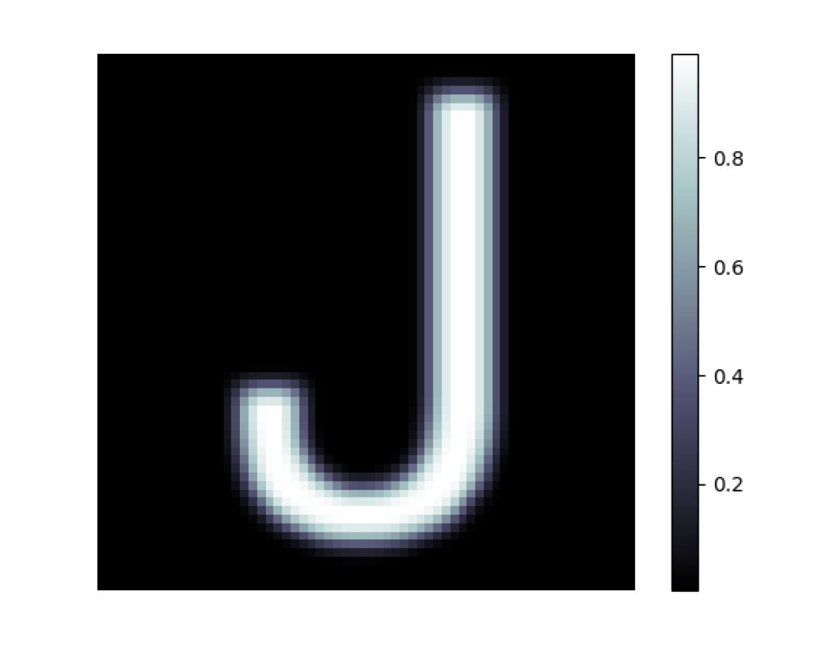
Template

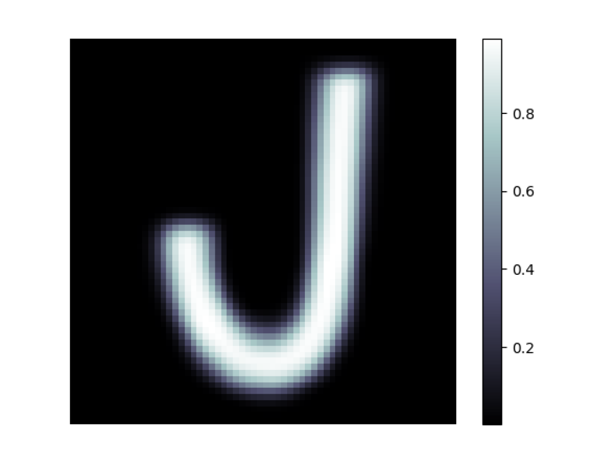
$t=0.25$

$t=0.5$

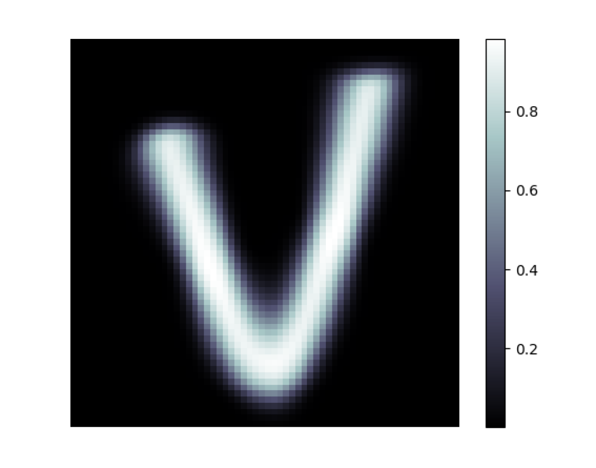
$t=0.75$

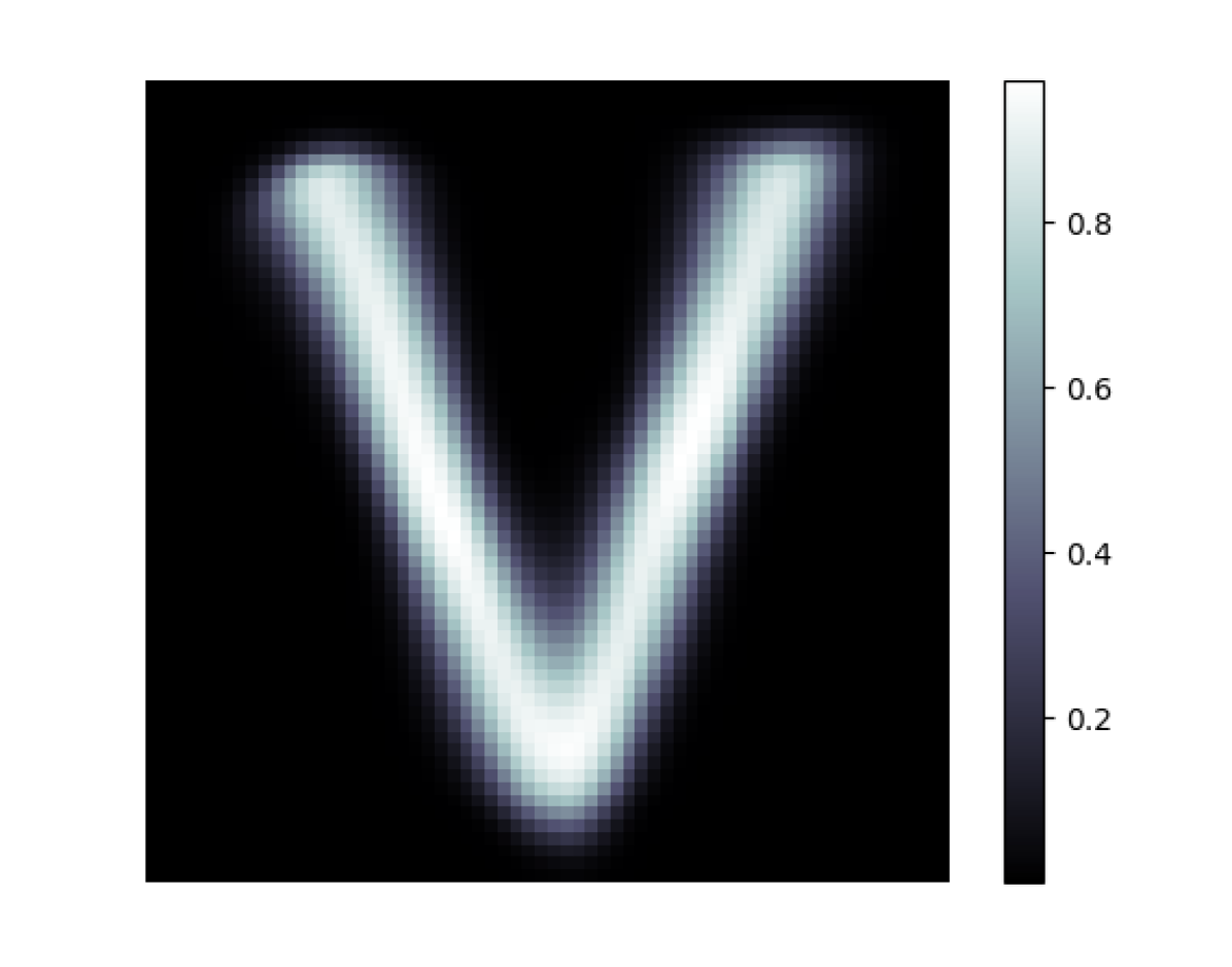
$t=1.0$

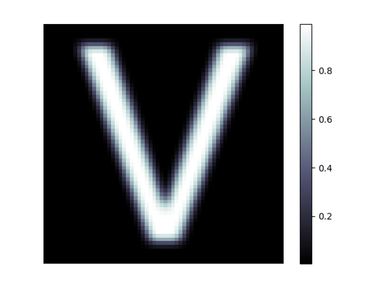
Target

Data at $0^{\circ}$

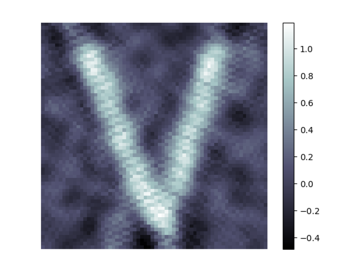
FBP

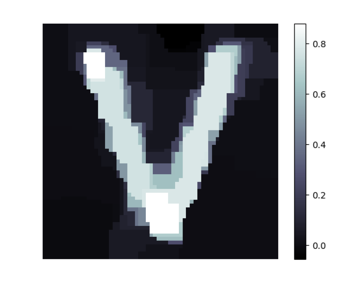
TV

Figure 1: Test suite 1: Single-object indirect registration. The template (top left) is deformed by a diffeomorphism to match the target (rightmost, second row). Images labeled with time $t$ show the final flow of diffeomorphic deformations obtained from indirect registration with $t=1.0$ denoting the final (indirectly) registered template. Data is highly noisy and under-sampled, bottom leftmost image shows data at angle $0^{\circ}$ (blue smooth curve is noise-free data, red jagged curve is noisy data). The FBP and TV reconstructions are for comparison.

Test suite 2: Multi-object indirect registration

The previous test used a target that only contains one single object. This test considers a multi-object target, namely a target consisting of six separately star-like objects with grey-values in $[0,1]$, which is digitized using $438\times 438$ pixels. The choice of target is similar to the direct registration test in [13].

The data is highly sparse parallel beam tomographic projections taken along only six directions that are uniformly distributed in $[0,180^{\circ}]$. At each direction, one samples the ray transform in a set of uniformly spaced $620$ parallel lines. Hence, the inverse problem in Eq. 1 amounts to reconstructing $191\,844$ unknowns from $3\,720$ linear equations. Besides being highly under-determined, data is also highly noisy with noise level (SNR) of $4.75$ dB.

As in test suite 1, the time interval $[0,1]$ for the flow of diffeomorphisms is sampled uniformly at $N=20$ time points, the gradient step size is set to $\alpha=0.04$, and the regularization parameter is $\gamma=10^{-7}$. On the other hand, the other regularization parameter regulating the width of the RKHS kernel is set as $\sigma=2.0$ and the gradient descent was stopped after $200$ iterations. Finally, comparison is against direct reconstructions from FBP (Hamming filter with frequency scaling $0.4$) and TV (1000 iterations, regularization parameter $\mu=1.0$).

The results, which are shown in Fig. 2, show that indirect registration performs fine also against a multi-object target as long as the template has the same number of objects.

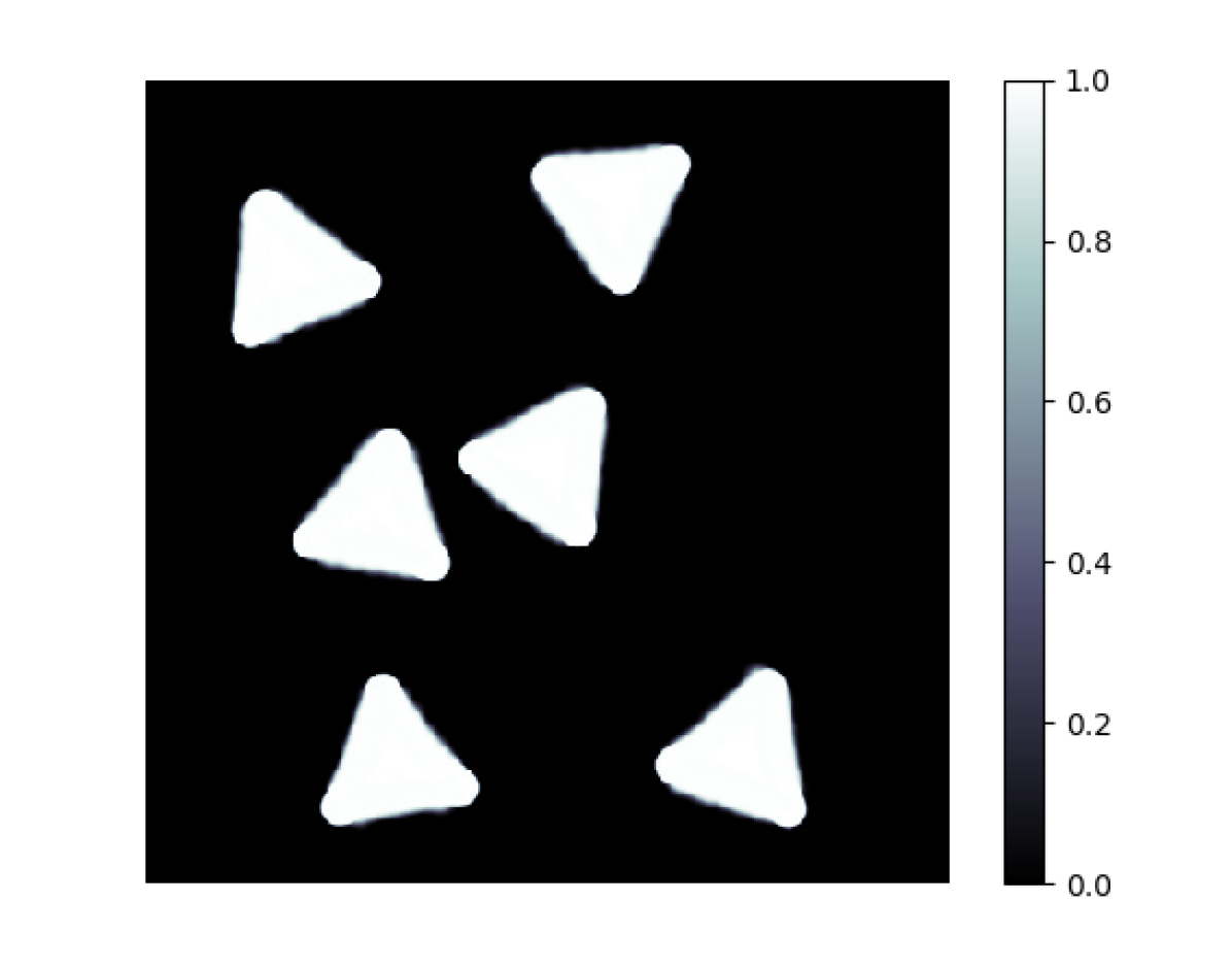
Template

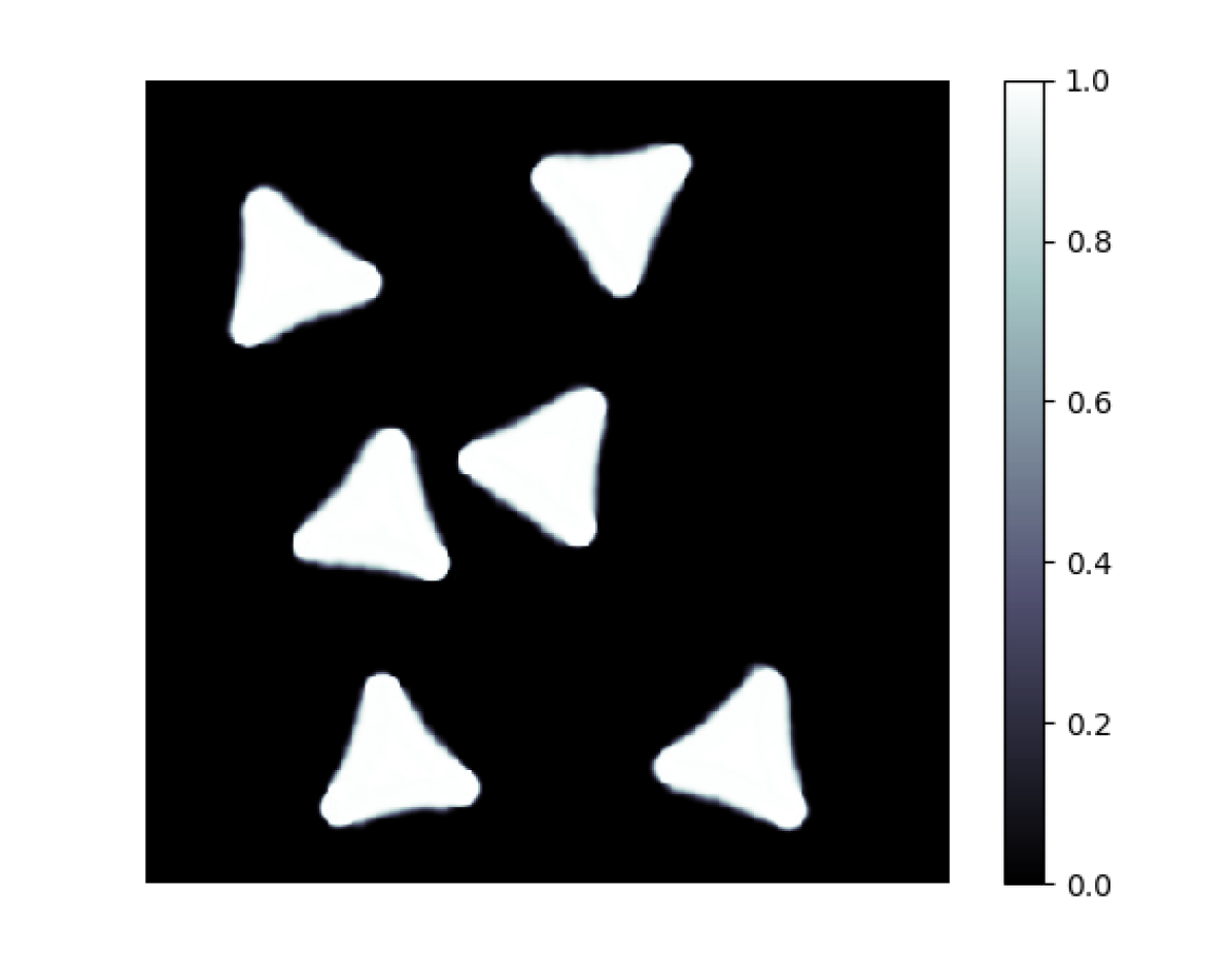
$t=0.25$

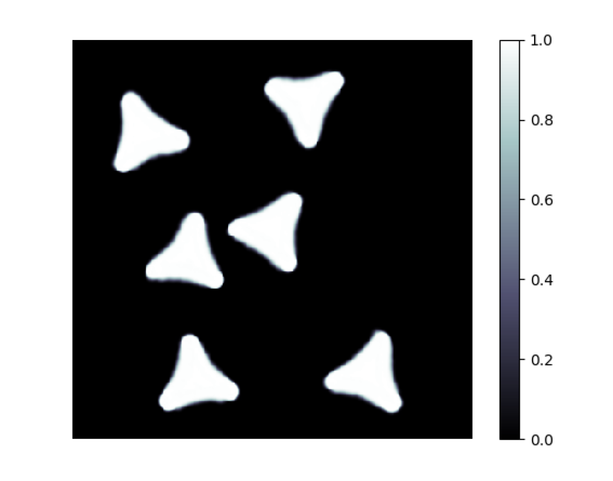
$t=0.5$

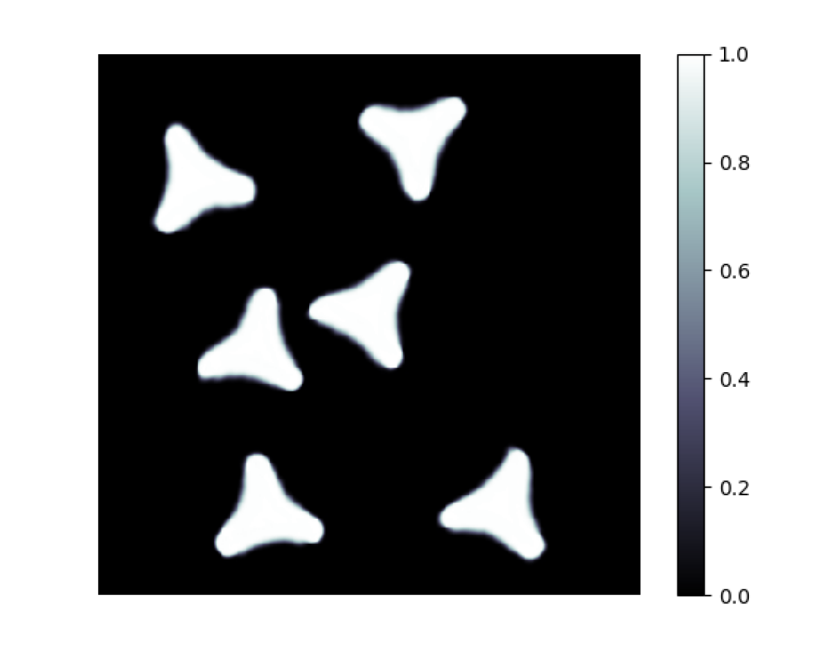
$t=0.75$

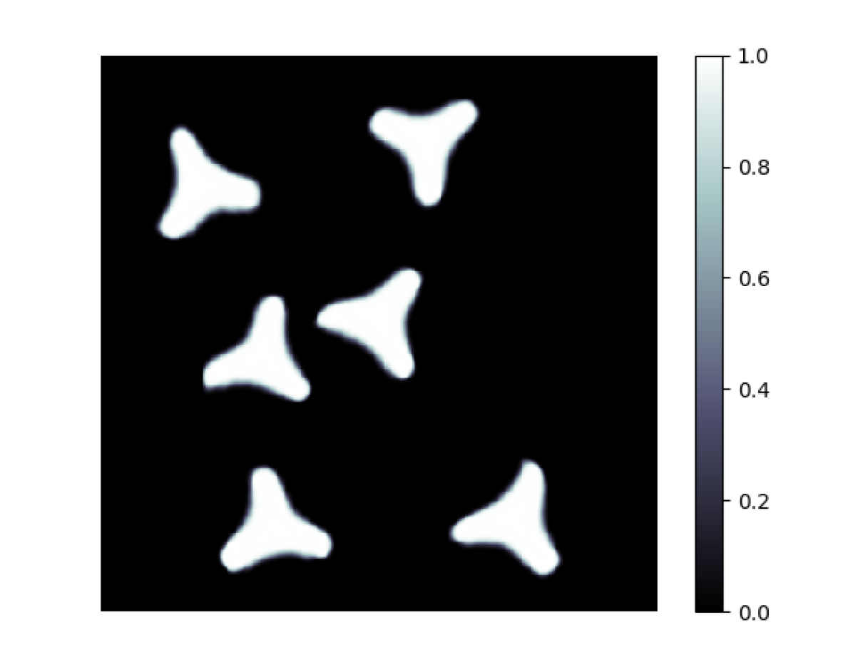
$t=1.0$

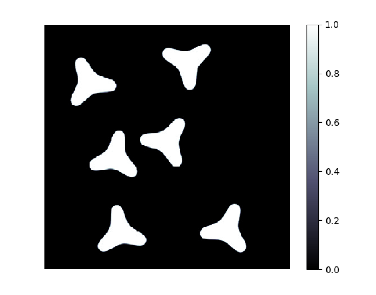
Target

Data at $0^{\circ}$

FBP

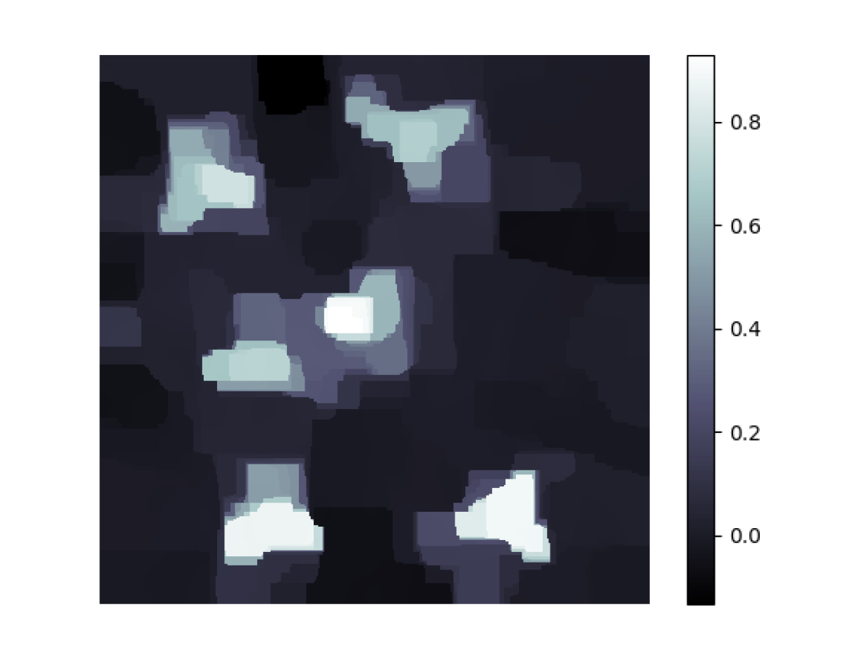
TV

Figure 2: Test suite 2: Multi-object indirect registration. The template (top left) is a target consisting of six separately triangle-like objects. Images labeled with time $t$ show the final flow of diffeomorphic deformations obtained from indirect registration with $t=1.0$ denoting the final (indirectly) registered template. Data is highly noisy and under-sampled, bottom leftmost image shows data at angle $0^{\circ}$ (blue smooth curve is noise-free data, red jagged curve is noisy data). FBP and TV reconstructions are shown for comparison.

Test suite 3: Sensitivity w.r.t. choice of regularization parameters

Choosing the regularization parameters is a well-known issue in most regularization schemes. Even though there is some theory for how to do this, in practice it is often chosen using heuristic methods and especially so when data is highly noisy and/or under-sampled. A natural question is therefore to empirically investigate the sensitivity of the indirect registration against variations in the regularization parameters $\gamma$ and $\sigma$ that enter in Eq. 83 and Eq. 84, respectively.

Here the target is the well-known Shepp-Logan phantom consisting of ten ellipsoids with grey-values in $[0,1]$. Images in shape space are digitized using $256\times 256$ pixels. The parallel beam tomographic data consists of 362 parallel line projections along ten uniformly distributed directions in $[0^{\circ},180^{\circ}]$. Hence, in a fully digitized setting, the inverse problem in Eq. 1 amounts to solving for $65\,536$ unknowns from $3\,620$ linear equations. Besides being highly under-determined, data is also highly noisy with noise level (SNR) of $7.06$ dB.

As in test suite 1, the time interval $[0,1]$ for the flow of diffeomorphism is sampled uniformly at $N=20$ time points, the gradient step size is set as $\alpha=0.02$, and the regularization parameter is $\gamma=10^{-7}$.

The regularization parameters $(\gamma,\sigma)$ are varied and each choice results in a different indirectly registered image. Each of these are then matched against the target and the registration is quantitatively assessed using SSIM [62] and PSNR [35] as figure of merits.

The SSIM and PSNR values are tabulated in Table 1, see also Fig. 3 for some selected reconstructions. As given in Table 1, the SSIM and PSNR values are quite similar for $\gamma=10^{-7},10^{-5},10^{-3},10^{-1}$ and $\sigma=1.0,2.0,2.5,3.0,4.0$. The corresponding reconstructed results in Fig. 3 are almost the same and close to the target. But these values are obviously reduced when $\gamma=10$ or $\sigma=8.0$. As shown in Fig. 3, the resulting performance is not so good compared with the target. Since the choosing intervals for $\gamma$ and $\sigma$ are relatively large, this test shows that to some extent the proposed method is not sensitive to the precise choice of the regularization parameters $\gamma$ and $\sigma$ under quantitative figures of merits (SSIM and PSNR). However those values are chosen too big that would cause over-regularized results.

	$10^{-7}$	$10^{-5}$	$10^{-3}$	$10^{-1}$	$10$
1.0	0.8958	0.8958	0.8957	0.8820	0.6800
	26.69	26.69	26.69	26.18	17.82
2.0	0.9039	0.9039	0.9038	0.8958	0.6967
	26.96	26.96	26.96	26.72	18.45
2.5	0.9018	0.9018	0.9017	0.8964	0.7057
	26.90	26.90	26.89	26.74	18.71
3.0	0.9007	0.9007	0.9006	0.8968	0.7164
	26.90	26.90	26.89	26.77	19.03
4.0	0.8992	0.8992	0.8992	0.8979	0.7426
	26.88	26.88	26.87	26.77	19.79
8.0	0.8305	0.8305	0.8307	0.8438	0.7960
	24.15	24.15	24.16	24.84	21.27

Table 1: Test suite 3: SSIM and PSNR values of indirectly registered images as compared to target for varying values of the regularization parameters $\gamma$ and $\sigma$, see Fig. 3 for selected images. Each table entry has two values, the upper is the SSIM and the bottom is the PSNR.

$\gamma=10^{-7}$, $\sigma=2.0$

$\gamma=10^{-5}$, $\sigma=2.0$

$\gamma=10^{-3}$, $\sigma=2.0$

$\gamma=10^{-7}$, $\sigma=3.0$

$\gamma=10^{-5}$, $\sigma=3.0$

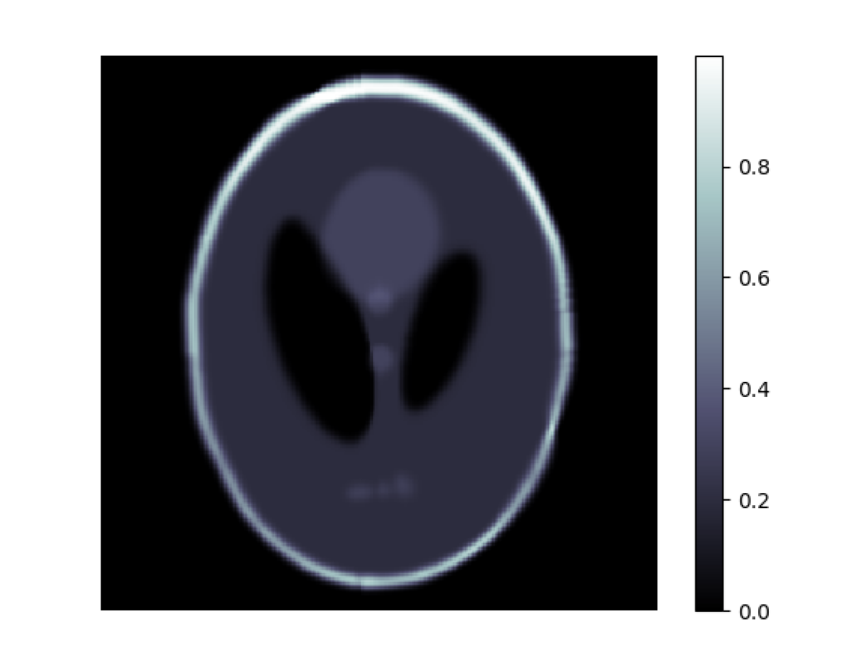
$\gamma=10^{-3}$, $\sigma=3.0$

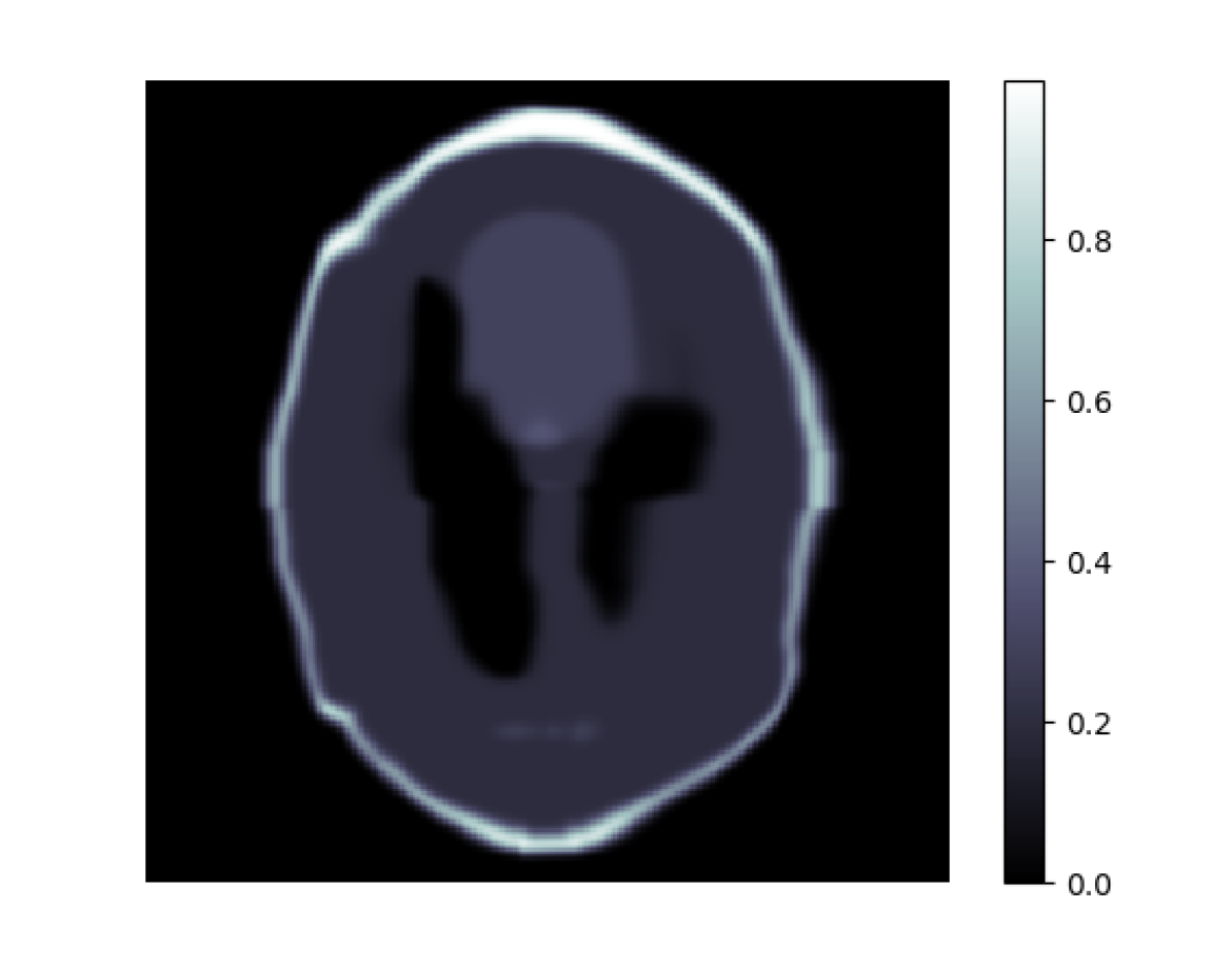
$\gamma=10^{-7}$, $\sigma=8.0$

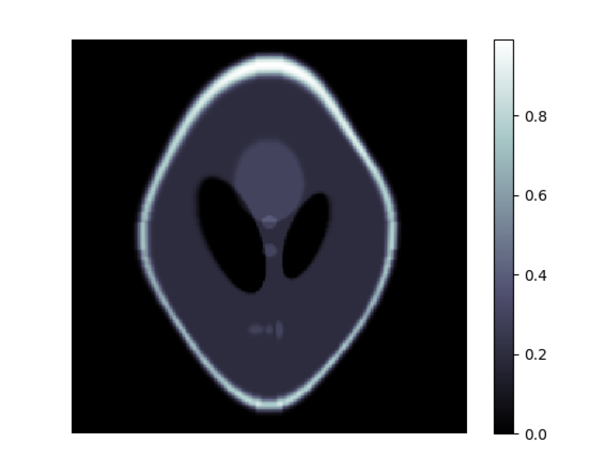
$\gamma=10.0$, $\sigma=3.0$

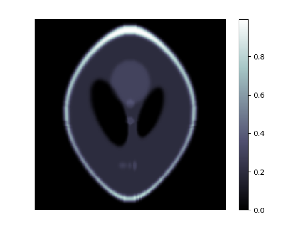
$\gamma=10.0$, $\sigma=8.0$

Template

Target

Figure 3: Test suite 3: Sensitivity w.r.t. choice of regularization parameters $\gamma$ and $\sigma$. Images show final registered result (i.e., $t=1$) for different values of these parameters. See Table 1 for a more quantitative comparison that includes a wider range of parameter values.

Test suite 4: Topology of the template

This test investigates the influence of a template with a topology that differs from the target. The test suite involves two tests, one where the the template lacks an object when compared to the target and the other where there is an additional object in the template that does not exist in the target.

In both cases, the template and the target are modifications of the Shepp-Logan phantom used in test suite 3 and tomographic data is generated following the same protocol as in test suite 3, albeit with slightly differing noise levels (7.06 dB and 6.46 dB, respectively). Finally, apart from the number of iterations which here is 1000, indirect registration in both cases was performed using the same parameter setting as in test suite 3.

Results are shown in Fig. 4. It is clear that the final indirectly registered template retains the same topology, which is to be expected since diffeomorphic registration using geometric group action can never introduce or remove an object that is not in the template. This also points to the importance of having a template with the correct topology when using diffeomorphic (indirect) registration with a geometric group action.

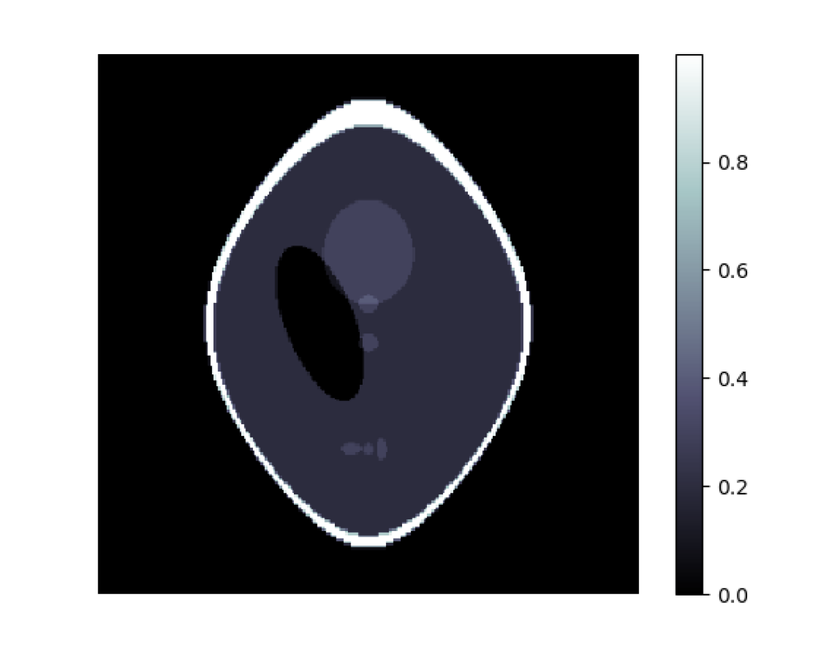
Template

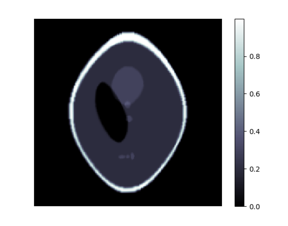
$t=0.25$

$t=0.50$

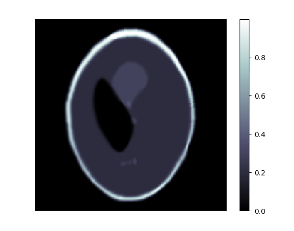
$t=0.75$

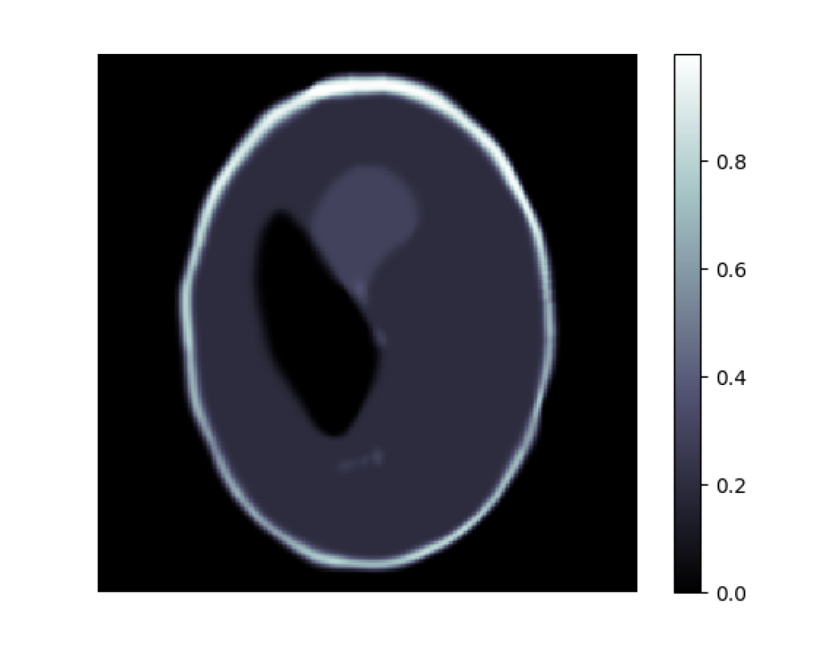
$t=1.0$

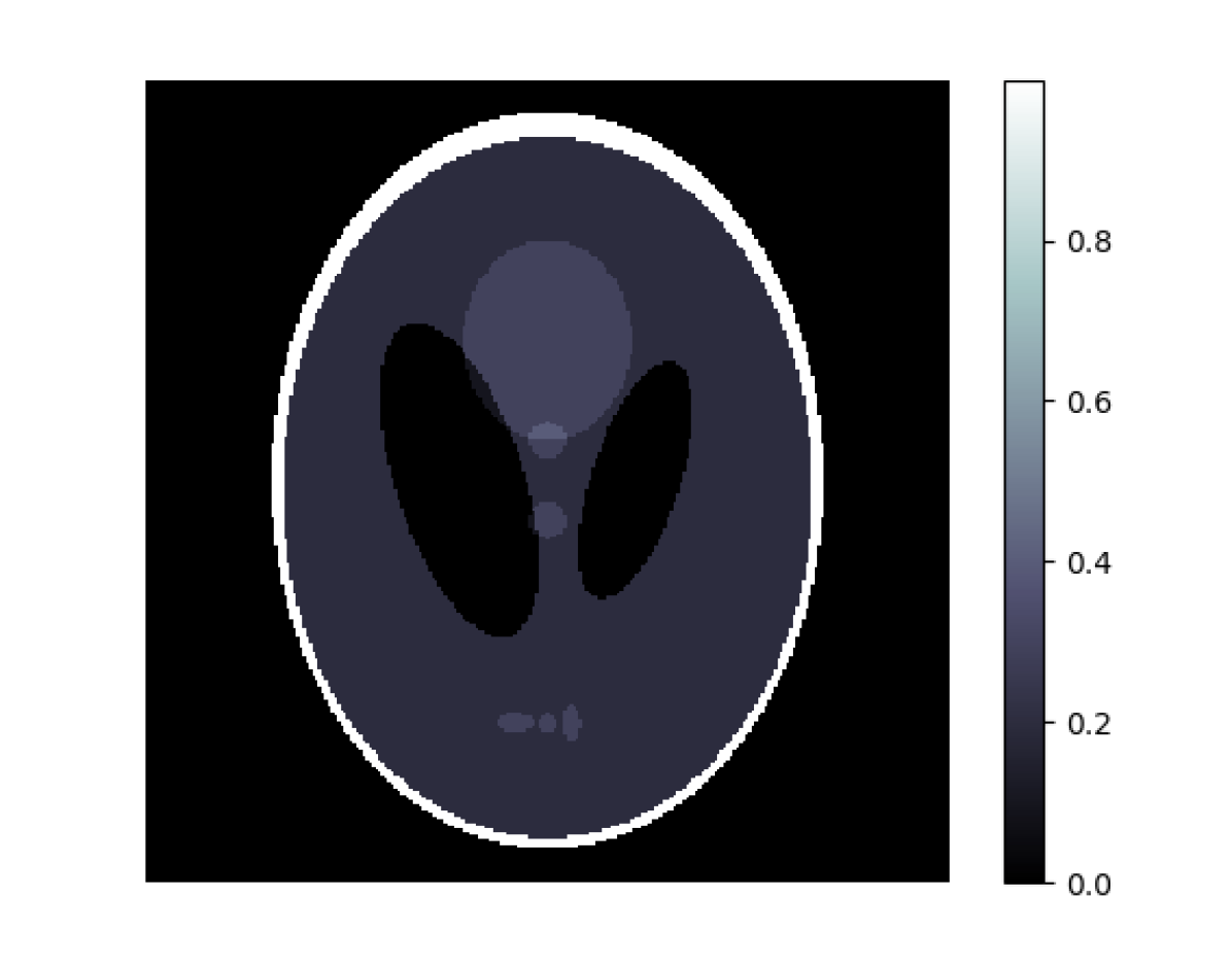
Target

Template

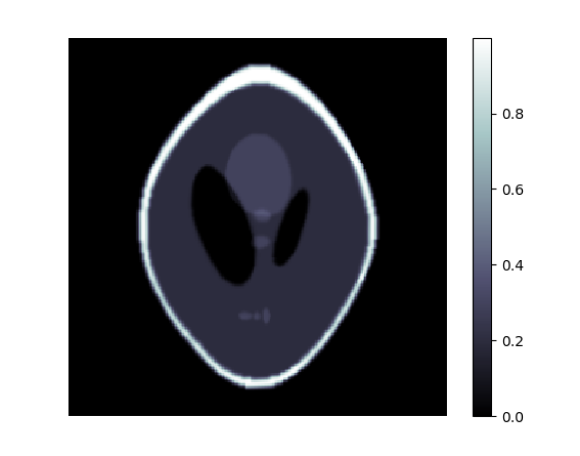
$t=0.25$

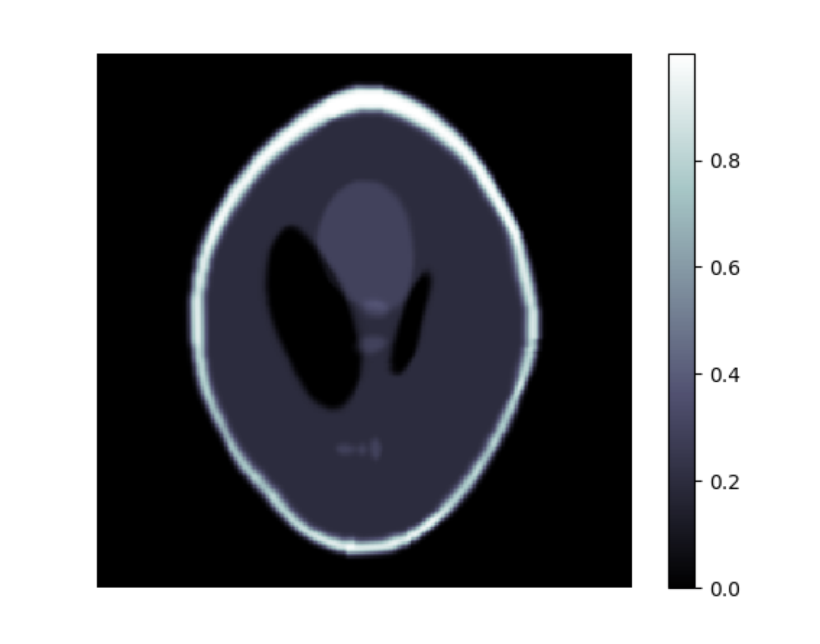
$t=0.50$

$t=0.75$

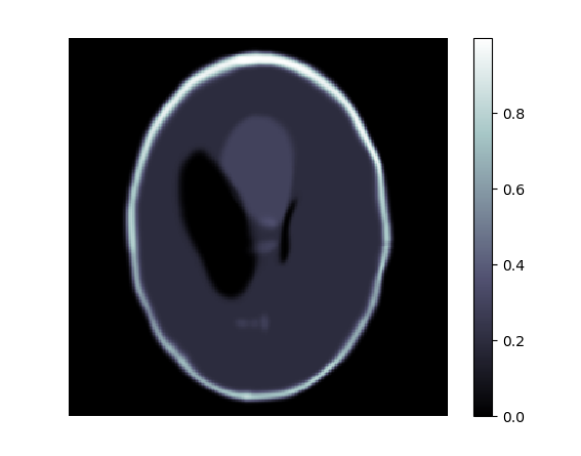
$t=1.0$

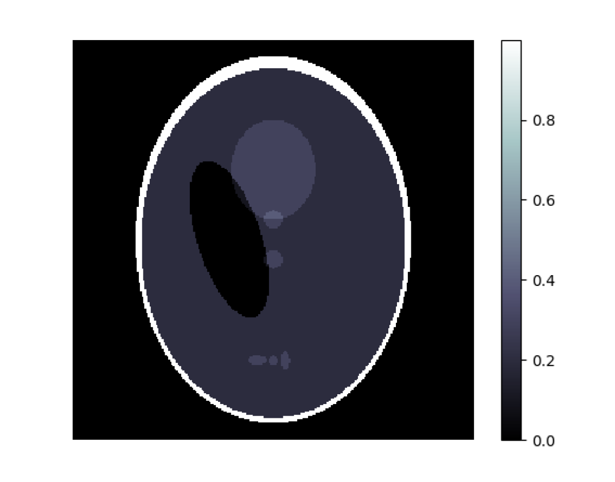
Target

Figure 4: Test suite 4: Topology of the template. First two rows is the case when the template lacks one object as compared to target, the two following rows is the case when template has one extra object. Images labeled with time $t$ show the final flow of diffeomorphic deformations obtained from indirect registration with $t=1.0$ denoting the final (indirectly) registered template.

11 Discussion

11.1 Topology and manifold structure on groups of diffeomorphisms

The LDDMM framework can be seen as part of an even more abstract formulation as outlined in [16] that involves replacing the group of diffeomorphisms in Eq. 12 with an abstract Lie group $G$ of transformations that acts on the shape space $X$, and the vector space $V$ is the corresponding Lie algebra of $G$. The situation becomes intricate when one seeks to introduce a useful manifold structure on $G$ in the infinite dimensional setting as outlined in [8].

As an example, $\operatorname{Diff}^{1}(\Omega)$ and $\operatorname{Diff}^{\infty}(\Omega)$ are both Fréchet–Lie groups, but neither is a Banach manifold. As nicely summarized in [15], working with such deformation groups allows using methods from geometry, but less tools from analysis are applicable. The other choice is to consider a group like $\operatorname{Diff}^{p}(\Omega)$. This group is a Banach manifold and a topological group so there are powerful tools from analysis for prove existence results. On the other hand, it is not a Lie group since the group operations are continuous, but not differentiable. Hence, many of the tools from differential geometry are not available.

One may next consider groups generated as in Eq. 12 from an admissible Hilbert space of vector fields. The class of admissible vector spaces is however very large, which in turn limits how far one can develop a theory for image registration in this setting. As nicely outlined in [17, p. 1538], $G_{V}$ in Eq. 12 does not need to have a differentiable structure in the general setting. Furthermore, it does not have be a topological group under the topology induced by the metric in Eq. 13. In fact, there is no natural way to define a topology on $G_{V}$ in the general setting that makes it a topological group. Hence, one has studied specific classes of admissible spaces. On the other hand, restricting attention to velocity fields with Sobolev regularity generate classical groups of Sobolev diffeomorphisms. Such a group is a Hilbert manifold as well as a topological group, but it is not necessarily a Lie group [17, p. 1512 and Theorem 8.3] but the exponential map (Remark 5.4) is continuous [17, Theorem 4.4].

11.2 Alternative frameworks for large deformations

LDDMM is capable of generating a vast range of diffeomorphic deformations, but it comes with some drawbacks coupled to its non-parametric nature. There is currently no natural parametrisation of deformations using variables that are easy to interpret from an image registration point-of-view. Furthermore, representing these non-parametric diffeomorphic deformations in software in a computationally feasible way is challenging and requires introducing further structure. This need for further structure on the group of diffeomorphic deformations has resulted in a number of parametric frameworks, some of which are mentioned below. See the excellent introduction in [33, p. 30-35] for a more informative survey.

The poly-affine framework [6, 5] considers deformations obtained by integrating trajectories of vector fields that include local affine deformations. The weights for the each local affine transformation and corresponding regions for its action remain fixed during the integration of the flow. The approach is successfully used for registration of bones [56] and images with cardiac motion [41], but the approach is not suitable for very large deformations. In the GRID model [32, 48] the idea is to fuse local deformations by fusing corresponding velocity fields. The local deformations can be more generic than in the poly-affine case, but each small deformation is located around a point (seed) that defines a local region for its action. The global deformation is a discrete temporal integration of a trajectory of corresponding vector fields. The framework has been used to model biological growth [32]. The diffeons framework [66] considers deformations are defined as the solution of a flow equation that integrates the identity map along a trajectory of vector fields. The difference to LDDMM is that one only considers trajectories of vector fields that can be written as a finite linear combination of a finite family of vector fields, called diffeons, which form a finite dimensional subspace. A further development of diffeons is deformation modules [33]. Here, one introduces a new deformation model that can generate diffeomorphisms that can be locally constrained to a certain type of deformations with a natural interpretation. The diffeomorphisms are as in LDDMM defined as final values of a flows of trajectories of vector fields and the constraints corresponds to setting of a family generators of vector fields similar to the diffeons framework.

In these parametrised frameworks, the trajectory of the vector field is constrained to be a combination of a few generators. Hence, by choosing these generators it should in principle be possible to build trajectories of diffeomorphisms that correspond to specific a priori deformations. It is however very difficult, if not impossible, to define generators that correspond to more complex deformations that typically arise in many imaging applications. Another issue that is important for image registration is to have a metric on the shape space. Another aspect relevant for (indirect) image registration is to let the metric on the group of deformations induce a metric on the shape space in a canonical manner. This is a key feature of LDDMM and it also holds for the diffeons framework, whereas this is not possible within the polyaffine and GRID frameworks.

A final recent development is to construct diffeomorphisms by using techniques from machine learning. Assume one has training data $\{(I_{i},f_{i})\}_{i}\subset X\times X$ where $f_{i}=\mathcal{W}(I_{i},\phi_{i})$ for some (unknown) deformation $\phi_{i}\in G_{V}$ and $\mathcal{W}$ given by Eq. 15. One may then use principles from machine learning to learn how to estimate the deformations from training data. The papers [63, 64] implements such as scheme. More precisely, they use machine learning in order to learn how to estimate the optimal diffeomorphic deformations. The idea is to learn the initial momenta from the training data. Once these initial momenta are learned, one can use the shooting method from LDDMM theory to generating the smallest diffeomorphic deformation [65, Section 11.6.4]. The learning is done by using a (deep) convolution neural network that learns an operator $\Lambda_{\Theta}\colon X\times X\to G_{V}$ whose parameters $\Theta$ are obtained by minimising the mean absolute error. The trained parameter yields the initial momenta, so it is now possible to generate elements in $G_{V}$ by means of the shooting method. The approach extends readily to the indirect registration setting. Training data is now $\{(I_{i},g_{i})\}_{i}\subset X\times Y$ where Eq. 18 holds, i.e., $g_{i}=\mathcal{T}\bigl{(}\mathcal{W}(I_{i},\phi_{i})\bigr{)}$ for some (unknown) deformation $\phi_{i}\in G_{V}$. One can then perform learning using a loss function similar to the direct matching case. This time the learning is done by using a (deep) convolution neural network that learns an operator $\Lambda_{\Theta}\colon X\times Y\to G_{V}$ whose parameters $\Theta$ are obtained by minimising a natural distance notion in data space. Such an approach is possible especially when combined with [1] for reconstruction.

11.3 Spatiotemporal image reconstruction

The goal here is to recover time dependent images $f_{t}\in X$ from time dependent data $g_{t}\in Y$ where $g_{t}=\mathcal{T}(f_{t})+\Delta g_{t}$ with $\Delta g_{t}$ denoting the noise term. A spatiotemporal analogue of Eq. 18 is to assume that $f_{t}=\mathcal{W}\bigl{(}\phi^{\boldsymbol{\nu}}_{0,t},I\bigr{)}$ for some unknown curve $t\mapsto\phi^{\boldsymbol{\nu}}_{0,t}$ in $G_{V}$. This allows one to formulate the following variational approach to the spatiotemporal image reconstruction problem:

(86) $$\inf_{\begin{subarray}{c}\boldsymbol{\nu}\in\mathscr{L}^{2}([0,1],V)\\ I\in X\end{subarray}}\Biggl{[}\int_{0}^{1}\biggl{(}\gamma\int_{0}^{t}\bigl{\|}\boldsymbol{\nu}(s,\cdot)\bigr{\|}^{2}_{V}\,\text{d}s+\mathcal{L}\circ\mathcal{W}\bigl{(}\phi^{\boldsymbol{\nu}}_{0,t},I\bigr{)}\biggr{)}\,\text{d}t\Biggr{]}.$$

In the above, $I\in X$ is the starting image. The curve of diffeomorphism $t\mapsto\phi^{\boldsymbol{\nu}}_{0,t}$ is generated by the velocity field $\boldsymbol{\nu}$ as a solution to Eq. 10, $\mathcal{W}\colon G_{V}\times X\to X$ is given by the group action, and $\mathcal{L}\colon X\to\mathbb{R}$ is the spatiotemporal analogue of Eq. 23, i.e.,

$$\mathcal{L}(f):=\mu\mathcal{R}(f)+\mathcal{D}\bigl{(}\mathcal{T}(f),g_{t}\bigr{)}\quad\text{for $f\in X$.}$$

The optimization problem in Eq. 86 is quite challenging and a natural approach is to consider an intertwined scheme where a reconstruction (of the template) step is followed by an indirect registration step, see [46, section 12.3] for further details. In such case, indirect registration becomes a key element in spatiotemporal image reconstruction.

11.4 Shape based reconstruction

It is possible to view indirect registration as a variational reconstruction scheme that makes use of a priori shape information encoded by the template. The tests in Section 10 indicate that if the template has the correct topology, then indirect registration performs fairly well. Furthermore, it is also robust against choice of template and regularization parameters.

When using geometric group action, indirect registration is mostly useful as a reconstruction scheme in imaging problems where the aim is to recover the shape, so intensity variations are of little, or no, importance. One example of such an imaging problem in applications is when ET is used to image the internal 3D structures at nano-scale of a specimen [13]. This is however a rather limited category of inverse problems and many of the medical imaging applications do not fall under this category. One approach to address this is to consider mass-preserving group action instead of the geometric one. Another is to keep the geometric group action, but let it act on the intensity map. This leads to metamorphosis that is briefly described in Section 11.5.

11.5 Metamorphosis

The LDDMM approach with geometric deformations only moves intensities, it does not change them. Metamorphosis extends LDDMM by allowing the diffeomorphisms to also act on intensities. This is achieved by coupling the flow equation in (10) to a similar flow equation for the intensities.

More precisely, in metamorphosis one needs to consider time dependent images. Hence, introduce $\mathscr{X}$ as the set of time dependent images that are square integrable in time and contained in $X$ at all time points. Hence, if $\zeta\in\mathscr{X}$ then $\zeta(t,\,\cdot\,)\in X$ and

$$\|\zeta\|_{\mathscr{X}}:=\sqrt{\int_{0}^{1}\bigl{\|}\zeta(t,\,\cdot\,)\bigr{\|}_{X}^{2}\,\text{d}t}<\infty.$$

The Hilbert space structure of $X$ induces a Hilbert space structures on $\mathscr{X}$. Furthermore, introduce $I\colon[0,1]\times\Omega\to\mathbb{R}$ as the solution to

(87) $$\begin{cases}\dfrac{d}{dt}I(t,x)=\zeta\bigl{(}t,\phi(t,x)\bigr{)}\quad(t,x)\in[0,1]\times\Omega,&\\[5.0pt] I(0,x)=I(x)\quad x\in\Omega.&\end{cases}$$

In the above, $\phi$ is the diffeomorphism that solves (10), $I\in X$ is the template, and $\zeta\in\mathscr{X}$ is a “source” term that is contained in the space $\mathscr{X}$ of time dependent images introduced above.

Bearing in mind the above, metamorphosis based image registration in [49] easily extends to the indirect setting, which in turn extends the LDDMM based indirect registration in Eq. 24:

(88) $$\begin{cases}\displaystyle{\inf_{\begin{subarray}{c}\boldsymbol{\nu}\in\mathscr{L}^{2}([0,1],V)\\ \zeta\in\mathscr{X}\end{subarray}}}\Bigl{[}\gamma\|\boldsymbol{\nu}\|_{\mathscr{L}^{2}([0,1],V)}^{2}+\tau\|\zeta\|_{\mathscr{X}}^{2}+\mathcal{L}\circ\mathcal{V}\bigl{(}\boldsymbol{\nu},I(1,\,\cdot\,)\bigr{)}\Bigr{]}&\\[20.00003pt] \dfrac{d}{dt}I(t,x)=\zeta\bigl{(}t,\phi^{\boldsymbol{\nu}}_{0,t}(x)\bigr{)}\quad(t,x)\in[0,1]\times\Omega,&\\[5.0pt] I(0,x)=I(x)\quad x\in\Omega.\end{cases}$$

Here, $\mathcal{L}\colon X\to\mathbb{R}$ is given by Eq. 23 and $\mathcal{V}\colon\mathscr{L}^{2}([0,1],V)\times X\to X$ is given by Eq. 45 (geometric group action). Note that the velocity field $\boldsymbol{\nu}\in\mathscr{L}^{2}([0,1],V)$ in the objective also generates, through Eq. 10, the diffeomorphism $\phi^{\boldsymbol{\nu}}_{0,t}\colon\Omega\to\Omega$ in the ODE constraint. Furthermore, $I(1,\,\cdot\,)\in X$ in the objective functional depends on the optimization variable $\zeta\in\mathscr{X}$ through the ODE constraint. Finally, as in Section 6.1.1 for LDDMM, one can re-phrased (88) as a PDE constrained problem:

(89) $$\begin{cases}\displaystyle{\inf_{\begin{subarray}{c}\boldsymbol{\nu}\in\mathscr{L}^{2}([0,1],V)\\ \zeta\in\mathscr{X}\end{subarray}}}\Big{[}\gamma\|\boldsymbol{\nu}\|_{\mathscr{L}^{2}([0,1],V)}^{2}+\tau\|\zeta\|_{\mathscr{X}}^{2}+\mathcal{L}\bigl{(}f(1,\,\cdot\,)\bigr{)}\Bigr{]}&\\[10.00002pt] \partial_{t}f(t,x)+\Bigl{\langle}\nabla_{x}f(t,x),\boldsymbol{\nu}(t,x)\Bigr{\rangle}_{\mathbb{R}^{n}}\!\!=\zeta(t,x)\quad(t,x)\in[0,1]\times\Omega,&\\[5.0pt] f(0,x)=I(x)\quad x\in\Omega.\end{cases}$$

11.6 Relation to optimal transport

Optimal transport is a well developed mathematical theory that defines a family of metrics between probability distributions. These metrics measure the mass of an optimal displacement according to a base cost defined on the space supporting the distributions. Wasserstein distance refers to using $\mathscr{L}^{p}$-norm as base costs. It is a deep mathematical theory [61] with many applications. Applications to imaging is nicely surveyed in [47], the focus here is on its usage in diffeomorphic image registration.

Optimal transport metrics are suitable for shape registration since they are sensitive to spatial displacements of the shape. This framework is [20, 37] extended to handle measures of different total mass (unbalanced optimal transport), which makes it applicable to a wider range of image registration problems. Another aspect associated with using optimal transport distances is computability. Without approximations, it is computationally feasible only for 1D images. This situation has however changed during the last few years, much due to using entropic approximation schemes resulting in Sinkhorn-type iterations [23]. Such an approach is developed in [36] for indirect image registration where the authors used Sinkhorn-type iterations to compute the proximal operator of the transport problem for large problems, such as indirect image registration in tomography. This scheme also applies to unbalanced optimal transport in [29] to quantify the similarity in diffeomorphic registration of imaging data. Finally, [40] combines metamorphosis with optimal transport for image registration. The numerical method is based on adding a transport penalty to the objective in Eq. 89, which is the PDE constrained formulation of metamorphosis.

References

- [1] J. Adler and O. Öktem, Learned primal-dual reconstruction, E-print math.OC 1707.06474, ArXiv e-prints, 2017. Accepted for publication in IEEE Transactions on Medical Imaging.
- [2] L. Ambrosio, Transport equation and Cauchy problem for BV vector fields, Inventiones Mathematicae, 158 (2004), pp. 227—260.
- [3] L. Ambrosio and E. De Giorgi, New functionals in the calculus of variations, Atti della Accademia Nazionale dei Lincei: Rendiconti Lincei - Matematica e Applicazioni, 82:8 (1988), pp. 199—210.
- [4] N. Aronszajn, Theory of reproducing kernels, Transactions of the American Mathematical Society, 68 (1950), pp. 337–404.
- [5] V. Arsigny, O. Commowick, N. Ayache, and X. Pennec, A fast and log-Euclidean polyaffine framework for locally linear registration, Journal of Mathematical Imaging and Vision, 33 (2009), pp. 222—238.
- [6] V. Arsigny, X. Pennec, and N. Ayache, Polyrigid and polyaffine transformations: a novel geometrical tool to deal with non-rigid deformations–application to the registration of histological slices, Medical image analysis, 9 (2005), pp. 507—523.
- [7] A. I. Awad and M. Hassaballah, eds., Image Feature Detectors and Descriptors: Foundations and Applications, vol. 630 of Studies in Computational Intelligence, Springer-Verlag, 2016.
- [8] A. Banyaga, The Structure of Classical Diffeomorphism Groups, Kluwer, 1997.
- [9] M. Bauer, S. Joshi, and K. Modin, Diffeomorphic density matching by optimal information transport, SIAM Journal on Imaging Sciences, 8 (2015), pp. 1718–1751.
- [10] F. Becker, S. Petra, and C. Schnörr, Optical flow, in Handbook of Mathematical Methods in Imaging, O. Scherzer, ed., Springer-Verlag, 2nd ed., 2015, pp. 1945–2004.
- [11] F. M. Beg, M. I. Miller, A. Trouvé, and L. Younes, Computing large deformation metric mappings via geodesic flow of diffeomorphisms, International Journal of Computer Vision, 61 (2005), pp. 139—157.
- [12] A. Berlinet and C. Thomas-Agnan, Reproducing Kernel Hilbert Spaces in Probability and Statisties, Springer-Verlag, 2004.
- [13] E. Bladt, D. M. Pelt, S. Bals, and K. J. Batenburg, Electron tomography based on highly limited data using a neural network reconstruction technique, Ultramicroscopy, 158 (2015), pp. 81–88.
- [14] F. Bonin-Font, A. Ortiz, and G. Oliver, Visual navigation for mobile robots: A survey, Journal of Intelligent and Robotic Systems, 53 (2008), pp. 263–296.
- [15] M. Bruveris, Notes on Riemannian geometry on manifolds of maps. Lecture notes for IMS Summer School on Mathematics of Shapes, 4–15 July 2016. Available online from http://www2.ims.nus.edu.sg/Programs/016shape/files/martins.pdf, 2016.
- [16] M. Bruveris and D. D. Holm, Geometry of image registration: The diffeomorphism group and momentum maps, in Geometry, Mechanics, and Dynamics: The Legacy of Jerry Marsden, C. D. E., D. D. Holm, G. Patrick, and T. Ratiu, eds., vol. 73 of Fields Institute Communications, Springer-Verlag, 2015, pp. 19–56.
- [17] M. Bruveris and F.-X. Vialard, On completeness of groups of diffeomorphisms, Journal of the European Mathematical Society, 19 (2017), pp. 1507–1544.
- [18] M. Burger and S. Osher, A guide to the TV zoo, in Level Set and PDE Based Reconstruction Methods in Imaging, M. Burger and S. Osher, eds., vol. 2090 of Lecture Notes in Mathematics, Springer-Verlag, 2013, pp. 1–70.
- [19] A. Chambolle and T. Pock, A first-order primal-dual algorithm for convex problems with applications to imaging, Journal of Mathematical Imaging and Vision, 40 (2011), pp. 120–145.
- [20] L. Chizat, B. Schmitzer, G. Peyré, and F.-X. Vialard, An interpolating distance between optimal transport and Fisher-Rao, Foundations of Computational Mathematics, (2016).
- [21] G. E. Christensen, R. D. Rabbitt, and M. I. Miller, Deformable template model using large deformation kinematics, IEEE Transactions on Image Processing, 5 (1996), pp. 1435–1447.
- [22] M. Colombo, Flows of Non-smooth Vector Fields and Degenerate Elliptic Equations with Applications to the Vlasov-Poisson and Semigeostrophic Systems, Publications of the Scuola Normale Superiore, Springer-Verlag, 2017.
- [23] M. Cuturi, Sinkhorn distances: Lightspeed computation of optimal transportation, in Proceedings of NIPS, vol. 26, 2013, pp. 2292—2300.
- [24] T. D’Arcy, On Growth and Form, Cambridge University Press, New York, 1945.
- [25] S. Dawn, V. Saxena, and B. Sharma, Remote sensing image registration techniques: A survey, in Image and Signal Processing. Proceedings of the 4th International Conference, ICISP 2010, Trois-Rivières, QC, Canada, June 30-July 2, 2010, A. Elmoataz, O. Lezoray, F. Nouboud, D. Mammass, and J. Meunier, eds., vol. 6134 of Lecture Notes in Computer Science, 2010, pp. 103–112.
- [26] E. De Giorgi and L. Ambrosio, New functionals in calculus of variations, in Nonsmooth Optimization and Related Topics, F. H. Clarke, V. F. Dem’yanov, and F. Giannessi, eds., vol. 43 of Part of the Ettore Majorana International Science Series book series (EMISS), Springer-Verlag, 1989, ch. 4, pp. 49–59.
- [27] C. Demant, B. Streicher-Abel, and C. Garnica, Industrial Image Processing: Visual Quality Control in Manufacturing, Springer-Verlag, 2013.
- [28] R. J. DiPerna and P.-L. Lions, Ordinary differential equations, transport theory and Sobolev spaces, Inventiones Mathematicae, 98 (1989), pp. 511—547.
- [29] J. Feydy, B. Charlier, F.-X. Vialard, and G. Peyré, Optimal transport for diffeomorphic registration, E-print math.NA 1706.05218, ArXiv e-prints, 2017.
- [30] M. Grasmair, Generalized Bregman distances and convergence rates for non-convex regularization methods, Inverse Problems, 26 (2010), p. 115014.
- [31] U. Grenander and M. I. Miller, Pattern Theory. From Representation to Inference, Oxford University Press, 2007.
- [32] U. Grenander, A. Srivastava, and A. Saini, A pattern-theoretic characterization of biological growth, IEEE Transactions on Medical Imaging, 26 (2007), pp. 648—659.
- [33] B. Gris, Modular approach on shape spaces, sub-Riemannian geometry and computational anatomy, PhD thesis, École Normale Supérieure de Paris-Saclay, 2016.
- [34] Y. Hong, S. Joshi, M. Sanchez, M. Styner, and M. Niethammer, Metamorphic geodesic regression, in Medical Image Computing and Computer-Assisted Intervention – MICCAI 2012 15th International Conference, Nice, France, October 1-5, 2012, Proceedings, Part II, N. Ayache, P. Delingette, H. Golland, and K. Mori, eds., vol. 7512 of Lecture Notes in Computer Science, Springer-Verlag, 2012, pp. 197–205.
- [35] Q. Huynh-Thu and M. Ghanbari, Scope of validity of PSNR in image/video quality assessment, Electronics Letters, 44 (2008), pp. 800–801.
- [36] J. Karlsson and A. Ringh, Generalized sinkhorn iterations for regularizing inverse problems using optimal mass transport, E-print math.OC 1612.02273, ArXiv e-prints, 2016. Accepted for publication in SIAM Journal on Imaging Sciences.
- [37] M. Liero, A. Mielke, and G. Savaré, Optimal entropy-transport problems and a new Hellinger-Kantorovich distance between positive measures, E-print math.OC 1508.07941, ArXiv e-prints, 2016.
- [38] T. Lindeberg, Generalized axiomatic scale-space theory, Advances in Imaging and Electron Physics, 178 (2013), pp. 1–96.
- [39] T. Lindeberg, Image matching using generalized scale-space interest points, Journal of Mathematical Imaging and Vision, 52 (2015), pp. 3–36.
- [40] J. Maas, M. Rumpf, C. Schönlieb, and S. Simon, A generalized model for optimal transport of images including dissipation and density modulation, ESAIM: Mathematical Modelling and Numerical Analysis, 49 (2015), pp. 1745–1769.
- [41] K. McLeod, M. Sermesant, P. Beerbaum, and X. Pennec, Spatio-temporal tensor decomposition of a polyaffine motion model for a better analysis of pathological left ventricular dynamics, IEEE Transactions on Medical Imaging, 34 (2015), pp. 1562—1575.
- [42] M. Micheli and J. A. Glaunès, Matrix-valued kernels for shape deformation analysis, Geometry, Imaging, and Computing, 1 (2013), pp. 57–139.
- [43] M. I. Miller, A. Trouvé, and L. Younes, Hamiltonian systems and optimal control in computational anatomy: 100 years since D’Arcy Thompson, Annual Review of Biomedical Engineering, 17 (2015), pp. 447–509.
- [44] K. P. Murphy, Machine Learning: A Probabilistic Perspective, MIT Press, Cambridge, MA, USA, 2012.
- [45] F. Natterer and F. Wübbeling, Mathematical Methods in Image Reconstruction, Mathematical Modeling and Computation, Society for Industrial and Applied Mathematics, 2001, http://epubs.siam.org/doi/book/10.1137/1.9780898718324.
- [46] O. Öktem, C. Chen, N. O. Domaniç, P. Ravikumar, and C. Bajaj, Shape based image reconstruction using linearised deformations, Inverse Problems, 33 (2017), p. 035004.
- [47] N. Papadakis, Optimal transport for image processing, hal id: tel-01246096, Université de Bordeaux, 2016. Avaialble from https://hal.archives-ouvertes.fr/tel-01246096v6.
- [48] N. Portman and E. R. Vrscay, Existence and uniqueness of solutions to the grid macroscopic growth equation, Applied Mathematics and Computation, 217 (2011), pp. 8318—8327.
- [49] C. L. Richardson and L. Younes, Metamorphosis of images in reproducing kernel Hilbert spaces, Advances in Computational Mathematics, 42 (2016), pp. 573—603.
- [50] W. Ring and B. Wirth, Optimization methods on Riemannian manifolds and their application to shape space, SIAM Journal of Optimization, 22 (2012), pp. 596–627.
- [51] E. Sariyanidi, H. Güneş, and A. Cavallaro, Automatic analysis of facial affect: A survey of registration, representation, and recognition, IEEE Transactions on Pattern Analysis and Machine Intelligence, 37 (2015), pp. 1113–1133.
- [52] O. Scherzer, M. Grasmair, H. Grossauer, M. Haltmeier, and F. Lenzen, Variational Methods in Imaging, vol. 167 of Applied Mathematical Sciences, Springer-Verlag, New York, 2009.
- [53] J. A. Schnabel, M. P. Heinrich, B. W. Papieżc, and M. J. Brady, Advances and challenges in deformable image registration: From image fusion to complex motion modelling, Medical Image Analysis, 33 (2016), pp. 145–148.
- [54] B. Scholkopf and A. J. Smola, Learning with Kernels: Support Vector Machines, Regularization, Optimization, and Beyond, MIT Press, Cambridge, MA, USA, 2001.
- [55] L. Schwartz, Sous-espaces Hilbertiens d’espaces vectoriels topologiques et noyaux associés (noyaux reproduisants), Journal d’Analyse Mathématique, 13 (1964), pp. 115–256.
- [56] C. Seiler, X. Pennec, and M. Reyes, Capturing the multi-scale anatomical shape variability with polyaffine transformation trees, Medical image analysis, 16 (2012), pp. 1371—1384.
- [57] A. Sotiras, C. Davatzikos, and N. Paragios, Deformable medical image registration: A survey, IEEE Transactions on Medical Imaging, 32 (2013), pp. 1153–1190.
- [58] A. Trouvé and L. Younes, Shape spaces, in Handbook of Mathematical Methods in Imaging, S. Otmar, ed., Springer-Verlag, 2011, ch. 30, pp. 1309–1362.
- [59] F.-X. Vialard, Hamiltonian Approach to Shape Spaces in a Diffeomorphic Framework: From the Discontinuous Image Matching Problem to a Stochastic Growth Model, PhD thesis, École normale supérieure de Cachan, Centre de Mathématiques et de Leurs Applications, 61, avenue du Président Wilson, Cachan, 2009.
- [60] M. A. Viergever, J. B. Maintz, S. Klein, K. Murphy, M. Staring, and J. P. Pluim, A survey of medical image registration, Medical Image Analysis, 33 (2016), pp. 140–144.
- [61] C. Villani, Optimal Transport: Old and New, Grundlehren der mathematischen Wissenschaften, Springer-Verlag, 2009.
- [62] Z. Wang, A. C. Bovik, H. R. Sheikh, and E. P. Simoncelli, Image quality assessment: from error visibility to structural similarity, IEEE Transactions on Image Processing, 13 (2004), pp. 600–612.
- [63] X. Yang, R. Kwitt, and M. Niethammer, Fast predictive image registration, in Deep Learning and Data Labeling for Medical Applications: Proceedings of the First International Workshop (LABELS 2016) and Second International Workshop (DLMIA 2016) Held in Conjunction with MICCAI 2016, G. Carneiro, D. Mateus, L. Peter, A. Bradley, J. M. R. S. Tavares, V. Belagiannis, J. P. Papa, J. C. Nascimento, M. Loog, Z. Lu, J. S. Cardoso, and J. Cornebise, eds., vol. 10008 of Lecture Notes in Computer Science, 2016, pp. 48–47.
- [64] X. Yang, R. Kwitt, M. Styner, and M. Niethammer, Quicksilver: Fast predictive image registration – a deep learning approach, NeuroImage, 158 (2017), pp. 378–396.
- [65] L. Younes, Shapes and Diffeomorphisms, vol. 171 of Applied Mathematical Sciences, Springer-Verlag, 2010.
- [66] L. Younes, Constrained diffeomorphic shape evolution, Foundations of Computational Mathematics, 12 (2012), pp. 295—325.
- [67] B. Zitová and J. Flusser, Image registration methods: a survey, Image and Vision Computing, 21 (2003), pp. 977–1000.