Migration and kinematics in growing disc galaxies with thin and thick discs

Abstract

We analyse disc heating and radial migration in $N$-body models of growing disc galaxies with thick and thin discs. Similar to thin-disc-only models, galaxies with appropriate non-axisymmetric structures reproduce observational constraints on radial disc heating in and migration to the Solar Neighbourhood (Snhd). The presence of thick discs can suppress non-axisymmetries and thus higher baryonic-to-dark matter fractions are required than in models that only have a thin disc. Models that are baryon-dominated to roughly the Solar radius $R_{0}$ are favoured, in agreement with data for the Milky Way. For inside-out growing discs, today’s thick-disc stars at $R_{0}$ are dominated by outwards migrators. Whether outwards migrators are vertically hotter than non-migrators depends on the radial gradient of the thick disc vertical velocity dispersion. There is an effective upper boundary in angular momentum that thick disc stars born in the centre of a galaxy can reach by migration, which explains the fading of the high $\left[{\rm\alpha/Fe}\right]$ sequence outside $R_{0}$. Our models compare well to Snhd kinematics from RAVE-TGAS. For such comparisons it is important to take into account the azimuthal variation of kinematics at $R\sim R_{0}$ and biases from survey selection functions. The vertical heating of thin disc stars by giant molecular clouds is only mildly affected by the presence of thick discs. Our models predict higher vertical velocity dispersions for the oldest stars than found in the Snhd age velocity dispersion relation, possibly because of measurement uncertainties or an underestimation of the number of old cold stars in our models.

1 Introduction

Gilmore & Reid (1983) discovered that the vertical star count density in the Milky Way (MW) near the Sun could be fitted by a double-exponential profile. The two components have become known as the thin disc and the thick disc. Jurić et al. (2008) find scaleheights of $h_{z,{\rm thin}}=300\,{\rm pc}$ and $h_{z,{\rm thick}}=900\,{\rm pc}$ and a local thick disc contribution to the stellar surface density of $\sim 26$ per cent. The majority of edge-on disc galaxies in the local Universe prove to have vertical surface brightness profiles that are consistent with a similar double-exponential structure (Comerón et al., 2011).

The thick part of the density profile is made up of stellar populations with hotter vertical kinematics, which in comparison to the thin populations, have a different chemical composition in the form of enhanced $\alpha$-element abundances relative to their iron content, $\left[{\rm\alpha/Fe}\right]$ (Fuhrmann, 1998), and older ages (Masseron & Gilmore, 2015). High $\left[{\rm\alpha/Fe}\right]$ populations have been found to be more centrally concentrated than thin disc stars (Bensby et al., 2011; Cheng et al., 2012) and to fade outside a Galactic radius of $R\sim 10\,{\rm kpc}$ (Hayden et al., 2015). Radial age gradients at high altitudes $|z|>1\,{\rm kpc}$ (Martig et al., 2016) suggest that chemical and geometrical definitions of the thick disc can yield very different results in the outer Galaxy. The formation scenarios for thick discs split mainly into two groups: (i) the heating of an initially thin disc in galaxy mergers (e.g. Quinn et al., 1993), or (ii) the birth of thick disc stars on kinematically hot orbits (e.g. Bird et al., 2013). For (ii) both the formation in an early gas-rich and turbulent phase dominated by mergers and high gas accretion rates (Brook et al., 2004) and the continuous decrease of birth velocity dispersions of stars in discs with declining gas fractions and turbulence driven by gravitational disc instabilities (Forbes et al., 2012) have been suggested.

The diverse chemical compositions of stars in the Solar Neighbourhood (Snhd) favour models in which Snhd stars were born at a variety of Galactic radii. The chemical pattern in thick-disc stars requires that these stars originated in significantly more central regions than the Snhd (Schönrich & Binney, 2009a) and that the Galaxy has undergone an inside-out formation scenario (Schönrich & McMillan, 2017). The high $\alpha$ abundances at high iron abundance $\left[{\rm Fe/H}\right]$ of some thick-disc stars require very high star formation efficiencies in the early MW (Andrews et al., 2017) and thus a compact star-forming disc.

The process that has been identified as responsible for spreading stars away from their birth radii is radial migration. It happens when stars are scattered by a non-axisymmetric structure such as a bar or a spiral arm across the structure’s corotation resonance, which leads to their angular momentum changing appreciably without significantly increasing random motions (Sellwood & Binney, 2002). It can explain the chemical diversity of Snhd stars (Schönrich & Binney, 2009a, b) and the dependence of the specific shape of stellar metallicity distribution on Galactic radius (Loebman et al., 2016).

Schönrich & Binney (2009b) and Schönrich & McMillan (2017) showed that in their analytical Galaxy models, which couple dynamics and chemical evolution, radial migration is responsible for the formation of the thick disc as outwards migrating stars from hot inner disc parts provide a population of vertically hot stars at outer radii. The source of vertical heating in the inner disc was left unspecified in this work, which assumed that the velocity dispersions of a stellar population are specified by its birth radius and age through a combination of: (i) an inwards increasing vertical velocity dispersion, that would ensure a radially constant scaleheight in the absence of radial migration, and (ii) a radially independent time dependence of the vertical heating law $\sigma_{z}(t)$. Whereas Schönrich & Binney (2009b) assumed that during migration the energy of vertical oscillations is conserved, Schönrich & McMillan (2017) corrected this assumption to conservation of vertical action (Solway et al., 2012).

Simulations of disc galaxies forming from the cooling of rotating hot gas haloes have roughly confirmed this picture (Loebman et al., 2011; Roškar et al., 2013) and studies of radial migration in thick and thin disc systems found mildly lower but significant levels of migration in the thick populations (Solway et al., 2012). However, several other studies have cast doubt on the migration origin of the thick disc (Minchev et al., 2012; Vera-Ciro et al., 2014, 2016), as they concluded that vertically hot stars are less prone to radial migration than vertically cool stars.

Important observational constraints on the evolution of the MW come from the age velocity dispersion relation (AVR), which shows that bluer and therefore younger populations have lower velocity dispersions in all three directions $R$, $\phi$ and $z$ than redder, older populations (Parenago, 1950; Wielen, 1977; Dehnen & Binney, 1998; Holmberg et al., 2009). Interestingly, if one uses stars close to the Sun from the Geneva Copenhagen Survey (GCS, Nordström et al., 2004; Casagrande et al., 2011), the oldest stars show vertical velocity dispersions $\sigma_{z}\sim 30\,{\rm km\,s^{-1}}$. This is significantly lower than the $\sigma_{z}\sim 40-50\,{\rm km\,s^{-1}}$ found for high $\left[{\rm\alpha/Fe}\right]$ stars by Bovy et al. (2012a). Moreover, the vertical AVR shows no step in time, as might be expected from a merger scenario, and as had been claimed to have been found in the Snhd (Quillen & Garnett, 2001).

In Aumer et al. (2016a) (hereafter Paper 1), we presented a set of $\sim 100$ $N$-body simulations of disc galaxies growing within live dark matter (DM) haloes over $\sim 10\,{\rm Gyr}$. In Aumer et al. (2016b) (hereafter Paper 2), we analysed the stellar kinematics of these models to get a better understanding on disc heating in MW-like disc galaxies. Papers 1 and 2 established that giant molecular clouds (GMCs) are a necessary ingredient for reproducing disc structure and kinematics as they are the main vertical heating agent for the thin disc and can explain the vertical thin-disc AVR in the Snhd. Moreover, we showed that models which combined the standard values for dark-halo mass and baryonic Galaxy mass could reproduce the radial AVR and the amount of migration required to explain the chemistry of the Snhd. Because both quantities are determined by non-axisymmetric disc structures, we can assume that they were appropriately captured by the models.

As none of these models contains a thick disc similar to that in the MW, Aumer & Binney (2017) (hereafter Paper 3) introduced a new set of simulations in which thick discs were either present in the initial conditions (ICs) or created by adding stars on orbits with continuously decreasing velocity dispersions. Paper 3 showed that several of these models are capable of simultaneously roughly reproducing for the MW the vertical and radial mass distributions, the length and edge-on profile of the bar, vertical and radial age gradients of disc stars and constraints on the DM density in the Snhd and the circular-speed curve.

Here we use a subset of the simulations from Papers 1 and 3 to study radial migration and Snhd kinematics in models with thin and thick discs. We clarify the extent to which the presence of a thick disc modifies our conclusions regarding disc heating and migration, and we quantify migration of thick-disc stars. We use the models to investigate the impact of the Galactic bar and spiral structure on measurements of disc kinematics such as those recently released by the Gaia consortium (Gaia Collaboration, 2016b).

The paper is structured as follows. Section 2 summarises the setup and parameters of the simulations and can be skipped by a reader familiar with Paper 3. Section 3 quantifies the radial migration by stars of various ages. Section 4 compares the stellar kinematics extracted from our models with data from the MW: Section 4.1 analyses velocity distributions in the $R$, $\phi$, and $z$ directions and compares them to recent data from RAVE and TGAS; Section 4.2 discusses how well AVRs of models with thin and thick discs compare to Snhd data. In Section 5 we discuss our results with an emphasis on the role of radial migration in the formation of the chemically-defined thick disc (Section 5.1) and on how disc heating shapes Snhd kinematics (Section 5.2). Section 6 sums up.

Table 1: List of models analysed in this paper and their parameters. 1st Column: Model Name; 2nd Column: Initial Conditions; 3rd Column: Initial baryonic mass $M_{\rm b,i}$; 4th Column: Concentration parameter for IC dark halo $c_{\rm halo}$; 5th Column: IC scalelength $h_{\rm IC}$; 6th Column: IC disc scaleheight $z_{0,{\rm disc}}$; 7th Column: Total inserted baryonic model mass $M_{\rm f}$ (including initial baryonic mass); 8th Column: Final time $t_{\rm f}$; 9th Column: Initial disc scalelength $h_{R,{\rm i}}$; 10th Column: Final disc scalelength $h_{R,{\rm f}}$; 11th Column: Scalelength growth parameter $\xi$; 12th Column: Stellar exponential scalelength $h_{R}(R_{0},t_{\rm f})$ determined from all stars within $5.8<R/\,{\rm kpc}<10.8$ at $t_{\rm f}$ ; 13th Column: Type of SFR law; 14th Column: Exponential decay timescale $t_{\rm SFR}$ for the star formation rate; 15th Column: Radial to vertical dispersion ratio for inserted particles $\lambda$; 16th Column: Prescription for initial velocity dispersion for inserted stellar particles, $\sigma_{0}(t)$; 17th-18th Column: Parameters $\sigma_{1}$ and $t_{1}$, which determine $\sigma_{0}(t)$; 19th Column: GMC star formation efficiency $\zeta$.

1st	2nd	3rd	4th	5th	6th	7th	8th	9th	10th	11th	12th	13th	14th	15th	16th	17th	18th	19th
Name	ICs	$M_{\rm b,i}$	$c_{\rm halo}$	$h_{\rm IC}$	$z_{0,{\rm disc}}$	$M_{\rm f}$	$t_{\rm f}$	$h_{R,{\rm i}}$	$h_{R,{\rm f}}$	$\xi$	$h_{R}(R_{0},t_{\rm f})$	SF Type	$t_{\rm SFR}$	$\lambda$	$\sigma_{0}$	$\sigma_{1}$	$t_{1}$	$\zeta$
		$[10^{9}\,M_{\odot}]$		$[\,{\rm kpc}]$	$[\,{\rm kpc}]$	$[10^{10}\,M_{\odot}]$	$[\,{\rm Gyr}]$	$[\,{\rm kpc}]$	$[\,{\rm kpc}]$		$[\,{\rm kpc}]$		$[\,{\rm Gyr}]$		Type	$[\,{\rm km\,s^{-1}}]$	$[\,{\rm Gyr}]$
Y1	Y	5	9.0	1.5	0.10	5	10	1.5	4.3	0.5	4.0	1	8.0	1.0	const	6	–	0.08
P1s6	P	15	9.0	2.5	1.75	5	10	1.5	4.3	0.5	2.8	0	–	1.0	const	6	–	0.08
P2	P	15	9.0	2.5	1.75	5	10	2.5	2.5	0.0	3.0	1	8.0	1.0	const	6	–	0.08
Q1$\zeta$-	Q	25	6.5	2.5	1.75	6	10	1.5	4.3	0.5	4.1	1	8.0	1.0	const	6	–	0.04
U1	U	25	7.5	2.0	1.70	6	10	1.5	4.3	0.5	5.8	1	8.0	1.0	const	6	–	0.08
M$\alpha$1	M	5	9.0	1.5	–	5	10	1.5	4.3	0.5	3.2	1	8.0	1.0	atan	16	2.0	0.08
M$\beta$1s5	M	5	9.0	1.5	–	5	12	1.5	4.3	0.5	2.8	1	8.0	1.0	plaw	51	1.57	0.08
V$\alpha$8s7	V	5	6.5	1.5	–	6	12	1.0	4.3	0.6	3.7	2	12.0	1.0	atan	16	3.5	0.08
V$\beta$8s5	V	5	6.5	1.5	–	6	12	1.0	4.3	0.6	5.6	1	8.0	1.0	plaw	51	1.57	0.08
V$\alpha$9s8$\lambda\zeta$*	V	5	6.5	1.5	–	6	12	1.0	3.5	0.6	3.1	1	6.0	1.25	atan	16	2.0	0.06

2 Simulations

Table 1 lists the small subset of the simulations presented in Papers 1 and 3 that are discussed in this paper. We discuss only collisionless simulations of growing disc galaxies within non-growing live dark haloes made using the Tree code gadget-3, last described in Springel (2005). We distinguish between (i) thin-disc-only simulations (Y1), (ii) models with thick discs in their ICs (P, Q and U models), and (iii) models in which stars are added with continuously declining velocity dispersions (declining $\sigma_{0}$ models with V and M ICs).

A model is specified by the initial conditions from which it starts and the rules used to feed in stars. For a full account of the meaning of all parameters and the model names we refer to Papers 1 and 3. Here we only give a brief overview. In the Appendix A, we present figures which show basic structural properties for each of the models studied in this paper.

We focus on standard-resolution models, which at the end of the simulation contain $N_{\rm b}=5-6\times 10^{6}$ stellar particles with particle masses $m_{\rm b}=10^{4}\,M_{\odot}$ and $N_{\rm DM}=5\times 10^{6}$ DM particles with masses $m_{\rm DM}=2\times 10^{5}\,M_{\odot}$. In addition, the simulations contain a population of short-lived, massive particles representing GMCs with masses $m_{\rm GMC}=10^{5-7}\,M_{\odot}$ following a GMC mass function similar to that observed in the MW. The force softening lengths are $\epsilon_{\rm b}=30\,{\rm pc}$ for baryonic particles (including GMCs) and $\epsilon_{\rm DM}=134\,{\rm pc}$ for DM particles.

2.1 Initial conditions

Table 1 of Paper 3 lists the details of the ICs, which were created using the galic code (Yurin & Springel, 2014). All models discussed here start with a spherical dark halo with a Hernquist (1990) profile

$$\rho_{\rm{DM}}(r)={{M_{\rm{DM}}}\over{2\pi}}{{a}\over{r\left(r+a\right)^{3}}}.$$ (1)

and mass $M_{\rm DM}=10^{12}\,M_{\odot}$. The inner density profiles are adjusted to be similar to NFW profiles with concentration parameters in the range $c_{\rm halo}=6-9$.

The ICs contain either a stellar disc (Y, P, Q or U ICs) or a low-density distorted stellar bulge resembling a rotating elliptical galaxy (M and V ICs). IC discs have a mass profile

$${\rho_{\rm{disc,i}}(R,z)}={{M_{\rm{b,i}}}\over{4\pi{z_{0,{\rm disc}}}{h_{\rm IC}}^{2}}}{\operatorname{sech}^{2}\left({z}\over{z_{0,{\rm disc}}}\right)}{\exp\left(-{R}/{h_{\rm IC}}\right)}.$$ (2)

Here $h_{\rm IC}$ is the IC disc exponential scalelength and a radially constant isothermal vertical profile with scaleheight $z_{0,{\rm disc}}$ is assumed. The Y model starts with a baryonic disc of mass $M_{\rm b,i}=5\times 10^{9}\,M_{\odot}$, which is compact ($h_{\rm IC}=1.5\,{\rm kpc}$) and thin ($z_{0,{\rm disc}}=0.1\,{\rm kpc}$), whereas the P, Q and U models contain a much thicker, more extended and more massive IC disc ($z_{0,{\rm disc}}\sim 1.7\,{\rm kpc}$, $h_{\rm IC}=2.0-2.5\,{\rm kpc}$, $M_{\rm b,i}=15-25\times 10^{9}\,M_{\odot}$).

The baryonic ICs of the M and V models have a Hernquist profile with $M_{\rm b,i}=5\times 10^{9}\,M_{\odot}$ and $a=h_{\rm IC}=1.5\,{\rm kpc}$. The mass profile is distorted to an oblate spheroid with axis ratio $s=2$ as $\rho_{\rm elliptical}(R,z)=s\rho_{\rm Hernquist}\Bigl{(}\sqrt{R^{2}+s^{2}z^{2}}\Bigr{)}$.

2.2 Growing the discs

Stellar particles are continuously added to the disc following a star formation rate ${\rm SFR}(t)$ that is either constant in time (type 0), declines exponentially as

$${\rm SFR}(t)={\rm SFR}_{0}\times\exp({-t/t_{\rm SFR}})\,\,\,{\rm{(type\,1)}},$$ (3)

or has an additional early increase

$${\rm SFR}(t)={\rm SFR}_{0}\times\exp({-t/t_{\rm SFR}}-{0.5\,{\rm Gyr}/t})\,\,\,{\rm{(type\,2)}},$$ (4)

with $t_{\rm SFR}=6-12\,{\rm Gyr}$. The constant ${\rm SFR}_{0}$ is adjusted to produce at $t=t_{\rm f}$ a target final baryonic mass $M_{\rm f}$ in the range $5-6\times 10^{10}\,M_{\odot}$ including the IC mass $M_{\rm b,i}$.

As was discussed in Papers 1 and 3, mass growth and the influence of bars and spirals change the surface density profiles of stars of all ages and lead to final profiles which differ from simple exponentials. To characterise the total final stellar surface density profile $\Sigma(R)$ in a Snhd-like location, we fit an exponential to $\Sigma(R)$ at $t_{\rm f}$ in the region $5.8<R/\,{\rm kpc}<10.8$ centred around $R_{0}=8.3\,{\rm kpc}$ and give the resulting scalelength $h_{R}(R_{0},t_{\rm f})$ in Table 1. We note that not all of the profiles are well-fitted by exponentials in this radial range.

Every five Myr, stellar particles are added at $z=0$ and randomly chosen azimuths, and with an exponential radial density profile $\Sigma_{\rm SF}(R)\propto\exp(-R/h_{R}(t))$. The scalelength $h_{R}(t)$ of the newly added particles grows in time as

$$h_{R}(t)=h_{R,\rm i}+(h_{R,\rm f}-h_{R,\rm i})(t/t_{\rm f})^{\xi}.$$ (5)

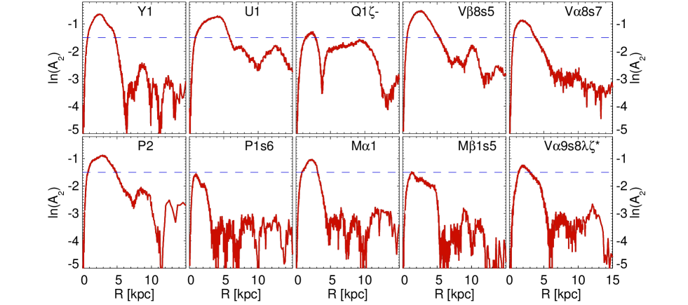
Figure 15: Radial profiles of the $m=2$ Fourier amplitude $A_{2}(R)$ measured at $t=t_{\rm f}$. The blue dashed lines mark $\ln(A_{2})=-1.5$.

To avoid inserting particles in the bar region, particles are not added inside a cutoff radius $R_{\rm cut}$, which is determined by the current bar length as measured by the $m=2$ Fourier amplitude $A_{2}(R)$. If there is a peak in $A_{2}$ with $\ln(A_{2})>-1.5$ in the inner galaxy, we set $R_{\rm cut}$ to the smaller of 5 kpc and the radius where $\ln(A_{2})(R)$ drops below $-1.5$. Our choice for the cutoff is empirical in nature and was discussed in Paper 1. We find that the upper limit for the cutoff length does not prevent longer bars from forming (e.g. in model U1) and that these longer bars are not significantly different from shorter bars. We find that our cutoff definition is reasonably well suited for the models presented here as it picks out the strong bar regions and avoids contributions from spirals (see e.g. Figure 15). We caution that this need not be the case for any possible model.

GMCs are modelled as a population of massive collisionless particles drawn from a mass function of the form ${\rm d}N/{\rm d}M\propto M^{\gamma}$ with lower and upper mass limits $M_{\rm low}=10^{5}\,M_{\odot}$ and $M_{\rm up}=10^{7}\,M_{\odot}$ and an exponent $\gamma=-1.6$. GMC particles are added in the same region, with the same profile as stellar particles and on orbits with birth velocity dispersion $\sigma_{0}=6\,{\rm km\,s^{-1}}$ (see Section 2.3). Their azimuthal density is given by

$$\rho_{\rm GMC}(\phi)\propto\left[\rho_{\rm ys}(\phi)\right]^{\alpha},$$ (6)

where $\rho_{\rm ys}$ is the density of young stars and $\alpha=1$. The mass in GMCs is determined by the SF efficiency $\zeta=0.04-0.08$. Specifically, for each $\Delta m_{\rm stars}$ of stars formed, a total GMC mass $\Delta m_{\rm GMC}=\Delta m_{\rm stars}/\zeta$ is created. GMC particles live for only $50\,{\rm Myr}$: for $25\,{\rm Myr}$ their masses grow with time as $m\propto t^{2}$, and for the final $25\,{\rm Myr}$ of their lives their masses are constant. At early times, GMCs can contain a substantial fraction of the baryonic galaxy mass, especially for models with low IC masses, low $\zeta$ and short $t_{\rm SFR}$. For model V$\alpha$9s8$\lambda\zeta$* at early times, 45 per cent of the baryonic mass is in GMCs. At late times, GMC mass fractions are low: $2-3$ per cent.

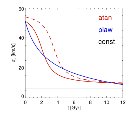
Figure 1: Evolution of input velocity parameter $\sigma_{0}$ with simulation time $t$ for various scenarios . The black line is for type ‘const’, the red lines for type ‘atan’ (dashed for $t_{1}=3.5\,{\rm Gyr}$, solid for $t_{1}=2.0\,{\rm Gyr}$) and the blue line for type ‘plaw’.

2.3 Birth velocity dispersions

The young stellar populations are assigned birth velocity dispersions $\sigma_{0}(t)$. For thin-disc-only simulations and models with thick-disc ICs we assign a constant $\sigma_{z}=\sigma_{R}=\sigma_{\phi}=\sigma_{1}=6\,{\rm km\,s^{-1}}$. The mean rotation velocity $\langle v_{\phi}\rangle(R)$ at radius $R$ is set to the circular speed $v_{\rm circ}=\sqrt{{a_{R}(R)}R}$, where $a_{R}(R)$ is the azimuthal average of the radial gravitational acceleration, $\partial\Phi/\partial R$.

For declining $\sigma_{0}$ models we use two different functional forms for $\sigma_{0}(t)$:

$$\sigma_{0}(t)=\sigma_{1}\left[{\arctan\left({t_{1}-t}\over{1\,{\rm Gyr}}\right)}+{{\pi}\over{2}}\right]+8\,{\rm km\,s^{-1}}\,\,\,{\rm(type\,atan)}$$ (7)

or

$$\sigma_{0}(t)=\sigma_{1}\left({t+t_{1}}\over{2.7\,{\rm Gyr}}\right)^{-0.47}-15\,{\rm km\,s^{-1}}\,\,\,{\rm(type\,plaw)}.$$ (8)

We assume that $\sigma_{0}$ is independent of radius $R$ and always set $\sigma_{z}=\sigma_{0}$ and $\sigma_{\phi}=\sigma_{R}/\sqrt{2}$. We test values $\sigma_{R}=\lambda\sigma_{0}$ with $\lambda=1-1.3$ and apply an asymmetric drift correction for $\langle v_{\phi}\rangle(R)$ derived from Equation (4.228) in Binney & Tremaine (2008). Figure 1 visualises the difference between assumed histories of the decline in $\sigma_{0}$. For models with declining $\sigma_{0}$ we choose a higher thin-disc input dispersion $\sigma_{0}\sim 10\,{\rm km\,s^{-1}}$ than in the models with constant $\sigma_{0}=6\,{\rm km\,s^{-1}}$. As was shown in Paper 2 this yields a somewhat better fit to Snhd AVRs. The AVRs of the present simulations are discussed in Section 4.2.

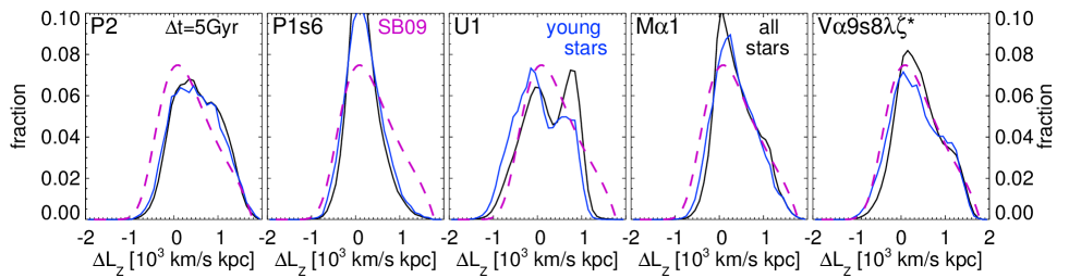
Figure 2: Plots of changes in $L_{z}$ in the last $5\,{\rm Gyr}$ for samples of stars selected to have $L_{z}=L_{z,{\rm circ}}(8\,{\rm kpc})\pm 100\,{\rm kpc}\,{\rm km\,s^{-1}}$ at $t=t_{\rm f}$ in various models. The black curves are for all stars that are more than $5\,{\rm Gyr}$ old, while the blue curves are for stars with ages $5-6\,{\rm Gyr}$, so $\Delta L_{z}$ is the change in their angular momentum since they were young. Also plotted in a broken line is the corresponding distribution inferred by Schönrich & Binney (2009a) from the chemical composition of Snhd.

3 Radial Migration

We begin the analysis of the selected models by studying radial migration of disc stars of various ages and over different timescales to gain a better understanding of how the models differ and to understand how well they fulfil constraints set by chemical evolution models, which require a significant level of radial migration to explain the variety of stellar chemical compositions found in the Snhd (Schönrich & Binney, 2009a).

3.1 Thin-disc constraints

With Figure 2 we test whether the conclusion from Paper 1, that thin-disc-only models of appropriate mass in appropriate dark haloes provide the right amount of migration to explain the chemistry of the Snhd is also true for thin disc components in thin+thick disc systems. We plot histograms of the change $\Delta L_{z}\equiv L_{z}(t_{\rm f})-L_{z}(t_{\rm f}-5\,{\rm Gyr})$ in the angular momentum of stars which at $t=t_{\rm f}$ have angular momentum in the range $L_{z}=L_{z,{\rm circ}}(8\,{\rm kpc})\pm 100\,{\rm kpc}\,{\rm km\,s^{-1}}$. Here $L_{z,{\rm circ}}\equiv Rv_{\rm circ}(R)$ and these stars thus have current guiding centre radii $R_{\rm g}\approx 8\,{\rm kpc}$. The black curves include all stars born before $t_{\rm f}-5\,{\rm Gyr}$, while the blue curves are for stars younger than $1\,{\rm Gyr}$ at that time, so $\Delta L_{z}$ is the change in their angular momentum since they were young. The pink dashed curve is from the chemical evolution model of Schönrich & Binney (2009a).

Model P2 shows, both for all stars, and just young stars, a $\Delta L_{z}$ histogram which is very similar to the one predicted for the Snhd by Schönrich & Binney (2009a). It is also similar to the histogram of Model YG1 presented in Paper 1, which demonstrates that the presence of a thick disc and the relatively late formation of a bar in P2 do not suppress migration to $R=8\,{\rm kpc}$. Model P1s6 has less non-axisymmetric structure than P2 (see Paper 3 and Figure 15), so its $\Delta L_{z}$ distribution is significantly narrower than required by Snhd chemistry.

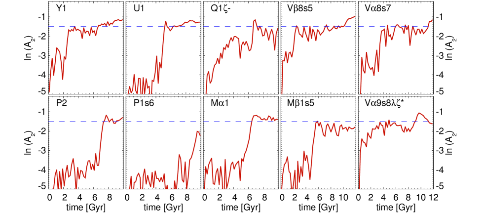
Figure 14: Evolution with time of $m=2$ Fourier amplitude $A_{2}$ measured within $R=3\,{\rm kpc}$. The blue dashed lines mark $\ln(A_{2})=-1.5$.

The histogram for Model U1 shows a sharper cutoff at high $\Delta L_{z}$. As was discussed in Paper 1, this cutoff is caused by the early presence of a relatively long bar, out of which stars cannot escape to reach radii close to $R_{0}$. Curiously, especially the old stars show a double-peaked $\Delta L_{z}$ histogram. This feature arises already between $t=5$ and $6\,{\rm Gyr}$, when it is more strongly detectable and is connected to the corotation resonance of the bar which forms at $t\sim 5\,{\rm Gyr}$ (see Figure 14).

Models M$\alpha$1 and V$\alpha$9s8$\lambda\zeta$* have declining $\sigma_{0}$. The choice of a radially constant input dispersion $\sigma_{0}$ leads to on average higher velocity dispersions at outer radii than in models with thick-disc ICs. This in turn reduces the strength of non-axisymmetric structures, as shown in Figure 15. Consequently, Model M$\alpha$1, despite having a reasonably sized bar, shows mildly too little radial migration. By contrast, V$\alpha$9s8$\lambda\zeta$*, which has a more massive and more compact disc and lives in a lower density halo, has a distribution of $\Delta L_{z}$ that comes very close to that inferred from observational data by Schönrich & Binney (2009a).

Note that the difference between all stars and young stars is not significant for any models. Given that in all models young populations are on average vertically cooler than the average over all stars, which includes the thick disc, this implies significant migration taking place for vertically hotter stars. We will examine this further below.

In light of these results, it is interesting to reconsider the results of Figure 9 of Paper 3. This figure plots the evolution of the exponential scalelengths of mono-age populations measured at a Solar-like radius $h_{R}(R_{0})$. It shows that any model that features the required amount of radial migration also shows an increase during the last $5\,{\rm Gyr}$ in $h_{R}(R_{0})$ for populations of all ages. So, the non-axisymmetries in the MW that caused radial migration likely also affected the radial surface density profiles of stars at $R_{0}$ in a flattening way.

3.2 Migration to the Snhd as a function of age

In Figure 3 we analyse the origin of all stars that at $t=t_{\rm f}$ live at $R=8\pm 0.5\,{\rm kpc}$. Note that unlike in Section 3.1 we here select stars in $R$ and not $L_{z}$. The upper row of panels shows the distribution of these stars in the plane of age $\tau$ and $\Delta L_{z}=L_{z}(t_{\rm f})-L_{z}(t_{\rm birth})$, the angular momentum change since birth. The horizontal dashed lines mark the distinction between IC stars and added stars.

We start by analysing the inside-out growing thin-disc-only model Y1. We notice that the youngest stars, which have not had enough time to migrate significantly, show a rather even distribution around $\Delta L_{z}=0$. Towards the older added and IC stars the distribution bends clearly towards positive $\Delta L_{z}$, i.e. the majority of stars were born at smaller $L_{z}$ and have migrated outwards. Y1 has a compact early disc with $h_{R}=1.5\,{\rm kpc}$ both for IC stars and the first inserted stars, which means there simply aren’t many stars at $R=8\,{\rm kpc}$ at these times. Moreover, non-axisymmetric structures are strong from relatively early on (Figure 14) and the populations are all initially cold, which leads to significant migration of these old populations over the course of the simulations.

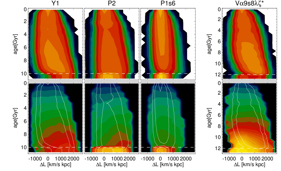
Figure 3: Upper panels: the density of stars, which at $t=t_{\rm f}$ are at $R=8\pm 0.5\,{\rm kpc}$, in the $\tau$-$\Delta L_{z}$ plane. $\tau$ is the age of a star and $\Delta L_{z}=L_{z}(t_{\rm f})-L_{z}(t_{\rm birth})$ is the change in angular momentum a star has undergone since birth. The horizontal dashed lines mark the distinction between IC stars and added stars. Lower panels: the vertical velocity dispersion $\sigma_{z}$ at $t=t_{\rm f}$ of stars at $R=8\pm 0.5\,{\rm kpc}$ in the $\tau$-$\Delta L_{z}$ plane. White contours are for density as in the upper row.

Model P2 has a thick, more extended IC disc with $h_{R}=2.5\,{\rm kpc}$ and an insertion scalelength that is constant at the same value. We see two main differences. (i) Unlike in Y1, there is a discontinuity in the $\Delta L_{z}$ distribution between the IC stars and the old inserted stars. This is because IC stars have a different original $L_{z}$ distribution and are vertically hotter than the other populations, which are all born cold and, notwithstanding GMC heating, have at all times lower $\sigma_{z}$ than the IC stars (see Section 4.2). The vertically hotter IC stars at $R\sim R_{0}$ and $t=t_{\rm f}$ have migrated less than the cooler, old inserted stars, a result similar to those of both Solway et al. (2012) and Vera-Ciro et al. (2014). Still, on average IC stars show significant outwards migration over the $10\,{\rm Gyr}$ of the simulation. (ii) The $\Delta L_{z}$ distribution for all stars is less bent than in Y1. This is because of the longer input scalelength of the oldest populations and the suppressed non-axisymmetric structures at early times as shown in Figure 14.

As shown in Figure 2, Model P1s6 undergoes a very low level of migration to $R=8\,{\rm kpc}$. This is also clearly visible in Figure 3. As it has a flatter SF history than P2, mass growth is slower at early times and as it forms inside-out from $1.5$ to $4.3\,{\rm kpc}$ rather than the constant $h_{R}=2.5\,{\rm kpc}$ in P2, the density of inserted stars near the centre is lower than in P2. Thus, non-axisymmetries are strongly suppressed and even the oldest inserted populations at $R=8\,{\rm kpc}$ and $t=t_{\rm f}$ show hardly any positive $\Delta L_{z}$ average and the thick IC population shows essentially no migration at all. From Figure 2, we have learnt that Model P1s6 shows too little migration to be a viable representation of the MW. As Model P2 shows the right amount of radial migration and its thick-disc stars at $R=8\,{\rm kpc}$ and $t=t_{\rm f}$ are on average outwards migrators, we conclude that this is likely also the case for thick-disc stars found in the Snhd.

Model V$\alpha$9s8$\lambda\zeta$* differs in several ways from the previous models, but confirms what we have concluded so far. Its IC is a low-mass elliptical and its oldest inserted stars are hot disc stars. Both show significant outwards migration, which, due to cooler kinematics, is stronger for the inserted stars. Despite being born hot, the oldest populations, which make up the thick disc and are thus the equivalent of the IC stars in the P models, show a $\Delta L_{z}$ distribution strongly skewed to positive values. Model V$\alpha$9s8$\lambda\zeta$* has a steeper than average decline in its SFR ($t_{\rm SFR}=6\,{\rm Gyr}$) and an inside-out formation history which grows from a very compact initial $h_{R}=1.0\,{\rm kpc}$ to $3.5\,{\rm kpc}$. As shown in Figure 14, it has significant non-axisymmetric structure from the beginning. Consequently, the $\Delta L_{z}$ distribution is bent in a similar way to that of the thin-disc model Y1. As the old, chemically defined thick disc of the MW is likely more compact than the thick disc in the P models (Bovy et al., 2012a; Hayden et al., 2015), the migration behaviour in V$\alpha$9s8$\lambda\zeta$* is likely a better model for this class of stars. This means that the chemically defined, old thick-disc stars in the Snhd have likely been born at significantly lower $L_{z}$, as required by chemical evolution models (Schönrich & Binney, 2009a).

The lower row of panels in Figure 3 deals with the separate issue of how the vertical velocity dispersion $\sigma_{z}$ varies with $\Delta L_{z}$ and thus, if outwards migrators are hotter than stars with $\Delta L_{z}=0$ and make up the thickest populations (Schönrich & Binney, 2012; Roškar et al., 2013) or if they do not help to thicken the disc (Minchev et al., 2012; Vera-Ciro et al., 2014).

In all models old inserted stars are kinematically hotter than young stars, either because they have been heated by GMCs or because they were born hot. We will discuss the strength of heating in Section 4.2, and here focus on how $\sigma_{z}$ depends on $\Delta L_{z}$ at a given $\tau$. In the thin-disc model Y1, the value of $\sigma_{z}$ for young stars is essentially independent of $\Delta L_{z}$, whereas in P2 the bar formation event at $t=7\,{\rm Gyr}$ introduces a gradient at $\tau=3\,{\rm Gyr}$ causing outwards migrators to be hotter. In both models, old outwards migrators are hotter than stars with $\Delta L_{z}=0$, both for stars born cold and the stars of the thick IC disc of P2. The latter show a maximum $\sigma_{z}$ at $\Delta L_{z}\sim 1000\,{\rm km\,s^{-1}}\,{\rm kpc}$ and are somewhat cooler for higher $\Delta L_{z}$, for which also the number drops significantly as indicated by the white density contours.

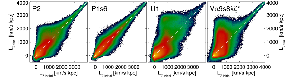
Figure 4: The distribution of thick-disc stars in the $L_{z}(t_{\rm initial})$-$L_{z}(t_{\rm f})$ plane. For thick-IC disc models we consider all IC stars at $t_{\rm initial}=0$, whereas for models with declining $\sigma_{0}$ we consider all stars born at $t\leq 2\,{\rm Gyr}$ and use $t_{\rm initial}=2\,{\rm Gyr}$. The white dashed line marks $L_{z}(t_{\rm initial})=L_{z}(t_{\rm f})$.

Model P1s6, which has hardly any migration, shows that the non-migrating IC stars are the hottest IC stars. Thus for our thick-disc ICs, the strength of migration determines whether outwards migrators heat the disc, but for realistic levels of radial migration they do heat it significantly.

The diagram looks quite different for Model V$\alpha$9s8$\lambda\zeta$*. The outwards migrators in the old, hot population of this model are cooler than the stars with $\Delta L_{z}=0$, in contrast to what was found in P2. For models of this class we assume a radially constant input dispersion $\sigma_{0}$ whereas the thick-disc ICs require an outwards declining vertical dispersion to maintain a constant scale height. Stars migrating outwards to lower surface densities and shallower potential wells will cool as they adiabatically conserve their vertical actions, whereas stars with $\Delta L_{z}=0$ will actually undergo mild adiabatic heating as the surface density increases with time.

In Model P2 the radial gradient in $\sigma_{z,{\rm thick}}$ caused outwards migrators to have a higher $\sigma_{z}$ at the start of the simulation than stars with $\Delta L_{z}=0$, and by $t=t_{\rm f}$ adiabatic cooling/heating of the populations has lowered but could not fully erase this initial difference. In Model V$\alpha$9s8$\lambda\zeta$* there was no initial radial gradient in $\sigma_{z,{\rm thick}}$ and thus outwards migrators have lower $\sigma_{z}$ than stars with $\Delta L_{z}=0$. The fact that, in P2, $\sigma_{z}$ drops at $\Delta L_{z}>1000\,{\rm kpc}\,{\rm km\,s^{-1}}$ indicates that the greater tendency of cooler stars to migrate modifies this picture. We do not know what the initial dispersion gradient in the MW looked like, as in this work we do not investigate the heating mechanism for the thick disc and thus we cannot draw conclusions regarding heating of the outer MW disc by migrators.

3.3 Migration of thick-disc stars

The chemically defined thick disc in the MW has recently been studied over an extended volume ($R=3-15\,{\rm kpc}$, $|z|=0-2\,{\rm kpc}$) by Hayden et al. (2015) using stars from the APOGEE survey. They show that very few stars of the high $\alpha$ sequence are found outside of $R\sim 11\,{\rm kpc}$. Inside this radius, the high-$\left[{\rm\alpha/Fe}\right]$ sequence inhabits the same area in the $\left[{\rm\alpha/Fe}\right]$-$\left[{\rm Fe/H}\right]$-plane. Chemical evolution models (Schönrich & Binney, 2009b) require that these stars must have formed at early times and at radii significantly inside $R_{0}$ and thus must have migrated outwards.

In our simulations, we do not model chemical evolution. Moreover, our galaxies by construction have for the IC disc and for the inserted stars exponential profiles, which do not have an outer cutoff for SF, as one would expect to find in real galaxies. Still, we can inspect the extent of radial migration by thick-disc stars and check (i) whether a significant number of stars from the inner galaxy have reached the Snhd, and (ii) whether at $t=t_{\rm f}$ there is a characteristic radius or angular momentum $L_{z}$, beyond which one is extremely unlikely to find an outwards migrator from the early disc.

In Figure 4 we therefore plot the distribution of thick-disc stars in the $L_{z}(t_{\rm initial})$-$L_{z}(t_{\rm f})$ plane. Thick-disc stars and $t_{\rm initial}$ are defined as follows: (i) for models with thick IC discs we consider all IC stars at $t_{\rm initial}=0$, and (ii) for models with declining $\sigma_{0}$ we consider all stars born at $t\leq 2\,{\rm Gyr}$ and use $t_{\rm initial}=2\,{\rm Gyr}$. The white dashed line marks $L_{z}(t_{\rm initial})=L_{z}(t_{\rm f})$. Considering a Snhd like region at $R=8\,{\rm kpc}$, the corresponding angular momentum for our models at $t=t_{\rm f}$ is in the range $L_{z}(t_{\rm f})=1800-2000\,{\rm kpc}\,{\rm km\,s^{-1}}$ for circular orbits. Note that stars on eccentric orbits spend more time near apocentre than near pericentre and thus the $L_{z}$ distribution at a given radius will be skewed towards lower $L_{z}$.

As discussed in previous sections, the migration in Model P1s6 is suppressed as the strength of non-axisymmetric structures is low at all times. Thus at $t=t_{\rm f}$ there are few thick-disc stars at values of $L_{z}$ typical for the Snhd. The situation is markedly different in the other three models shown. All of these models predict a significant number of outwards migrators in today’s Snhd from $L_{z}(t_{\rm initial})\la 500\,{\rm kpc}\,{\rm km\,s^{-1}}$. The distribution of stars with $L_{z}(t_{\rm f})=1800-2000\,{\rm kpc}\,{\rm km\,s^{-1}}$ is skewed towards lower $L_{z}(t_{\rm initial})$ and thus outwards migrators in these models. As already discussed in Section 3.2, the Snhd is more dominated by outwards migrators in Model V$\alpha$9s8$\lambda\zeta$* than in Model P2, because at early times V$\alpha$9s8$\lambda\zeta$* had both a more compact thick disc and stronger non-axisymmetries.

Models P2, U1 and V$\alpha$9s8$\lambda\zeta$* also show very little migration in the outer disc, as we find $L_{z}(t_{\rm initial})\approx L_{z}(t_{\rm f})$ for $L_{z}(t_{\rm initial})\ga 3000\,{\rm kpc}\,{\rm km\,s^{-1}}$. This is because in all models the outer discs are DM dominated and disc self-gravity is too weak to generate the non-axisymmetric structures required to drive significant radial migration.

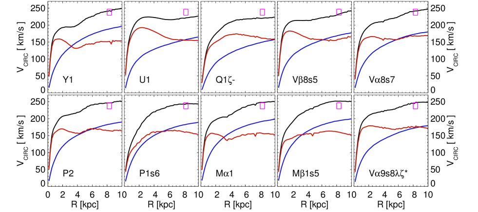
Figure 13: Circular speed curves $v_{\rm circ}(R)$ measured in the midplane of the disc. We determine the circular speed as $v_{\rm circ}=\sqrt{{a_{R}(R)}R}$, where $a_{R}(R)$ is the azimuthal average of the radial gravitational acceleration, $\partial\Phi/\partial R$. Blue lines mark the contributions from DM and red lines the baryonic contribution. Pink boxes mark the constraints on $R_{0}$ and $v_{\rm circ}(R_{0})$ determined by Schönrich (2012).

Moreover, these three models show that there is an effective upper boundary $L_{z,{\rm final,edge}}$ that the stars with low $L_{z}(t_{\rm initial})$ can reach. This boundary varies little with $L_{z}(t_{\rm initial})$ so long as $L_{z}(t_{\rm initial})<L_{z,{\rm final,edge}}$. The value of $L_{z,{\rm final,edge}}$ does vary from simulation to simulation: we find $L_{z,{\rm final,edge}}\approx 2300\,{\rm kpc}\,{\rm km\,s^{-1}}$ in P2, $L_{z,{\rm final,edge}}\approx 2800\,{\rm kpc}\,{\rm km\,s^{-1}}$ in V$\alpha$9s8$\lambda\zeta$* and $L_{z,{\rm final,edge}}\approx 3100\,{\rm kpc}\,{\rm km\,s^{-1}}$ in U1. The boundary reflects the absence of significant drivers of radial migration in the outer disc. $L_{z,{\rm final,edge}}$ is higher in U1 than P2, because U1 is baryon-dominated to a larger radius than P2 (Figure 13). This upper bound for $L_{z}(t_{\rm final})$ explains why Hayden et al. (2015) find that the chemically defined thick disc peters out at $R\sim 10\,{\rm kpc}$ and confirms that the outer-most stars of the chemically defined thick disc can be migrators from the early inner disc despite their being vertically hot.

4 Solar neighbourhood kinematics

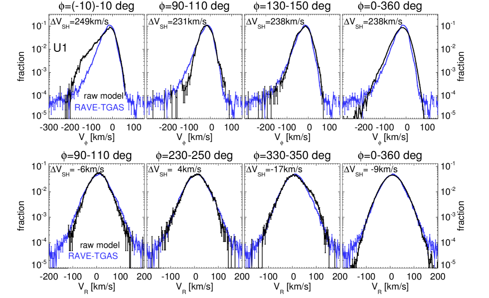
Figure 5: Azimuthal variation of in-plane velocity histograms in direction of rotation $V_{\phi}$ (top row) and radial direction $V_{R}$ (bottom row) in model U1 for three azimuthal bins each (left three columns) and an azimuthal average (right column). The numbers in the top left corners of each panel show the relevant component of $\Delta{\bf V}_{\rm sh}$ in $\,{\rm km\,s^{-1}}$, the velocity by which the model histograms were shifted. Here we consider only altitudes $|z|<250\,{\rm pc}$. Black points are model data and blue points are RAVE-TGAS data. Poisson error-bars are shown for all histograms.

4.1 RAVE-TGAS velocity distributions

Next we compare kinematics of model stars at different altitudes to data from the Gaia mission (Gaia Collaboration, 2016a). The release of Gaia data includes the Tycho-Gaia Astrometric Solution (TGAS, Gaia Collaboration, 2016b), which contains proper motions and parallaxes $\varpi$ for $\sim 2\times 10^{6}$ nearby stars. Combined with line-of-sight velocities $v_{\parallel}$ from the Radial Velocity Survey (RAVE, Kunder et al., 2017), 6D phase space information is available for $\sim 2.5\times 10^{5}$ stars.

4.1.1 RAVE-TGAS data

We use the catalogue provided by the 5th data release of the RAVE survey (Kunder et al., 2017), which contains $255\,922$ observations of stars to which TGAS counterparts have been assigned. As the catalogue contains multiple observations of certain stars, we first look for observations which have identical TGAS proper motions and parallaxes. For multiple observations of the same object we select the one with the smallest observational error in $v_{\parallel}$. We discard stars with negative parallaxes and stars with parallax errors $\sigma_{\varpi}>0.25\varpi$. For simplicity we assume that the distances $s$ of surviving stars can be calculated as the inverse of the parallaxes $\varpi$, $s=1/\varpi$. At the accuracy required for our comparison, this is a reasonable assumption as was shown by Schönrich & Aumer (2017). As the smallest parallax errors in TGAS are $\sigma_{\varpi,{\rm min}}\sim 0.21\;{\rm mas}$, distances are limited to $s\la 1.2\,{\rm kpc}$.

For the remaining $\sim 1.3\times 10^{5}$ stars we calculate positions in Galactic coordinates and the Cartesian components $U,V,W$ of heliocentric velocity, with $U$ directed towards the Galactic centre and $V$ in the direction of Galactic rotation. The components $U,V$ are then transformed into the component $V_{R}$ from the Galactic centre to the position of the star, and $V_{\phi}$ in the direction of a circular orbit at the position of the star. To determine $V_{R}$ and $V_{\phi}$, we require the in-plane velocities of the Sun in the Galactic rest frame and distance of the Sun to the Galactic centre, which Schönrich (2012) and Schönrich et al. (2010) determined as $V_{{\rm g},\odot}=250\,{\rm km\,s^{-1}}$, $U_{\odot}=11\,{\rm km\,s^{-1}}$ and $R_{0}=8.3\,{\rm kpc}$. We choose the zero points of $V_{R}$ and $V_{\phi}$ so that at the position of the Sun a star has $V_{R}=-U$ and $V_{\phi}=V$.

We bin the sample’s stars into the altitude ranges $|z|<250\,{\rm pc}$, $250\,{\rm pc}<|z|<500\,{\rm pc}$ and $500\,{\rm pc}<|z|<800\,{\rm pc}$ and create histograms of all three velocity components in all three ranges. For simplicity we assume Poisson errors $\sigma_{N}=\sqrt{N}$, where $N$ is the number of stars in a velocity bin of size $\Delta V=6\,{\rm km\,s^{-1}}$ for $V_{\phi}$ and $\Delta V=4\,{\rm km\,s^{-1}}$ for the other components.

4.1.2 Azimuthal variation of velocity distributions

To compare our models to the RAVE-TGAS data, we select stars at $R=8.3\pm 1.0\,{\rm kpc}$ and for them create histograms of $V_{z}$, $V_{R}$ and $V_{\phi}$ at the same three altitude ranges with the same bin sizes $\Delta V$. To understand the azimuthal variation of the velocity distribution, we divide the cylindrical shell into 18 equally sized parts, each 20 degrees wide and additionally create histograms for all azimuths combined. The angle between the line Sun-Galactic centre line and the major axis of the bar is usually assumed to be in the range $15-30$ degrees (see e.g. Binney et al., 1991; Wegg & Gerhard, 2013) on the trailing side of the bar. We define an angle $\phi$ for our models, such that the tips of the bar are at $\phi=0$ and $180$ degrees and the most likely Snhd bins are at $\phi=10-30$ and $190-210$ degrees.

To illustrate the azimuthal variations of the $V_{R}$ and $V_{\phi}$ distributions, we show in Figure 5 data from model U1, which, as was discussed in Paper 3, has a strong and unrealistically long bar. Consequently its distributions of $V_{R}$ and $V_{\phi}$ vary significantly with azimuth. By contrast its distribution of $V_{z}$ varies insignificantly, so we do not show them.

Given that the Sun has a velocity $U_{\odot}\simeq 11\,{\rm km\,s^{-1}}$ towards the Galactic Centre, the $R$ component of the measured heliocentric velocities of stars are larger than their Galactocentric velocities by $\Delta V_{R}\sim 11\,{\rm km\,s^{-1}}$. Hence in each panel of Figure 5 U1’s velocity histogram has been shifted by taking from the Galactocentric velocity a vector $\Delta{\bf V}_{\rm sh}$. For any given panel, we choose $\Delta{\bf V}_{\rm sh}$ to optimise the fit between the model histograms and the corresponding histograms of the velocities of RAVE-TGAS stars, which are plotted in blue. If the Galaxy were axisymmetric, the $R$ component of ${\bf V}_{\rm sh}$ would be the reflex of the Solar motion with respect to the Local Standard of Rest (LSR), so $\Delta V_{{\rm sh},R}=-6\,{\rm km\,s^{-1}}$ would imply $U_{\odot}=6\,{\rm km\,s^{-1}}$, and the $\phi$ component of $\Delta{\bf V}_{\rm sh}$ would be the sum $v_{\rm circ}+V_{\odot}$ of the local circular speed and the Sun’s peculiar azimuthal velocity. Since model U1 is strongly non-axisymmetric, the shifts required to optimise the fit to the RAVE-TGAS data vary with azimuth as shown at the top of each panel of Figure 5. These variations reflect the fact that the non-axisymmetric component of the potential causes the whole Solar neighbourhood to move in and out and to slow down and then speed up as it moves around the Galactic Centre.

The values of $\Delta{\bf V}_{\rm sh}$ given in Figure 5 were determined as follows. At a given azimuth $\phi$, we systematically shifted the model data in steps of $1\,{\rm km\,s^{-1}}$ independently in all three velocity components and used the same binning as applied for the Snhd data. Then for each component $V_{j}$ we computed the figure of merit

$$\chi^{2}=\sum_{i_{\rm min}}^{i_{\rm max}}{\bigl{(}n_{i,{\rm model}}-n_{i,{\rm data}}\bigr{)}^{2}\over\sigma_{n,i,{\rm model}}^{2}+\sigma_{n,i,{\rm data}}^{2}},$$ (9)

where $n_{i}\equiv N_{i}/N$ and $\sigma_{n,i}=\sqrt{N_{i}}/N$ with $N_{i}$ the number of stars in velocity bin $i$ and $N$ is the total number of stars at the given range in azimuths and altitudes. The sum runs between the minimum and maximum bins considered, the choice of which is not critical as long as the majority of stars are included because the bins in the wings of the distributions have low $N_{i}$ and thus contribute little to $\chi^{2}$. The values of $\Delta V_{\rm sh}$ given at the top of each panel of Figure 5 are those that minimise $\chi^{2}$.

The first row in Figure 5 shows $V_{\phi}$ distributions in model U1 at $|z|<250\,{\rm pc}$ for three different azimuthal bins and averaged over all $\phi$. At an angle $\phi$ aligned with the major bar axis in the range $(-10,10)$ degrees, the $V_{\phi}$ distribution of the model is much more skewed towards low $V_{\phi}$ than is that of the Snhd data, while in the range $(90,110)$ degrees, the model distribution drops more sharply at low $V_{\phi}$. In the range $(130,150)$ degrees, the model agrees reasonably with the Snhd data, but this azimuthal range is on the leading side of the bar. We note that the steep decline towards high $V_{\phi}$ is similar at all azimuths and agrees with the data, which is why our algorithm chooses $\Delta V_{{\rm sh},\phi}$ so the histograms agree roughly in this $V_{\phi}$ range. When all azimuthal bins are considered, $\Delta V_{{\rm sh},\phi}$ varies between $226$ and $249\,{\rm km\,s^{-1}}$. The top right panel shows that when we average over all azimuths, the model $V_{\phi}$ distribution is similar in shape but wider than the data distribution and we find an intermediate $\Delta V_{{\rm sh},\phi}=238\,{\rm km\,s^{-1}}$. The width of the distribution is determined by two factors: (i) the varying widths at different azimuths and (ii) the variation of $\Delta V_{{\rm sh},\phi}$, which broadens the distribution.

The second row in Figure 5 shows the $V_{R}$ distributions of model U1. The variation with $\phi$ is less pronounced than in the case of $V_{\phi}$. At $\phi=90-110$ degrees the distribution is narrowest, as for $V_{\phi}$. Close to the major bar axis (here $\phi=330-350$ degrees), we find a distribution which is skewed towards high $V_{R}$, whereas at $\phi=230-250$ degrees there is reasonable agreement with the Snhd data. Considering all azimuthal bins, $\Delta V_{{\rm sh},R}$ varies between $-23$ and $+4\,{\rm km\,s^{-1}}$. The azimuthally averaged histogram is again widened around $V_{R}\sim 0$ because of this systematic variation, but agrees reasonably well with the data.

We note that none of the model histograms show enough stars at the extreme wings of the Snhd velocity distributions. This is not worrying, as (a) observational velocity errors were not modelled and (b) halo stars are not included in the model. See Schönrich et al. (2011) for an illustration of how both points alter the $V_{\phi}$ distribution.

Figure 5 clearly shows that it is essential to choose an appropriate azimuth $\phi$ when comparing a model with non-axisymmetries to Snhd data. Both using an azimuthal average and choosing a wrong azimuth can lead to significantly misleading conclusions.

For most models, we find that $\Delta{\bf V}_{\rm sh}$ is not constant with altitude. At a Snhd-like value of $\phi$, $\Delta V_{{\rm sh},\phi}$ for most models decreases with increasing $|z|$ by up to $\sim 10\,{\rm km\,s^{-1}}$; only in a very few models does $\Delta V_{{\rm sh},\phi}$ increase with $|z|$. Most models show altitude variations of $\Delta V_{{\rm sh},R}$ smaller than $\pm 3\,{\rm km\,s^{-1}}$. These variations are not significant as the Poisson errors are large at higher latitudes. The strongest deviations are found in models with strong bars, such as U1, where we find $\Delta V_{{\rm sh},R}$ to be lower by $\sim 8\,{\rm km\,s^{-1}}$ at higher $|z|$. These variations with altitude are in part caused by differences in the shape of the velocity distribution between model and data. Uncertainties in the observations, which increase with distance and vary with Galactic latitude are also expected to play a role.

$\Delta V_{{\rm sh},z}$ usually shows very little variation with either azimuth or altitude. Typical values are in the range $\Delta V_{{\rm sh},z}=7-8\,{\rm km\,s^{-1}}$ in agreement with LSR determinations for the Snhd (e.g. Dehnen & Binney, 1998; Schönrich et al., 2010). In model U1 we find a mild systematic variation with altitude with lower shifts near the bar tips, $\Delta V_{{\rm sh},z}=6-7\,{\rm km\,s^{-1}}$, and higher shifts at $\phi\approx 90-130$ and $270-310$ degrees, $\Delta V_{{\rm sh},z}=8-9\,{\rm km\,s^{-1}}$.

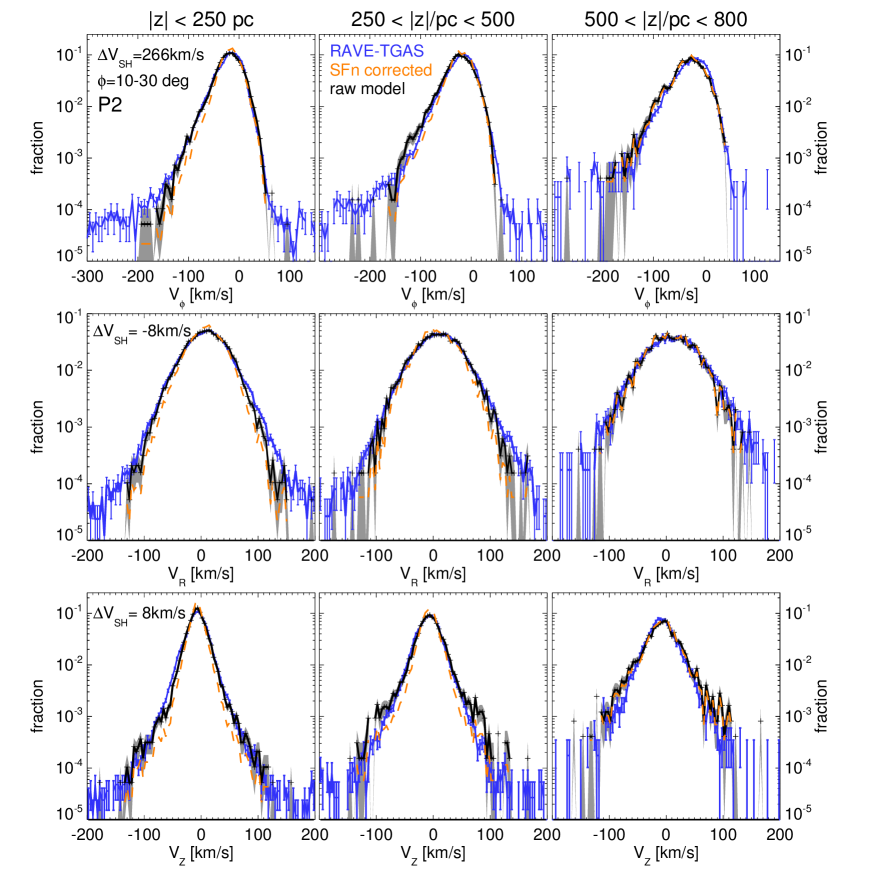
Figure 6: A comparison of velocity distributions in model P2 with RAVE-TGAS data. Each row shows a different component: $V_{\phi}$ top row, $V_{R}$ middle row and $V_{z}$ bottom row. Each column shows a different altitude bin: $|z|<250\,{\rm pc}$ (left), $250<|z|/\,{\rm pc}<500$ (middle) and $500<|z|/\,{\rm pc}<800$ (right). Snhd data with Poisson error-bars are shown in blue. Raw model histograms are shown in black with grey shaded areas marking the Poisson uncertainties. Model histograms altered by the selection function are shown as orange dashed lines. The number in the top left corner of each leftmost panel is the relevant component of the shift vector $\Delta{\bf V}_{\rm sh}$. The latter is determined for raw histograms. The azimuthal range considered is at an angle $\phi=10-30$ degrees to the major axis of the bar on the trailing side, similar to the Snhd. The radial range considered for the models is $R=8.3\pm 1.0\,{\rm kpc}$.

4.1.3 Selection function

When comparing our models to Snhd data we should consider the effects of survey selection functions (SFns), as was discussed in Paper 2 for the age SFn of the GCS data (see also Section 4.2). Here we only seek a qualitative understanding of the age SFn of our sample. To circumvent the spatial SFn (see Schönrich & Aumer, 2017), we consider stars at different altitudes $|z|$ as explained above. We do not expect significant variations of stellar kinematics over distances $s\la 1\,{\rm kpc}$ in the $R$ and $\phi$ directions.

For our spatially limited RAVE-TGAS sample as selected above, we consider the $I$-band magnitude selection of RAVE stars in the interval $9<I<12$ (Wojno et al., 2017) to dominate. To model the SFn, we employ the population synthesis machinery from the Schönrich & Binney (2009a) model as described in Section 2 of Aumer & Schönrich (2015). We find that for all distances $s\la 1\,{\rm kpc}$, the selection probability $p$ is well approximated by $p\propto{{1}/(\tau/\,{\rm Gyr}+1.5)}$, where $\tau$ is the age of the star.

To calculate SFn weighted velocity distributions, we replace the numbers of model particles in velocity bin $i$, $N_{i}$, with the effective number $N_{i,{\rm eff}}=\sum_{j}{w_{j}}$, where $w_{j}={{1}/(\tau_{j}/\,{\rm Gyr}+1.5)}$ is the SFn weight of star $j$. Poisson errors are calculated as

$$\sigma_{N_{i,{\rm eff}}}={{\sum_{j}{w_{j}}}\over{\sqrt{\sum_{j}{w_{j}^{2}}}}}.$$ (10)

The effect of this selection can be understood from Figure 6. The right column shows the velocity distributions of stars in model P2 at the highest altitude bin $500<|z|/\,{\rm pc}<800$, which is dominated by the thick-disc stars, which in this model come from the IC. Since the vast majority of those stars are old, there is little difference between the intrinsic distributions (black) and the SFn weighted distributions (orange). At lower altitudes, shown in the left and middle columns, the impact of the SFn is clearly visible. The SFn produces narrower velocity distributions for all velocity components because it prefers younger and thus kinematically cooler stars. The effect is somewhat stronger at intermediate altitudes, as they contain a more equal mixture of younger and older stars, whereas the lowest altitude bin has a high fraction of young stars. The distributions in $V_{\phi}$ are asymmetric and the SFn hardly affects the steep falloff towards higher velocities. As was e.g. shown in figure 2 of Schönrich & Binney (2012), hotter populations have their distributions strongly skewed towards lower $V_{\phi}$ and bins at high $V_{\phi}$ are thus always dominated by young and cool populations, so the SFn has little effect at high $V_{\phi}$.

4.1.4 Model P2

In Figure 6 we compare RAVE-TGAS data with the velocity distributions of Model P2 in one of the two possible Snhd locations: $R=8.3\pm 1.0\,{\rm kpc}$ and $\phi=10-30$ degrees. As the bar has $m=2$ symmetry, we can find locations near either end of the bar and choose the one that agrees best with the Snhd data. One has to keep in mind that we are not in any way fitting to the data. Model P2 existed before the TGAS data were published and was created with structural and AVR constraints in mind. The RAVE-TGAS data are thus an independent evaluation of our models. As was already noted, we do not model the effect of halo stars and observational errors and thus do not expect agreement between model and data in the extreme wings of the distributions. For model P2, the discrepancies appear roughly at $|V_{R}|>100\,{\rm km\,s^{-1}}$, $|V_{z}|>120\,{\rm km\,s^{-1}}$, $V_{\phi}>50\,{\rm km\,s^{-1}}$ and $V_{\phi}<-150\,{\rm km\,s^{-1}}$.

The data for model P2 agree best with the observations when the SFn is not taken into account (black points and grey shaded error regions). Indeed then for all velocity components the model agrees quite well with the observations at all altitudes. Applying the SFn (orange dashed line) generally makes the model velocity distributions too narrow except in the highest altitude bin, where the SFn has no significant impact.

Considering the raw $V_{\phi}$ distributions in the relevant regions, we find good agreement at all scaleheights. At $500<|z|/\,{\rm pc}<800$, the centre of the distribution is shifted to lower $V_{\phi}$ than in the data. As already noted, if our algorithm is allowed to choose separate $\Delta{\bf V}_{\rm sh}$ at different altitudes, for most models it chooses lower $\Delta V_{{\rm sh},\phi}$ at higher $|z|$, in this case $5\,{\rm km\,s^{-1}}$ lower. At $250<|z|/\,{\rm pc}<500$, a $3\,{\rm km\,s^{-1}}$ difference in $\Delta V_{{\rm sh},\phi}$ would allow for an even better fit. At low $|z|$, and for all three altitude bins combined, we find $\Delta V_{{\rm sh},\phi}=266\,{\rm km\,s^{-1}}$. We should compare this to the Galactic rest frame velocity component in rotational direction $V_{{\rm g},\odot}=250\pm 9\,{\rm km\,s^{-1}}$ as found by Schönrich (2012). This paper suggests that $V_{{\rm g},\odot}$ comprises a local circular speed $v_{{\rm circ}}=238\pm 9\,{\rm km\,s^{-1}}$ and a motion relative to the LSR $V_{\odot}=12\pm 2\,{\rm km\,s^{-1}}$. From Figure 13, we learn that the azimuthally averaged $v_{{\rm circ}}\approx 247\,{\rm km\,s^{-1}}$ is at the upper end of the range allowed for the Snhd, which leaves a discrepancy of $\sim 7\,{\rm km\,s^{-1}}$ for $V_{\odot}$. As already noted, $\Delta V_{{\rm sh},\phi}$ varies with azimuth $\phi$, for this model at $|z|<250\,{\rm pc}$ between $252$ and $268\,{\rm km\,s^{-1}}$ as shown by the blue line in the lower panel of Figure 7. The other possible Snhd location ($\phi=190-210$ degrees) has $\Delta V_{{\rm sh},\phi}=261\,{\rm km\,s^{-1}}$ and a narrower $V_{\phi}$ distribution.

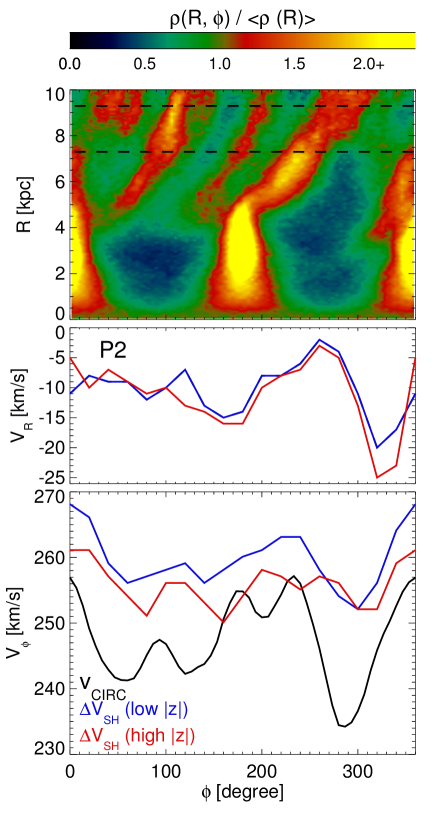
Figure 7: Bottom panel: the azimuthal variation at $R=8.3\,{\rm kpc}$ in model P2 of the circular speed $v_{\rm circ}=\sqrt{{a_{R}(R)}R}$ (black), the $\phi$ component of the velocity shift $\Delta{\bf V}_{\rm sh}$ found for altitudes $0<|z|/\,{\rm pc}<250$ (blue) and for $500<|z|/\,{\rm pc}<800$ (red). Middle panel: azimuthal variation of the $R$ component of the velocity shift. Top panel: non-axisymmetries in P2 in the $R$-$\phi$-plane as traced by the overdensity $\rho(\phi,R)/\langle\rho(R)\rangle$. Dashed lines mark the region $R=8.3\pm 1.0\,{\rm kpc}$, used for velocity distributions.

Figure 7 shows that, along the direction of one bar tip, $\Delta V_{{\rm sh},\phi}$ has a maximum and the minima lie close to minor axis. Another maximum lies not along the other bar tip, as one would expect if the bar was completely dominant, but at $\phi\approx 240$ degrees. To understand this better, the black curve in the lower panel of Figure 7 shows the azimuthal variation of $v_{\rm circ}\equiv\sqrt{{a_{R}(R)}R}$. We calculate $v_{\rm circ}$ at three radii $R=7.8$, $8.3$ and $8.8\,{\rm kpc}$ and $54$ equally spaced azimuths $\phi$ each. Then we average over 3x3 points each to reduce $N$-body noise and determine $v_{\rm circ}(\phi,R=8.3\,{\rm kpc})$, which we find varies between $234$ and $256\,{\rm km\,s^{-1}}$ and thus by slightly more than $\Delta V_{{\rm sh},\phi}$. The curves are offset by $\sim 10-15\,{\rm km\,s^{-1}}$ because $V_{\odot}=12\pm 2\,{\rm km\,s^{-1}}$, but the positions of the extrema agree well. The variations are smaller in $\Delta V_{{\rm sh},\phi}$ than $v_{\rm circ}$ because the stars have a non-negligible velocity dispersion. The red line shows $\Delta V_{{\rm sh},\phi}$ for $500<|z|/\,{\rm pc}<800$, a region dominated by kinematically hotter thick-disc stars. Consequently, the variations are smaller than at $|z|<250\,{\rm pc}$, where thin-disc stars dominate. As noted above, at higher $|z|$ the model stars lag the thin-disc stars more than in the Snhd, so the red curve lies at lower $V_{\phi}$ than the blue curve.

To understand the deviation from a simple $m=2$, bar-dominated picture, we show in the upper panel of Figure 7 the azimuthal stellar density variation due to non-axisymmetries, tracked by the fractional azimuthal variation $\rho(\phi,R)/\langle\rho(R)\rangle$ in the $R$-$\phi$ plane. Clearly, at $R<5\,{\rm kpc}$, the bar dominates, as we can also learn from Figure 15. Outside $R=5\,{\rm kpc}$ and in the region $R=8.3\pm 1.0\,{\rm kpc}$, from which we select stars for our velocity histograms, a four-armed spiral pattern is visible, which itself shows significant substructure. The density peaks and troughs clearly correlate with the structure in the $v_{\rm circ}(\phi)$ curve – for example the bar-related minimum at $\phi\approx 280$ degrees is enhanced by a spiral arm which at these azimuths lies beyond $R=8\,{\rm kpc}$. We have no reason to believe that the model’s spiral structure provides a close match to the Galaxy’s spiral structure – we have shown that P2’s bar has a reasonable length but have not shown that its spiral structure resembles that of the Galaxy. Hence we should not expect the model curves to reproduce the observations in more than general characteristics.

Figure 7 suggests that non-axisymmetric structures cause the considered region in model P2 to move at $\Delta V_{\phi}\sim 7\,{\rm km\,s^{-1}}$ relative to the average circular velocity. We note that Bovy et al. (2012c) find $v_{{\rm circ}}=218\pm 6\,{\rm km\,s^{-1}}$ and $V_{{\rm g},\odot}=242^{+10}_{-3}\,{\rm km\,s^{-1}}$ for the Snhd and attribute the large difference $\sim 25\,{\rm km\,s^{-1}}$ to the sum of $V_{\odot}\sim 12\,{\rm km\,s^{-1}}$ and a systematic motion of the Snhd relative to the average circular velocity at $R_{0}$ of order $\Delta V_{\phi}\sim 10-15\,{\rm km\,s^{-1}}$. This proposed difference is even larger than that found in model P2.

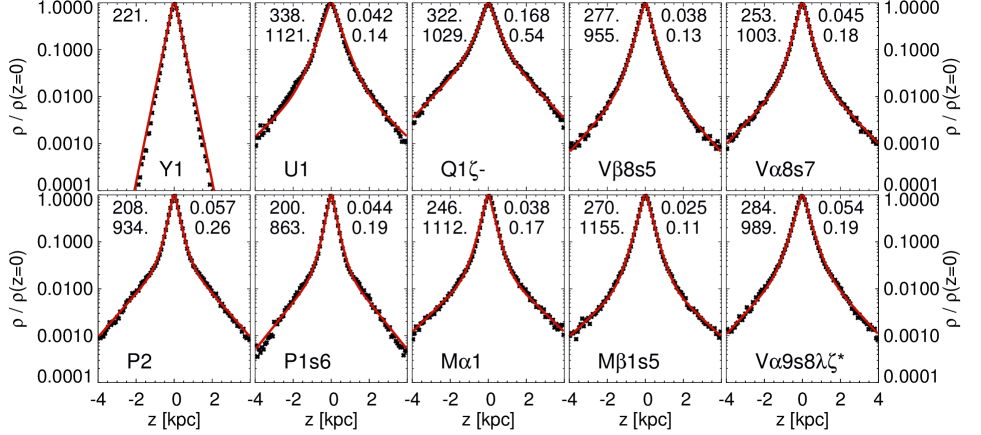
Figure 12: Vertical profiles of models at $t=t_{\rm f}$ and $R=8\pm 0.5\,{\rm kpc}$ are shown as black points. Overplotted are fits of $\rho(z)=\rho_{0}[\exp(-|z|/h_{\rm thin})+f\exp(-|z|/h_{\rm thick})]$ to these profiles. The numbers in the upper left corners are the values of the thin and thick disc scaleheights $h_{\rm thin}$ and $h_{\rm thick}$ in pc. The numbers in the upper right corners are the values of the density ratio $f$ and the surface density ratio $f_{\Sigma}=fh_{\rm thick}/h_{\rm thin}$. Y1 has no thick disc.

In the altitude bin $|z|<250\,{\rm pc}$, which is dominated by the thin disc, the radial and vertical velocity distributions are both somewhat too narrow, even when the SFn is neglected. This is interesting because P2’s thin-disc scaleheight, $h_{z,{\rm thin}}\approx 210\,{\rm pc}$, suggests an unrealistically narrow $V_{z}$ distribution (see Figure 12), but Paper 1 suggests that the appropriate level of migration and bar length should correspond to an appropriate radial velocity dispersion.

At higher $|z|$, the distributions of $V_{z}$ when the SFn is neglected are slightly too broad, whereas the corresponding $V_{R}$ distributions are slightly too narrow. P2 at higher altitude is dominated by the thick IC stars, which were set up with $\sigma_{R}/\sigma_{z}=1$. The comparison with the Snhd data suggests that $\sigma_{R}>\sigma_{z}$ might be more appropriate.

An offset $\Delta V_{{\rm sh},z}=8\,{\rm km\,s^{-1}}$ is in agreement with the solar peculiar velocity $W_{\odot}=7.3\pm 1\,{\rm km\,s^{-1}}$ found by Schönrich et al. (2010). We similarly find $\Delta V_{{\rm sh},R}=-8\,{\rm km\,s^{-1}}$. Bearing in mind that $V_{R}=-U$, this is only slightly inconsistent with the solar peculiar motion $U_{\odot}=11\pm 1\,{\rm km\,s^{-1}}$ found by Schönrich et al. (2010). For the RAVE-TGAS sample of Schönrich & Aumer (2017), $U_{\odot}\sim 10\,{\rm km\,s^{-1}}$ is favoured. We note that we are not expecting to be able to determine $U_{\odot}$ precisely with our method, as the detailed shapes of the $V_{R}$ velocity distributions differ between model and data. Additionally, there is a likely connection between $-\Delta V_{{\rm sh},R}$ being lower than $U_{\odot}$ and the streaming motions of this region in the model relative to a hypothetical circular orbit, as discussed above for $V_{\phi}$ and $V_{\odot}$. Indeed, the middle panel of Figure 7 shows that at both low and high $|z|$, $\Delta V_{{\rm sh},R}$ varies with $\phi$ between $-20$ and $-2\,{\rm km\,s^{-1}}$.

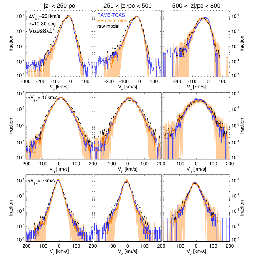
Figure 8: Same as Figure 6 but for model V$\alpha$9s8$\lambda\zeta$*. Distributions considering SFns are shown as orange points with shaded areas showing the Poisson uncertainties. Dashed black lines are for not taking the SFn into account. The shift vector $\Delta{\bf V}_{\rm sh}$ was determined using histograms which take into account the SFn. The components of $\Delta{\bf V}_{\rm sh}$ are shown in the top left corners of the first row panels.

4.1.5 Model V$\alpha$9s8$\lambda\zeta$*

In Figure 8, we compare velocity distributions from Model V$\alpha$9s8$\lambda\zeta$* with the RAVE-TGAS data. We chose V$\alpha$9s8$\lambda\zeta$* as a counterpart to P2 because it is a model for which the intrinsic velocity distributions (black dashed lines) are generally too wide at low and intermediate $|z|$, whereas the SFn adjusted distributions (orange points with shaded areas for Poisson errors) show good agreement overall. This difference arises because: (i) the thin disc in V$\alpha$9s8$\lambda\zeta$* is thicker than that in P2, (ii) its vertical velocity dispersions are generally higher than those in P2 (Figure 3) and (iii) its thick disc is radially hotter because disc stars were inserted with $\lambda=\sigma_{R}/\sigma_{z}=1.25$, whereas P2’s IC thick disc was set up with $\lambda=1$.

As in the case of P2, out of the two possibilities, we have chosen the Snhd-like location which shows the better agreement with data. We note that the stars of the low-mass elliptical IC used for V$\alpha$9s8$\lambda\zeta$* are included in the histograms. At $R=8.3\pm 1.0\,{\rm kpc}$ these form a very low density, halo-like component and add to the wings of the velocity distributions, but they are not an appropriate halo model for the Snhd as can be seen at low $V_{\phi}$.

If we consider the SFn adjusted $V_{\phi}$ distributions of V$\alpha$9s8$\lambda\zeta$*, we find a mild overproduction of stars with $V_{\phi}\approx 60\,{\rm km\,s^{-1}}$ at low $|z|$, good agreement at intermediate $|z|$ and mild tension at high $|z|$. This tension results both from a somewhat broader $V_{\phi}$ distribution in the model and a lower $V_{\phi}$ for the peak of the distribution. The latter is reflected in the fact, that, for $500<|z|/\,{\rm pc}<800$ only, we find a value of $\Delta V_{{\rm sh},\phi}$ that is lower by $9\,{\rm km\,s^{-1}}$, suggesting that the thick disc in the model lags the thin disc more than is the case in the Snhd.

At the chosen location we find $\Delta V_{{\rm sh},\phi}=261\,{\rm km\,s^{-1}}$. At the other possible Snhd location we find $\Delta V_{{\rm sh},\phi}=260\,{\rm km\,s^{-1}}$ and a slightly broader $V_{\phi}$ distribution. $\Delta V_{{\rm sh},\phi}$ varies between $253$ and $262\,{\rm km\,s^{-1}}$ for all azimuthal bins, a smaller amplitude of variation than in P2. The azimuthal variation in $v_{\rm circ}$ is between $243$ and $252\,{\rm km\,s^{-1}}$, so that our conclusions regarding the azimuthal variation of $V_{\phi}$ average velocities and the LSR are the same as for P2.

Taking into account the SFn, The $V_{R}$ distributions of model V$\alpha$9s8$\lambda\zeta$* agree very well with the RAVE-TGAS data at all values of $|z|$ considered here. The $V_{z}$ distributions of V$\alpha$9s8$\lambda\zeta$* are slightly narrower at lower and intermediate $|z|$. For the highest $|z|$ bin, we find good agreement for both $V_{z}$ and $V_{R}$. These altitudes are dominated by thick-disc stars, which in this model were fed to the model galaxy with hot birth dispersions and the assumption $\lambda=\sigma_{R}/\sigma_{z}=1.25$. This choice of the ratio appears to be more appropriate than $\lambda=1$, which was used for the thick-disc IC of model P2. Combining the information from models P2 and V$\alpha$9s8$\lambda\zeta$* and the RAVE-TGAS data, we can still confirm that $\lambda$ for the thick disc is significantly lower than the $\lambda\approx 1.7-2.5$ typically found for the thin disc (see Paper 2), as was discussed by Piffl et al. (2014), who argued for $\lambda\approx 1$ in the MW thick disc.

$\Delta V_{{\rm sh},z}$ is stable at $7\,{\rm km\,s^{-1}}$ for model V$\alpha$9s8$\lambda\zeta$*, and for $V_{R}$ we find $\Delta V_{{\rm sh},R}=-10\,{\rm km\,s^{-1}}$ in the Snhd like location shown in Figure 8. Both numbers are in in agreement with the vertical LSR velocities $W_{\odot}=7\pm 1\,{\rm km\,s^{-1}}$ and $U_{\odot}=11\pm 1\,{\rm km\,s^{-1}}$ found by Schönrich et al. (2010).The variation of $\Delta V_{{\rm sh},R}$ with $\phi$ in V$\alpha$9s8$\lambda\zeta$* is between $-17$ and $-4\,{\rm km\,s^{-1}}$, again a smaller variation compared to P2 and generally underlying the conclusions drawn from model P2.

4.2 Age Velocity Dispersion Relations

We have now established that the overall velocity distributions in our models with realistic bars and appropriate levels of migration closely reproduce Snhd velocity distributions. However, it is hard to quantify which models are best on account of uncertain selection effects.

The AVRs extracted from the GCS by Nordström et al. (2004) provide an additional constraint on Snhd kinematics. The GCS is restricted to stars at small distances $s\la 100\,{\rm pc}$, a volume that is under-represented in RAVE-TGAS. Paper 1 showed that the observed radial and vertical AVRs are reproduced by models that lack a thick disc but have a thin disc and a dark halo with appropriate masses and the right quantity of GMCs. Paper 2 showed further that the SFn of the GCS can hide an old thick-disc population because the GCS contains predominantly young stars and its age errors are significant. Whereas the models discussed in Papers 1 and 2 did not have thick discs, the models discussed here do.

4.2.1 Extracting AVRs from data and models

The green ($\sigma_{z}$) and red ($\sigma_{R}$) points in Figure 9 are the AVRs yielded by the ages and velocities of GCS stars given in Casagrande et al. (2011). As detailed in Paper 2, these AVRs are obtained by first excluding stars with halo characteristics and then selecting stars with ‘good’ age determinations. The remaining $\sim 7\,500$ stars are sorted by age and the velocity dispersions $\sigma_{i}(\tau)$ of groups of 200 adjacent stars are computed, with a new group being formed after moving ten stars down the rank. Hence every 20th value of $\sigma_{i}(\tau)$ is statistically independent of its predecessors.

To determine the AVRs of a model, we select stars satisfying $R=8.3\pm 0.5\,{\rm kpc}$ and $|z|<100\,{\rm pc}$. As detailed in Paper 2, these stars are then sorted in age $\tau$ and assigned weights $w(\tau)$, so that their weighted age distribution agrees with that of the GCS sample. For models with thick-disc ICs, which all have $t_{\rm f}=10\,{\rm Gyr}$, stars in the ICs are assigned ages $\tau_{\rm IC}\in(10,12)\,{\rm Gyr}$. A model in which $\sigma_{0}$ declines is considered only if $t_{\rm f}=12\,{\rm Gyr}$, and in such a model we exclude stars from the low-density elliptical ICs as being ‘halo’ stars. Finally, we simulate the impact of age errors by scattering the age of each star through a Gaussian distribution with dispersion $\sigma_{\tau}=0.2\tau$.

The black lines in Figure 9 are for all stars in the selected volume. The grey lines are for subsets made by dividing the volume in 18 azimuthal bins of equal width. The blue lines are for the bins at $\phi=10-30$ and $190-210$ degrees and thus at locations relative to the bar similar to that of the Snhd. The pink lines show the intrinsic AVRs, before correction for age bias and errors, and averaged over all azimuths.

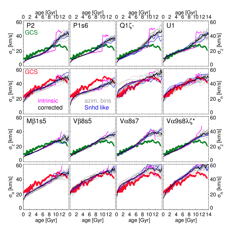
Figure 9: Radial and vertical AVRs in various models. The first and third rows show $\sigma_{z}(\tau)$ and the second and fourth rows show $\sigma_{R}(\tau)$. Green and red points are data extracted from Casagrande et al. (2011) as described in the text. Black curves are model AVRs at $R=8.3\pm 0.5\,{\rm kpc}$, $|z|<100\,{\rm pc}$ and $t=t_{\rm f}$ adjusted for age bias and errors. Grey curves are the same for 18 equally spaced azimuthal bins of the same spatial region. Blue lines are for azimuthal bins which lie in Snhd-like positions relative to the bar. The pink lines show the intrinsic AVRs without correction for age bias and errors for all azimuths.

4.2.2 AVRs in thin+thick disc models

We start by discussing the P models, which live in dark haloes with concentration parameter $c=9$. Paper 1 showed that in such haloes thin-disc models (Y models) with a mass of $M_{\rm f}=5\times 10^{10}\,M_{\odot}$ reproduce the GCS data quite well. The pink curves in Figure 9 show that at $\tau=10\,{\rm Gyr}$, the thick-IC disc of a P model generates steps in the pink curves for both the intrinsic $\sigma_{z}$ and the intrinsic $\sigma_{R}$, with the step in $\sigma_{z}$ being more pronounced. After correction for age bias and observational errors, the radial AVR of Model P2 (black curve) is still a reasonable match to Snhd AVR, but only on account of the presence of thick-IC stars. The corrected vertical AVR does not fit the data well: in the model $\sigma_{z}$ is too large at $\tau>10\,{\rm Gyr}$ and too small at $\tau<7\,{\rm Gyr}$. The vertical AVR of Model P1s6 is similar to that of Model P2, but the radial AVR is too low at all ages.

So both these P models point to inefficient radial heating, especially at early times. In Model P1s6, the shortfall in $\sigma_{R}$ is caused by a lack of non-axisymmetric structure that was already discussed in Section 3. Model P2, which at $t=t_{\rm f}$ has a more compact stellar disc than P1s6, shows a bar and a four-arm spiral pattern (see Figure 7) and sufficient radial migration over the last $5\,{\rm Gyr}$. The non-axisymmetries, however, emerge relatively late (see Figure 14), explaining the low values of $\sigma_{R}$ for old thin-disc stars. As regards vertical AVRs, the low dispersions of young stars are associated with relatively low thin scaleheights $h_{z,\rm thin}\approx 205\,{\rm pc}$ in both P2 and P1s6 (see Figure 12). In fact, the intrinsic vertical dispersions of the thin-disc stars are cooler than those in corresponding thin-disc only models at all ages.

Several factors contribute to the unrealistically low values of $\sigma_{z}$ in P models:

• The Y models presented in Paper 2 do not all reproduce the Snhd AVRs well – Y2, the model corresponding to P2, does show slightly lower $\sigma_{z}(\tau)$ at almost all $\tau$ as shown in Figure 2 of Paper 2. The IC disc masses of P models are three times higher than those of Y models, and at a given final mass $M_{\rm f}$ the SFRs are thus lower. Consequently, for a given value of $\zeta$, a P model has fewer GMCs, and thus less vertical heating.

• Paper 2 showed that the efficiency of GMC heating depends on the mass fraction of GMCs. Due to the additional mass in the ICs, the GMC mass fraction is lower in P models and heating is reduced.

• In Figure 3, we showed that when the vertical dispersions are determined by GMC heating, stars that have migrated outwards show higher dispersions than non-migrated stars. As migration levels in P1s6 are suppressed and in P2 are only high at late times, $\sigma_{z}$ is lower than in corresponding Y models, especially for old stars.

• Paper 1 showed that clustering of GMCs in spiral structures has a mild, but strengthening effect for vertical disc heating. As structure is suppressed in P models, this also weakens vertical heating.

Consider now Model M$\beta$1s5, which has declining $\sigma_{0}$, $M_{\rm f}=5\times 10^{10}\,M_{\odot}$ and lives in a dark halo with a high concentration parameter $c=9$. In this model $\sigma_{R}$ and $\sigma_{z}$ are both low at young ages notwithstanding the model’s larger thin-disc scaleheight, $h_{z,\rm thin}\approx 270\,{\rm pc}$. Its non-axisymmetric structure is too weak, so it shows too little radial migration. These characteristics arise from too little disc self gravity. Since the circular speed curves of Figure 13 of models with $c=9$ already have $v_{\rm circ}(R_{0})$ at or above the upper allowed limit, the lack of disc self-gravity can only be remedied by reducing the halo density, for example by decreasing $c$. Thus, models with a massive thick disc require a smaller value of $c$ than a similar model with just a thin disc. An enhanced baryon contribution to the gravitational field in the inner galaxy is also required for satisfaction of the microlensing constraints, as discussed in Section 4.4 of Paper 3.

Paper 1 showed that lowering $c$ makes discs more unstable and by $c=4$ the disc is too radially hot. From Figure 7 of Paper 3, we know that $c=6-7.5$ gives models which agree with the locally measured DM density. As representatives of models with $c<9$ and a thick-IC disc, we here discuss (i) Q1$\zeta$-, which has $c=6.5$, a more massive IC disc, $M_{\rm disc,i}=2.5\times 10^{10}\,M_{\odot}$, than a P model, and thus a higher final galaxy mass $M_{\rm f}=6.0\times 10^{10}\,M_{\odot}$, and (ii) U1 which has $c=7.5$, $M_{\rm disc,i}=2.0\times 10^{10}\,M_{\odot}$ and $M_{\rm f}=6.0\times 10^{10}\,M_{\odot}$.

Lowering $c$ and increasing $M_{\rm f}$ produces stronger non-axisymmetric structures. For model Q1 (not shown, see Paper 3), this results in an unrealistically long bar – it extends to $R\sim 8\,{\rm kpc}$. Lowering $\zeta$ for model Q1$\zeta$- and thus increasing the number of GMCs yields a hotter thin disc and a weak, short $R\sim 4\,{\rm kpc}$ bar with a strong two arm spiral pattern at outer radii. The azimuthally averaged and error-corrected radial AVR (black line) is slightly too hot at most ages on account of the strong spiral pattern, but the vertical AVR is reasonable for young ages on account of the additional GMCs compared to the P models studied above. As in the P models, at old ages the vertical dispersions are excessive. Interestingly, choosing a Snhd-like location relative to the bar (blue lines) yields lower dispersions for both radial and vertical directions. We note that the azimuthal variation is dominated by the spiral pattern and the location of the Snhd relative to the bar is likely not relevant here.

The bar of Model U1 extends to $R\sim 6\,{\rm kpc}$ with a very extended X structure (Figure 12 of Paper 3). Apart from the unrealistically hot vertical dispersions at old ages caused by the thick disc, its azimuthally averaged AVRs agree well with Snhd data. The higher vertical dispersions than in other models with $\zeta=0.08$ are caused by the long bar, as was discussed for the similarly long and X-shaped bar of Model E2 of Paper 2. The blue lines representing Snhd-like locations tend to show slightly higher dispersions compared to the average. So models with thick-disc ICs with $c\sim 7$ indeed provide better agreement with Snhd data, but their morphologies are not appropriate.

The V models shown in Figure 9 live in a $c=6.5$ dark halo and start from low-mass elliptical ICs, which, however, have negligible impact on their evolution. They all have final masses $M_{\rm f}=6\times 10^{10}\,M_{\odot}$. These models fit the Snhd vertical AVR for stars with ages $\tau<7\,{\rm Gyr}$ (which are not affected by the thick-disc excess) better than any P model or the standard Y models of Paper 2. In these models the shape of thick-disc excess in both the intrinsic and the corrected AVRs differs from the corresponding excesses in models with thick ICs because the thick disc has an intrinsic AVR only in models with declining $\sigma_{0}$. Also in these models, input dispersions $\sigma_{0}$ are at all times higher than the $6\,{\rm km\,s^{-1}}$ used in all the four thick-IC disc models shown in Figure 9 (see curves in Figure 1). At early times, high $\sigma_{0}$ is responsible for the thick-disc formation, whereas GMC heating determines the final $\sigma_{z}$ for thin-disc stars (see Section 4.2.3).

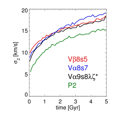
Figure 10: Heating histories $\sigma_{z}(t)$ for stellar populations which at $t=t_{\rm f}$ live at $R=8\,{\rm kpc}$ and are $\tau=5\,{\rm Gyr}$ old as traced from their birth to $t=t_{\rm f}$.

Model V$\beta$8s5 provides a very good match to the radial AVR of the Snhd. It grows inside out from $h_{R}=1.5$ to $4.3\,{\rm kpc}$ as $h_{R}\propto t^{0.5}$ and has an $\rm{SFR}\propto\exp(-t/8\,{\rm Gyr})$. At $t=t_{\rm f}$ it has a bar to $R\sim 4\,{\rm kpc}$ and it shows an appropriate level of radial migration over the last $5\,{\rm Gyr}$. Model V$\alpha$8s7 has the same radial growth history $h_{R}(t)$, but a different shape of $\sigma_{0}(t)$ and an ${\rm SFR}\propto\exp(-t/12\,{\rm Gyr}-0.5\,{\rm Gyr}/t)$, so the ${\rm SFR}$ grows initially before peaking at $t=2.5\,{\rm Gyr}$ and then declining. Consequently, $\sigma_{0}$ has to stay high longer to allow for enough thick-disc stars to form. This explains why the thick-disc excess in $\sigma_{z}(\tau)$ is shifted to lower ages. This ${\rm SFR}$ also provides more GMCs and a higher GMC mass fraction at late times, which is why it has slightly higher $\sigma_{z}(\tau)$ at low ages than V$\beta$8s5. In it $\sigma_{R}$ is slightly too large at most ages, which is likely connected to its unrealistically large surface density $\Sigma_{b}(R=8\,{\rm kpc})$, similar to that of V$\alpha$9s8$\lambda\zeta$* shown in Figure 8 of Paper 3, as it otherwise has a bar of reasonable length, $R\la 4\,{\rm kpc}$, and a reasonable level of radial migration.

Model V$\alpha$9s8$\lambda\zeta$* grows inside out from $h_{R}=1.0$ to $3.5\,{\rm kpc}$ as $h_{R}\propto t^{0.6}$ and has $\rm{SFR}\propto\exp(-t/6\,{\rm Gyr})$. Both these characteristics make it more compact than the other V models, especially at early times. To bring the GMC numbers at late times, and thus vertical heating, to similar levels, it has a lower value of $\zeta=0.06$. It also has an unrealistically high surface density $\Sigma_{b}(R=8\,{\rm kpc})$ and values of $\sigma_{R}$ that are slightly too high at intermediate ages. For the oldest ages, it shows the highest radial dispersions. This comes from the fact that it has $\lambda=1.25$, i.e. $\sigma_{R}=1.25\sigma_{0}$ and thus higher radial input dispersions at early times. Consequently, the oldest stars in V$\alpha$9s8$\lambda\zeta$* have unrealistically high values of both $\sigma_{z}$ and $\sigma_{R}$.

4.2.3 Thin-disc heating in models with declining $\sigma_{0}$

Whereas in models with declining $\sigma_{0}$ the final velocity dispersions of old stars are mainly determined by the value of $\sigma_{0}$ at early times, the value of $\sigma_{z}(\tau)$ measured for the thin disc at $t=t_{\rm f}$ and $R=8\,{\rm kpc}$ is insensitive to $\sigma_{0}$. Figure 10 shows that thin-disc stars are significantly heated by GMCs. To make this plot we constructed for several models heating histories of the stars with ages $\tau=5\pm 0.05\,{\rm Gyr}$ that at $t_{\rm f}$ are at $R=8\pm 0.5\,{\rm kpc}$. As detailed in Paper 2, we tracked these stars back in time through the simulation snapshots until their birth, and at each time determined the velocity dispersion of the population.

According to Figure 1, in the three V models shown in Figure 10 the input dispersion is $\sigma_{0}=10-15\,{\rm km\,s^{-1}}$, but when $\sigma_{z}$ is measured for a recently born population we obtain a lower value than $\sigma_{0}$ as all stars are born at $z=0$ and they will lose vertical kinetic energy as they all move away from the plane. Consequently, Figure 10 shows the vertical birth dispersion of these populations to be $\sigma_{z}(t_{\rm birth})=8-10\,{\rm km\,s^{-1}}$ and thus only slightly higher than that of young stars in the Snhd today. As a comparison, the green curve shows $\sigma_{z}(\tau)$ in Model P2, in which $\sigma_{0}=6\,{\rm km\,s^{-1}}$. Already Paper 2 showed that slightly increasing $\sigma_{0}$ improves the fit to the vertical AVR of the Snhd.

The velocity dispersions in all models shown in Figure 10 increase significantly over the $5\,{\rm Gyr}$ from birth to $t=t_{\rm f}$, and in all models the shape of $\sigma_{z}(t)$ is similar. The fact that $\sigma_{z}(t_{\rm birth})$ is lower in V$\alpha$8s7 than in V$\beta$8s5, but $\sigma_{z}(t_{\rm f})$ is higher shows that the details of GMC heating differ from model to model, as expected.

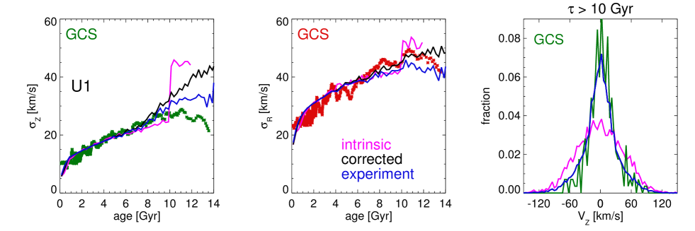
Figure 11: Assigning cool stars to old ages. Left panel: green points are the GCS vertical AVR $\sigma_{z}(\tau)$; the pink curve is the intrinsic AVR of model U1; the black line is the corrected AVR for all azimuths as in Figure 9 and the blue line is the experiment with randomly assigning ages to 3 per cent of stars from the weighted age distribution. Middle panel: the same for radial AVRs $\sigma_{R}(\tau)$ with GCS data in red. Right: $V_{z}$ histograms for stars with $\tau>10\,{\rm Gyr}$ in our GCS sample (green), for true ages from U1 (pink) and for the experiment (blue).

4.2.4 The connection between AVRs and RAVE-TGAS data

We have seen that Model P2 provides the better representation of the Snhd AVR for $\sigma_{R}$, whereas Model V$\alpha$9s8$\lambda\zeta$* provides the better fit to the AVR for $\sigma_{z}$ (Figure 9). In light of this result, it is interesting to review the fits these models provide to the velocity distributions of RAVE-TGAS stars (Figures 6 and 8). Model P2 provides reasonable fits to the $V_{R}$ and $V_{z}$ distributions when the SFn is ignored despite Figure 9 indicating that its thin disc is too cold vertically. By contrast, Model V$\alpha$9s8$\lambda\zeta$* provides good fits to both $V_{R}$ and $V_{z}$ when the SFn is taken into account despite Figure 9 indicating that its $V_{R}$ distributions should be too broad.

These discrepancies might point to a need for a more sophisticated SFn. They are also possibly connected to the GCS sample (on which Figure 9 depends) being limited to distances $s\la 100\,{\rm pc}$ and having a complicated SFn in metallicity, which is not modelled here. A simple way out of the conundrum is to hypothesise that the GCS is an inappropriate indicator for velocity dispersions at old ages and that our procedure to correct for age bias and errors underestimates the effects of young stars being classified as old. In this case, V$\alpha$9s8$\lambda\zeta$* would be an appropriate model and the SFn applied here is a reasonable choice given that: (i) V$\alpha$9s8$\lambda\zeta$* has fitted scaleheights of $h_{z,{\rm thin}}=284\,{\rm pc}$ and $h_{z,{\rm thick}}=989\,{\rm pc}$ (see Figure 12) that are consistent with the MW’s vertical profile, (ii) its AVRs for young stars are in reasonable agreement with the GCS data, and (iii) the SFn adjusted velocity histograms agree reasonably well at all $|z|$ with the RAVE-TGAS data.

4.2.5 Thick-disc stars and the vertical AVR

The velocity dispersion of the chemically defined thick disc can be as high as $\sigma_{z}\approx 50\,{\rm km\,s^{-1}}$, the specific value depending on $\left[{\rm\alpha/Fe}\right]$ and $\left[{\rm Fe/H}\right]$ (e.g. Bovy et al., 2012b). In all the models shown in Figure 9 the intrinsic vertical dispersion of the oldest stars is $\sigma_{z}\sim 40-50\,{\rm km\,s^{-1}}$, so consistent with this observation. In models with declining $\sigma_{0}$, the specific value depends on the input $\sigma_{0}(t)$. In models with a thick-IC disc, the final velocity dispersion of the oldest stars is largely determined by the scale height $z_{0,{\rm disc}}\sim 1.7\,{\rm kpc}$ of the IC disc, the initial DM density and the IC baryonic surface density. A comparison of Models P2 and P1s6 also shows that the thick disc of P2 is slightly hotter vertically than that of P1s6 despite identical ICs. This difference is caused by the higher contribution of outwards migrators in P2 (Figure 3).

Figure 9 shows that the models in which old stars ($\tau>10\,{\rm Gyr}$) have the lowest values of $\sigma_{z}$ are Models M$\beta$1s5 and V$\beta$8s5. This is connected to the shape of $\sigma_{0}(t)$ for these models, which drops more steeply at early times than in the V$\alpha$ models (Figure 1). According to Figure 12, the final vertical profiles of these models have $h_{z,{\rm thin}}=270\,{\rm pc}$ and $277\,{\rm pc}$ and $h_{z,{\rm thick}}=1155\,{\rm pc}$ and $981\,{\rm pc}$, which compare reasonably with the values in the MW. However, their density ratios $f=0.025$ and $0.038$ and surface density ratios $f_{\Sigma}=0.11$ and $0.13$ are at the lower end for our models and problematic if the Jurić et al. (2008) values ($f=0.12$, $f_{\Sigma}=0.36$) are accepted (but see Bland-Hawthorn & Gerhard, 2016 for an overview of measurements of these ratios for the MW, some of which these models agree with). Given that the AVR is not sensitive to the intrinsic age distribution of stars, these ratios could be increased towards the Jurić et al. (2008) values by shifting star formation towards earlier times.

The GCS data do not show such high dispersions for the oldest stars. One reason will be the specific criteria for the exclusion of halo stars, as was, e.g., discussed in Casagrande et al. (2011). Another possible reason is the presence of vertically cooler stars at apparent old ages due to (a) seriously underestimated age errors, and/or (b) the existence of more cold and truly old stars than predicted by our models, i.e. the velocity distribution of the truly old stars being more peaky than modelled. We can test possibilities (a) and (b) by adding to a final snapshot cooler stars at the oldest ages.

We thus perform the following simple experiment, which we stress is not motivated by knowledge of the errors in GCS ages. As before, we weight model stars so the weighted true age distribution in the volume $R=8.3\pm 0.5\,{\rm kpc}$ and $|z|<100\,{\rm pc}$ agrees with the one present in our GCS sample. For 97 per cent of the stars from the adjusted age distribution we, as before, assume age errors of $0.2\tau$ at age $\tau$, but for the remaining 3 per cent we assume that their measured ages have no information content, so we assign ages uniformly redistributed in $\tau\in(0,14)\,{\rm Gyr}$. We apply this procedure to model U1, as it has a well defined thick disc from its IC and its thin-disc stars agree reasonably with the Snhd AVRs. It is also among the models with the largest difference in $\sigma_{z}(\tau)$ between data and model at old ages. In this particular model, our procedure implies that of the stars with $\tau_{\rm assigned}>10\,{\rm Gyr}$ only $\sim 45$ per cent are truly old. We note that the numbers here are adjusted to model U1 and would be different for other models. We also note that, according to Figure 9, there are models for which the thick disc excess is less severe than in U1.

The results of the experiment are shown by the blue curves in Figure 11. In the left panel for $\sigma_{z}(\tau)$ the upturn at the oldest ages is significantly less strong in our experiment than with the standard correction for errors (black curve), also shown in Figure 9. In fact the difference between the blue curve and the green curve for the GCS data can be considered a minor issue caused by a slightly inappropriate model, especially as the GCS downturn at the oldest ages contains only one independent data point (only every 20th point shown is independent). Note that the experiment has no influence at ages $\tau\la 10\,{\rm Gyr}$ and thus changes no conclusions about the thin disc. Our experiment makes the agreement at old ages between the model and the GCS values for $\sigma_{R}(\tau)$ slightly worse, but that might be connected to suppressed structure in the very early stages of adding stars to the thick-IC disc as discussed in connection with Models P2 and P1s6.

The rightmost panel of Figure 11 shows the $V_{z}$ distributions of stars with ages $\tau>10\,{\rm Gyr}$ for the true ages (pink), our experimentally adjusted ages (blue), and the GCS data (green). The blue distribution is much narrower than the pink one as the dispersion at $\tau>10\,{\rm Gyr}$ has been significantly reduced. The green curve from the GCS agrees fairly well with the blue experimental curve. This shows that the presence of a vertically cooler population of stars in the GCS at old ages in addition to true thick-disc stars is plausible. Note that the experimental histogram is narrower not only by cooler young stars being identified as old, but by hot old stars being classified as young, so removing them from the sample.

Is the offset in $\sigma_{z}(\tau)$ at $\tau>10\,{\rm Gyr}$ between our models and the GCS data caused by a small fraction of severe unaccounted age mis-determinations or by the velocity distribution of truly old stars containing more cold stars than in our models? This question cannot be answered here but in defence of the GCS ages we note that Haywood et al. (2013) proposed that there is a population of old, cool stars like those that form the core of a more peaky velocity distribution. Because of the findings of Paper 1 that vertical disc heating by GMCs and non-axisymmetric structures is incapable of scattering stars to the vertical dispersions $\sigma_{z}\sim 40-50\,{\rm km\,s^{-1}}$ associated with the thick disc, such cool stars would remain vertically cool throughout the evolution of the disc. The existence of such stars would, however, also require a reduction of the number of younger thin-disc stars to keep the vertical density profile unchanged. On the other hand, Bovy et al. (2012b) showed that each mono-abundance subset of stars in SEGUE has a velocity dispersion that is independent of $z$. This finding is inconsistent with a peaky velocity distribution for mono-abundance subsets, but the Snhd stars with $\tau>10\,{\rm Gyr}$ likely contain a variety of mono-abundance subsets so that the combined distribution could indeed be peaky.

5 Discussion

Obviously, our models have shortcomings. As was discussed in Paper 3, they lack realistic gas components and external heating mechanisms such as satellite interactions or misaligned infall. Moreover, thick-disc stars are created ad-hoc and thus correlations between the vertical heating and the in-plane heating and migration could be missing. Still, from Paper 1 we know that the thick disc must have been heated prior to formation of the thin disc. Moreover, our models provide a good representation of both in-plane and vertical kinematics and provide an appropriate representation for migration and heating during the thin-disc phase. Most importantly, we are not aware of any simulations of growing discs which give a better comparison to the variety of MW data that was discussed here and in Paper 3. Additionally, our idealisations give us the opportunity to test a variety of scenarios. Our set of simulations is thus highly relevant for the study of dynamical processes which have shaped the MW.

Paper 3 already concluded that models in which the inner few kiloparsecs are now baryon dominated while baryons and DM contribute equally to the circular speed $v_{\rm circ}(R_{0})$ at the Solar radius, typically include bars similar to that of the MW bar in terms of length and structure. Here we have strengthened this conclusion by showing that these models also fulfil constraints on the radial AVR of the Snhd from GCS kinematics and on migration to the Snhd over the last $5\,{\rm Gyr}$ from the age-metallicity relation. Data on the MW circular speed curve $v_{\rm circ}(R)$ from microlensing measurements towards the Galactic centre (Wegg et al., 2016; Cole & Binney, 2017) also favour these models.

The present models require higher baryon-to-DM fractions than the thin-disc-only models of Paper 1 because the thick disc is massive and its large velocity dispersions suppress non-axisymmetries. Both radial disc heating and radial migration are caused by non-axisymmetries, so the kinematics and extent of radial migration in a model’s disc will agree with data only if the model’s vertical and radial distributions of mass also agree with data. It follows that disc kinematics, chemical heterogeneity and mass profiles need to be jointly modelled. Moreover, as non-axisymmetries are continuously excited by accretion onto a galaxy (Sellwood & Carlberg, 1984), it is essential that such models capture the growth of the disc(s) from early times.

5.1 Radial migration and the chemically defined thick disc

Analytical models of disc galaxies that combine chemical evolution and dynamical processes favour a formation scenario for the MW in which the high $\left[{\rm\alpha/Fe}\right]$ Snhd thick-disc stars have migrated outwards from the central Galaxy and the MW has undergone inside-out formation between the thick-disc formation stages and now (Schönrich & Binney, 2009b; Schönrich & McMillan, 2017). They have been challenged by the finding of Vera-Ciro et al. (2014, 2016) that thick-disc stars migrate less than thin-disc stars. Solway et al. (2012) also found that thick-disc stars migrate less, but concluded that the strength of their radial migration is sufficient to explain their inner disc origin. The problem with the work of Vera-Ciro et al. (2014) and Vera-Ciro et al. (2016) is that neither appropriately considers the growth of galaxies over cosmological timescales. As a star’s age and chemistry only constrain where it was born, the relevant quantity is the cumulative angular momentum change since birth and the amount of migration caused by a specific spiral pattern over a limited time is of minor importance.

We have therefore studied as a function of age $\tau$ the mean change $\Delta L_{z}$ in angular momentum experienced by stars that now reside near the Sun – Loebman et al. (2011) determined this for one simulation. For thick-disc stars we find $\Delta L_{z}$ depends on the radial growth history of the galaxy. In a model that starts with a thick-disc scalelength $h_{R}=2.5\,{\rm kpc}$ and has the same value for the input scalelength at all times, we find $\Delta L_{z}\sim 300\,{\rm kpc}\,{\rm km\,s^{-1}}$. In a model that grows inside out from $h_{R,{\rm i}}=1.0\,{\rm kpc}$ to $h_{R,{\rm f}}=3.5\,{\rm kpc}$, the oldest and thickest stellar populations have $\Delta L_{z}\sim 1300\,{\rm kpc}\,{\rm km\,s^{-1}}$. Hence in both cases solar-neighbourhood thick-disc stars have moved outwards, and this effect is four times larger in a model that grows inside-out. $\Delta L_{z}$ increases continuously with increasing age, as was also found by Loebman et al. (2011) (see also Brook et al., 2012). We note that Grand et al. (2016) for their hydrodynamical cosmological simulations of disc galaxy formation have also analysed $\Delta L_{z}$ vs. $\tau$, but unfortunately throw all stars irrespective of their final radius in one bowl and thus fail to inform us about Snhd-like radii.

Given that chemical evolution models favour inside-out growth, we conclude that thick-disc stars with high $\left[{\rm\alpha/Fe}\right]$ in the Snhd have likely migrated outwards since their birth. Another finding points to the same conclusion: if we plot initial angular momenta $L_{z,{\rm initial}}$ of thick disc stars against present day angular momenta $L_{z,{\rm final}}$, we find that there is a maximum $L_{z,{\rm final,edge}}$ that can be attained by stars born at low $L_{z,{\rm initial}}$. In our models we find that the values of $L_{z,{\rm final,edge}}$ correspond to guiding radii $R_{\rm g}\sim 9-15\,{\rm kpc}$ with the highest values found for unrealistically long bars. This finding could explain the fading of the MW’s population with high $\left[{\rm\alpha/Fe}\right]$ outside $R\sim 11\,{\rm kpc}$ found by Hayden et al. (2015).

A related question that has received a lot of attention in the literature is whether the old outwards migrators are hotter than the inwards- and non-migrators of the same age. Schönrich & Binney (2009b) and Roškar et al. (2013) have advocated a thickening effect of outwards migration, whereas Minchev et al. (2012), Vera-Ciro et al. (2014) and Grand et al. (2016) have argued against it. First, we should note that in an inside-out forming model, in which the oldest populations in the Snhd are dominated by outwards-migrators, this question is of minor importance.

In our models, the answer to this question depends strongly on the radial gradient of the vertical velocity dispersion $\sigma_{z}(R)$ in a population of given age. If $\sigma_{z}(R)$ is flat, as it is by design in our models with declining $\sigma_{0}$, outwards-migrators are colder vertically than inwards-migrators, as was also found by Grand et al. (2016). The reason is that stars migrating outwards to lower surface densities and shallower potential wells cool as a consequence of adiabatic conservation of vertical action, and vice versa for inwards migrators (Schönrich & Binney, 2012; Roškar et al., 2013). However, in thick discs set up with radially constant scaleheights $h_{z}(R)$ and thus declining $\sigma_{z}(R)$, and in thin discs that are heated vertically by GMCs and achieve similarly constant $h_{z}(R)$, outwards-migrators are hotter than non- and inwards-migrators because adiabatic cooling during outwards-migration is insufficient to cancel the gradient in $\sigma_{z}(R)$. The question about whether outwards migration thickens the disc is thus not a question of migration but of the vertical heating mechanism.

An associated question is the origin of the observed negative vertical metallicity gradient in the Snhd, $d\left[{\rm Fe/H}\right]/dz\approx-0.25\;\rm{dex}/\,{\rm kpc}$ (Schlesinger et al., 2014; Hayden et al., 2014). The stars in our models do not carry metallicity information. However, in Paper 3 we showed that the vertical age gradient in the Snhd for inside-out growing models with declining $\sigma_{0}$ is in agreement with recent measurements of Casagrande et al. (2016). In the inside-out growing chemodynamical evolution models of Schönrich & McMillan (2017), the Snhd today contains a large number of old and kinematically hot, thick-disc stars which originate from the inner galaxy, in agreement with our models. In the Snhds of these models, thick-disc stars have high $\left[{\rm\alpha/Fe}\right]$ and lower $\left[{\rm Fe/H}\right]$ than young thin-disc stars, so the vertical $\left[{\rm Fe/H}\right]$ gradients agree with observations (see also Kawata et al., 2017). It is thus reasonable to assume that our models are not in disagreement with these observations. It would be interesting to combine our models with a prescription for chemical evolution in a future paper.

5.2 Disc heating and Snhd kinematics

We have confirmed the conclusion of Papers 1 and 2 that the vertical heating of the thin disc is well explained by scattering of stars off GMCs, as originally envisioned by Spitzer & Schwarzschild (1953). The presence of a thick disc slightly weakens the effect of GMCs, mainly because less star formation occurs in the thin-disc phase when there is a thick disc, so there are fewer GMCs. However, it was already noted in Papers 1 and 2 that our standard value for the SF efficiency $\zeta=0.08$ and the input velocity dispersion $\sigma_{0}$ yield lower vertical scaleheights $h_{z,{\rm thin}}$ than those observed in the MW. The same is true for models with thick discs, but, as discussed in Paper 2, slightly lowering $\zeta$ and/or slightly increasing $\sigma_{0}$ does not violate observational constraints and yields better agreement with the vertical AVR and scaleheights. We note that Gustafsson et al. (2016) have recently confirmed our conclusions regarding vertical thin disc heating by GMCs.

A remaining problem for the vertical AVR $\sigma_{z}(\tau)$ is the lack of a thick-disc signal in the GCS data. When the survey’s bias to younger stars and errors are taken into account, the intrinsic discontinuity in $\sigma_{z}$ around the age corresponding to the onset of thin-disc formation is weakened (see also Martig et al., 2014) but the predicted relation never becomes as flat with age as that seen in the data. We have shown that this problem can be alleviated by assuming that a few per cent of stars have been assigned seriously erroneous ages. This hypothesis can bring models and observations into agreement, because if even a small fraction of the large numbers of young stars in the GCS are scattered to old ages, the scattered stars comprise a significant fraction of all apparently old stars. An alternative explanation is that the Snhd contains more truly old and vertically cold stars than is predicted by our models, in which all old stars are part of a thick disc with a broader vertical velocity distribution. Moreover, uncertainties in the exclusion of halo stars from the GCS sample and metallicity dependent survey selection effects could play a role.

As the data from the GCS are spatially very limited, we have also compared our models to velocity distributions from RAVE-TGAS. At radii $R\sim R_{0}$ our model histograms for $V_{R}$ and $V_{\phi}$ vary significantly with azimuth. By shifting each histogram horizontally to optimise the fit to the corresponding histogram of Galactocentric velocities, we obtain estimates of the solar motion with respect to the Galactic centre. On account of the bar and spiral structure these estimates vary from azimuth to azimuth by up to $\sim\pm 10\,{\rm km\,s^{-1}}$ (see also the models of Monari et al., 2016). It is thus important to choose an appropriate azimuthal location and avoid azimuthal averaging when comparing simulations to Snhd data. As knowledge on spiral structure is limited, we merely choose locations that are positioned relative to the bar like the Snhd.

A significant complication when comparing the models to data is that one should take into account the SFn of the relevant survey, which will depend on age, metallicity and location. We have used a simple approximation to the age dependence and minimised the impact of other dependencies by slicing samples in vertical bins. Age selection is particularly important at intermediate altitudes $|z|\sim 200-500\,{\rm pc}$ because it favours younger and thus vertically colder stars, and at these altitudes significant numbers of both old and young stars are present. Generally models that are favoured by structural and AVR constraints, compare well with RAVE-TGAS data, but if the age SFn is taken into account, the RAVE-TGAS data favour slightly hotter models (see also Sanders & Binney, 2015). As the volumes probed by RAVE-TGAS and GCS differ and for each survey we consider a different type of data (AVR vs. velocity distributions), it is not surprising that the models that provide the best fits to the GCS do not necessarily provide the best fits to RAVE-TGAS.

6 Conclusions

We have analysed a set of idealised $N$-body simulations of growing disc galaxies with thin and thick discs to gain a better understanding of how disc heating and radial migration shape a present-day disc galaxy. Thick discs in these models are either represented by thick-IC discs or created by adding stars with continuously declining birth velocity dispersions $\sigma_{0}(t)$. It was shown in Paper 3 that both types of models produce galaxies with double-exponential vertical density profiles.

Our main conclusions regarding radial migration are:

• Models with an appropriate amount of non-axisymmetric structures provide just the right level of radial migration needed to explain the level of chemical diversity in the Snhd.

• In appropriate models, thick disc stars at $R\sim R_{0}$ and $t=t_{f}$ have on average gained angular momentum $L_{z}$ since their birth. The typical amount of angular momentum gain $\Delta L_{z}$ depends on the model’s radial-growth history, being larger for inside-out formation than for models with constant radial birth scalelength.

• Whether old outwards migrators heat the disc vertically at $R\sim R_{0}$ depends on $\sigma_{z}(R)$, the radial profile of the vertical velocity dispersion of thick disc stars. If $\sigma_{z}(R)$ is constant, outwards migrators will be vertically cooler than non-migrators, if the vertical scaleheight $h_{z}$ does not vary with $R$ and thus $\sigma_{z}$ declines with $R$, outwards migrators will be hotter than non-migrators.

• There is an effective upper boundary in angular momentum $L_{z,{\rm final,edge}}$ that thick-disc stars originating in the inner galaxy can reach by radial migration over their lifetimes. It typically corresponds to guiding centre radii $R_{\rm g}\sim 10-15\,{\rm kpc}$ and can explain the fading of stars of the high $\left[{\rm\alpha/Fe}\right]$-sequence outside $R_{0}$.

• The chemically defined thick disc stars in today’s Snhd have likely migrated outwards from the inner Galaxy over their lifetime.

Radial migration and radial disc heating are both caused by non-axisymmetries, which is why models favoured by our analyses of radial migration are also favoured by data on Snhd kinematics. From our analyses of the latter we find:

• Our models show significant azimuthal variation of the $V_{R}$ and $V_{\phi}$ histograms at $R_{0}$, both in shape and peak velocity. These variations are caused by the bar and spiral arms. Streaming velocities can vary by as much as $\sim\pm 10\,{\rm km\,s^{-1}}$.

• For comparisons between models and Snhd data it is essential to take into account this azimuthal variation and choose a Snhd-like position relative to the bar (and ideally also the spiral arms). Moreover, survey selection functions in age and distance have to be considered.

• Models with appropriate levels of non-axisymmetries and radial migration provide good fits to velocity histograms from RAVE-TGAS at all altitudes $|z|\leq 800\,{\rm pc}$ for which reasonably precise data are available.

• Such appropriate models also provide the right amount of radial disc heating as traced by the radial AVR $\sigma_{R}(\tau)$.

• In both models with declining $\sigma_{0}$ and models with thick-disc ICs, the vertical AVRs $\sigma_{z}(\tau)$ of thin-disc stars are shaped by GMC heating, as in thin-disc-only models.

• GMCs heat thin-disc stars vertically less effectively in a model that has a thick disc than in the model that has the same dark halo and final disc mass but only a thin disc because (a) the thick component impedes the development of non-axisymmetries, and (b) formation of the thin disc requires smaller SFRs and consequently a lower GMC mass fraction.

• Models with appropriate thick discs yield values of $\sigma_{z}(\tau)$ at $\tau>10\,{\rm Gyr}$ that exceed those observed in the Snhd. Possible explanations are either unaccounted age errors scattering young, cool stars to high ages or a higher number of truly old and cold disc stars than predicted by our models.

To achieve agreement between models and data regarding non-axisymmetric structures, radial migration and disc heating, models which are baryon dominated in the centre and have roughly equal contributions to the circular-speed curve at $R_{0}$ are favoured. Such models require galaxy masses $M_{\rm f}\approx 5-6\times 10^{10}\,M_{\odot}$ and DM halo concentration parameters $c\approx 7$ for haloes with masses $M_{\rm DM}=10^{12}\,M_{\odot}$. As was already noted in Paper 1, these numbers agree reasonably with what is expected for a MW-like galaxy in a $\Lambda$ cold dark matter cosmology.

Here and in Paper 3 we have analysed how our $N$-body models of growing disc galaxies with thin and thick discs compare to MW data as regards density profiles, baryonic and DM contributions to the circular-speed curve, the bar, the age structure, Snhd velocity distributions and AVRs, and radial migration, which is constrained by the chemistry of stars. We have deliberately avoided going into details of the dynamical processes that drive the models but have instead focused on the general ingredients necessary to construct a realistic model. It has become clear that realistic structural properties correlate well with realistic levels of disc heating and migration. Although we have not been able to single out one model as a particularly suitable MW-analogue, we have narrowed the range of possible scenarios. It will be interesting to use these models for more detailed studies.

Appendix A Basic properties of the models

In this appendix, we present several Figures, which show basic properties of all the models studied in this paper and are helpful for the understanding of our analyses. Further information on details of the Figures and on the evolution histories of the model galaxies can be found in Papers 1, 2 and 3.

References

- Andrews et al. (2017) Andrews B. H., Weinberg D. H., Schönrich R., Johnson J. A., 2017, ApJ, 835, 224
- Aumer & Schönrich (2015) Aumer M., Schönrich R., 2015, MNRAS, 454, 3166
- Aumer et al. (2016a) Aumer M., Binney J., Schönrich R., 2016a, MNRAS, 459, 3326 (Paper 1)
- Aumer et al. (2016b) Aumer M., Binney J., Schönrich R., 2016b, MNRAS, 462, 1697 (Paper 2)
- Aumer & Binney (2017) Aumer M., Binney J., 2017, submitted, arXiv:1705.09240 (Paper 3)
- Bensby et al. (2011) Bensby T., Alves-Brito A., Oey M.S., Yong D., Meléndez J., 2011, ApJ, 735, 46
- Binney et al. (1991) Binney J., Gerhard O. E., Stark A. A., Bally J., Uchida K. I., 1991, MNRAS, 252, 210
- Binney & Tremaine (2008) Binney J., Tremaine S., 2008, Galactic Dynamics: Second Edition, Princeton University Press, Princeton
- Bird et al. (2013) Bird J. C., Kazantzidis S., Weinberg D. H., Guedes J., Callegari S., Mayer L., Madau P., 2013, ApJ, 773, 43
- Bland-Hawthorn & Gerhard (2016) Bland-Hawthorn J., Gerhard O., 2016, ARA&A, 54, 529
- Bovy et al. (2012a) Bovy J., Rix H.-W., Liu C., Hogg D. W., Beers T. C., Lee Y. S., 2012a, ApJ, 753, 148
- Bovy et al. (2012b) Bovy J., Rix H.-W., Hogg D. W., Beers T. C., Lee Y. S., Zhang L., 2012b, ApJ, 755, 115
- Bovy et al. (2012c) Bovy J. et al., 2012c, ApJ, 759, 131
- Brook et al. (2004) Brook C. B., Kawata D., Gibson B. K., Freeman K. C., 2004, ApJ, 612, 894
- Brook et al. (2012) Brook C. B. et al., 2012, MNRAS, 426, 690
- Casagrande et al. (2011) Casagrande L., Schönrich R., Asplund M., Cassisi S., Ramírez I., Meléndez J., Bensby T., Feltzing S., 2011, A&A, 530, A138
- Casagrande et al. (2016) Casagrande L. et al., 2016, MNRAS, 455, 987
- Cheng et al. (2012) Cheng J. Y. et al., 2012, ApJ, 752, 51
- Cole & Binney (2017) Cole D. R., Binney J., 2017, MNRAS, 465, 798
- Comerón et al. (2011) Comerón S. et al., 2011, ApJ, 741, 28
- Dehnen & Binney (1998) Dehnen W., Binney J., 1998, MNRAS, 298, 387
- Forbes et al. (2012) Forbes J., Krumholz M., Burkert A., 2012, ApJ, 754, 48
- Fuhrmann (1998) Fuhrmann K., 1998, A&A, 338, 161
- Gaia Collaboration (2016a) Gaia Collaboration, Prusti T. et al., 2016, A&A, 595, A1
- Gaia Collaboration (2016b) Gaia Collaboration, Brown A. G. A. et al., 2016, A&A, 595, A2
- Gilmore & Reid (1983) Gilmore G., Reid N., 1983, MNRAS, 202, 1025
- Grand et al. (2016) Grand R. J. J., Springel V., Gómez F. A., Marinacci F., Pakmor R., Campbell D. J. R., Jenkins A., 2016, MNRAS, 459, 199
- Gustafsson et al. (2016) Gustafsson B., Church R. P., Davies M. B., Rickman H., 2016, A&A, 593, A85
- Hayden et al. (2014) Hayden M. R. et al., 2014, AJ, 147, 116
- Hayden et al. (2015) Hayden M. R. et al., 2015, ApJ, 808, 132
- Haywood et al. (2013) Haywood M., Di Matteo P., Lehnert M. D., Katz D., Gómez A., 2013, A&A, 560, A109
- Hernquist (1990) Hernquist L., 1990, ApJ, 356, 359
- Holmberg et al. (2009) Holmberg J., Nordström B., Andersen J., 2009, A&A, 501, 941
- Jurić et al. (2008) Jurić M. et al., 2008, ApJ, 673, 864
- Kawata et al. (2017) Kawata D., Grand R. J. J., Gibson B. K., Casagrande L., Hunt J. A. S., Brook C. B., 2017, MNRAS, 464, 702
- Kunder et al. (2017) Kunder A. et al., 2017, AJ, 153, 75
- Loebman et al. (2011) Loebman S. R., Roškar R., Debattista V. P., Ivezić Ž., Quinn T. R., Wadsley J., 2011, ApJ, 737, 8
- Loebman et al. (2016) Loebman S. R., Debattista V. P., Nidever D. L., Hayden M. R., Holtzman J. A., Clarke A. J., Roškar R., Valluri M., 2016, ApJ, 818, L6
- Martig et al. (2014) Martig M., Minchev I., Flynn C., 2014, MNRAS, 443, 2452
- Martig et al. (2016) Martig M., Minchev I., Ness M., Fouesneau M., Rix H.-W., 2016, ApJ, 831, 139
- Masseron & Gilmore (2015) Masseron T., Gilmore G., 2015, MNRAS, 453, 1855
- Minchev et al. (2012) Minchev I., Famaey B., Quillen A. C., Dehnen W., Martig M., Siebert A., 2012, A&A, 548, A127
- Monari et al. (2016) Monari G., Famaey B., Siebert A., Grand R. J. J., Kawata D., Boily C., 2016, MNRAS, 461, 3835
- Nordström et al. (2004) Nordström B. et al., 2004, A&A, 418, 989
- Parenago (1950) Parenago P. P., 1950, AZh, 27, 150
- Piffl et al. (2014) Piffl T. et al., 2014, MNRAS, 445, 3133
- Quillen & Garnett (2001) Quillen A. C., Garnett D. R., 2001, ASPC, 230, 87
- Quinn et al. (1993) Quinn P. J., Hernquist L., Fullagar D. P., 1993, ApJ, 403, 74
- Roškar et al. (2013) Roškar R., Debattista V. P., Loebman S. R., 2013, MNRAS, 433, 976
- Sanders & Binney (2015) Sanders J.L., Binney J., 2015, MNRAS, 449, 3479
- Schlesinger et al. (2014) Schlesinger K. J. et al., 2014, ApJ, 791, 112
- Schönrich & Binney (2009a) Schönrich R., Binney J., 2009a, MNRAS, 396, 203