Small electron acceleration episodes in the solar corona

Abstract

We study the energetics of nonthermal electrons produced in small acceleration episodes in the solar corona. We carried out an extensive survey spanning 2004–2015 and shortlisted 6 impulsive electron events detected at 1 AU that were not associated with large solar flares(GOES soft x-ray class $>$ C1) or with coronal mass ejections. Each of these events had weak, but detectable hard Xray (HXR) emission near the west limb, and were associated with interplanetary type III bursts. In some respects, these events seem like weak counterparts of “cold/tenuous” flares. The energy carried by the HXR producing electron population was $\approx 10^{23}$ – $10^{25}$ erg, while that in the corresponding population detected at 1 AU was $\approx 10^{24}$–$10^{25}$ erg. The number of electrons that escape the coronal acceleration site and reach 1 AU constitute 6 % to 148 % of those that precipitate downwards to produce thick target HXR emission.

1 Introduction

There is ample evidence for acceleration processes in the solar corona that result in nonthermal particle distributions. These include the radiative signatures and direct particle detections in large eruptive events that result in flares and coronal mass ejections (CMEs) (Zharkova et al., 2011; Vilmer, 2012; Aschwanden, 2012; Miller et al., 1997; Kontar et al., 2011; Holman et al., 2011; Aschwanden et al., 2017). The underlying driver for such particle acceleration events is generally understood to be the excess energy stored in stressed magnetic fields that is released via the process of magnetic reconnection. While this broad picture has been accepted for a while, it is only recently that observations have started to reveal some details (Kontar et al., 2017) and simulations have started to establish the details of particle acceleration in reconnection regions (e.g., (Vlahos et al., 2016; Arzner & Vlahos, 2004; Dahlin et al., 2015) and references therein). On the other hand, the possibility of small, ubiquitous reconnection events accelerating electrons and giving rise to the so-called nanoflares (Parker, 1988) has gained considerable momentum as a candidate for coronal heating (e.g., (Klimchuk, 2015; Barnes et al., 2016) and references therein).Recent simulations have demonstrated the spontaneous development of current sheets with a high filling factor, even away from magnetic nulls ((Kumar et al., 2015; Kumar & Bhattacharyya, 2016)); these current sheets can serve as potential sites for small electron acceleration events. However, since these nanoflares are very small, its very difficult to observe them directly (e.g. (Testa et al., 2013; Joulin et al., 2016)), and one can only make indirect inferences about them. There are only a few claims in the literature regarding detection of nanoflare (or even smaller) energy releases at radio wavelengths (Mercier & Trottet, 1997; Ramesh et al., 2012). In most instances, the observation and interpretations are concerned only with the radiative signatures arising from the electrons which are accelerated by the reconnection episodes.

We are concerned with the second stage of the chain that starts with reconnection, leading to electron acceleration and culminating in the observed radiation. In this paper, we study the energy budgets and other characteristics of accelerated electrons. The electrons responsible for these events are typically accelerated in the corona; some of them precipitate downwards into denser layers of the solar atmosphere to produce Hard X-ray (HXR) emission, while some find access to open field lines and travel outwards, often being detected as electron spikes at 1 AU by spacecraft such as WIND, ACE and STEREO (Klassen et al., 2012). We only study impulsive electron events detected at 1 AU that are unaccompanied by soft X-ray flares and coronal mass ejections, e.g. (Simnett, 2005), so that we can be reasonably sure that the energy releases involved are indeed small. Electron beams travelling outward through the corona have well established radio signatures, called type III bursts in the corona e.g., (Saint-Hilaire et al., 2012), and IP type III bursts in the interplanetary medium (Krupar et al., 2014; Krupar et al., 2015). There is recent evidence for very weak type III bursts (Beltran et al., 2015) that could provide interesting information regarding the relatively weak events that generate the electron beams responsible for this emission.

One of the most interesting questions that can be answered by our study concerns the fraction of the electrons accelerated in the coronal site that escape and reach the Earth - as compared to the ones that travel downwards to the chromosphere and produce HXR emission. Other associated quantities include the power and energy carried by the escaping electrons, and a comparison of the corresponding quantities for the HXR emitting electrons.

2 Event Shortlisting

Our primary focus is on small impulsive electron events observed in-situ at 1 AU by the EPAM detector aboard the ACE spacecraft. We carried out an extensive survey using ACE/EPAM data spanning the years 2004–2015, which covered the maxima of solar cycles 23 and 24 and the intervening minimum. ACE/EPAM is a suite of five instruments, three of which respond to electrons. The magnetically deflected electron detector, LEMS30 has four energy channels from 38-315 keV. These channels are named DE1(38-54 keV), DE2(53-103), DE3(103-173 keV) and DE4(175-315 keV). We only include events that were clearly detected in at least the first three channels (DE1 - DE3). We furthermore require that these impulsive electron events are

• not associated with large GOES soft X-ray flares or CMEs,

• associated with interplanetary type III bursts

• associated with reliable west limb signatures in RHESSI hard X-ray data.

We also searched the Solar Geophysical Data database (for events prior to 2009), USAF-RSTN and e-CALLISTO data for possible association with microwave bursts, which would indicate chromospheric activity. None of the events we shortlisted were associated with microwave bursts. The lack of chromospheric acitivity suggests a coronal origin for these events, as does the steepness of the energy spectra e.g., (Potter et al., 1980).

2.1 Onset times at 1 AU

Before we elaborate on the shortlisting procedures, we mention the manner in which we calculate the event onset times at 1 AU. The impulsive electron events are detected at 1 AU in 4 energy channels by ACE/EPAM. Each of these energy channels can be associated with an average electron speed $v(E)$. In order to accurately measure the energy spectrum of the in-situ electrons, we have excluded events which were not clearly resolved in the first three energy channels of ACE/EPAM. The event onset at the Sun ($t_{sun}$) is taken to correspond to the peak of the HXR flux in the RHESSI 12-25 keV channel. Following Krucker et al. (1999), we calculate the event onset time at 1 AU via

$$t_{1AU}=t_{sun}+\frac{L}{v(E)}\,,$$ (1)

where $L$ is the path length (taken to be equal to the average Parker spiral length of 1.2 AU) and $v(E)$ is the particle speed corresponding to the average energy of the appropriate ACE/EPAM channel (Krucker et al., 1999; Krucker et al., 2007; Potter et al., 1980). The expected arrival times for each energy channel are plotted as colour coded dashed lines in the ACE/EPAM panel of Figure 2.2.

2.2 Shortlist 1: Non-association with CMEs and GOES flares

Near-relativistic electrons associated with CMEs are typically released around 20 min after the launch of a typical CME, by which time the CME front is around 1.5 - 3 $R_{\odot}$ from the Sun (Simnett et al., 2002). Using CME onset times from the LASCO CME catalog (http://cdaw.gsfc.nasa.gov/CME list/), we ensure that the impulsive electron events we shortlist are not associated with CMEs observed between $t_{sun}$ and the event onset at ACE $t_{1AU}$. We further note that CME-associated shock driven electron events typically have rise times ranging from tens of hours at ACE/EPAM, whereas the events we study have rise and decay times of a few tens of minutes, with an average duration of 20 minutes in the DE2 channel.

We also make sure that there are no GOES soft X-ray flares larger than the C1 class within 5 minutes of the event onset time $t_{sun}$. This shortlisting procedure yields a database of 18 events from 2004 to 2015, the details of which are summarized in Table 1. This includes seven out of the nine events reported by (Simnett, 2005). The column titled “Onset at GOES” gives the time when one can discern a rise in the GOES soft Xray flux. As the entries under the column titled “GOES flux level” indicate, none of the GOES soft Xray enhancements are above the C1.1 level. The column “Onset at ACE-DE4” indicates the time of the peak value at the DE4 energy channel(mean energy 275 keV) in ACE/EPAM.

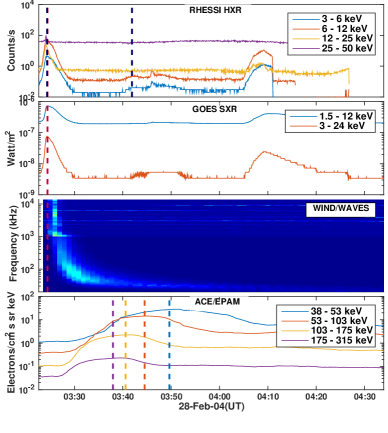
(a)

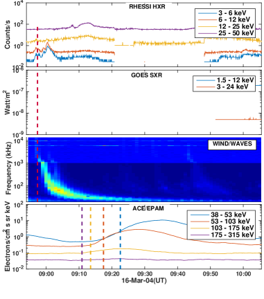
(b)

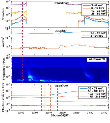
(c)

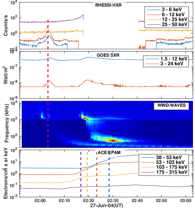
(d)

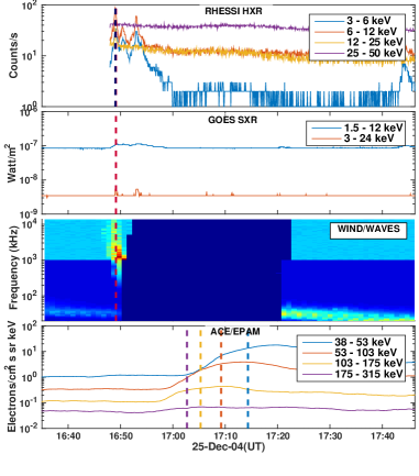
(e)

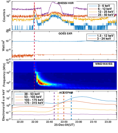
(f)

Figure 1: Stacked plots for each of the six shortlisted events. The top panel shows the corrected RHESSI HXR photon counts. The dark red dashed line depicts the quantity $t_{sun}$, which corresponds to the peak of the HXR emission in the 12-25 keV channel. The dark blue dashed line depicts the timing of the HXR flare from the RHESSI flare list, where available. Since our shortlisted events are very weak, only two events are found in the RHESSI flare list. The second panel shows the GOES SXR flux. The third panel is the WIND/WAVES dynamic spectrum, showing the interplanetary type III burst associated with each event. The bottom panel shows the time evolution of the electron flux in the four ACE/EPAM energy channels. The thick dashed lines correspond to the expected arrival times of the electrons in the different energy channels, assuming that they are released at $t_{sun}$ and travel a distance of 1 AU.

Table 1: Impulsive electron events detected in-situ at 1 AU: first shortlist

Event Date	Onset at	Onset at	GOES flux	Type III onset at	SEP onset
	Sun ($t_{sun}$)	GOES	level	WIND/WAVES	at ACE-DE4
	(UT)	(UT)		(UT)	(UT)
Feb 28,2004*	03.24	03.24	B6.6	03.25	03.36
Mar 16,2004*	08.56	no-data	C0.1	08.57	09.12
June 26,2004	20.50	nil	B2.1	20.51	21.13
June 26,2004*	22.50	22.50	B2.2	22.51	23.02
June 27,2004*	02.03	02.02	B1.1	02.03	02.17
June 27,2004	04.59	05.01	B1.1	05.01	05.19
June 27,2004	13.02	13.01	C0.0	13.02	13.21
June 27,2004	14.59	nil	B1.1	15.01	15.26
June 27,2004	17.43	nil	B1.1	17.43	18.10
Dec 25,2004*	16.49	16.50	B0.0	16.49	17.03
Dec 25,2004*	22.29	22.29	B0.1	22.29	22.43
Mar 16,2005	23.03	23.02	B1.3	23.02	23.19
Jan 13, 2007	15.10	15.11	B2.2	15.12	15.21
Feb 18, 2010	18.58	18.56	A9.1	18.59	19.14
Mar 28, 2014	20.57	20.58	C0.0	20.58	21.18
Jan 20, 2015	09.48	09.49	B9.1	09.50	10.05
May 14,2015	05.08	05.10	C0.6	05.10	05.23
May 14,2015	07.28	07.29	C1.0	07.29	07.40

• Events in the final shortlist.

2.3 Shortlist 2: Association with IP type III bursts

We would expect the escaping electrons to excite interplanetary type III bursts. We use data from the WAVES RAD1 (20 - 1040 kHz) and RAD2 (1.075 - 13.825 MHz) detectors aboard the WIND spacecraft to search for interplanetary type III bursts associated with the impulsive electron events detected by ACE/EPAM. We find that all the events have an associated IP type III burst with onset times within a minute of the onset at the Sun $t_{sun}$. This indicates that electron injection into the interplanetary space happened during the flaring process and any delay at ACE/EPAM is purely due to propagation effects. This is unlike delayed SEP events, in which electron injection happens tens of minutes after the flaring process.The column titled “Onset at WAVES” in Table 1 indicates the time of onset of the IP type III burst in the WIND/WAVES RAD2 receiver.

2.4 Shortlist 3: Association with HXR emission

We further require that the events we analyze have enough HXR photon counts for carrying out spectroscopic and imaging anaylsis using RHESSI data. We require that the the RHESSI signatures are located near the west limb, which would enable better magnetic connectivity to the Earth for escaping electrons (Figure 3 and Table 2). This defines our third and final shortlist, comprising 6 events, which are listed in Table 2. We note that all but one of the events (Feb 28 2004) have very few photon counts above 35 keV. Since most of the events are very weak compared to standard RHESSI flares only two of them have been included in the RHESSI flare list (${\rm http://hesperia.gsfc.nasa.gov/hessidata/dbase/hessi_{-}flare_{-}list.txt}$).

3 Data Analysis

The general picture we have in mind is as follows: electrons are accelerated in the corona during episodes of magnetic reconnection. Some of these accelerated electrons propagate downwards towards the Sun and produce HXR emission via the thick-target bremsstrahlung process. Some find access to open magnetic field lines, manifesting as impulsive electron events detected in-situ by ACE/EPAM and producing interplanetary type III bursts on the way.

The stacked plots shown in figure 2.2 depict the observational signatures of this chain of events. The red dashed line denotes the event onset time at the Sun ($t_{sun}$). The topmost panel depicts the HXR photon counts measured by the RHESSI detectors. The second panel shows the GOES soft Xray flux. There is a small enhancement of the GOES soft Xray flux for each event, although the level is $<$ C1. The low frequency radio dynamic spectrum recorded by WIND/WAVES is depicted in the third panel; it shows interplanetary type III bursts due to the electrons escaping from the coronal acceleration site. The bottom panel shows the electron flux measured in-situ by ACE/EPAM. The dashed lines show expected arrival times for the different energy channels computed according to Eq 1.

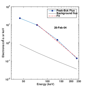
(a)

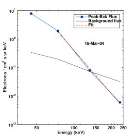
(b)

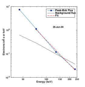
(c)

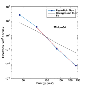
(d)

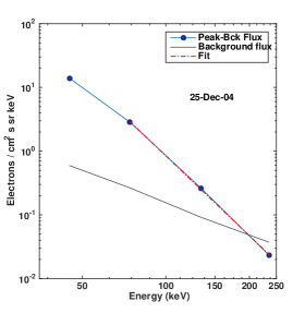
(e)

(f)

Figure 2: Fits to the ACE/EPAM electron data for each of the six shortlisted events. The background spectrum was subtracted to the from the spectrum at the event peak. We observe a break in the spectrum for all the events at 74 keV. We fit a power law to the spectrum above the break. This is depicted by the thick blue line in the graphs. Results are tabulated in Table 2.

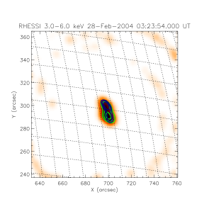
(a)

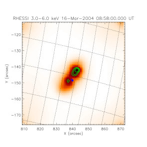
(b)

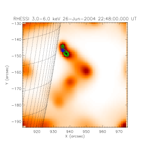
(c)

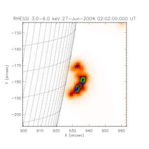
(d)

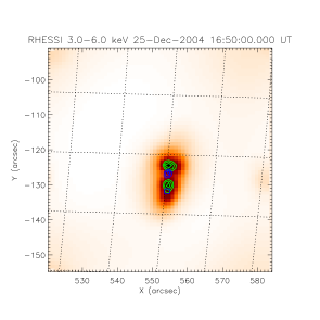
(e)

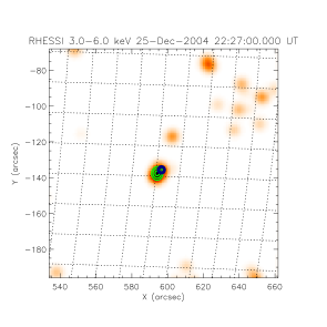
(f)

Figure 3: HXR images using the Pixon algorithm in the OSPEX/RHESSI routine for the six events in our final shortlist. The green contours show 70%, 80%, and 90% emission levels in the 3-6 keV band. The blue contours show the 70%, 80% and 90% emission levels in the 6-9 keV band.

3.1 Escaping electrons detected at 1AU

Electrons arriving at 1 AU are recorded in four energy channels between 38 and 315 keV by ACE/EPAM. We use ACE/EPAM 12 second data (Gold et al., 1998). The peak mean energies of the four channels, DE1-4 are 45,74,134 and 235 keV respectively. Based on the flux at the peak of the event recorded at the mean energy of each ACE/EPAM energy channel, the differential energy spectrum of the particles can be represented as,

$$dJ/dE\propto E^{\delta_{1}}$$ (2)

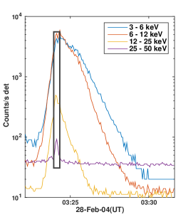
(a)

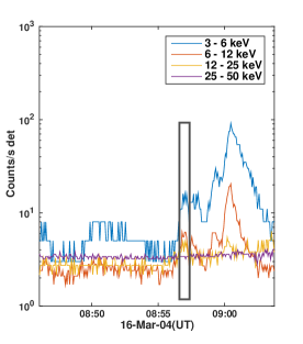
(b)

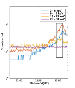
(c)

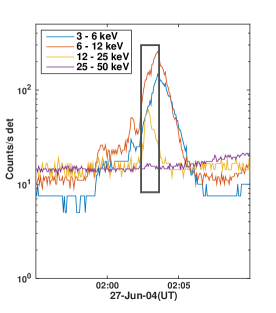
(d)

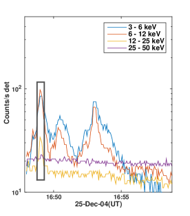
(e)

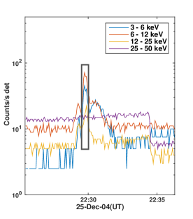
(f)

Figure 4: The HXR lightcurves for each of the six shortlisted events. The energy bands used for plotting the graph were 3-6 keV,6-12 keV, 12-25 keV, 25-50 keV, 50-100 keV. Due to weak nature of the events, there is little data in the highest energy band for most events. The shaded recatangle show the time strips used to generate the photon spectrum used in OSPEX.

Table 2: Final shortlist and spectral parameters

Date	RHESSI Peak	Flare Position	$\gamma$	$\delta_{1AU}$	$\delta_{hxr}$
	Time(UT)	Heliocentric
		x,y(arcsec)
Feb 28,2004	03.24	697, 301	3.69	4.14	4.89
Mar 16,2004	08:56	841, -144	4.38	5.25	5.54
June 26,2004	22.50	943, -162	4.66	5.45	5.80
June 27,2004	02.03	931, -176	4.24	5.10	5.13
Dec 25,2004	16.49	552, -123	3.25	4.39	4.43
Dec 25,2004	22.29	598, -132	3.10	4.12	4.06

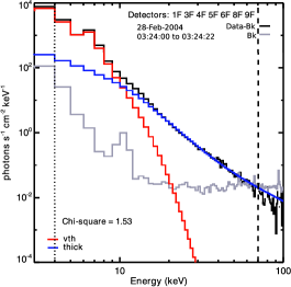
(a)

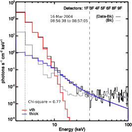
(b)

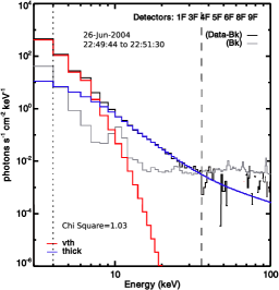
(c)

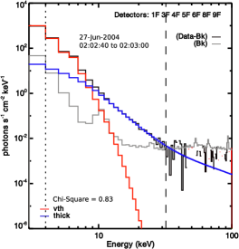
(d)

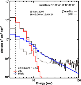
(e)

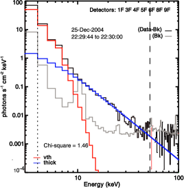
(f)

Figure 5: The OSPEX spectral fits for each of the six shortlisted events. RHESSI front detectors 1,3,4,5,6,8,9 were used to accumulate the data. Since the events are weak, we restrict the fit to energy ranges which have counts above the background emission levels. The dashed vertical lines indicate the range of energies used for the fit. A photon spectral index $\gamma$ is obtained through a broken power law fit (not shown). The emission measure and thermal temperature are obtained from variable thermal function fit. The thick target fit gives the hxr producing electron spectral indice $\delta_{hxr}$. Results are tabulated in Table 2.

where $\delta_{1}$ is the spectral index of electrons escaping from the coronal acceleration site and detected in-situ at 1 AU by ACE/EPAM. This is distinct from the spectral index $\delta_{\rm hxr}$ of the HXR producing electrons, which is estimated in § 3.2. The values of these indices for each event are summarized in Table 2. For a given event, one would expect that $\delta_{1}$ and $\delta_{\rm hxr}$ be similar to each other, if the electrons propagate in a reasonably scatter-free manner from the Sun to the Earth.

The fit to the spectra of electrons detected in-situ at 1 AU by ACE/EPAM for all the events are shown in Fig 2. The fits are constructed using the peak count in each energy bin. All the events typically show a break in the spectrum at around 74 keV (Figure 2). By contrast, the break energy for larger flares tends to be around 48 keV (e.g., Krucker et al. (2007)). The break energy in the spectrum presumably indicates the energy above which wave-particle interactions are unimportant (Kontar & Reid, 2009). We note that Krucker et al. (2007) used WIND/3DP data for their analysis. Of the events in our final shortlist, four have reliable WIND/3DP data. The break energy for these events as ascertained from WIND/3DP data is $\approx$ 66 keV, which corresponds to the mean energy of the corresponding channel on that instrument.

3.1.1 Number flux, power and energy in Escaping electrons

Having fitted the differential electron flux at 1 AU $F(E)$ (${\rm electrons\,s^{-1}\,sr^{-1}\,keV^{-1}\,cm^{-2}}$) to a power law of the form $F(E)=F_{0}(E_{0}/E)^{\delta_{1}}$, (Table 2) it follows that the flux of electrons above $E_{0}$ is

$$\int_{E_{0}}^{\infty}F(E)dE=\frac{F_{0}E_{0}}{(\delta_{1}-1)}\,\,\,{\rm electrons\,s^{-1}\,sr^{-1}\,cm^{-2}}\,.$$ (3)

The quantity $E_{0}$ is the break energy in ACE/EPAM data (typically around 74 keV) above which the power law fit is valid and $F_{0}$ is the peak differential energy flux at $E_{0}$. The number of escaping electrons per second above $E_{0}$ detected by ACE/EPAM at 1 AU and the power carried by them are given by

$$\Omega(1AU)^{2}\int_{E_{0}}^{\infty}F(E)dE=\Omega(1AU)^{2}\frac{F_{0}E_{0}}{(\delta_{1}-1)}\,\,\,{\rm s^{-1}}\,,\,\,\,{\rm and}$$

$$\noindent\Omega(1AU)^{2}\int_{E_{0}}^{\infty}EF(E)dE=\Omega(1AU)^{2}\frac{F_{0}E_{0}^{2}}{(\delta_{1}-2)}\,\,\,\,{\rm erg\,s^{-1}}$$ (4)

respectively, where $\Omega$ is the solid angle spread of the electrons at 1 AU, which we take to correspond to a cone of 30^∘ (Lin, 1974; Krucker et al., 2007). The factor of $(1AU)^{2}$ arises from assuming that the electrons are spread uniformly over a sphere of radius 1 AU. Multiplying the expression for power by the duration of the impulsive electron event at 1 AU yields the energy carried by the escaping electrons. The power (${\rm erg\,s^{-1}}$) and energy (ergs) for each of our shortlisted electron spikes detected at 1 AU are listed in Table 5.

3.2 HXR producing electrons

The RHESSI HXR photon spectrum for each event was analysed using SSW/OSPEX. The assumed HXR photon spectrum consists of a thermal core and a long non-thermal tail. The event duration in the lowest available energy channel (which has a reasonable number of counts) was used as integration time for computing the spectra. We applied a broken power law fit to the non-thermal tail (Figure 5), with a variable thermal function for the thermal core at low energies. The background spectrum dominates the event spectrum above 35 keV for most of the events. We perform these fits only for energies with photon counts above the background. The photon spectral indices $\gamma$ are listed in Table 2. We note that break energies for large flares are $\sim$ 45 keV (Krucker et al., 2007; Oka et al., 2013). The fit for all the events are shown in Figure 5 . The HXR spectral indices for all the events are shown in Table 2 . Assuming the injected electron spectrum in the coronal acceleration site is same as the interplanetary electron spectrum, Datlowe & Lin (1973) noted that a thick target model for HXR emission gives $\delta_{1}=\gamma+1$ while a thin target one gives $\delta_{1}=\gamma-1$.

We find that the photon spectral index $\gamma$ is related to the electron spectral index $\delta_{1}$ observed at 1 AU via $\delta_{1}=\gamma+1$ with a correlation coefficient of 0.86 (Figure 7a). Our finding that $\delta_{1}=\gamma+1$ thus suggests that the HXR emission is produced via the thick target bremsstrahlung process.

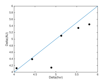
(a) Delta indices

Figure 6: A scatterplot between $\delta_{1AU}$ and $\delta_{hxr}$. The two indices are linearly related with a correlation coefficient of 0.91

We therefore employ a thick target model, with a isothermal function for the thermal component. We require that the thermal temperature and emission measure of the variable thermal function remain constant from the previous fit for estimating the photon spectral index.

The thick target function gives the integrated electron flux at the HXR production site, injected electron spectrum and low energy cutoffs. It also inverts the photon spectrum to give a broken power law electron spectrum, with the break occurring at the injection energy. The spectral index below the injection energy is denoted by $\delta_{hxr}$, and is tabulated in Table 2. Figure 6 shows a scatter plot of $\delta_{hxr}$ and $\delta_{1}$. The results of our analysis in Sec 3.1 reveal that the spectral index of the HXR producing electrons and that of the electrons detected at 1 AU are not very different. They exhibit a linear correlation with a coefficient of 0.91. This implies that the electron population emitting HXR radiation and the one detected at 1 AU have a common origin in the coronal acceleration region.

Table 3: Number of HXR producing and escaping Electrons

Date	Number of	Number of	Escaping fraction
	hxr producing	escaping	$\eta=(N_{esc}/N_{hxr})\%$
	electrons$N_{hxr}$	electrons$N_{esc}$
	(>74 keV)	(>74 keV)
Feb 28,2004	1.82$\times 10^{33}$	1.16$\times 10^{32}$	6.36
Mar 16,2004	3.60$\times 10^{30}$	5.35$\times 10^{30}$	148.3
June 26,2004	2.31$\times 10^{31}$	1.07$\times 10^{30}$	4.64
June 27,2004	5.21$\times 10^{31}$	6.03$\times 10^{31}$	115.7
Dec 25,2004	1.89$\times 10^{32}$	3.31$\times 10^{31}$	17.44
Dec 25,2004	8.57$\times 10^{31}$	3.65$\times 10^{31}$	42.62

Table 4: Fit Parameters of the Events

Date	Thermal	Emission	Energy	Density of	Volume
	Temperature$(MK)$	Measure$(10^{46}cm^{-3})$	Cutoff $(keV)$	thermal plasma$(10^{10}cm^{-3})$	($10^{25}cm^{3}$)
Feb 28,2004	13.53	9.27	14.4	4.50	5.05
Mar 16,2004	11.08	0.95	12.34	3.33	0.86
June 26,2004	11.32	1.08	9.38	2.10	2.43
June 27,2004	11.50	1.73	10.01	2.34	3.15
Dec 25,2004	10.05	0.68	11.2	2.22	1.39
Dec 25,2004	10.23	0.13	10.89	0.84	1.78

3.2.1 Number flux, power and energy in HXR producing electrons

The number of electrons per second involved in producing the HXR emission ($\dot{N}_{>E_{c}}$) is computed for each event by the SSW/OSPEX thick target emission model. This procedure also yields the cutoff energy $E_{c}$ and the power law index $\delta_{\rm HXR}$ of the electron spectrum above $E_{c}$. Since the number of electrons escaped and detected at 1 AU, were estimated only above 74 keV, we scale the corresponding number of HXR electrons above 74 keV using equation Eq 5.

$$\dot{N}_{>74keV}=\dot{N}_{>E_{c}}\bigg{(}\frac{E_{c}}{74}\bigg{)}^{\delta_{hxr}-1}$$ (5)

Following the same logic used in writing Eq 3.1.1, the power in the HXR emitting electrons above $E_{c}$ is given by

$$P=(74keV)\dot{N}_{>74keV}\frac{\delta_{hxr}-1}{\delta_{hxr}-2}$$ (6)

Multiplying this quantity with the duration of the HXR emission yields the total energy in the nonthermal HXR producing electrons. These quantities are listed in Table 3 for each of our shortlisted events. The ratio ($\eta$) of the escaping electrons to the HXR producing electrons ranges from $\approx$ 6 % to over 100 %. By comparison, $\eta$ for the larger flares reported in Krucker et al. (2007) is typically only 0.2 %. Some of these results are graphically depicted in figure 7. Figure 7a shows the plot of $\delta_{1AU}$, the energy spectral index of escaping electrons detected in-situ at 1AU and the $\gamma$, the photon spectral index. The spectral indices follow a functional relation closely resembling a thick target bremmstrahlung process. For big flares, this relation is not as pronounced Krucker et al. (2007). A plot of number of HXR producing electrons at the acceleration site and the number of escaping electrons detected at 1AU is plotted in Figure 7b. Comparing this graph with that for big flares (eg: Fig 3b, Krucker et al. (2007)), we note that the fraction of escaping electrons for the weak events discussed in this paper is much larger.

3.2.2 Thermal HXR emission

We next estimate the energy content of the thermal HXR emission generated by the accelerated electrons. The thermal energy $U_{th}$ is given by

$$U_{th}=3k_{B}T\sqrt{\epsilon_{em}V}$$ (7)

where $\epsilon_{em}$ is the emission measure and $V$ is the volume of the emission region. The emission measure is a product of the electron density $n_{e}$ , ambient plasma density $n_{i}$ and the volume $V$. The emission measure and temperature is determined using the thermal fit to the photon spectrum. The area A of the emission region was estimated by first fitting a Guassian to the 70 % flux contour levels of the RHESSI image We used the Pixon algorithm which gives a sharper image as compared to the Clean algorithm (Dennis & Pernak, 2009).The volume was computed using the formula

$$V=A^{3/2}$$ (8)

Using this method we found the volume to be $\sim 10^{25}{\rm cm}^{3}$ which is very low compared to volumes usually cited for radio noise storms or large flares (Subramanian & Becker, 2006; Krucker et al., 2007; Lin & Hudson, 1971). This value is similar to values for the smallest of microflares reported by Hannah et al. (2008). For each event, we derive an upper limit on the electron density using the emission measure, which we derived by applying a thermal fit to the photon spectra. The emission measure was found to be around $10^{45}{\rm cm}^{-3}$ for all events. The ambient plasma density $n_{i}$ is calculated using the thick target model; it turns out to be $\sim 10^{10}{\rm cm}^{-3}$ for most events. Using these values for $n_{i}$, V,and the emission measure we found typical background electron densities of $\sim 10^{10}{\rm cm}^{-3}$ (Table 4). These numbers are around an order of magnitude larger than those typically found for cold/tenuous flares (Fleishman et al., 2011). The total thermal HXR energy thus calculated was found be $\sim 10^{28}$ ergs (Table 5).

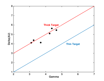
(a) Thick target relation of spectral indices

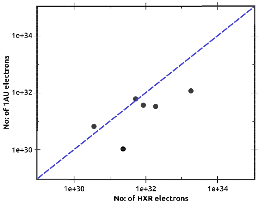
(b) Spectral dependence of $\gamma$ and $\delta_{1}$

Figure 7: The top panel shows a scatterplot of the photon spectral index $\gamma$ plotted against $\delta_{1}$ (Table 2). We note that the data points fit $\delta_{1}=\gamma+1$ with a correlation coefficient of 0.94. This indicates that the HXR radiation is most likely produced via thick target emission. The bottom panel shows a scatterplot of the total number of $>74$ keV electrons detected at 1AU plotted against the number of $>74$ keV electrons involved in HXR emission.

Table 5: Energy chracteristics of Events

Date	Energy in	Energy contained	Energy carried away	Power	Power
	thermal HXR emission	in HXR electrons	by escaping electrons	in HXR electrons	in escaping electrons
	(ergs)	(ergs)	(ergs)	(ergs/s)	(ergs/s)
Feb 28, 2004	1.06$\times 10^{28}$	5.79$\times 10^{26}$	3.38$\times 10^{25}$	1.69$\times 10^{24}$	9.07$\times 10^{21}$
March 16,2004	1.19$\times 10^{27}$	1.69$\times 10^{24}$	4.94$\times 10^{24}$	1.18$\times 10^{23}$	8.78$\times 10^{20}$
June 26,2004	2.40$\times 10^{27}$	9.94$\times 10^{24}$	1.05 $\times 10^{23}$	4.17$\times 10^{23}$	4.89$\times 10^{21}$
June 27,2004	3.51$\times 10^{27}$	1.18$\times 10^{25}$	9.55$\times 10^{24}$	1.15$\times 10^{23}$	5.39$\times 10^{21}$
Dec 25,2004	1.28$\times 10^{27}$	2.16$\times 10^{25}$	7.32$\times 10^{24}$	1.08$\times 10^{23}$	3.15$\times 10^{21}$
Dec 25,2004	6.48$\times 10^{26}$	1.02$\times 10^{25}$	6.05$\times 10^{24}$	3.87$\times 10^{23}$	3.26$\times 10^{21}$

4 Summary and Conclusions

4.1 Summary

We have investigated the energy budgets involved in small electron acceleration events in the solar corona. We envisage a scenario where these (small) acceleration events occur relatively high in the corona. Subsequently, some of the accelerated electrons travel downwards and encounter the relatively dense chromospheric layers, resulting in the observed HXR emission via thick target bremsstrahlung. Some of the accelerated electrons escape outwards from the corona, travelling towards the Earth along the Parker spiral, and are detected in-situ at 1 AU as impulsive electron events by the ACE/EPAM detectors. We concentrate on events that give rise to faint, but observable HXR emission near the west limb, and are also associated with IP type III bursts and impulsive electron spikes observed in-situ at 1 AU. These events are not associated with soft Xray flares $>C1$ or with CMEs. These selection criteria yield 6 events between 2004 and 2015. We use RHESSI data for HXR emission and analyze it using the standard RHESSI/OSPEX routines. For each event, we investigate the acceleration energy budget for the electrons that produce the observed HXR emission as well as the ones that escape out of the corona to reach the Earth.

4.2 Conclusions

In some respects (such as the lack of appreciable soft X-ray emission and the relatively low background thermal electron densities) the events we have shortlisted are similar to the cold and tenuous flares reported by (Fleishman et al., 2011, 2016) . We find that the electrons escaping from the acceleration site and detected at 1.2 AU have a power law law index ($\delta_{1}$) that is similar to the ones which produce the HXR emission ($\delta_{HXR}$). This suggests that the escaping electrons and the HXR producing electrons arise from the same population that was accelerated in the corona. The escaping electrons detected at 1 AU in the DE 4 channel take $\approx$ 14 minutes to travel from the Sun to the Earth, which suggests that scattering effects are not important (see Figure 2.2).

We compute the number, power and total energy in the nonthermal electron populations producing the 1 AU electron spikes and the corresponding HXR emission using the prescriptions outlined in § 3.1.1 and 3.2.1. Our main results are:

• The ratio of the number of escaping electrons (that are detected in-situ at 1 AU by ACE/EPAM) to the number of (downward precipitating) HXR producing electrons ranges from 6 % to a number as large as 148 % (Table 3) . By comparison, Krucker et al. (2007), who analyzed much larger (typically M class) flares, found a ratio of $\approx 0.2\%$. On the other hand, based on simulations,Wang et al. (2016) estimate that, in the quiet Sun, the ratio of electrons propagating outwards to form the solar wind superhalo to those that could potentially propagate downwards and produce HXR emission can be as high as 30 %.

• The total energy in the electron spikes detected at 1 AU ranges from $\approx 10^{23}$ to $10^{25}$ erg, while that in the nonthermal electron population producing the corresponding HXR events is $\approx 10^{24}$ – $10^{26}$ erg (Table 5). On the other hand, the energy contained in thermal HXR emission is found to range from $10^{26}$-$10^{28}$ erg.

Our analysis yields insights pertaining to nonthermal electron acceleration in very small events, which can serve as a useful guide to understanding the feasibility of direct detections of nanoflares.Our results are also relevant to recent theories concerning particle acceleration in the turbulent solar corona. Astrophysical plasmas are expected to be generically turbulent; the solar corona and the solar wind are archetypal examples. The presence of turbulence is expected to make the reconnection rate independent of microphysical (anomalous) resistivity and engender fast reconnection (Lazarian & Vishniac (1999); Lazarian et al. (2015) and references therein). Alfvenic scattering centres in the vicinity of the turbulent reconnection sites are expected to aid in accelerating electrons (Vlahos et al., 2016). Our results can constrain the parameters of such turbulence-aided acceleration scenarios. For instance, the spectral slope of the high energy tail of the electrons detected in-situ at 1 AU (which is fairly similar to that of the electrons producing HXR emission) can be used as a guide for determining the ratio of the acceleration timescale to the escape timescale.

References

- Arzner & Vlahos (2004) Arzner K., Vlahos L., 2004, The Astrophysical Journal, 605, L69
- Aschwanden (2012) Aschwanden M. J., 2012, Space Science Reviews, 171, 3
- Aschwanden et al. (2017) Aschwanden M. J., et al., 2017, The Astrophysical Journal, 836, 17
- Barnes et al. (2016) Barnes W. T., Cargill P. J., Bradshaw S. J., 2016, The Astrophysical Journal, 829, 31
- Beltran et al. (2015) Beltran S. D. T., Cutchin S., White S., 2015, Solar Physics, 290, 2423
- Dahlin et al. (2015) Dahlin J. T., Drake J. F., Swisdak M., 2015, Physics of Plasmas, 22, 100704
- Datlowe & Lin (1973) Datlowe D. W., Lin R. P., 1973, Solar Physics, 32, 459
- Dennis & Pernak (2009) Dennis B. R., Pernak R. L., 2009, ApJ, 698, 2131
- Fleishman et al. (2011) Fleishman G. D., Kontar E. P., Nita G. M., Gary D. E., 2011, The Astrophysical Journal, 731, L19
- Fleishman et al. (2016) Fleishman G. D., Pal'shin V. D., Meshalkina N., Lysenko A. L., Kashapova L. K., Altyntsev A. T., 2016, The Astrophysical Journal, 822, 71
- Gold et al. (1998) Gold R., et al., 1998, Space Science Reviews, 86, 541
- Hannah et al. (2008) Hannah I. G., Christe S., Krucker S., Hurford G. J., Hudson H. S., Lin R. P., 2008, The Astrophysical Journal, 677, 704
- Holman et al. (2011) Holman G. D., et al., 2011, Space Science Reviews, 159, 107
- Joulin et al. (2016) Joulin V., Buchlin E., Solomon J., Guennou C., 2016, Astronomy & Astrophysics, 591, A148
- Klassen et al. (2012) Klassen A., Gómez-Herrero R., Heber B., Kartavykh Y., Dröge W., Klein K.-L., 2012, Astronomy & Astrophysics, 542, A28
- Klimchuk (2015) Klimchuk J. A., 2015, Philosophical Transactions of the Royal Society A: Mathematical, Physical and Engineering Sciences, 373, 20140256
- Kontar & Reid (2009) Kontar E. P., Reid H. A. S., 2009, The Astrophysical Journal, 695, L140
- Kontar et al. (2011) Kontar E. P., et al., 2011, Space Science Reviews, 159, 301
- Kontar et al. (2017) Kontar E., Perez J., Harra L., Kuznetsov A., Emslie A., Jeffrey N., Bian N., Dennis B., 2017, Physical Review Letters, 118
- Krucker et al. (1999) Krucker S., Larson D. E., Lin R. P., Thompson B. J., 1999, The Astrophysical Journal, 519, 864
- Krucker et al. (2007) Krucker S., Kontar E. P., Christe S., Lin R. P., 2007, ApJ, 663, L109
- Krupar et al. (2014) Krupar V., et al., 2014, Solar Physics, 289, 3121
- Krupar et al. (2015) Krupar V., Kontar E. P., Soucek J., Santolik O., Maksimovic M., Kruparova O., 2015, Astronomy & Astrophysics, 580, A137
- Kumar & Bhattacharyya (2016) Kumar S., Bhattacharyya R., 2016, Physics of Plasmas, 23, 044501
- Kumar et al. (2015) Kumar S., Bhattacharyya R., Smolarkiewicz P. K., 2015, Physics of Plasmas, 22, 082903
- Lazarian & Vishniac (1999) Lazarian A., Vishniac E. T., 1999, The Astrophysical Journal, 517, 700
- Lazarian et al. (2015) Lazarian A., Eyink G., Vishniac E., Kowal G., 2015, Philosophical Transactions of the Royal Society A: Mathematical, Physical and Engineering Sciences, 373, 20140144
- Lin (1974) Lin R., 1974, Space Science Reviews, 16
- Lin & Hudson (1971) Lin R. P., Hudson H. S., 1971, Sol. Phys., 17, 412
- Mercier & Trottet (1997) Mercier C., Trottet G., 1997, The Astrophysical Journal, 474, L65
- Miller et al. (1997) Miller J. A., et al., 1997, Journal of Geophysical Research, 102, 14631
- Oka et al. (2013) Oka M., Ishikawa S., Saint-Hilaire P., Krucker S., Lin R. P., 2013, ApJ, 764, 6
- Parker (1988) Parker E. N., 1988, The Astrophysical Journal, 330, 474
- Potter et al. (1980) Potter D. W., Lin R. P., Anderson K. A., 1980, The Astrophysical Journal, 236, L97
- Ramesh et al. (2012) Ramesh R., Raja K. S., Kathiravan C., Narayanan A. S., 2012, The Astrophysical Journal, 762, 89
- Saint-Hilaire et al. (2012) Saint-Hilaire P., Vilmer N., Kerdraon A., 2012, The Astrophysical Journal, 762, 60
- Simnett (2005) Simnett G. M., 2005, Solar Physics, 229, 213
- Simnett et al. (2002) Simnett G. M., Roelof E. C., Haggerty D. K., 2002, The Astrophysical Journal, 579, 854
- Subramanian & Becker (2006) Subramanian P., Becker P. A., 2006, Sol. Phys., 237, 185
- Testa et al. (2013) Testa P., et al., 2013, The Astrophysical Journal, 770, L1
- Vilmer (2012) Vilmer N., 2012, Philosophical Transactions of the Royal Society A: Mathematical, Physical and Engineering Sciences, 370, 3241
- Vlahos et al. (2016) Vlahos L., Pisokas T., Isliker H., Tsiolis V., Anastasiadis A., 2016, ApJ, 827, L3
- Wang et al. (2016) Wang W., Wang L., Krucker S., Hannah I., 2016, Solar Physics, 291, 1357
- Zharkova et al. (2011) Zharkova V. V., et al., 2011, Space Science Reviews, 159, 357