NIKHEF/2017-25 Edinburgh 2017/10 QMUL-PH-17-07 ARC-17-03

Universality of next-to-leading power threshold effects for colourless final states in hadronic collisions

V. Del Duca^1,2, E. Laenen^3,4,5, L. Magnea⁶, L. Vernazza⁷, C. D. White⁸

¹ETH Zurich, Institut fur theoretische Physik, Wolfgang-Paulistr. 27, 8093, Zurich, Switzerland

²INFN Laboratori Nazionali di Frascati, 00044 Frascati (Roma), Italy

³Nikhef, Science Park 105, NL–1098 XG Amsterdam, The Netherlands

⁴ITFA, University of Amsterdam, Science Park 904, Amsterdam, The Netherlands

⁵ITF, Utrecht University, Leuvenlaan 4, Utrecht, The Netherlands

⁶Dipartimento di Fisica and Arnold-Regge Center, Università di Torino,
and INFN, Sezione di Torino, Via P. Giuria 1, I-10125 Torino, Italy

⁷Higgs Centre for Theoretical Physics, School of Physics and Astronomy, The University of Edinburgh, Edinburgh EH9 3JZ, Scotland, UK

⁸Centre for Research in String Theory, School of Physics and Astronomy, Queen Mary University of London, 327 Mile End Road, London E1 4NS, UK

We consider the production of an arbitrary number of colour-singlet particles near partonic threshold, and show that next-to-leading order cross sections for this class of processes have a simple universal form at next-to-leading power (NLP) in the energy of the emitted gluon radiation. Our analysis relies on a recently derived factorisation formula for NLP threshold effects at amplitude level, and therefore applies both if the leading-order process is tree-level and if it is loop-induced. It holds for differential distributions as well. The results can furthermore be seen as applications of recently derived next-to-soft theorems for gauge theory amplitudes. We use our universal expression to re-derive known results for the production of up to three Higgs bosons at NLO in the large top mass limit, and for the hadro-production of a pair of electroweak gauge bosons. Finally, we present new analytic results for Higgs boson pair production at NLO and NLP, with exact top-mass dependence.

1 Introduction

The remarkable experimental precision and high statistics offered by current and future colliders necessitates the calculation of high-order effects in QCD perturbation theory for processes of increasing complexity. The calculation of next-to-leading order (NLO) QCD corrections has reached the stage where automated tools are being used and multi-jet production rates are evaluated (see, for example [1]). Attention then focuses on QCD corrections at NNLO or above, and on the inclusion of higher-order electroweak effects. In this context, processes which are induced by loop effects present special difficulties: typically, the leading order contribution involves a loop containing heavy particles, such as top quarks or electroweak vector bosons, and is often computed in the context of an effective field theory. NLO QCD corrections with exact dependence on the heavy particle masses then involve intricate two-loop calculations: for multi-particle final states, these corrections are not known, and even for two-particle final states they are typically only known approximately, or in some cases numerically. Clearly, in all these cases it is desirable, where possible, to improve upon existing results by providing analytic information. Even partial information can be useful, since it can be used, for example, to speed up numerical codes, and also to provide additional consistency checks.

In this paper, we consider the production of a generic colour-singlet final state in hadronic collisions, and we study the effects of additional gluon radiation near partonic threshold, where emitted gluons have a low energy or transverse momentum with respect to the incoming partons. In such cases, one commonly defines a dimensionless threshold variable $\xi$, vanishing at the threshold, and it is well known that the corresponding differential cross section has the generic form

$$\frac{d\sigma}{d\xi}\,=\,K_{\rm ew}\left(4\pi\alpha_{s}\right)^{n_{0}}\sum_{n=0}^{\infty}\left(\frac{\alpha_{s}}{\pi}\right)^{n}\sum_{m=0}^{2n-1}\left[\,c_{nm}^{(-1)}\left(\frac{\log^{m}\xi}{\xi}\right)_{+}+\,c_{n}^{(\delta)}\,\delta(\xi)+\,c_{nm}^{(0)}\,\log^{m}\xi+\ldots\,\right],$$ (1.1)

where the overall factor is associated with the leading-order cross section: for loop-induced processes, this may be proportional to a power of the strong coupling, as indicated, while $K_{\rm ew}$ contains electroweak couplings. The first two sets of terms on the right-hand side of Eq. (1.1) originate from soft and collinear radiation (real or virtual), and correspond to the leading power in the threshold variable, and to corrections localised at the threshold, respectively. These contributions are known to have a universal (process-independent) form, that permits their resummation to all orders in perturbation theory. This resummation is well understood and widely applied, and can be performed within a variety of approaches (see for example [2, 3, 4, 5, 6, 7, 8, 9, 10, 11]). Even without a full resummation, a fixed order evaluation of these terms can be useful in estimating higher-order corrections to the cross-section, when these are not known (see for example [12] for a review).

The third set of terms on the right-hand side of Eq. (1.1) defines next-to-leading power (NLP) contributions in the threshold variable, roughly corresponding to gluon radiation that can be next-to-soft or collinear. Although power-suppressed, these terms are still singular as $\xi\rightarrow 0$, and can be numerically significant: for example, they contribute significantly to the theoretical uncertainty for Higgs boson production in the gluon fusion channel [13], and their numerical impact has been explicitly confirmed by the recent calculation of this process at N³LO [14, 15, 16, 17, 18]. A full, generally applicable resummation prescription for NLP contributions is not presently known, even in the relatively simple case of parton annihilation into electroweak final states: the problem has been intensively studied in recent years, and partial progress has been made using a variety of methods [19, 20, 21, 22, 23, 24, 25, 26, 27, 28, 29, 30, 31, 32, 33, 34, 35, 36, 37, 38, 39], buiding upon the earlier work of [40, 41, 42]. Even without a full resummation, however, knowledge of NLP contributions at fixed order can provide useful analytic information where this is missing, as well as furnishing improved approximations for unknown higher-order cross sections. This is especially true if one can derive universal properties of NLP contributions, applicable at a given order for a broad class of processes.

In this paper, we examine the universal properties of NLP radiation in the hadro-production of an arbitrary number of colour-singlet particles at NLO. We will prove that the NLO cross-section for this class of processes can be written in terms of the leading-order cross-section with shifted kinematics, convolved with a simple universal $K$-factor. More precisely, we find that the $K$-factor does not depend on the spin of the emitting parton, and depends on the color representation only through a trivial replacement of colour factors. Our starting point will be a factorisation formula for NLP effects at amplitude level recently derived in Refs. [23, 24], which expresses the effect of adding an additional gluon to an arbitrary hard process with an electroweak final state in terms of universal functions. Our results provide a useful testing ground for this formula, and an examination of its simpler consequences, aside from its role as a basis for resummation. Furthermore, our results have more practical consequences, providing an analytic approximation to the NLO cross section for a number of interesting loop-induced processes for which only limited information is available. Interestingly, the universality of the result extends to differential distributions, provided the shift in LO kinematics is properly understood. From a theoretical point of view, the universality and simplicity of our results at NLO can be seen as a consequence of recently derived next-to-soft theorems [43, 44, 45] for radiative tree-level gauge theory amplitudes: we note however that our factorisation formula is an all-order result, and therefore will yield more general results, once the appropriate ingredients are computed at the relevant orders.

From the point of view of phenomenology, the most interesting applications of our results will concern the production of Higgs bosons in the gluon fusion channel, possibly in association with electroweak gauge bosons. We will however show explicitly that the formalism can be used also with (anti)quark initial states, and compare our results with existing calculations. In the gluon fusion channel, we will begin by showing how known properties of the single Higgs boson cross section emerge as a special case of our result. We next move on to multiple Higgs boson production, which has been the focus of much recent research. Beyond the leading-order result [46], we note that analytic expressions for the cross section are known only in the large top mass limit for Higgs pair production [47, 48] and for triple Higgs boson production [49]. In the case of Higgs pair production, leading order results with full top mass dependence were obtained in refs. [50, 51], and numerical results have recently been presented at NLO [52] (see also [53]); leading power threshold corrections have been considered in Ref. [54], and corrections to the large top mass approximation in Ref. [55]. In the case of triple Higgs boson production, numerical results with full top mass dependence at leading order and for real radiation at NLO were obtained in Ref. [56] and in Ref. [57], respectively. Associated production of electroweak bosons and Higgs bosons in the gluon fusion channel, discussed in Ref. [58], also falls within the scope of our method, although we will not discuss it in detail here.

In this paper, we go beyond previous analytic results for Higgs boson pair production, by providing NLO corrections, up to NLP in the threshold variable, with full top mass dependence. As a further illustration and check, we demonstrate consistency with known results for triple Higgs boson production in the large top mass limit [49], diphoton production [59], and the production of $W^{+}W^{-}$ pairs [60]. These results serve as an illustration of the method: we postpone a detailed phenomenological analysis, as well as applications to triple Higgs production with full top mass dependencce, and to associated production of Higgs bosons with Z bosons, to future work. We note in passing that the present results also provide a strong consistency check on all future NLO analytic computations of loop-induced processes of colour-singlet particles, which of course must agree with the simple factorised expressions we derive at NLP.

The structure of our paper is as follows. In Section 2, we briefly review the next-to-soft factorisation formula of Refs. [23, 24], before describing how it can be extended for use in gluon-induced processes. In Section 3, we derive an explicit expression for the NLO cross-section of a colour-singlet final state in gluon fusion, valid up to NLP level. A similar result for the quark channel is derived in Section 4. In Section 5, we show how known results in single Higgs boson production are reproduced, before examining multiple Higgs boson production in Section 6. Vector boson pair production is considered in Section 7. Finally, we discuss our results and future prospects in Section 8.

2 NLP amplitude factorisation

In this section, we briefly review the results of Refs. [23, 24], which derive a factorisation formula for QCD radiation up to NLP level, and we provide a generalisation of these results to the case of external incoming gluons. Consider an amplitude with two incoming partons of momenta $p_{1}$ and $p_{2}$, and any number $N$ of final state colour singlet particles, with momenta $p_{i}$, $3\leq i\leq N+2$. As described in detail in Ref. [24], any such amplitude may be written in the factorised form

$${\cal A}(\{p_{i}\})\,=\,\tilde{H}\left(\{p_{i}\},n_{1},n_{2}\right)\tilde{\cal S}\left(p_{1},p_{2}\right)\frac{\prod_{k=1}^{2}J(p_{k},n_{k})}{\prod_{k=1}^{2}\tilde{\cal J}(p_{k},n_{k})}\,.$$ (2.1)

Here $\tilde{\cal S}(p_{1},p_{2})$ is a next-to-soft function, dressing the hard interaction with virtual exchanges of (next-to-)soft gluons, which couple to the external partons through the next-to-eikonal Feynman rules described in Refs. [20, 21]. Associated with each hard parton is a jet function $J(p_{i},n_{i})$, which collects collinear singularities, and which depends on an auxiliary vector $n_{i}$. The next-to-eikonal jet $\,\tilde{\cal J}(p_{i},n_{i})$ corrects for the double counting of contributions from gluons which are both (next-to-)soft and collinear, and finally the hard function $\tilde{H}(\{p_{i}\},n_{1},n_{2})$ is defined by matching to the amplitude on the left-hand side of Eq. (2.1), so that all dependence on the auxiliary vectors $\{n_{i}\}$ cancels out. If one ignores the presence of next-to-eikonal Feynman rules, Eq. (2.1) reduces to the well-known soft-collinear factorisation formula, describing the dressing of a given hard interaction process with leading-power soft and collinear radiation (see, for example, [61]). The form of Eq. (2.1), however, is a crucial intermediate step in considering the emission of an additional gluon, of momentum $k^{\mu}$ and colour $a$. Up to NLP in this momentum, the resulting amplitude is given by [24]

$${\cal A}_{\mu}^{\,a}\left(\{p_{i}\},k\right) = \sum_{l=1}^{2}\Bigg{\{}\Bigg{[}\frac{1}{2}\,\frac{\tilde{\cal S}_{\mu}^{\,a}\left(p_{1},p_{2},k\right)}{\tilde{\cal S}(p_{1},p_{2})}+g_{s}\,{\bf T}_{l}^{a}\,G^{\nu}_{l,\mu}\,\frac{\partial}{\partial p_{l}^{\nu}}+\frac{J_{\mu}^{\,a}\left(p_{l},n_{l},k\right)}{J(p_{l},n_{l})}$$

$$\qquad\quad-\,g_{s}\,{\bf T}_{i}^{\,a}\,G_{l,\mu}^{\nu}\,\frac{\partial}{\partial p_{l}^{\nu}}\log\left(\frac{J(p_{l},n_{l})}{\tilde{\cal J}(p_{l},n_{l})}\right)\Bigg{]}{\cal A}\left(\{p_{i}\}\right)-{\cal A}^{\,a,\,\tilde{\cal J}_{l}}_{\mu}(\{p_{i}\},k)\Bigg{\}}\,,$$

where $g_{s}$ is the QCD coupling, ${\bf T}_{i}^{\,a}$ a colour generator on line $i$ with adjoint index $a$, and we have introduced the tensor [62]

$$G^{\mu\nu}_{l}\,=\,\eta^{\mu\nu}-\frac{(2p_{l}-k)^{\nu}}{2p_{l}\cdot k-k^{2}}\,k^{\mu}\,.$$ (2.3)

In addition to the functions already appearing in Eq. (2.1), Eq. (2) contains two more universal functions. First, the radiative next-to-soft function $\tilde{\cal S}_{\mu}^{\,a}$ is a matrix element of next-to-eikonal Wilson lines directed along the directions of the incoming partons, like the virtual next-to-soft function $\tilde{\cal S}$, but with a single gluon present in the final state. Furthermore, Eq. (2) includes a radiative jet function $J_{\mu}^{\,a}$ collecting all contributions associated with the emission of a gluon from the $i^{\rm th}$ parton, and enhanced by virtual collinear poles. This function was first introduced in the context of abelian gauge theory in Ref. [42], and its definition was recently generalised to non-abelian theories in Ref. [24]. The radiative functions can be defined in terms of operator matrix elements, but for our present NLO analysis, where radiative functions enter only at tree level, a diagrammatic definition is sufficient.

The final term on the right-hand side of Eq. (2) is a subtraction term that removes any double counting of contributions occuring in both the radiative next-to-soft emission function, and in the radiative jet emission functions: it can be obtained simply by taking the next-to-soft limit of the radiative jet function. As was done in Ref. [24], Eq. (2) can be considerably simplified by using renormalisation group arguments and computing the right-hand side in the bare theory and with light-like reference vectors $n_{i}^{2}=0$ for the jets. With these choices, one can use the bare quantities

$$\tilde{\cal S}\left(p_{1},p_{2}\right)\,=\,J(p_{i},n_{i})\,=\,\tilde{\cal J}\left(p_{i},n_{i}\right)\,=\,1\,,\qquad\quad n_{i}^{2}\,=\,0\,,$$ (2.4)

and the amplitude can be written as

$${\cal A}_{\mu}^{\,a}\left(\{p_{i}\},k\right) = \sum_{l=1}^{2}\Bigg{\{}\Bigg{[}\frac{1}{2}\,\tilde{\cal S}_{\mu}^{\,a}\left(\{p_{i}\},k\right)+g_{s}\,{\bf T}_{l}^{\,a}\,G^{\nu}_{l,\mu}\,\frac{\partial}{\partial p_{l}^{\nu}}+J_{\mu}^{\,a}\left(p_{l},n_{l},k\right)\Bigg{]}{\cal A}\left(\{p_{i}\}\right)$$ (2.5)

$$\qquad-\,{\cal A}^{\,a,\,\tilde{\cal J}_{l}}_{\mu}\left(\{p_{i}\},k\right)\Bigg{\}}\,.$$

If we now focus on the NLO contributions to the cross section, there is a further significant simplification: indeed, the leading-order term in the next-to-soft emission function, $\tilde{\cal S}_{\mu,\,a}^{(1)}$ consists of single gluon emissions from the hard incoming partons, and these contributions are completely cancelled [24] by the leading-order subtraction term ${\cal A}^{(1),\tilde{\cal J}_{l}}_{\mu,\,a}$, leaving

$${\cal A}^{(1)}_{\mu,a}\left(\{p_{i}\},k\right)\,=\,\sum_{l=1}^{2}\Bigg{[}g_{s}\,{\bf T}_{l,\,a}\,G^{\nu}_{l,\mu}\,\frac{\partial}{\partial p_{l}^{\nu}}+J^{(1)}_{\mu,\,a}\left(p_{l},n_{l},k\right)\Bigg{]}{\cal A}^{(0)}\left(\{p_{i}\}\right)\,,$$ (2.6)

which expresses the complete one-gluon radiative amplitude at NLO and NLP in terms of the Born amplitude. Note that in Eq. (2.6) the non-radiative amplitude and jet emission functions are understood as carrying implicit spin indices, depending on the identity of the particle species in each jet.

The quark radiative jet function at leading order is simply given by the emission of a single gluon from the incoming (anti)quark [42, 24], as shown in Fig. 1(a). Evaluating the diagram gives

$$J_{\mu}^{\,a}(p,n,k)\,=\,g_{s}{\bf T}^{\,a}\left[\frac{(2p-k)_{\mu}}{2p\cdot k}+\frac{{\rm i}k^{\beta}}{p\cdot k}\,S_{\beta\mu}\right]\,,\qquad S_{\beta\mu}\,=\,\frac{\rm i}{4}\left[\gamma_{\beta},\gamma_{\mu}\right]\,,$$ (2.7)

where we have decomposed the result into spin-dependent and spin-independent parts, introducing the generator $S_{\beta\mu}$ of Lorentz transformations on spinors. Note that at leading order the quark jet function is independent of the auxiliary vector $n^{\mu}$, consistently with Eq. (2.6), which represents a physical amplitude and cannot depend on $n$. For the gluon radiative jet function, at leading order, we can simply use a diagrammatic definition, analogous to the radiative quark jet, and shown in Fig. 1(b).

Figure 1: Tree-level contribution to the radiative jet function for (a) an external quark; (b) an external gluon.

Restoring explicit spin indices for the external gluon, we can write the result of this diagram as

$$J_{\mu,\,\rho\sigma}^{\,a}(p,n,k)\,=\,g_{s}{\bf T}^{\,a}\left[\frac{(2p-k)_{\mu}}{2p\cdot k}\,\eta_{\rho\sigma}-\frac{{\rm i}k^{\beta}}{p\cdot k}\,M_{\beta\mu,\,\rho\sigma}\right]\,,$$ (2.8)

where we have introduced the generator of Lorentz transformation acting on vector fields,

$$M_{\beta\mu,\,\rho\sigma}\,=\,{\rm i}\Big{(}\eta_{\beta\rho}\eta_{\mu\sigma}-\eta_{\beta\sigma}\eta_{\mu\rho}\Big{)}\,.$$ (2.9)

Once again, we have decomposed the kinematic part into its spin-dependent and spin-independent parts (see for example [63]). The colour operator for the gluon case can be explicitly interpreted as

$$\left[{\bf T}_{\,a}\right]_{bc}\,=\,{\rm i}f_{abc}\,.$$ (2.10)

Turning now to the derivative contribution to Eq. (2.6), one may note that the action of the projector $G^{\mu\nu}_{l}$ defined in Eq. (2.3), up to NLP order, can be recast in terms of the orbital angular momentum of parton $l$. Indeed, to this accuracy

$$G^{\nu}_{l,\mu}\frac{\partial}{\partial p_{l}^{\nu}}\,=\,\frac{k^{\nu}}{p_{l}\cdot k}\left[p_{l,\nu}\,\frac{\partial}{\partial p^{\mu}_{l}}-p_{l,\mu}\frac{\partial}{\partial p_{l}^{\nu}}\right]\,=\,-\frac{{\rm i}k^{\nu}\,{\rm L}^{(l)}_{\nu\mu}}{p_{i}\cdot k}\,,$$ (2.11)

where ${\rm L}^{(l)}_{\nu\mu}$ is the orbital angular momentum operator associated with the $l^{\rm th}$ parton. Using Eqs. (2.8, 2.9), we can now rewrite Eq. (2.6) in a unified notation for quarks and gluons, as

$${\cal A}^{(1)}_{\mu,a}\left(\{p_{i}\},k\right) = \sum_{l=1}^{2}\,g_{s}\,{\bf T}_{l,a}\Bigg{[}\frac{(2p_{l}-k)_{\mu}}{2p_{l}\cdot k}-\frac{{\rm i}k^{\nu}}{p_{l}\cdot k}\left({\rm L}^{(l)}_{\nu\mu}+{\rm\Sigma}^{(l)}_{\nu\mu}\right)\Bigg{]}{\cal A}^{(0)}\left(\{p_{i}\}\right)\,$$ (2.12)

$$= \sum_{l=1}^{2}\,g_{s}\,{\bf T}_{l,a}\Bigg{[}\frac{p_{l,\mu}}{p_{l}\cdot k}-\frac{{\rm i}k^{\nu}\,{\rm J}^{(l)}_{\nu\mu}}{p_{l}\cdot k}\Bigg{]}{\cal A}^{(0)}\left(\{p_{i}\}\right)\,,$$

where in the first line ${\rm\Sigma}^{(l)}_{\nu\mu}$ is the spin angular momentum operator for parton $l$, in the relevant representation of the Lorentz group, acting as $-S^{(l)}_{\nu\mu}$ for spin one half, and as $M^{(l)}_{\nu\mu}$ for spin one, while ${\rm J}^{(l)}_{\nu\mu}$ is the total angular momentum operator. Furthermore, in the second line, we have omitted the term proportional to $k_{\mu}$, which gives a vanishing contribution when contracted with a physical polarisation vector for the emitted gluon.

Equation (2.12) is recognisable as the recently derived next-to-soft theorem [43], which mirrors a similar result derived in gravity [44, 45]. As noted, this formula encompasses both the quark and gluon cases, provided the spin operator is interpreted appropriately, validating our diagrammatic definition for the leading order gluon radiative jet function. For the NLO analysis performed in this paper, we could in fact have simply adopted Eq. (2.12) as the starting point for our following analysis; note, however, that Eq. (2) and Eq. (2.5) are much more general results, applicable in principle to any order in perturbation theory.

3 Colour-singlet particle production in the gluon channel

In this section, we apply the result of Eq. (2.12) to obtain a general expression for the NLO cross-section for the production of $N$ colour-singlet particles near threshold. We begin by considering the gluon-induced process shown in Fig. 2, while we will turn to the quark-induced process in Section 4. At Born level, the momenta introduced in Fig. 2 satisfy the leading-order momentum conservation condition

Figure 2: The amplitude for the production of $N$ colour-singlet particles from a pair of gluons, without final state QCD radiation.

$$\sum_{i=1}^{2}p_{i}^{\mu}\,=\,\sum_{i=3}^{N+2}p_{i}^{\mu}\,\equiv\,P^{\mu}\,,$$ (3.1)

with the Born-level centre-of-mass energy squared given by $s\,=\,P^{2}$. Beyond Born level, we may define the dimensionless variable

$$z\,=\,\frac{P^{2}}{s}\,,$$ (3.2)

which represents the fraction of the partonic centre-of-mass energy carried into the final state by all colour singlet particles. At leading order obviously $z=1$; beyond leading order, additional real radiation may be emitted, in which case $0\leq z\leq 1$, and $\xi\equiv 1-z$ is a dimensionless threshold variable of the kind introduced in Eq. (1.1). In particular, at NLO only a single gluon can be emitted, and all contributions up to NLP in the emitted momentum $k$ are captured by Eq. (2.12). We can then use this to obtain a cross-section formula that is correct up to the first sub-leading order in $\xi$. To this end, it is useful to write the complete radiative amplitude (before contraction with external gluon polarisation vectors) as

$${\cal A}^{\sigma,\,\mu\nu}_{\rm\,NLP}\,=\,{\cal A}_{\rm\,scal.}^{\sigma,\,\mu\nu}\,+\,{\cal A}_{\rm\,spin}^{\sigma,\,\mu\nu}\,+\,{\cal A}_{\rm\,orb.}^{\sigma,\,\mu\nu}\,,$$ (3.3)

where $\sigma$ is the Lorentz index of the emitted gluon, while $\mu$ and $\nu$ are the Lorentz indices of the incoming gluons, and, for simplicity, we have suppressed momentum dependence, colour indices and the superscript denoting the perturbative order. The three terms on the right-hand side correspond to the scalar, spin-dependent and orbital angular momentum terms in Eq. (2.12) respectively. The colour indices of the incoming gluons are displayed in Fig. 2, and we note that by colour conservation the leading order amplitude must be proportional to $\delta^{bc}$. Following Eqs. (2.10, 2.12), one may write the scalar-like contribution to the amplitude as

$${\cal A}_{\rm\,scal.}^{\sigma,\,\mu\nu}\,=\,{\rm i}g_{s}f_{abc}\left[\frac{\left(2p_{1}-k\right)^{\sigma}}{2p_{1}\cdot k}-\frac{\left(2p_{2}-k\right)^{\sigma}}{2p_{2}\cdot k}\right]{\cal A}^{\,\mu\nu}\,$$ (3.4)

where, as above, we omitted the superscript denoting the perturbative order for the Born amplitude ${\cal A}^{\,\mu\nu}$. Using Eqs. (2.9, 2.12), the spin-dependent contribution to the amplitude is given by

$${\cal A}_{\rm\,spin}^{\sigma,\,\mu\nu}\,=\,{\rm i}g_{s}f_{abc}\left[\frac{{\cal A}^{\,\alpha\nu}}{p_{1}\cdot k}\left(k^{\mu}\delta_{\,\alpha}^{\sigma}-k_{\alpha}\eta^{\mu\sigma}\right)-\frac{{\cal A}^{\,\mu\alpha}}{p_{2}\cdot k}\left(k^{\nu}\delta^{\alpha}_{\,\sigma}-k_{\alpha}\eta^{\nu\sigma}\right)\right]\,.$$ (3.5)

Finally, the orbital angular momentum contribution is

$${\cal A}^{\sigma,\,\mu\nu}_{\rm\,orb.}\,=\,{\rm i}g_{s}f_{abc}\left[G_{1}^{\alpha\sigma}\,\frac{\partial{\cal A}^{\,\mu\nu}}{\partial p_{1}^{\alpha}}\,-\,G_{2}^{\alpha\sigma}\,\frac{\partial{\cal A}^{\,\mu\nu}}{\partial p_{2}^{\alpha}}\right]\,.$$ (3.6)

After including polarisation vectors for the two incoming gluons, the squared matrix element, accurate to NLP level and summed over polarisations and colours, is

$$\left|{\cal A}_{\rm\,NLP}\right|^{2} = \sum_{\rm colours}\left({\cal A}^{\sigma_{1},\,\mu_{1}\nu_{1}}_{\rm\,scal.}+{\cal A}^{\sigma_{1},\,\mu_{1}\nu_{1}}_{\rm\,spin}+{\cal A}^{\sigma_{1},\,\mu_{1}\nu_{1}}_{\rm\,orb.}\right)^{*}{\cal P}_{\mu_{1}\mu_{2}}(p_{1},l_{1}){\cal P}_{\nu_{1}\nu_{2}}(p_{2},l_{2}){\cal P}_{\sigma_{1}\sigma_{2}}(k,l_{3})$$ (3.7)

$$\hskip 31.29802pt\times\,\left({\cal A}^{\sigma_{2},\,\mu_{2}\nu_{2}}_{\rm\,scal.}+{\cal A}^{\sigma_{2},\,\mu_{2}\nu_{2}}_{\rm\,spin}+{\cal A}^{\sigma_{2},\,\mu_{2}\nu_{2}}_{\rm\,orb.}\right)\,,$$

where we defined the polarisation sum

$${\cal P}_{\alpha\beta}(p,l)\,\equiv\,\sum_{\lambda}\epsilon_{\alpha}^{\,(\lambda)}(p)\,\epsilon^{\,(\lambda)*}_{\beta}(p)\,=\,-\eta_{\alpha\beta}+\frac{p_{\alpha}l_{\beta}+p_{\beta}l_{\alpha}}{p\cdot l}\,,$$ (3.8)

with $l$ is an arbitrary light-like reference vector used to define physical polarisation states, whose dependence must cancel in the final result. Alternatively, one could sum over all polarisations, using ${\cal P}_{\alpha\beta}=-\eta_{\alpha\beta}$, and correct for this by including external ghost contributions. Following this second approach, it is fairly easy to conclude that ghost contributions vanish at NLP: indeed, final state ghost emission is suppressed by a power of the energy at amplitude level, and thus contributes at NNLP at cross section level; furthermore, diagrams with a ghost-antighost pair in the initial state do not couple directly to fermions or to the Higgs boson, and are strongly suppressed. These expectations are borne out by a direct calculation, showing that all terms proportional to the vector $l^{\mu}$ in Eq. (3.7) are beyond the required accuracy. We conclude that we can perform a sum over all polarisation, so that Eq. (3.7) simplifies to

$$\left|{\cal A}_{\rm\,NLP}\right|^{2}\,=\,\sum_{\rm colours}\left\{\left|{\cal A}_{\rm\,scal.}^{\sigma,\,\mu\nu}\right|^{2}+2{\rm Re}\left[\left({\cal A}^{\sigma,\,\mu\nu}_{\rm\,spin}+{\cal A}^{\sigma,\,\mu\nu}_{\rm\,orb.}\right)^{*}{\cal A}_{\rm\,scal.\,\sigma,\,\mu\nu}\right]\right\}\,,$$ (3.9)

where in the second term we need to keep only those terms which are leading power in the scalar part of the amplitude. It is straightforward to show that the first term on the right-hand side yields

$$\sum_{\rm colours}\left|{\cal A}_{\rm\,scal.}^{\sigma,\,\mu\nu}\right|^{2}\,=\,2g_{s}^{2}N_{c}\left(N_{c}^{2}-1\right)\,\frac{p_{1}\cdot p_{2}}{p_{1}\cdot k\,p_{2}\cdot k}\,|{\cal A}_{\,\mu\nu}|^{2}\,,$$ (3.10)

so that only the leading power term survives. For the gluon-initiated process we are considering in this section, the spin term in Eq. (3.9) can be shown to vanish upon summing over all polarisations. For example, the spin contribution from the first leg is

$$\sum_{\rm colours}2\,{\rm Re}\left[{\cal A}_{\rm\,spin}^{\sigma,\,\mu\nu}{\cal A}^{*}_{\rm\,scal.\,\sigma,\,\mu\nu}\right] = -\,\frac{2g_{s}^{2}C_{A}\left(N_{c}^{2}-1\right)}{p_{1}\cdot k}\left(\frac{p_{1\sigma}}{p_{1}\cdot k}-\frac{p_{2\sigma}}{p_{2}\cdot k}\right)$$ (3.11)

$$\,\times\,\Big{(}k^{\mu}\eta^{\sigma\alpha}-k^{\alpha}\eta^{\mu\sigma}\Big{)}\,{\rm Re}\left[{\cal A}_{\alpha}^{\,\nu}{\cal A}^{*}_{\,\mu\nu}\right]\,.$$

The prefactor in the second line is antisymmetric under the interchange of $\alpha$ and $\mu$, and thus vanishes when contracted with the squared Born amplitude, which is symmetric; the same argument applies to the second incoming gluon. Note that the argument applies also when the Born amplitude is loop induced, and thus may acquire an imaginary part (as is the case here). The orbital angular momentum contributions give

$$\sum_{\rm colours}2\,{\rm Re}\left[{\cal A}_{\rm\,orb.}^{\sigma,\,\mu\nu}{\cal A}_{\rm\,scal.\,\sigma,\,\mu\nu}\right] = -\,2g_{s}^{2}N_{c}\left(N_{c}^{2}-1\right){\cal A}_{\,\mu\nu}\left[G_{1}^{\alpha\sigma}\,\frac{\partial{\cal A}^{\,\mu\nu}}{\partial p_{1}^{\alpha}}-G_{2}^{\alpha\sigma}\,\frac{\partial{\cal A}^{\,\mu\nu}}{\partial p_{2}^{\alpha}}\right]$$

$$\,\times\,\left(\frac{p_{1,\sigma}}{p_{1}\cdot k}-\frac{p_{2,\sigma}}{p_{2}\cdot k}\right)$$

$$= \frac{2g_{s}^{2}N_{c}\left(N_{c}^{2}-1\right)p_{1}\cdot p_{2}}{p_{1}\cdot k\,p_{2}\cdot k}\,\Bigg{[}\delta p_{1}^{\alpha}\,\frac{\partial}{\partial p_{1}^{\alpha}}+\delta p_{2}^{\alpha}\,\frac{\partial}{\partial p_{2}^{\alpha}}\Bigg{]}\left|{\cal A}_{\mu\nu}\right|^{2}\,,$$

where we defined

$$\delta p_{1}^{\alpha}\,=\,-\frac{1}{2}\left(\frac{p_{2}\cdot k}{p_{1}\cdot p_{2}}\,p_{1}^{\alpha}-\frac{p_{1}\cdot k}{p_{1}\cdot p_{2}}\,p_{2}^{\alpha}+k^{\alpha}\right),\,\,\,\delta p_{2}^{\alpha}\,=\,-\frac{1}{2}\left(\frac{p_{1}\cdot k}{p_{1}\cdot p_{2}}\,p_{2}^{\alpha}-\frac{p_{2}\cdot k}{p_{1}\cdot p_{2}}\,p_{1}^{\alpha}+k^{\alpha}\right).$$ (3.13)

Note that these shifts are proportional to the soft momentum $k$ and transverse to their respective momenta, $p_{i}\cdot\delta p_{i}=0$. This second property follows from the fact that the $i^{\rm th}$ momentum shift is derived from the orbital angular momentum operator of Eq. (2.11), which generates an infinitesimal Lorentz transformation transverse to the momentum $p_{i}$. Combining Eq. (3) with Eq. (3.10), we can write

$$\left|{\cal A}_{\rm NLP}\right|^{2}\,=\,\frac{2g_{s}^{2}N_{c}\left(N_{c}^{2}-1\right)p_{1}\cdot p_{2}}{p_{1}\cdot k\,p_{2}\cdot k}\left|{\cal A}_{\,\mu\nu}\left(p_{1}+\delta p_{1},p_{2}+\delta p_{2}\right)\right|^{2}\,.$$ (3.14)

Eq. (3.14) is a focal point of this paper: it shows that all NLP contributions to the NLO squared matrix element for the production of an arbitrary colour-singlet final state can be absorbed into a shift in the kinematics of the Born contribution. Corrections to this shifting procedure involve terms at least quadratic in $\delta p_{i}$, and thus beyond the NLP approximation. In Section 4, we will show that the same property is shared by quark-initiated processes. Note that Eq. (3.14) is fully differential in final state momenta, and can be applied to generate distributions valid at NLO and to NLP accuracy. On the other hand, using simple properties of phase space, one can also derive a similarly simple expression for the inclusive cross section. In order to do so, note that the effect of the required momentum shifts on the partonic centre-of-mass energy is given by a simple rescaling. Indeed,

$$s\,\rightarrow\,\left(p_{1}+p_{2}+\delta p_{1}+\delta p_{2}\right)^{2}\,=\,s+2\left(\delta p_{1}+\delta p_{2}\right)\cdot(p_{1}+p_{2})\,.$$ (3.15)

Substituting the definitions of Eq. (3.13) in Eq. (3.15), and using Eq. (3.2), together with the NLO momentum conservation condition

$$p_{1}+p_{2}\,=\,k+P\,,$$ (3.16)

it is easy to show that Eq. (3.15) can be written simply as

$$s\,\rightarrow\,zs\,.$$ (3.17)

To construct the partonic cross-section, we must now introduce the appropriate factors to average over initial state colours and spins, integrate over the ($N$ + 1)-body final state phase space, and include the flux factor. We find

$$\hat{\sigma}_{\rm NLP}^{(gg)}\,=\,\frac{1}{(d-2)^{2}\left(N_{c}^{2}-1\right)^{2}}\frac{1}{2s}\int d\Phi_{N+1}\left(P+k;p_{3},\ldots,p_{N+2},k\right)\left|{\cal A}_{\rm NLP}\right|^{2}\,,$$ (3.18)

where

$$d\Phi_{n}\left(Q;\{q_{i}\}\right)\,=\,(2\pi)^{d}\,\delta^{(d)}\Big{(}Q-\sum_{i=1}^{n}q_{i}\Big{)}\prod_{i=1}^{n}\frac{d^{d-1}\mbox{\boldmath$q$}_{i}}{(2\pi)^{d-1}\,2E_{i}}$$ (3.19)

denotes the $n$-body Lorentz-invariant phase space for a process with total final state momentum $Q=\sum_{i}q_{i}$, and $q_{i}^{\mu}=(E_{i},\mbox{\boldmath$q$}_{i})$ in a suitable frame. For the phase space, we may use the well-known result

$$\int d\Phi_{N+1}\left(P+k;p_{3},\ldots p_{N+1},k\right)\,=\,\frac{1}{2\pi}\int dP^{2}\,d\Phi_{2}\left(P+k;P,k\right)\,d\Phi_{N}\left(P;p_{3},\ldots p_{N+2}\right)\,,$$ (3.20)

factorising the phase space of the $N$ colour-singlet particles from a two-body phase space involving the total momentum of the colourless system, and the additional gluon momentum $k$. The latter can be written more explicitly by parametrising

$$p_{1}\,=\,\frac{\sqrt{s}}{2}\left(1,0,\ldots,0,1\right)\,,\quad p_{2}\,=\,\frac{\sqrt{s}}{2}\left(1,0,\ldots,0,-1\right)\,,\quad k\,=\,\frac{(1-z)\sqrt{s}}{2}\left(1,0,\ldots,\sin\chi,\cos\chi\right)\,.$$ (3.21)

Introducing the variable

$$y\,=\,\frac{1+\cos\chi}{2}\,,$$ (3.22)

one then finds (see for example Ref. [21] for a recent derivation)

$$d\Phi_{2}\left(P+k;P,k\right)\,=\,\left(\frac{4\pi}{s}\right)^{\epsilon}\frac{1}{8\pi\,\Gamma(1-\epsilon)}\,(1-z)^{1-2\epsilon}\,\Big{[}y(1-y)\Big{]}^{-\epsilon}dy\,.$$ (3.23)

Using Eq. (3.23) together with Eqs. (3.2, 3.14) in Eq. (3.18), one then finds

$$\frac{d\hat{\sigma}_{\rm NLP}^{(gg)}}{dz} = \frac{g_{s}^{2}N_{c}}{8(d-2)^{2}\pi^{2}\left(N_{c}^{2}-1\right)\Gamma(1-\epsilon)\,s}\left(\frac{4\pi\mu^{2}}{s}\right)^{\epsilon}\int_{0}^{1}dy\Big{[}y(1-y)\Big{]}^{-\epsilon-1}(1-z)^{-1-2\epsilon}$$ (3.24)

$$\times\,\int d\Phi_{N}^{(z)}\,\Big{|}{\cal A}_{\mu\nu}(p_{1}+\delta p_{1},p_{2}+\delta p_{2})\Big{|}^{2}\,,$$

where we reinstated the explicit dependence on the dimensional regularisation scale $\mu$, and we denoted by $d\Phi_{N}^{(z)}$ the phase space for $N$ (colour-singlet) particles with a partonic centre-of-mass energy shifted according to Eq. (3.17). We may easily rewrite this result in terms of the leading-order cross section with shifted kinematics, which is given by

$$\sigma^{(gg)}_{\rm Born}\left(zs\right)\,=\,\frac{1}{2(d-2)^{2}\left(N_{c}^{2}-1\right)\,zs}\,\int d\Phi_{N}^{(z)}\,\Big{|}{\cal A}_{\mu\nu}\left(p_{1}+\delta p_{1},p_{2}+\delta p_{2}\right)\Big{|}^{2}\,.$$ (3.25)

This leads us to our second central result: a simple factorised expression for the inclusive cross section, valid at NLO and NLP for the production of a generic colour-singlet system, which can be written as

$$\frac{d\hat{\sigma}_{\rm NLP}^{(gg)}}{dz}\,=\,C_{A}\,K_{\rm NLP}\left(z,\epsilon\right)\hat{\sigma}_{\rm Born}^{(gg)}\left(zs\right)\,,$$ (3.26)

where the next-to-leading power $K$ factor is easily computed, with the result

$$K_{\rm NLP}\left(z,\epsilon\right) = \frac{\alpha_{s}}{\pi}\left(\frac{4\pi\mu^{2}}{s}\right)^{\epsilon}z\,(1-z)^{-1-2\epsilon}\frac{\Gamma^{2}(-\epsilon)}{\Gamma(-2\epsilon)\Gamma(1-\epsilon)}$$ (3.27)

$$= \frac{\alpha_{s}}{\pi}\left(\frac{\overline{\mu}^{2}}{s}\right)^{\epsilon}\left[\frac{2-2{\cal D}_{0}(z)}{\epsilon}+4{\cal D}_{1}(z)-4\log(1-z)\right]\,.$$

In the second line of Eq. (3.27) we expanded the result to NLP in $(1-z)$ and to finite order in $\epsilon$, and we introduced the $\overline{\rm MS}$ scale $\overline{\mu}^{2}=\mu^{2}\,{\rm e}^{\,\ln(4\pi)-\gamma_{E}}$ and the plus distributions

$${\cal D}_{i}(z)\,\equiv\,\left(\frac{\log^{i}(1-z)}{1-z}\right)_{+}\,.$$ (3.28)

Eqs. (3.26, 3.27) show explicitly that the NLO K-factor for the production of $N$ colour-singlet particles in the gluon channel is simple and universal, up to next-to-leading power in the threshold variable. This is a powerful constraint, and we will discuss some specific examples in the following sections. First, however, we consider an analogous formula in the quark channel.

4 Colour-singlet particle production in the quark channel

In the previous section, we have derived an explicit universal K-factor for multiple colour-singlet particle production in the gluon-gluon channel. In this section, we consider the cross section for quark-induced production of colour-singlet particles, and show that an identical result holds, up to a trivial replacement of colour factors. The universality of the result is not obvious from the outset, and it comes about through an interesting reshuffling of the contributions of spin and angular momentum operators, as compared to the gluon-induced process. We take the leading order process shown in Fig. 3, and consider the radiation of an additional gluon from the incoming quark and antiquark lines.

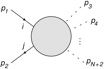
Figure 3: The amplitude for the production of $N$ colour-singlet particles from a quark-antiquark pair, without final state QCD radiation.

One may write the LO amplitude as

$$A\left(\{p_{i}\}\right)\,=\,\delta_{ij}\,\bar{v}(p_{2})\,{\cal A}\left(\{p_{i}\}\right)u(p_{1})\,,$$ (4.1)

where $i$, $j$ are the colour indices of the incoming quark and antiquark, and the factor ${\cal A}(\{p_{i}\})$, matrix-valued in spinor space, is the quantity entering Eq. (2.6), namely the leading-order amplitude with external wave functions removed. Following the procedure adopted in the gluon case, we may decompose the NLO amplitude, before contraction with external spinors, according to

$${\cal A}^{\sigma}_{\rm\,NLP}\,=\,{\cal A}_{\rm\,scal.}^{\sigma}+{\cal A}_{\rm\,spin}^{\sigma}+{\cal A}_{\rm\,orb.}^{\sigma}\,,$$ (4.2)

where the three terms on the right-hand side denote the scalar-like, spin, and orbital angular momentum contributions, and we have suppressed spinor indices (as well as color labels) for brevity. For the scalar and orbital angular momentum contributions, which do not depend explicitly on the spin (apart from replacing the vector indices on the leading-order amplitude with spinor indices), the arguments of the previous section may be repeated, and one may write

$${\cal A}^{\sigma}_{\rm\,scal.}+{\cal A}^{\sigma}_{\rm\,orb.}\,=\,g_{s}\left(\frac{p_{1}^{\sigma}}{p_{1}\cdot k}-\frac{p_{2}^{\sigma}}{p_{2}\cdot k}\right){\cal A}\left(p_{1}+\delta p_{1},p_{2}+\delta p_{2}\right)\,,$$ (4.3)

where the momentum shifts are defined in Eq. (3.13). Including the (anti)quark wave functions and performing color and spin sums, we then find

$$\left|A_{\rm\,NLP}^{\sigma}\right|^{2}_{\rm\,\,scal.\,+\,orb.}\,=\,g_{s}^{2}N_{c}C_{F}\,\frac{2p_{1}\cdot p_{2}}{p_{1}\cdot k\,p_{2}\cdot k}\,{\rm Tr}\left[\not\!{p_{1}}{\cal A}\left(p_{1}+\delta p_{1},p_{2}+\delta p_{2}\right)\not\!{p}_{2}{\cal A}^{\dagger}\left(p_{1}+\delta p_{1},p_{2}+\delta p_{2}\right)\right]$$

$$\hskip 14.22636pt=\,g_{s}^{2}N_{c}C_{F}\,\frac{s^{2}}{p_{1}\cdot k\,p_{2}\cdot k}\,{\rm Tr}\left[\not\!{n_{1}}{\cal A}\left(p_{1}+\delta p_{1},p_{2}+\delta p_{2}\right)\not\!{n}_{2}{\cal A}^{\dagger}\left(p_{1}+\delta p_{1},p_{2}+\delta p_{2}\right)\right]\,,$$ (4.4)

where in the second line we have introduced the dimensionless vectors

$$n_{i}^{\mu}\,=\,\frac{p_{i}^{\mu}}{\sqrt{s}}\,\qquad\quad i=1,2\,.$$ (4.5)

By comparing Eq. (4.4) with its LO counterpart,

$$\left|A(p_{1},p_{2})\right|\,=\,N_{c}\,s\,{\rm Tr}\left[\not\!{n}_{1}{\cal A}(p_{1},p_{2}){\not\!{n}}_{2}{\cal A}^{\dagger}(p_{1},p_{2})\right]\,,$$ (4.6)

and using Eq. (3.17) we may promote the momentum shift in Eq. (4.4) to apply to the entire squared amplitude. This leads to

$$\left|A_{\rm\,NLP}^{\sigma}\right|^{2}_{\rm\,\,scal.\,+\,orb.}\,=\,\frac{g_{s}^{2}C_{F}}{z}\,\frac{s}{p_{1}\cdot k\,p_{2}\cdot k}\,\left|A\left(p_{1}+\delta p_{1},p_{2}+\delta p_{2}\right)\right|^{2}\,.$$ (4.7)

Note the close resemblance of Eq. (4.7) and Eq. (3.14): they differ only by the color factor and a rescaling by a factor of $z$. We must still, however, add to Eq. (4.7) the interference between the spin-dependent part of the NLO amplitude, and the eikonal amplitude. In the gluon case, this turned out to vanish in Feynman gauge, upon summing over all gluon polarisations, which was allowed at NLP accuracy. For an incoming fermion, we find that the spin contribution does not vanish, and indeed it precisely compensates for the $z$ rescaling observed in Eq. (4.7), recovering the universality of the result.

The spin-dependent part of the NLO amplitude is given by the diagrams of Fig. 4, which evaluate to

$$\epsilon_{\sigma}(k)\,\,t^{a}_{ji}\,\bar{v}(p_{2})\,{\cal A}^{\sigma}_{\rm\,spin}\,u(p_{1}) = -\,{\rm i}\,g_{s}\,t^{a}_{ji}\,k_{\beta}\,\epsilon_{\sigma}(k)\,\bar{v}(p_{2})\left[\frac{{\cal A}\,\Sigma^{\beta\sigma}}{p_{1}\cdot k}+\frac{\Sigma^{\beta\sigma}{\cal A}}{p_{2}\cdot k}\right]u(p_{1})$$ (4.8)

$$= -\,g_{s}\,t^{a}_{ji}\,\epsilon_{\sigma}(k)\,\bar{v}(p_{2})\left[\frac{{\cal A}\,\not\!{k}\,\gamma^{\sigma}}{2p_{1}\cdot k}-\frac{\gamma^{\sigma}\not\!{k}\,{\cal A}}{2p_{2}\cdot k}\right]u(p_{1})\,.$$

Figure 4: Diagrams contributing to the spin-dependent part of the NLO cross-section, where $\bullet$ denotes the magnetic moment coupling of the gluon to the spin of the quark.

In the second line of Eq. (4.8), we anticommuted Dirac matrices and used the physical polarisation condition $k^{\sigma}\epsilon_{\sigma}(k)=0$ to write the result in a form which will be more convenient in what follows. Up to NLP accuracy in the squared amplitude, we only need to consider the interference of Eq. (4.8) with the (leading power) scalar part of the NLO amplitude. Furthermore, since we are considering the emission of a single gluon, we can sum over all polarisations, rather than restricting to physical polarisations only. The relevant contribution to the squared matrix element is then

$$\sum_{\rm colours}2\,{\rm Re}\left[A^{\dagger}_{\rm\,scal.}\,A_{\rm\,spin}\right]_{\rm\,NLP}\,=\,-\,\frac{g_{s}^{2}N_{c}\,C_{F}}{p_{1}\cdot k\,p_{2}\cdot k}\,{\rm Tr}\Big{[}\not\!{p}_{2}\Big{(}{\cal A}\not\!{k}\not\!{p}_{2}+\not\!{p}_{1}\not\!{k}{\cal A}\Big{)}\not\!{p}_{1}{\cal A}^{\dagger}\Big{]}\,.$$ (4.9)

To simplify this further, we may expand the emitted gluon momentum in the Sudakov decomposition

$$k^{\sigma}\,=\,\frac{p_{2}\cdot k}{p_{1}\cdot p_{2}}\,p_{1}^{\sigma}+\frac{p_{1}\cdot k}{p_{1}\cdot p_{2}}\,p_{2}^{\sigma}+k_{T}^{\sigma}\,,\qquad k_{T}\cdot p_{1}\,=\,k_{T}\cdot p_{2}\,=\,0\,.$$ (4.10)

We then observe that, to linear order in $k^{\mu}$, the Dirac trace in Eq. (4.10) cannot depend on $k_{T}$. Indeed, one easily finds

$$\sum_{\rm colours}2\,{\rm Re}\left[A^{\dagger}_{\rm\,scal.}\,A_{\rm\,spin}\right]_{\rm\,NLP}\,=\,-\,g_{s}^{2}N_{c}\,C_{F}\,\frac{2p_{1}\cdot p_{2}}{p_{1}\cdot k\,p_{2}\cdot k}\,\frac{k\cdot(p_{1}+p_{2})}{p_{1}\cdot p_{2}}\,\left|{\cal A}(p_{1},p_{2})\right|^{2}\,.$$ (4.11)

By comparing with the squared scalar part of the amplitude

$$\sum_{\rm colours}A^{\dagger}_{\rm\,scal.}\,A_{\rm\,scal.}\,=\,g_{s}^{2}N_{c}\,C_{F}\,\frac{2p_{1}\cdot p_{2}}{p_{1}\cdot k\,p_{2}\cdot k}\left|{\cal A}(p_{1},p_{2})\right|^{2}\,,$$ (4.12)

we see that the spin-dependent contribution to the squared amplitude can be obtained from the part which is leading power in the gluon momentum, simply through rescaling by the factor

$$-\frac{k\cdot(p_{1}+p_{2})}{p_{1}\cdot p_{2}}\,=\,-\,(1-z)\,,$$ (4.13)

where we have used the momentum parametrisation of Eq. (3.21).

Combining Eq. (4.7) with Eq. (4.12), we see that the rescaling factors cancel at NLP in $(1-z)$. Indeed one may write

$$\left|A_{\rm\,NLP}\right|^{2}\,=\,g_{s}^{2}\,C_{F}\frac{s}{p_{1}\cdot k\,p_{2}\cdot k}\Bigg{\{}\frac{\left|A(p_{1}+\delta p_{1},p_{2}+\delta p_{2})\right|^{2}}{z}-\left|A(p_{1},p_{2})\right|^{2}(1-z)\Bigg{\}}\,.$$ (4.14)

Expanding now in powers of $(1-z)$, one gets to first order

$$\left|A_{\rm NLP}\right|^{2} = g_{s}^{2}\,C_{F}\frac{s}{p_{1}\cdot k\,p_{2}\cdot k}\Bigg{\{}\left|A(p_{1}+\delta p_{1},p_{2}+\delta p_{2})\right|^{2}$$ (4.15)

$$+\,\,\Big{(}\left|A(p_{1}+\delta p_{1},p_{2}+\delta p_{2})\right|^{2}-\left|A(p_{1},p_{2})\right|^{2}\Big{)}(1-z)\Bigg{\}}\,,$$

and one observes that the second line is effectively ${\cal O}(1-z)^{2}$. We find then

$$\left|A_{\rm\,NLP}\right|^{2}\,=\,g_{s}^{2}\,C_{F}\,\frac{s}{p_{1}\cdot k\,p_{2}\cdot k}\left|A(p_{1}+\delta p_{1},p_{2}+\delta p_{2})\right|^{2}\,,$$ (4.16)

which is precisely analogous to Eq. (3.14), except for the replacement of the colour factor, which here is associated with the fundamental rather than adjoint representation of the gauge group. Once again, at NLP, Eq. (4.16) can be used in a fully differential implementation for the final state kinematics.

Having obtained Eq. (4.16), one may form the cross-section by integrating with the $(N+1)$-body phase space, exactly as was done in the gluon case. One finds then

$$\frac{d\hat{\sigma}_{\rm\,NLP}^{(qq)}}{dz}\,=\,C_{F}\,K_{\rm NLP}\left(z,\epsilon\right)\hat{\sigma}_{\rm Born}^{(qq)}\left(zs\right)\,,$$ (4.17)

with the same factor $K_{\rm NLP}\left(z,\epsilon\right)$, given in Eq. (3.27).

A first check on this result is that it reproduces the NLO K-factor for Drell-Yan production of a vector boson of invariant mass $Q^{2}$, where one has

$$z\,=\,\frac{Q^{2}}{s}\,.$$ (4.18)

In this case, as for any $2\to 1$ process, the LO partonic cross section has support only on the partonic threshold: for Drell-Yan production,

$$\sigma_{\rm Born}^{(qq)}(s)\,\propto\,\delta(Q^{2}-s)\,=\,\frac{1}{s}\,\delta\left(\frac{Q^{2}}{s}-1\right)\,,$$ (4.19)

so that the LO cross section with shifted kinematics is

$$\sigma_{\rm Born}^{(qq)}(zs)\,\propto\,\delta\left(Q^{2}-zs\right)\,=\,\frac{1}{s}\,\delta\left(\frac{Q^{2}}{s}-z\right)\,.$$ (4.20)

The delta-function imposes the correct definition of the threshold variable at NLO, while the rest of the cross section is unaffected by the shift in kinematics. To compare with standard results, we must note that the $\overline{\rm MS}$ scale $\overline{\mu}^{2}$ is usually set equal to the final state invariant mass $Q^{2}$. To this end, one may write

$$\left(\frac{\mu^{2}}{s}\right)^{\epsilon}\,=\,\left(\frac{\mu^{2}}{Q^{2}}\right)^{\epsilon}\left(\frac{Q^{2}}{s}\right)^{\epsilon}\rightarrow z^{\epsilon}\,,$$ (4.21)

so that Eq. (3.26) becomes

$$\frac{d\hat{\sigma}_{\rm\,NLP}^{qq}}{dz} = \frac{\alpha_{s}}{\pi}\,C_{F}\,z^{\epsilon}\left[\frac{2-2{\cal D}_{0}(z)}{\epsilon}+4{\cal D}_{1}(z)-4\log(1-z)\right]\sigma_{\rm Born}^{(qq)}(zs)$$ (4.22)

$$= \frac{\alpha_{s}}{4\pi}\,C_{F}\,\left[\frac{8-8{\cal D}_{0}(z)}{\epsilon}+16{\cal D}_{1}(z)-16\log(1-z)+8\right]\,\sigma_{\rm Born}^{(qq)}(zs)\,,$$

which precisely agrees with the well-known results quoted for example in Refs. [64, 21].

5 Single Higgs boson production via gluon fusion

Having presented our results for both quark- and gluon-induced colour-singlet particle production, we now examine a first significant application of the gluon result, Eq. (3.27): the single production of Higgs bosons in the gluon fusion channel. As is well known, this is is the principal production mode for Higgs bosons at the LHC, and higher-order QCD corrections have been studied in great detail and with great efforts in recent years. In the effective field theory with the top quark integrated out, they have been calculated up to N³LO in perturbation theory [65, 66, 67, 68, 15, 18, 17, 16, 14]. Top-mass effects are know exactly at NLO [69], and have been studied at NNLO as a power expansion in $m_{h}^{2}/m_{t}^{2}$ [70, 71]. Here we will see how the intricate top mass dependence at NLO simplifies considerably in the threshold region, including NLP corrections.

At leading order, the incoming gluons couple to the Higgs boson via a top-quark loop, as shown in Fig. 5(a).

Figure 5: (a) Leading order diagram for the production of a Higgs boson via gluon fusion; (b) Contact interaction in the large top mass limit; (c) Contact interaction for radiation of an extra gluon.

The leading order cross-section for this process (see for example [65]) can be written as

$$\sigma^{h}_{\rm\,Born}(s)\,=\,\frac{\alpha_{s}^{2}}{\pi}\,\frac{m_{h}^{2}}{576v^{2}}\,(1+\epsilon)\,F(\tau,\epsilon)\,\delta(s-m_{h}^{2})\,,$$ (5.1)

where $m_{h}$ and $v$ are the Higgs mass and vacuum expectation value respectively. The form factor $F(\tau,\epsilon)$ depends on the dimensionless variable

$$\tau\,=\,\frac{s}{4m_{t}^{2}}\,,$$ (5.2)

and it is given by [65]

$$F(\tau,\epsilon)\,=\,\frac{9}{4}\frac{1}{\tau^{2}}\left|1+\left(1-\frac{1}{\tau}\right)\arcsin^{2}\left(\sqrt{\tau}\right)\right|^{2}\,+\,{\cal O}(\epsilon)\,,$$ (5.3)

with a normalisation chosen so that $F(\tau,\epsilon)\to 1$ as $\tau\to 0$. The cross section with kinematics shifted according to Eq. (3.15) can then be written as

$$\sigma^{h}_{\rm Born}(zs)\,=\,\frac{\alpha_{s}^{2}}{\pi}\,\frac{z}{576v^{2}}\,(1+\epsilon)\,F\left(z\tau,\epsilon\right)\delta\left(z-\frac{m_{h}^{2}}{s}\right)\,.$$ (5.4)

Substituting this result into Eq. (3.26) and expanding in powers of $(1-z)$ and $\epsilon$ one finds

$$\frac{d\sigma^{h}_{\rm NLP}}{dz}\,=\,\frac{\alpha_{s}^{3}C_{A}}{288\pi^{2}v^{2}}\,F(z\tau,\epsilon)\left(\frac{2-{\cal D}_{0}(z)}{\epsilon}+2{\cal D}_{1}(z)-{\cal D}_{0}(z)-4\log(1-z)+2\right)\,.$$ (5.5)

It is easy to check that Eq. (5.5) agrees with the known analytic NLO result of Ref. [65] in the $m_{t}\to\infty$ limit. We note, however, that the result of Eq. (5.5) is much more informative: it includes the full dependence on the top quark mass up to NLP order, and can thus be applied for arbitrary $m_{t}$. This is a remarkable simplification of the intricate result of Ref. [69] for the full $m_{t}$ dependence: after shifting the kinematics of the leading order result, the resulting K-factor is entirely independent of the top quark mass, which makes the formula especially simple to apply in practical applications .

It is interesting to examine the anatomy of the result in Eq. (5.5) in slightly more detail. If one were to calculate the NLO cross section by starting manifestly in the large top mass limit (i.e. by using an effective field theory), the leading order graph would contain an effective point-like interaction coupling the two incoming gluons to a Higgs, as shown in Fig. 5(b). At NLO, one can radiate the extra gluon from either of the incoming gluons, and one must also include the additional effective coupling shown in Fig. 5(c), namely a point-like interaction between three gluons and a Higgs boson. If one resolves the top quark loop as in Fig. 5(a), this extra interaction corresponds to emissions from inside the top quark loop. In the NLP calculation, there is no need to include any additional diagrams to capture these contributions: they are generated precisely by the orbital angular momentum contributions in Eq. (3.6): therefore, as the above analysis reveals, we can choose to associate these terms with a shift in the kinematics of the leading order result, up to corrections subleading in soft momentum. Seen from the point of view of the effective field theory at large $m_{t}$, it is highly non-trivial that such a shift captures the contribution of higher-order operators in the effective Lagrangian.

6 Multiple Higgs boson production

In the previous section we have tested our main result, given by Eq. (3.26) for gluon scattering, by reproducing known results in the cross section for single Higgs boson production via gluon fusion. We now consider the case of Higgs boson pair production, a process of ongoing interest at the LHC, due to its potential role in extracting the Higgs boson self-coupling. Analytic results for this process are known up to NNLO in the large top mass limit [46, 47, 48], but only at leading order with full top mass dependence [50, 51]. Further studies have looked at systematically improving the effective field theory results by including leading-power threshold effects [54], or contributions suppressed by powers of the top mass [55]. Recently, numerical results at NLO accuracy with full top mass dependence have become available [52] (see also [53]). This, however, does not preclude the desire for analytic results, which can serve to improve the efficiency of numerical computations, whilst also providing clues regarding higher-order structures in perturbation theory. This is especially true in Higgs boson pair production, given that the large top mass limit is not a good approximation, unlike the case of single Higgs production. The leading order diagrams for Higgs pair production are shown in Fig. 6, and the leading order amplitude may be written as

Figure 6: Leading-order diagrams contributing to Higgs boson pair production.

$${\cal A}_{\mu\nu}\,=\,\frac{\alpha_{s}}{2\pi v^{2}}\Big{[}\left(C_{\triangle}F_{\triangle}+C_{\Box}F_{\Box}\right)\,T_{0,\,\mu\nu}+C_{\Box}G_{\Box}\,T_{2,\,\mu\nu}\Big{]}\,,$$ (6.1)

where (in the Standard Model)

$$C_{\triangle}\,=\,\frac{3m_{h}^{2}}{s-m_{h}^{2}}\,,\qquad C_{\Box}\,=\,1\,,$$ (6.2)

and $F_{\triangle}$, $F_{\Box}$, $G_{\Box}$ are form factors arising from the triangle and box graphs, as indicated by the subscripts. They depend on the Higgs boson and top masses, as well as the partonic centre of mass energy $s$ and the other Mandelstam invariants

$$t = -\frac{1}{2}\left[s-2m_{h}^{2}-s\sqrt{1-\frac{4m_{h}^{2}}{s}}\cos\theta\right]\,,$$

$$u = -\frac{1}{2}\left[s-2m_{h}^{2}+s\sqrt{1-\frac{4m_{h}^{2}}{s}}\cos\theta\right]\,.$$ (6.3)

The basis tensors $T_{s,\,\mu\nu}$, with $s=0,2$, in Eq. (6.1) are associated with the exchange of spin 0 and spin 2 in the $s$ channel, respectively. Denoting the gluon momenta by $p_{1}$ and $p_{2}$ and the Higgs boson momenta by $p_{3}$ and $p_{4}$, their explicit forms are

$$T_{0}^{\mu\nu} = p_{1}\cdot p_{2}\,\eta^{\mu\nu}-p_{1}^{\nu}\,p_{2}^{\mu}\,,$$ (6.4)

$$T_{2}^{\mu\nu} = p_{1}\cdot p_{2}\,\eta_{\mu\nu}+\frac{1}{p_{T}^{2}}\Big{[}m_{h}^{2}\,\,p_{1}^{\nu}\,p_{2}^{\mu}-2p_{2}\cdot p_{3}\,p_{1}^{\nu}\,p_{3}^{\mu}-2p_{1}\cdot p_{3}\,p_{2}^{\mu}\,p_{3}^{\nu}+2p_{1}\cdot p_{2}\,p_{3}^{\mu}\,p_{3}^{\nu}\Big{]}\,,$$

where

$$p_{T}^{2}\,=\,\frac{2(p_{1}\cdot p_{3})(p_{2}\cdot p_{3})}{p_{1}\cdot p_{2}}-m_{h}^{2}\,.$$ (6.5)

With these notations, the leading-order distribution in the Mandelstam invariant $t$ can be written as [46]

$$\frac{d\hat{\sigma}_{\rm Born}^{hh}}{dt}\,=\,\frac{\alpha_{s}^{2}}{8\pi^{3}}\,\frac{1}{512\,v^{4}}\left[\big{|}C_{\triangle}F_{\triangle}+C_{\Box}F_{\Box}\big{|}^{2}+\big{|}C_{\Box}G_{\Box}\big{|}^{2}\right]\,.$$ (6.6)

This expression simplifies considerably in the large top mass limit, where

$$F_{\triangle}\,\to\,\frac{2}{3}\,,\qquad F_{\Box}\,\to\,-\frac{2}{3}\,,\qquad G_{\Box}\,\to\,0\,,$$ (6.7)

so that Eq. (6.6) becomes

$$\frac{d\hat{\sigma}^{hh}_{\rm Born}}{dt}\,=\,\frac{\alpha_{s}^{2}}{16\pi^{3}}\,\frac{1}{576\,v^{4}}\left(\frac{4m_{h}^{2}-s}{s-m_{h}^{2}}\right)^{2}\,.$$ (6.8)

We observe that, in the large top mass limit, the leading-order cross section vanishes at threshold, as $s\to 4m_{h}^{2}$, due to the cancellation between the box and triangle contributions. This property is one of the reasons that make the large top mass limit a poor approximation in Higgs boson pair production, necessitating the calculation of higher order corrections with full $m_{t}$ dependence. It also causes problems when trying to define a K-factor as a function of the variable $z$. Ordinarily, one would divide the NLO cross section by the LO one, however this becomes ill-defined in the threshold region $z\to 1$. In Ref. [46] this problem is circumvented by dividing by the LO cross section with kinematics shifted according to Eq. (3.17). The resulting K-factor thus matches precisely the quantity defined in Eq. (3.26).

With this convention, the NLO cross section for Higgs boson pair production, up to NLP accuracy, can be written as

$$z\,\frac{d\sigma_{\rm NLP}^{hh}}{dz}\,=\,\frac{\alpha_{s}}{3\pi}\,C_{A}\,\left(\frac{\overline{\mu}^{2}}{s}\right)^{\epsilon}\left[\frac{12-6{\cal D}_{0}(z)}{\epsilon}+12{\cal D}_{1}(z)-24\log(1-z)\right]\sigma^{hh}_{\rm Born}\left(zs\right)\,,$$ (6.9)

where we have extracted an explicit factor of $z$ on the left-hand side, to match the conventions adopted in Ref. [46]. In the large top mass limit, Eq. (6.9) reproduces the results of Ref. [46]. As in the case of single Higgs production, however, the result is much more powerful, in that it applies to the full top mass dependence. Eq. (6.9) thus provides an explicit analytic form of the cross section, at NLO in perturbation theory, and up to NLP in the threshold variable $(1-z)$. This extends the results of Ref. [54], which considered supplementing the fixed-order cross section with threshold effects at leading power only. Ref. [55], on the other hand, studied the systematic improvement of the large top mass limit, by including corrections expressed as a power series in $m_{h}^{2}/m_{t}^{2}$. The authors found that the convergence of this expansion could be dramatically improved by factorising the leading order cross-section with exact top mass dependence. The results of this paper explain why this is so: indeed, we find that, to first subleading order in the threshold expansion, the NLO cross section can be completely expressed in terms of the leading-order cross section with shifted kinematics, and with full top mass dependence.

Returning to the large top mass limit, we can go further and consider triple Higgs production, a process for which analytic NLO corrections were presented recently in Ref. [49]. If we denote the invariant mass of the triple Higgs system by $M_{3h}$, and we set the $\overline{\rm MS}$ scale according to $\mu^{2}=M_{3h}^{2}$, the NLO cross section in the gluon fusion channel can be written as [49]

$$M_{3h}^{2}\,\,\frac{d\sigma^{hhh}}{dM_{3h}^{2}}\,=\,\frac{\alpha_{s}}{2\pi}\,\sigma^{hhh}_{\rm Born}\left(zs\right)\,\eta(z)\,,$$ (6.10)

with

$$\eta(z) = 24{\cal D}_{1}(z)-24z\left(-z+z^{2}+2\right)\log(1-z)$$ (6.11)

$$\quad-\,\frac{12(z^{2}+1-z)^{2}}{1-z}\log(z)-11(1-z)^{3}+C^{(\delta)}_{3h}\delta(1-z)\,,$$

where $C^{(\delta)}_{3h}$ can be read off from Ref. [49], and does not affect our arguments. Expanding to NLP in $(1-z)$, we may rewrite Eq. (6.10) as

$$z\,\frac{d\sigma^{hhh}}{dz}\,=\,\frac{\alpha_{s}}{4\pi}\,C_{A}\,\Big{[}16{\cal D}_{1}(z)-32\log(1-z)+8+{\cal O}(1-z)\Big{]}\,\sigma^{hhh}_{\rm Born}\left(zs\right)\,.$$ (6.12)

This result is indeed reproduced from Eq. (3.26): implementing the scale choice as in Eq. (4.21), one can rewrite Eq. (3.26) in the present case as

$$z\,\frac{d\sigma^{hhh}}{dz}\,=\,\frac{\alpha_{s}}{4\pi}\,C_{A}\,\left[\frac{16-8{\cal D}_{0}(z)}{\epsilon}+16{\cal D}_{1}(z)-32\log(1-z)+8\right]\,\sigma^{hhh}_{\rm Born}\left(zs\right)\,;$$ (6.13)

extracting the finite part in the $\overline{\rm MS}$ scheme, one finds precise agreement with Eq. (6.12).

7 Vector boson pair production

In the preceding two sections, we have illustrated the application of our general expression for the NLO K-factor in the gluon channel. In order to verify and illustrate the quark result, Eq. (4.17), in a non-trivial case, it is instructive to see how known matrix elements in vector boson pair production can be reproduced. This calculation is also an important illustration of the fact that our prediction, while based on power counting in the threshold variable $z$, applies to the fully differential squared amplitude, and not only to the integrated cross section. As an example, we consider di-boson production,

$$q(p_{1})+\bar{q}(p_{2})\,\rightarrow\,V(p_{3})+V(p_{4})\,,$$ (7.1)

where $V$ is an electroweak gauge boson. Let us start with di-photon production, the amplitudes for which can be found in Ref. [59] up to NLO, in four spacetime dimensions. The squared LO matrix element for this process, summed and averaged over colours and spins, is given by

$$\overline{\left|A^{\gamma\gamma}_{\rm Born}\right|^{2}}\,=\,\frac{2e_{q}^{4}}{N_{c}}\,\frac{t^{2}+u^{2}}{tu}\,=\,\frac{4e_{q}^{4}}{N_{c}}\,\frac{1+\cos^{2}\theta}{1-\cos^{2}\theta}\,,$$ (7.2)

where $e_{q}$ is the electromagnetic charge of the quark. One may now consider the radiation of an additional gluon, leading to the process

$$q(p_{1})+\bar{q}(p_{2})\,\rightarrow\,V(p_{3})+V(p_{4})+g(k)\,.$$ (7.3)

Computing the di-photon cross section at NLO, one must include squared Born matrix element for the process in Eq. (7.3), again summed and averaged over colours and spins. It is given by [59]

$$\overline{\left|A_{\rm NLO}^{\gamma\gamma g}\right|^{2}}\,=\,\frac{e_{q}^{4}}{N_{c}}\,g_{s}^{2}C_{F}\,\frac{s\,\sum_{i}(p_{1}\cdot k_{i})(p_{2}\cdot k_{i})\left[(p_{1}\cdot k_{i})^{2}+(p_{2}\cdot k_{i})^{2}\right]}{\prod_{i}(p_{1}\cdot k_{i})(p_{2}\cdot k_{i})}\,,\qquad k_{i}\in\{p_{3},p_{4},k\}\,.$$ (7.4)

Our aim is to show that, up to NLP accuracy, this matrix element can be obtained by shifting kinematics in the LO squared amplitude, as dictated by Eq. (4.16). To this end, one may rescale the gluon momentum as $k\to\lambda k$ in Eq. (7.4), and expand to next-to-leading power in $\lambda$, before setting $\lambda\to 1$. Next, one can parametrise the momenta in the centre of mass frame of the $VV$ system, as (see for example Ref. [60])

$$p_{1} = p_{1}^{0}\,(1,0,0,1)\,,\quad p_{2}\,\,=\,\,p_{2}^{0}\,(1,0,\sin\psi,\cos\psi)\,,\quad k\,\,=\,\,k^{0}\,(1,0,\sin\psi^{\prime},\cos\psi^{\prime})$$

$$p_{3} = \frac{\sqrt{s_{2}}}{2}\,\big{(}1,\beta_{z}\sin\theta_{2}\sin\theta_{1},\beta_{z}\cos\theta_{2}\sin\theta_{1},\beta_{z}\cos\theta_{1}\big{)}\,,$$

$$p_{4} = \frac{\sqrt{s_{2}}}{2}\,\big{(}1,-\beta_{z}\sin\theta_{2}\sin\theta_{1},-\beta_{z}\cos\theta_{2}\sin\theta_{1},-\beta_{z}\cos\theta_{1}\big{)}\,,$$ (7.5)

where

$$p_{1}^{0}\,=\,\frac{s+t_{k}}{2\sqrt{s_{2}}}\,,\quad p_{2}^{0}\,=\,\frac{s+u_{k}}{2\sqrt{s_{2}}}\,,\quad k^{0}\,=\,-\frac{t_{k}+u_{k}}{2\sqrt{s_{2}}}\,,$$

$$\cos\psi\,=\,1-\frac{s}{2p_{1}^{0}p_{2}^{0}}\,,\quad\cos\psi^{\prime}\,=\,1+\frac{t_{k}}{2p_{1}^{0}k^{0}}\,,\quad\beta_{z}\,=\,\sqrt{1-\frac{4m_{V}^{2}}{zs}}\,,$$ (7.6)

and we have introduced the invariants

$$t_{k}\,=\,(p_{1}-k)^{2}\,,\qquad u_{k}\,=\,(p_{2}-k)^{2}\,,\qquad s_{2}\,=\,s+t_{k}+u_{k}\,.$$ (7.7)

Note that in these notations the threshold variable is $\xi=1-z=1-s_{2}/s$. With these definitions, we can now expand to first subleading power in the gluon energy, and set $m_{V}=0$ for the di-photon case. The result is

$$\overline{\left|A_{\rm NLP}^{\gamma\gamma g}\right|^{2}}\,=\,g_{s}^{2}C_{F}\,\frac{s}{p_{1}\cdot k\,p_{2}\cdot k}\,\frac{4e_{q}^{4}}{N_{c}}\,\bigg{[}\frac{1+\cos^{2}\theta_{1}}{1-\cos^{2}\theta_{1}}-\frac{8\sin\theta_{1}\cos\theta_{1}\cos\theta_{2}}{\left(1-\cos^{2}\theta_{1}\right)^{2}}\frac{\sqrt{p_{1}\cdot k\,p_{2}\cdot k}}{s}\bigg{]}\,,$$ (7.8)

By performing the same procedure, one may easily show that the LO amplitude of Eq. (7.2), evaluated with the kinematic shifts defined in Eq. (3.13), yields

$$\overline{\left|A_{\rm Born}^{\gamma\gamma}\left(p_{1}+\delta p_{1},p_{2}+\delta p_{2}\right)\right|^{2}}\,=\,\frac{4e_{q}^{4}}{N_{c}}\,\bigg{[}\frac{1+\cos^{2}\theta_{1}}{1-\cos^{2}\theta_{1}}-\frac{8\sin\theta_{1}\cos\theta_{1}\cos\theta_{2}}{(1-\cos^{2}\theta_{1})^{2}}\frac{\sqrt{p_{1}\cdot k\,p_{2}\cdot k}}{s}\bigg{]}\,.$$ (7.9)

We therefore see that Eq. (7.8) explicitly confirms the expectations raised by Eq. (4.16).

A similar exercise may be carried out for $W^{+}W^{-}$ production: the NLO squared amplitudes for this process (again in four spacetime dimensions) may be found in Ref. [60]. The Born-level squared matrix element, summed and averaged over colours and spins, is given by

$$\overline{\left|A_{\rm Born}^{WW}\right|^{2}}\,=\,\frac{1}{4N_{c}}\left[c^{tt}_{i}\,F_{i}^{(0)}(s,t)-c^{ts}_{i}(s)\,J_{i}^{(0)}(s,t)+c^{ss}_{i}(s)\,K_{i}^{(0)}(s,t)\right]\,,$$ (7.10)

where $c^{tt}_{i}$, $c^{ss}_{i}$ and $c^{ts}_{i}$ are coefficients associated with $t$-channel, $s$-channel and interference graphs, respectively, for a quark of flavour $i$, and can be found in Ref. [60]. The remaining functions of Mandelstam invariants are given by

$$F_{i}^{(0)}(s,t) = 16\left(\frac{ut}{m_{W}^{4}}-1\right)\left(\frac{1}{4}+\frac{m_{W}^{4}}{t^{2}}\right)+16\,\frac{s}{m_{W}^{2}}\,,$$

$$J_{i}^{(0)}(s,t) = 16\left(\frac{ut}{m_{W}^{4}}-1\right)\left(\frac{s}{4}-\frac{m_{W}^{2}}{2}-\frac{m_{W}^{4}}{t}\right)+16s\left(\frac{s}{m_{W}^{2}}-2+2\,\frac{m_{W}^{2}}{t}\right)\,,$$

$$K^{(0)}_{i}(s,t) = 8\left(\frac{ut}{m_{W}^{4}}-1\right)\left(\frac{s^{2}}{4}-sm_{W}^{2}+3m_{W}^{4}\right)+8s^{2}\left(\frac{s}{m_{W}^{2}}-4\right)\,.$$ (7.11)

Similarly, the NLO squared matrix element including the radiation of a gluon, for the $q\bar{q}$ initial state, also summed and averaged over colours and spins, is given by

$$\overline{\left|A_{\rm NLO}^{WWg}\right|^{2}}\,=\,\frac{4\pi\alpha_{s}C_{F}}{N_{c}}\,\frac{s}{t_{k}u_{k}}\,\Big{[}c_{i}^{tt}\,\widehat{X}_{i}-c_{i}^{ts}(zs)\,\widehat{Y}_{i}+c_{i}^{ss}(zs)\,\widehat{Z}_{i}\Big{]}\,,$$ (7.12)

where the functions $\widehat{X}_{i}$, $\widehat{Y}_{i}$ and $\widehat{Z}_{i}$ have been obtained by rescaling the corresponding functions $X_{i}$, $Y_{i}$ and $Z_{i}$, given in Appendix D of Ref. [60], extracting the singular prefactor $-4s/(t_{k}u_{k})$. Parametrising momenta as in Eq. (7.5), one may expand each function up to NLP in $\xi=(1-z)$, using the same procedure as outlined above for the di-photon matrix element. Introducing the notation $\rho=m_{W}^{2}/s$, the results can be written as

$$\widehat{X}_{i}\Big{|}_{\rm NLP} = \frac{32}{(4\rho-1)\big{[}1-2\rho+(4\rho-1)\cos\theta_{1}\big{]}^{3}}\,\bigg{\{}\cos^{2}\theta_{1}\left(32\rho^{3}-32\rho^{2}+10\rho-1\right)$$

$$+\,\cos\theta_{1}\left(96\rho^{4}-112\rho^{3}+70\rho^{2}-20\rho+2\right)-16\rho^{4}+44\rho^{3}-34\rho^{2}$$

$$+10\rho-1+\xi\,\Big{[}\cos^{2}\theta_{1}\left(128\rho^{4}-96\rho^{3}+24\rho^{2}-2\rho\right)+\cos\theta_{1}\left(32\rho^{3}\right.$$

$$\left.-16\rho^{2}+2\rho\right)+16\rho^{3}-4\rho^{2}\Big{]}\bigg{\}}\,-\,\frac{\cos^{2}\theta_{1}}{(4\rho-1)}\bigg{[}192\rho-112+\frac{20}{\rho}-\frac{1}{\rho^{2}}$$

$$+\,\xi\,\left(128\rho-96+\frac{24}{\rho}-\frac{2}{\rho^{2}}\right)\bigg{]}+\frac{1}{\rho^{2}}+\frac{12}{\rho}-16+\,\xi\,\left(\frac{2}{\rho^{2}}+\frac{12}{\rho}\right)$$

$$+\frac{\sin\psi\cos\theta_{2}\sin\theta_{1}}{\big{[}1-2\rho+(4\rho-1)\cos\theta_{1}\big{]}^{3}}\,\Bigg{[}\cos^{4}\theta_{1}\,\bigg{(}1024\rho^{3}-1280\rho^{2}+640\rho-160$$

$$+\frac{20}{\rho}-\frac{1}{\rho^{2}}\bigg{)}+\cos^{3}\theta_{1}\left(-1536\rho^{3}+2304\rho^{2}-1344\rho+384-\frac{54}{\rho}+\frac{3}{\rho^{2}}\right)$$

$$+\cos^{2}\theta_{1}\left(768\rho^{3}-1344\rho^{2}+912\rho-300+\frac{48}{\rho}-\frac{3}{\rho^{2}}\right)$$

$$+\cos\theta_{1}\left(-640\rho^{3}+768\rho^{2}-360\rho+92-\frac{14}{\rho}+\frac{1}{\rho^{2}}\right)-256\rho^{2}+128\rho-16\Bigg{]}\,,$$

$$\widehat{Y}_{i}\Big{|}_{\rm NLP} = \frac{32s\rho}{\big{[}1-2\rho+(4\rho-1)\cos\theta_{1}\big{]}^{2}}\bigg{[}\cos\theta_{1}(\rho+2)+2\rho^{2}+3\rho-2$$ (7.14)

$$+\,\xi\rho\,\Big{(}\cos\theta_{1}(4\rho-1)+5\Big{)}\bigg{]}+s\,\bigg{\{}\cos^{2}\theta_{1}\left(96\rho-80+\frac{18}{\rho}-\frac{1}{\rho^{2}}\right)$$

$$+\,8\cos\theta_{1}\left(-8\rho+1\right)-16\rho-16+\frac{10}{\rho}+\frac{1}{\rho^{2}}+\xi\,\bigg{[}\cos^{2}\theta_{1}\left(64\rho-80+\frac{28}{\rho}-\frac{3}{\rho^{2}}\right)$$

$$+8\cos\theta_{1}\left(-4\rho+1\right)-16+\frac{20}{\rho}+\frac{3}{\rho^{2}}\bigg{]}\bigg{\}}$$

$$+\,\frac{s\sin\psi\cos\theta_{2}\sin\theta_{1}}{\big{[}\left(4\rho-1\right)\cos\theta_{1}+1-2\rho\big{]}^{2}}\,\Bigg{[}\cos^{3}\theta_{1}\left(-512\rho^{3}+768\rho^{2}-448\rho+128-\frac{18}{\rho}+\frac{1}{\rho^{2}}\right)$$

$$+\,\cos^{2}\theta_{1}\left(768\rho^{3}-1088\rho^{2}+656\rho-204+\frac{32}{\rho}-\frac{2}{\rho^{2}}\right)$$

$$+\,\cos\theta_{1}\,\left(-384\rho^{3}+512\rho^{2}-280\rho+84-\frac{14}{\rho}+\frac{1}{\rho^{2}}\right)-192\rho^{2}+64\rho-4\Bigg{]}\,,$$

$$\widehat{Z}_{i}\Big{|}_{\rm NLP} = s^{2}\,\Bigg{\{}\cos^{2}\theta_{1}\left(-288\rho^{2}+192\rho-62+\frac{10}{\rho}-\frac{1}{2\rho^{2}}\right)-24\rho-18+\frac{4}{\rho}+\frac{1}{2\rho^{2}}$$ (7.15)

$$+\,\xi\,\bigg{[}\cos^{2}\theta_{1}\left(-192\rho^{2}+192\rho-92+\frac{22}{\rho}-\frac{2}{\rho^{2}}\right)-24\rho-36+\frac{12}{\rho}+\frac{2}{\rho^{2}}\bigg{]}\Bigg{\}}$$

$$+\,s^{2}\,\sin\psi\cos\theta_{2}\sin\theta_{1}\cos\theta_{1}\left(96\rho^{2}-80\rho+30-\frac{6}{\rho}+\frac{1}{2\rho^{2}}\right)\,.$$

We have explicitly checked that the same results are obtained from Eq. (4.16), where for the right-hand side one must use the LO squared amplitude given in Eq. (7.10), with momenta shifted according to Eq. (3.13). This is a highly non-trivial cross-check: comparing Eqs. (7 - 7.15) with the di-photon case given in Eq. (7.8), one sees that the $WW$ case involves a much more complicated dependence on the opening angle $\theta_{1}$, and the partonic centre of mass energy $s$. A similar analysis could be carried out for $ZZ$ production [72], and also to provide analytic information for triple vector boson production, numerical results for which have been presented in refs. [73, 74].

8 Conclusion

In this paper, we have considered the hadro-production of an arbitrary heavy colourless system, in both the gluon-fusion and quark-antiquark-annihilation channels, near partonic threshold for the production of the selected final state. Our starting point is an all-order factorisation formula for the relevant scattering amplitudes, introduced in Refs. [23, 24], given here in Eq. (2), and valid to next-to-leading power in the threshold expansion. Specialising this formula to NLO in the strong coupling, we have observed how the general expression simplifies, and takes the form of a next-to-soft theorem, as derived for example in [43, 44, 45]. This simple expression, in turn, leads to a universal form for the transition probability, completely differential in the final state variables, and proportional to the Born-level transition probability, computed with a specific shift for the initial parton momenta. The result is the same for quarks and gluons (up to a trivial substitution of color factors), and is reported in Eqs. (3.14, 4.16). When the transition probability is integrated over final state variables, one finds that the inclusive cross section for the selected process can also be written in a simple and universal factorised form, given here in Eqs. (3.26, 4.17). More precisely, at NLO, and up to next-to-leading power in the threshold expansion, the cross-sections can be written as a universal $K$-factor, multiplying the leading order cross-section with a shifted partonic centre-of-mass energy. All these results apply regardless of whether the leading order process is tree-level or loop-induced, and the resulting K-factors are independent of hard scales such as heavy quark masses.

We have checked our results by reproducing known expressions for the production of up to three Higgs bosons at NLO, in the large top mass limit. Away from this limit, our formula provides new analytic information in the case of Higgs pair production at NLO, where only numerical results are presently known. Furthermore, we explain the observation, made previously in Ref. [55], that the convergence of the large top mass expansion can be improved in this process by factoring out the LO cross-section with exact top mass dependence. In the quark channel, we have shown how our formula is consistent with previous results for the production of photon and $W$ boson pairs, again at the level of differential distributions.

The results we have presented show that, to NLP accuracy, differential and inclusive NLO cross sections for colour-singlet final states are dramatically simpler than exact results, and we expect that they will be very easy to implement in numerical codes, providing checks of existing calculations, and improved approximations for differential distributions when complete results are not available, as is the case for loop induced processes with multi-particle electroweak final states. A detailed phenomenological analysis, including a study of the accuracy of the NLP approximation in different processes and kinematic domains, has been left to future work.

We emphasise that the simple universal expressions that we find at NLO can be systematically improved upon by relying on Eq. (2): in particular, a NLO calculation of the radiative soft function and of the radiative jet functions for quarks and gluons, which is under way, will lead to NLP approximations for cross sections of the type studied in this paper at NNLO level, exploring uncharted territory, in particular for processes which are loop induced and have so far been studied predominantly in the context of effective field theory approximations. We also note that the universal expressions we have derived for inclusive cross sections are also applicable to colourless final states arising beyond the Standard Model, in which case our results can provide a controlled approximation to estimate the size of higher-order corrections in selected models without the need to perform calculations that would be expensive for loop-induced processes.

References

- [1] J. R. Andersen et al., “Les Houches 2015: Physics at TeV Colliders Standard Model Working Group Report,” in 9th Les Houches Workshop on Physics at TeV Colliders (PhysTeV 2015) Les Houches, France, June 1-19, 2015. 2016. 1605.04692.
- [2] G. Sterman, “Summation of large corrections to short distance hadronic cross-sections,” Nucl. Phys. B281 (1987) 310.
- [3] S. Catani and L. Trentadue, “Resummation of the QCD Perturbative Series for Hard Processes,” Nucl. Phys. B327 (1989) 323.
- [4] G. P. Korchemsky and G. Marchesini, “Resummation of large infrared corrections using Wilson loops,” Phys. Lett. B313 (1993) 433–440.
- [5] G. P. Korchemsky and G. Marchesini, “Structure function for large x and renormalization of wilson loop,” Nucl. Phys. B406 (1993) 225–258, hep-ph/9210281.
- [6] H. Contopanagos, E. Laenen, and G. Sterman, “Sudakov factorization and resummation,” Nucl. Phys. B484 (1997) 303–330, hep-ph/9604313.
- [7] S. Forte and G. Ridolfi, “Renormalization group approach to soft gluon resummation,” Nucl. Phys. B650 (2003) 229–270, hep-ph/0209154.
- [8] T. O. Eynck, E. Laenen, and L. Magnea, “Exponentiation of the Drell-Yan cross section near partonic threshold in the DIS and MS-bar schemes,” JHEP 06 (2003) 057, hep-ph/0305179.
- [9] A. Banfi, G. P. Salam, and G. Zanderighi, “Principles of general final-state resummation and automated implementation,” JHEP 03 (2005) 073, hep-ph/0407286.
- [10] T. Becher and M. Neubert, “Threshold resummation in momentum space from effective field theory,” Phys. Rev. Lett. 97 (2006) 082001, hep-ph/0605050.
- [11] G. Luisoni and S. Marzani, “QCD resummation for hadronic final states,” J. Phys. G42 (2015), no. 10, 103101, 1505.04084.
- [12] N. Kidonakis, “Soft-gluon resummations and NNNLO expansions,” PoS EPS-HEP2013 (2013) 432, 1309.1442.
- [13] M. Kramer, E. Laenen, and M. Spira, “Soft gluon radiation in Higgs boson production at the LHC,” Nucl. Phys. B511 (1998) 523–549, hep-ph/9611272.
- [14] C. Anastasiou, C. Duhr, F. Dulat, and B. Mistlberger, “Soft triple-real radiation for Higgs production at N3LO,” JHEP 07 (2013) 003, 1302.4379.
- [15] C. Anastasiou, C. Duhr, F. Dulat, F. Herzog, and B. Mistlberger, “Real-virtual contributions to the inclusive Higgs cross-section at ,” JHEP 1312 (2013) 088, 1311.1425.
- [16] C. Anastasiou, C. Duhr, F. Dulat, E. Furlan, T. Gehrmann, F. Herzog, and B. Mistlberger, “Higgs boson gluon–fusion production at threshold in N3LO QCD,” Phys. Lett. B737 (2014) 325–328, 1403.4616.
- [17] C. Anastasiou, C. Duhr, F. Dulat, E. Furlan, T. Gehrmann, F. Herzog, and B. Mistlberger, “Higgs boson gluon-fusion production beyond threshold in N3LO QCD,” JHEP 03 (2015) 091, 1411.3584.
- [18] C. Anastasiou, C. Duhr, F. Dulat, F. Herzog, and B. Mistlberger, “Higgs Boson Gluon-Fusion Production in QCD at Three Loops,” Phys. Rev. Lett. 114 (2015) 212001, 1503.06056.
- [19] E. Laenen, L. Magnea, and G. Stavenga, “On next-to-eikonal corrections to threshold resummation for the Drell-Yan and DIS cross sections,” Phys. Lett. B669 (2008) 173–179, 0807.4412.
- [20] E. Laenen, G. Stavenga, and C. D. White, “Path integral approach to eikonal and next-to-eikonal exponentiation,” JHEP 0903 (2009) 054, 0811.2067.
- [21] E. Laenen, L. Magnea, G. Stavenga, and C. D. White, “Next-to-eikonal corrections to soft gluon radiation: a diagrammatic approach,” JHEP 1101 (2011) 141, 1010.1860.
- [22] D. Bonocore, E. Laenen, L. Magnea, L. Vernazza, and C. D. White, “The method of regions and next-to-soft corrections in Drell-Yan production,” Phys.Lett. B742 (2015) 375–382, 1410.6406.
- [23] D. Bonocore, E. Laenen, L. Magnea, S. Melville, L. Vernazza, and C. D. White, “A factorization approach to next-to-leading-power threshold logarithms,” JHEP 06 (2015) 008, 1503.05156.
- [24] D. Bonocore, E. Laenen, L. Magnea, L. Vernazza, and C. D. White, “Non-abelian factorisation for next-to-leading-power threshold logarithms,” JHEP 12 (2016) 121, 1610.06842.
- [25] S. Moch and A. Vogt, “Threshold Resummation of the Structure Function F(L),” JHEP 0904 (2009) 081, 0902.2342.
- [26] S. Moch and A. Vogt, “On non-singlet physical evolution kernels and large-x coefficient functions in perturbative QCD,” JHEP 0911 (2009) 099, 0909.2124.
- [27] G. Soar, S. Moch, J. Vermaseren, and A. Vogt, “On Higgs-exchange DIS, physical evolution kernels and fourth-order splitting functions at large x,” Nucl.Phys. B832 (2010) 152–227, 0912.0369.
- [28] A. Almasy, G. Soar, and A. Vogt, “Generalized double-logarithmic large-x resummation in inclusive deep-inelastic scattering,” JHEP 1103 (2011) 030, 1012.3352.
- [29] N. Lo Presti, A. Almasy, and A. Vogt, “Leading large-x logarithms of the quark & gluon contributions to inclusive Higgs-boson and lepton-pair production,” Phys.Lett. B737 (2014) 120–123, 1407.1553.
- [30] D. de Florian, J. Mazzitelli, S. Moch, and A. Vogt, “Approximate N3LO Higgs-boson production cross section using physical-kernel constraints,” 1408.6277.
- [31] G. Grunberg and V. Ravindran, “On threshold resummation beyond leading 1-x order,” JHEP 0910 (2009) 055, 0902.2702.
- [32] G. Grunberg, “Large-x structure of physical evolution kernels in Deep Inelastic Scattering,” Phys.Lett. B687 (2010) 405–409, 0911.4471.
- [33] A. J. Larkoski, D. Neill, and I. W. Stewart, “Soft Theorems from Effective Field Theory,” JHEP 06 (2015) 077, 1412.3108.
- [34] D. W. Kolodrubetz, I. Moult, and I. W. Stewart, “Building Blocks for Subleading Helicity Operators,” JHEP 05 (2016) 139, 1601.02607.
- [35] I. Moult, L. Rothen, I. W. Stewart, F. J. Tackmann, and H. X. Zhu, “Subleading Power Corrections for N-Jettiness Subtractions,” 1612.00450.
- [36] I. Moult, I. W. Stewart, and G. Vita, “A Subleading Operator Basis and Matching for ,” 1703.03408.
- [37] I. Feige, D. W. Kolodrubetz, I. Moult, and I. W. Stewart, “A Complete Basis of Helicity Operators for Subleading Factorization,” 1703.03411.
- [38] H. Gervais, “Soft Photon Theorem for High Energy Amplitudes in Yukawa and Scalar Theories,” 1704.00806.
- [39] H. Gervais, “Soft Graviton Emission at High and Low Energies in Yukawa and Scalar Theories,” 1706.03453.
- [40] F. E. Low, “Bremsstrahlung of very low-energy quanta in elementary particle collisions,” Phys. Rev. 110 (1958) 974–977.
- [41] T. H. Burnett and N. M. Kroll, “Extension of the low soft photon theorem,” Phys. Rev. Lett. 20 (1968) 86.
- [42] V. Del Duca, “High-energy bremsstrahlung theorems for soft photons,” Nucl. Phys. B345 (1990) 369–388.
- [43] E. Casali, “Soft sub-leading divergences in Yang-Mills amplitudes,” JHEP 08 (2014) 077, 1404.5551.
- [44] C. D. White, “Factorization Properties of Soft Graviton Amplitudes,” JHEP 1105 (2011) 060, 1103.2981.
- [45] F. Cachazo and A. Strominger, “Evidence for a New Soft Graviton Theorem,” 1404.4091.
- [46] S. Dawson, S. Dittmaier, and M. Spira, “Neutral Higgs boson pair production at hadron colliders: QCD corrections,” Phys. Rev. D58 (1998) 115012, hep-ph/9805244.
- [47] D. de Florian and J. Mazzitelli, “Higgs Boson Pair Production at Next-to-Next-to-Leading Order in QCD,” Phys. Rev. Lett. 111 (2013) 201801, 1309.6594.
- [48] D. de Florian, M. Grazzini, C. Hanga, S. Kallweit, J. M. Lindert, P. Maierhöfer, J. Mazzitelli, and D. Rathlev, “Differential Higgs Boson Pair Production at Next-to-Next-to-Leading Order in QCD,” JHEP 09 (2016) 151, 1606.09519.
- [49] D. de Florian and J. Mazzitelli, “Two-loop corrections to the triple Higgs boson production cross section,” JHEP 02 (2017) 107, 1610.05012.
- [50] E. W. N. Glover and J. J. van der Bij, “HIGGS BOSON PAIR PRODUCTION VIA GLUON FUSION,” Nucl. Phys. B309 (1988) 282–294.
- [51] T. Plehn, M. Spira, and P. M. Zerwas, “Pair production of neutral Higgs particles in gluon-gluon collisions,” Nucl. Phys. B479 (1996) 46–64, hep-ph/9603205. [Erratum: Nucl. Phys.B531,655(1998)].
- [52] S. Borowka, N. Greiner, G. Heinrich, S. P. Jones, M. Kerner, J. Schlenk, and T. Zirke, “Full top quark mass dependence in Higgs boson pair production at NLO,” JHEP 10 (2016) 107, 1608.04798.
- [53] R. Frederix, S. Frixione, V. Hirschi, F. Maltoni, O. Mattelaer, P. Torrielli, E. Vryonidou, and M. Zaro, “Higgs pair production at the LHC with NLO and parton-shower effects,” Phys. Lett. B732 (2014) 142–149, 1401.7340.
- [54] D. Y. Shao, C. S. Li, H. T. Li, and J. Wang, “Threshold resummation effects in Higgs boson pair production at the LHC,” JHEP 07 (2013) 169, 1301.1245.
- [55] J. Grigo, J. Hoff, K. Melnikov, and M. Steinhauser, “On the Higgs boson pair production at the LHC,” Nucl. Phys. B875 (2013) 1–17, 1305.7340.
- [56] T. Plehn and M. Rauch, “The quartic higgs coupling at hadron colliders,” Phys. Rev. D72 (2005) 053008, hep-ph/0507321.
- [57] F. Maltoni, E. Vryonidou, and M. Zaro, “Top-quark mass effects in double and triple Higgs production in gluon-gluon fusion at NLO,” JHEP 11 (2014) 079, 1408.6542.
- [58] B. Hespel, F. Maltoni, and E. Vryonidou, “Higgs and Z boson associated production via gluon fusion in the SM and the 2HDM,” JHEP 06 (2015) 065, 1503.01656.
- [59] R. Gastmans and T. T. Wu, “The ubiquitous photon: Helicity method for qed and qcd,”. Oxford, UK: Clarendon (1990) 648 p. (International series of monographs on physics, 80).
- [60] S. Frixione, “A next-to-leading order calculation of the cross-section for the production of w+ w- pairs in hadronic collisions,” Nucl. Phys. B410 (1993) 280–324.
- [61] L. J. Dixon, L. Magnea, and G. F. Sterman, “Universal structure of subleading infrared poles in gauge theory amplitudes,” JHEP 0808 (2008) 022, 0805.3515.
- [62] J. Grammer, G. and D. Yennie, “Improved treatment for the infrared divergence problem in quantum electrodynamics,” Phys.Rev. D8 (1973) 4332–4344.
- [63] C. White, “Diagrammatic insights into next-to-soft corrections,” Phys.Lett. B737 (2014) 216–222, 1406.7184.
- [64] R. Hamberg, W. L. van Neerven, and T. Matsuura, “A Complete calculation of the order correction to the Drell-Yan K factor,” Nucl. Phys. B359 (1991) 343–405.
- [65] S. Dawson, “Radiative corrections to higgs boson production,” Nucl. Phys. B359 (1991) 283–300.
- [66] C. Anastasiou and K. Melnikov, “Higgs boson production at hadron colliders in nnlo qcd,” Nucl. Phys. B646 (2002) 220–256, hep-ph/0207004.
- [67] R. V. Harlander and W. B. Kilgore, “Next-to-next-to-leading order higgs production at hadron colliders,” Phys. Rev. Lett. 88 (2002) 201801, hep-ph/0201206.
- [68] V. Ravindran, J. Smith, and W. L. van Neerven, “Nnlo corrections to the total cross section for higgs boson production in hadron hadron collisions,” Nucl. Phys. B665 (2003) 325–366, hep-ph/0302135.
- [69] M. Spira, A. Djouadi, D. Graudenz, and P. M. Zerwas, “Higgs boson production at the LHC,” Nucl. Phys. B453 (1995) 17–82, hep-ph/9504378.
- [70] R. V. Harlander and K. J. Ozeren, “Finite top mass effects for hadronic Higgs production at next-to-next-to-leading order,” JHEP 11 (2009) 088, 0909.3420.
- [71] A. Pak, M. Rogal, and M. Steinhauser, “Finite top quark mass effects in NNLO Higgs boson production at LHC,” JHEP 02 (2010) 025, 0911.4662.
- [72] B. Mele, P. Nason, and G. Ridolfi, “QCD radiative corrections to Z boson pair production in hadronic collisions,” Nucl. Phys. B357 (1991) 409–438.
- [73] A. Lazopoulos, K. Melnikov, and F. Petriello, “QCD corrections to tri-boson production,” Phys. Rev. D76 (2007) 014001, hep-ph/0703273.
- [74] F. Campanario, V. Hankele, C. Oleari, S. Prestel, and D. Zeppenfeld, “QCD corrections to charged triple vector boson production with leptonic decay,” Phys. Rev. D78 (2008) 094012, 0809.0790.