Two-dimensional pulse dynamics and the formation of bound states on electrified falling films

Abstract

The flow of an electrified liquid film down an inclined plane wall is investigated with the focus on coherent structures in the form of travelling waves on the film surface, in particular, single-hump solitary pulses and their interactions. The flow structures are analysed first using a long-wave model, which is valid in the presence of weak inertia, and second using the Stokes equations. For obtuse angles, gravity is destablising and solitary pulses exist even in the absence of an electric field. For acute angles, spatially non-uniform solutions exist only beyond a critical value of the electric field strength; moreover, solitary-pulse solutions are present only at sufficiently high supercritical electric field strengths. The electric field increases the amplitude of the pulses, can generate recirculation zones in the humps, and alters the far-field decay of the pulse tails from exponential to algebraic with a significant impact on pulse interactions. A weak-interaction theory predicts an infinite sequence of bound-state solutions for non-electrified flow, and a finite set for electrified flow. The existence of single-hump pulse solutions and two-pulse bound states is confirmed for the Stokes equations via boundary-element computations. In addition, the electric field is shown to trigger a switch from absolute instability to convective instability, thereby regularising the dynamics, and this is confirmed by time-dependent simulations of the long-wave model.

1 Introduction

Flowing liquid films are central to a wide variety of industrial applications and engineering systems. Spatial heterogeneity in the film thickness, which arises as a natural feature of the dynamics, may be exploited to enhance the intended purpose of the film, for example in promoting heat transfer (e.g. Park & Nosoko, 2003).

Electric fields have been proposed as a viable control mechanism in liquid film flows. Examples include the creation of microscale surface patterning in the absence of inertia and shear (Schäffer et al., 2000), and their suggested use in cylindrical space radiators (Kim et al., 1994). In this study, we discuss the use of an electric field as a means of controlling the dynamics, most notably the formation of solitary and bound-state pulses, in the flow of a liquid film down an inclined plate. A flat film is known to become unstable to long-wave perturbations when the Reynolds number exceeds a critical value that depends on the angle of inclination (Benjamin, 1957; Yih, 1963); for a vertical plate or one inclined at an obtuse angle to the horizontal, the film is unstable at any Reynolds number. For an acute angle of inclination, the flow can be destabilised even at zero Reynolds number by increasing the intensity of the electric field. The surface profile of an unstable film exhibits a rich variety of spatial and temporal structures, ranging from almost harmonic waves at the flow inlet to highly nonlinear wave patterns sufficiently far downstream. Recent reviews of falling film dynamics can be found in Craster & Matar (2009), Kalliadasis et al. (2011) and Ruyer-Quil et al. (2014).

There are numerous theoretical studies of film flow, but those of particular relevance to the present work and which incorporate the effect of a normal electric field include Gonzales & Castellanos (1996), and Tseluiko & Papageorgiou (2006). Here, the full governing equations were simplified using a long-wave asymptotic analysis to derive a fully nonlinear Benney-type equation for the scaled interface location (Benney, 1966), which includes a non-local term encapsulating the effect of the electric field. Tseluiko & Papageorgiou (2006) obtained an even simpler, weakly-nonlinear equation of Kuramoto–Sivashinsky (KS) type with a non-local electric field term. Tseluiko & Papageorgiou (2006) carried out an extensive numerical investigation of the electrified KS equation and found complex dynamical behaviour. Kawahara (1983) (for the non-electrified case) and Tseluiko & Papageorgiou (2010) (for the electrified case) found the inclusion of dispersion to have a regularising effect; in particular solutions evolve into weakly interacting pulses. The regularising effect of dispersion for the non-electrified gKS equation was analysed in detailed by Chang et al. (1995) and Tseluiko et al. (2010). Recently Wray et al. (2017) have derived a fully nonlinear model for an electrified falling film which is valid at finite Reynolds number using a weighted residuals approach. We note that most previous studies have focused on acute inclination angles. Studies of the obtuse inclination angle case are limited in number, but include the recent work by Rohlfs et al. (2017), who adopted a weighted-residuals approach, as well using direct solutions of the Navier–Stokes equations, to study pulses on an inverted film in the absence of an electric field.

Many experiments have been designed to elucidate the behaviour of falling films, quite a number of which have focused on the effects of imposing forced perturbations of a specified frequency at the inlet (e.g. Liu & Gollub, 1994; Nosoko & Miyara, 2004). Solitary waves and saturated almost periodic waves appear close to the inlet at low and high frequencies respectively. Further downstream, the flow is dominated by two-dimensional solitary-wave pulses and their mutual interactions (Liu & Gollub, 1994; Vlachogiannis & Bontozoglou, 2001). After a stage of weak interaction with each other, the two-dimensional solitary pulses experience a secondary instability and develop into three-dimensional localised structures, the highly non-trivial interaction of which eventually gives rise to interfacial turbulence (Demekhin et al., 2010).

It is clear, then, that a study of solitary pulses must lie at the heart of any endeavour to understand the dynamics of a falling film. In this work, we focus on two-dimensional pulses and, in particular, we offer a synthesis of long-wave model calculations and predictions based on fully nonlinear solutions of the Stokes equations. We consider unstable films for both acute and obtuse plate inclination angles, in each case examining steady (in a travelling frame of reference) solitary pulse solutions and bound-state solutions. Such solutions are themselves inherently unstable: the absolute/convective nature of this is examined using an adaptation of the classical Huerre–Monkewitz approach. Finally, we carry out numerical time-dependent simulations and demonstrate for the first time that an absolutely unstable flow can be regularised by increasing the intensity of the electric field, revealing a train of isolated pulses propagating along the film surface.

Although our study is restricted to two-dimensional dynamics, it is important to recognise the potentiality for transverse instabilities. Recently Tomlin et al. (2017) studied the spatiotemporal dynamics of electrified falling films using a multidimensional non-local Kuramoto–Sivashinsky model equation. They found that purely transverse modes for a flat film can become unstable for obtuse inclination angles or when the electric Weber number exceeds a certain threshold value. Despite this finding, two-dimensional studies are nevertheless of importance since two-dimensional states are visited during three-dimensional time evolution (e.g. Kalliadasis et al., 2011) or may act as a preferred state in a controlled system (e.g. Gomes et al., 2017). We also note that the transverse instability of fully-nonlinear electrified two-dimensional travelling-waves has yet to be assessed.

The layout of the paper is as follows. The problem formulation is introduced in § 2. In § 3 we introduce the non-local long-wave model. We use numerical continuation techniques to explore travelling waves, analyse the far-field decay of the long-wave pulses and develop a weak interaction theory for multiple pulses. In § 4 we present fully nonlinear pulse solutions computed using the boundary-element method, including single-hump pulses and two-pulse bound states. In § 5 we discuss the instability of a single-pulse solution and examine its absolute or convective nature. Finally, conclusions and discussion of our results are offered in § 7.

2 Problem formulation

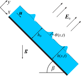
Figure 1: (Color online) Schematic representation of a viscous liquid film flow down an inclined plane wall. Throughout the study, the waves travel in the positive $x$-direction.

We consider a viscous liquid film that flows down a plane wall inclined at angle $\beta$ to the horizontal. The film is exposed to an electric field which acts in the direction normal to the wall and which is uniform with strength $E_{0}$ at infinity, as is shown in figure 1. The fluid is taken to be either a perfect conductor or a perfect dielectric with relative permittivity $\varepsilon_{p}$. We use Cartesian coordinates $(x,y)$ with $x$ and $y$ measuring distance along the wall and normal to it (pointing into the liquid), respectively. The dimensionless Navier–Stokes and continuity equations are

$$Re(\boldsymbol{u}_{t}+\boldsymbol{u}\cdot\nabla\boldsymbol{u})=-\nabla p+\nabla^{2}\boldsymbol{u}+\boldsymbol{G},\qquad\nabla\cdot\boldsymbol{u}=0,$$ (1)

where $\boldsymbol{G}=2(\sin\beta,-\cos\beta)$ is the dimensionless gravity, $\boldsymbol{u}=(u,v)$ is the film velocity and $p$ is the film pressure; without loss of generality, we assume that the pressure in the air is zero. Distances have been made dimensionless using the undisturbed film thickness $h_{0}$ as the length scale, and $2\mu/\rho gh_{0}$ has been used as the time scale, where $\mu$ and $\rho$ are, respectively, the dynamic viscosity and density of the liquid, and $g$ is gravity. We have used $\rho gh_{0}/2$ as the pressure scale and, below, we will use $E_{0}h_{0}$ as the scale for the electric potential. The Reynolds number is defined to be $Re=\rho h_{0}U_{0}/\mu$, where $U_{0}=\rho gh_{0}^{2}/2\mu$ is the surface speed of a flat Nusselt film of thickness $h_{0}$ flowing down a vertical wall.

The no-slip condition at the wall is

$$\boldsymbol{u}=\boldsymbol{0}\quad\text{at}\quad y=0,$$ (2)

and the kinematic condition at the free surface $y=h(x,t)$ is

$$v=h_{t}+uh_{x}.$$ (3)

The tangential and normal dynamic stress conditions at the free surface are

$$\boldsymbol{t}\cdot\boldsymbol{\sigma}\cdot\boldsymbol{n}=0,\qquad\boldsymbol{n}\cdot\boldsymbol{\sigma}\cdot\boldsymbol{n}=-\frac{\kappa}{\mbox{{Bo}}}+2W\!e\,\boldsymbol{n}\cdot(\boldsymbol{M}_{2}-\boldsymbol{M}_{1})\cdot\boldsymbol{n}$$ (4)

where $\boldsymbol{t}$ and $\boldsymbol{n}$ are the unit tangent and normal vectors at the free surface, respectively, the latter pointing into the liquid, $\kappa$ is the free surface curvature taken to be positive when the surface is concave downwards, and $\boldsymbol{\sigma}=-p\boldsymbol{I}+(\nabla\boldsymbol{u}+\nabla\boldsymbol{u}^{T})/2$ is the Newtonian stress tensor in the liquid. The Maxwell stress tensor is defined to be $\boldsymbol{M}_{j}=\boldsymbol{E}_{j}\boldsymbol{E}_{j}-\boldsymbol{I}|\boldsymbol{E}_{j}|^{2}/2$, where $\boldsymbol{E}_{j}=-\nabla\varphi_{j}$ is the electric field with electric potential $\varphi_{j}$ in region $j=1$ (the film) and $j=2$ (the air). The Bond number Bo and electric Weber number $W\!e$ are given by

$$\mbox{{Bo}}=\frac{\rho gh^{2}_{0}}{2\gamma},\quad W\!e=\left(1-\frac{1}{\varepsilon_{p}}\right)^{2}\frac{\varepsilon_{a}E^{2}_{0}}{\rho gh_{0}}.$$ (5)

where $\gamma$ is the surface tension coefficient, and $\varepsilon_{p}=\varepsilon_{1}/\varepsilon_{2}$, where $\varepsilon_{j}$ is the electric permittivity of the film ($j=1$) and the air ($j=2$).

In the film and in the air above the film, the electric potentials satisfy Laplace’s equation, $\nabla^{2}\varphi_{j}=0$, and at the film surface it satisfies the boundary conditions,

$$\varphi_{1}=\varphi_{2},\qquad\varepsilon_{p}\boldsymbol{n}\cdot\nabla\varphi_{1}=\boldsymbol{n}\cdot\nabla\varphi_{2}.$$ (6)

At the wall $\varphi_{1}=0$, and far above the film the electric field is uniform so that $\nabla\varphi_{2}\rightarrow-\boldsymbol{j}$ as $y\rightarrow\infty$, where $\boldsymbol{j}$ is a unit vector pointing in the $y$-direction.

3 Long-wave model

Assuming that the interfacial deformation wavelength $\lambda$ is long compared to the undisturbed film thickness $h_{0}$, so that the thin film parameter $\delta\equiv h_{0}/\lambda\ll 1$, we can derive the model equation

$$h_{t}+\left[h^{3}\left(\frac{2\sin\beta}{3}-\frac{2\cos\beta}{3}h_{x}+\frac{1}{3\mbox{{Bo}}}h_{xxx}+\frac{2}{3}W\!e\,\mathcal{H}[h_{xx}]\right)\right]_{x}=0.$$ (7)

Here $\mathcal{H}$ is the Hilbert transform operator defined by $\mathcal{H}=\tfrac{1}{\pi}\text{p.v.}\int_{-\infty}^{\infty}{f(\tilde{x})}/{(x-\tilde{x})}d\tilde{x}$, where p.v. denotes the principal value. For any finite value of $\varepsilon_{p}$, the film behaves as a perfect dielectric. Mathematically, the perfect-conductor case is recovered in the limit $\varepsilon_{p}\to\infty$. The equation is valid provided that $\mbox{{Bo}}=O(\delta^{2})$, $W\!e=O(\delta^{-1})$, and then either both $\cot\beta=O(1)$ and $Re=O(\delta)$ or both $\cot\beta=O(\delta^{-1})$ and $Re=O(1)$. It is derived by a systematic asymptotic procedure in the limit $\delta\to 0$ as described in Kalliadasis et al. (2011) (see also Tseluiko & Papageorgiou, 2006; Tseluiko et al., 2013). Note that for $\cot\beta=O(\delta^{-1})$ the equation is a leading-order approximation, whereas for $\cot\beta=O(1)$ it combines both leading-order and first-order contributions.

If it is additionally assumed that $h(x,t)=1+\theta(x,t)$, where $\theta=O(\delta)$, and a Galilean transformation is made to a moving frame of reference, namely $x\mapsto x+2(\sin\beta)t$, we obtain the non-local KS equation (see also Lin et al., 2015),

$$\theta_{t}+4(\sin\beta)\theta\theta_{x}-\frac{2}{3}(\cos\beta)\,\theta_{xx}+\frac{2}{3}W\!e\mathcal{H}\left[\theta_{xxx}\right]+\frac{1}{3\mbox{{Bo}}}\theta_{xxxx}=0.$$ (8)

3.1 Travelling-wave solutions

To analyse travelling-wave solutions, which often characterise falling film flows, we introduce in (7) a moving-frame coordinate via the mapping $x\mapsto x+c^{*}t$, where $c^{*}$ is the wave speed, and look for stationary solutions $h^{*}$ in this frame. For solitary pulses, we will demand that the free-surface height approaches the Nusselt flat-film solution away from the centre of the pulse, i.e. $h^{*}\rightarrow 1$ as $x\to\pm\infty$. Solutions can be obtained using continuation techniques. The numerical computations have spectral accuracy and were done in Matlab. We consider solutions on a periodic domain, $x\in[-L,L]$, and can obtain solitary-pulse solutions in the limit $L\rightarrow\infty$ (when it is possible to continue solution branches to infinitely large $L$). We note that we need to additionally impose conditions breaking the translational and ‘volume’ symmetries. (The ‘volume’ symmetry is associated with the fact that, by slightly changing the volume $\int^{L}_{-L}h^{*}\,\mathrm{d}x$, we obtain a different solution.) To break the translational symmetry, we impose the condition $h^{*}_{x}=0$ at $x=0$, and to break the ‘volume’ symmetry, we impose the condition $h^{*}=1$ at $x=L$.

To start the continuation, we use a small-amplitude nearly sinusoidal solution of a nearly cut-off wavelength that can be found by a standard linear stability analysis. For acute inclination angles, gravity is stabilising, and the flat-film solution is linearly unstable only when the electric field is sufficiently strong, and in particular in can be shown that this occurs when $W\!e>W\!e_{c}=\sqrt{2\cos\beta/\mbox{{Bo}}}$. The range of unstable wavenumbers is $|k|\in(\kappa_{-},\kappa_{+})$, where

$$\kappa_{\pm}=\mbox{{Bo}}\,W\!e\pm\sqrt{\mbox{{Bo}}^{2}W\!e^{2}-2\mbox{{Bo}}\cos\beta}.$$ (9)

For obtuse inclination angles, i.e. $\beta\in(\pi/2,\pi)$, $\cos\beta<0$, the flat-film solution is linearly unstable due to the effect of gravity. The range of unstable wavenumbers is $|k|\in(0,\kappa_{+})$.

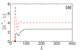
Figure 2: (Color online) $\beta=0.95\pi$, $\mbox{{Bo}}=0.005$. Solid lines are for $W\!e=0$ and dashed lines are for $W\!e=3$: (a) Bifurcation diagram for the norm $\|h^{*}-1\|$ against domain size $L$. The circles indicate the starting points for the continuations; (b) Pulse profiles for large $L$; (c) Shifted profiles $h^{*}-1$ for large $L$ shown on a logarithmic scale. Also included are dot-dashed lines showing inverse cube decay in $|x|$ for comparison purposes.

Figure 2 shows the results of numerical continuation for an obtuse inclination angle, $\beta=0.95\pi$, when $\mbox{{Bo}}=0.005$ and $W\!e=0$ and $3$. A Stuart-Landau analysis suggests that the bifurcation at $L=L_{+}=\pi/\kappa_{+}$, both for $W\!e=0$ and for $W\!e=3$, is supercritical, and the numerical results corroborate this. Both the norm and the speed converge to constants as $L$ increases. Also, for $W\!e=3$ both the norm and the speed are greater than those for $W\!e=0$. Both of the travelling waves are single-hump solitary pulses preceded by capillary ripples of decaying amplitudes. The left tail of the pulse for $W\!e=0$ decays monotonically to $1$ as $L\rightarrow-\infty$. However, for $W\!e=3$, the left tail exhibits a depression just upstream of the main hump before monotonically approaching $1$. Also, the amplitude of the pulse is larger when the electric field is switched on, while the amplitude of the ripples is not so significantly affected by the electric field. The semilog plots show that the electric field dramatically affects the decay rate of the tails, namely the decay is exponential when $W\!e=0$, but for $W\!e=3$ it becomes much slower in the far-field.

For acute inclination angles, the solutions of branches starting at the cut-off domain half-sizes, $L_{\pm}=\pi/\kappa_{\pm}$ do not always converge to single-hump solitary pulses. In fact, we find that only the solutions of the branch starting at $L_{-}$ converge to a single-hump solitary pulse when the electric Weber number is greater than a certain value that is greater than the linear instability threshold value $W\!e_{c}$. We demonstrate this in figures 3 and 4 showing the results for $\beta=0.25\pi$ and $\mbox{{Bo}}=0.01$ and for $W\!e=12.5$ and $13.5$, respectively. Both of these values of the electric Weber number are above the linear instability threshold, which is $W\!e_{c}\approx 11.89$ in this case. The bifurcations at $L=L_{+}$ and $L=L_{-}$ produce side branches which move toward larger and smaller values of $L$, respectively, for $W\!e=12.5$. This is again in agreement with a Stuart-Landau analysis. For $W\!e=12.5$, the points corresponding to the $L_{+}\approx 19.21$ and $L_{-}\approx 36.32$ are connected by a single branch of periodic travelling-wave solutions. For $W\!e=13.5$, there are two distinct solution branches emanating from the points corresponding to the $L_{+}\approx 15.80$ and $L_{-}\approx 44.18$, and both branches apparently extend to infinitely large values of $L$. Both side branches move immediately toward larger values of $L$ in agreement with a Stuart-Landau analysis. For both branches, the norm $\|h^{*}-1\|$ and the speed $c^{*}$ tend to constant values as $L$ increases. The wave profile in panel (b) apparently converges to a single-hump solitary pulse preceded by capillary ripples of decaying amplitude, as for the case of an obtuse inclination angle. Also, like for the obtuse inclination angle, the left tail of the pulse is not monotonically decaying. There is a depression upstream of the pulse, and only then the tail tends to $1$ monotonically as $x\rightarrow-\infty$. The wave profile in panel (c) does not correspond to a single-hump pulse. Instead, it has the shape of a double-hollow negative solitary pulse in the terminology of Chang and co-workers (Chang, 1994; Chang & Demekhin, 2002) and with capillary ripples upstream and an elevation downstream, and, moreover, it travels at a speed that is smaller than that for the single-hump pulse.

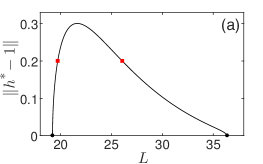
Figure 3: (Color online) $\beta=0.25\pi$, $\mbox{{Bo}}=0.01$, $W\!e=12.5$ (a) Bifurcation diagram for $\|h^{*}-1\|$ against domain size $L$. (b, c) Wave profiles with norm $\|h^{*}-1\|=0.2$, indicated by the left and right squares in (a), respectively.

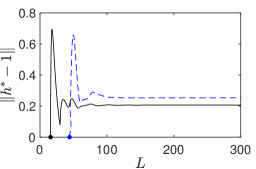
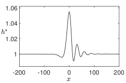
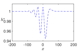
Figure 4: (Color online) $\beta=0.25\pi$, $\mbox{{Bo}}=0.01$, $W\!e=13.5$. (a) Bifurcation diagram for $\|h^{*}-1\|$ against domain size $L$. The solid and dashed lines show bifurcation branches emerging from $L_{+}=15.80$ and $L_{-}=44.18$, respectively. (b, c) Pulse profiles for large $L$ on the branches emerging from $L_{+}$ and $L_{-}$, respectively.

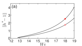
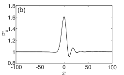
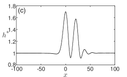
Figure 5: (Color online) $\beta=0.25\pi$, $\mbox{{Bo}}=0.01$. (a) Solution branch showing the norm $\|h^{*}-1\|$ against electric Weber number $W\!e$. (b, c) Pulse profiles at $W\!e=18$, indicated by the empty and filled circle symbols respectively in panel (a). The wave speeds are $c^{*}=2.22$ (b), $2.15$ (c).

Finally, to investigate in more detail the influence of an electric field on single-hump solitary pulses, we consider such a pulse for $\beta=0.25\pi$, $\mbox{{Bo}}=0.01$ on the domain $[-300,300]$, and perform continuation in the electric Weber number, $W\!e$. The results are shown in figure 5. The branches have turning points at $W\!e=W\!e^{\dagger}\approx 12.77$, which indicates that single-hump solitary pulses do not exist for $W\!e<W\!e^{\dagger}$. The lower part of the branch in panel (a) of figure 5 corresponds to single-hump pulses. The upper branch in panel (a) corresponds to double-hump pulses. Both for single- and double-hump pulses the norm and the speed monotonically increase as $W\!e$ increases.

A straightforward far-field analysis for the non-electrified case reveals that if $c^{*}>2\sin\beta$ we obtain monotonic decay on the upstream side of the pulse and non-monotonic, oscillatory decay on the downstream side of the tails. Referring back to the scales we have used to non-dimensionalise the problem, this inequality corresponds to the physical pulse speed being greater than the speed of small amplitude linear long waves, which themselves propagate at twice the surface speed of a flat film on an inclined plane, namely $2U_{0}\sin\beta$ (e.g. Benjamin, 1957). If instead $c^{*}<2\sin\beta$, we will have oscillatory decay on the upstream side of a pulse and monotonic decay on the downstream side.

With an electric field present, the decay becomes algebraic (see also Lin et al., 2015). Assuming that the pulse has a non-zero ‘mass’, i.e. $\int_{-\infty}^{\infty}(h^{*}-1)dx\neq 0$, it can be shown that $(h^{*}-1)\propto 1/x^{3}$ as $x\rightarrow\pm\infty$.

3.2 Weak-interaction theory for solitary pulses

We generalise the earlier work of Lin et al. (2015) to the case of the general one-dimensional evolution equation with translational symmetry, $\partial_{t}u=\partial_{x}(G[u])$, for some $G$ such that $G[h^{*}-\alpha]=0$, where $h^{*}\to\alpha$ as $|x|\to\infty$. The work of Lin et al. (2015) built on earlier studies by Elphick et al. (1990), Elphick et al. (1991), Balmforth (1995), Chang & Demekhin (2002) for the case of local equations. Certain technical details in these studies were re-examined by Pradas et al. (2011) and Tseluiko & Kalliadasis (2014).

We consider (7) in a frame moving with the speed $c^{*}$ of a pulse solution. We represent a solution of (7) as a superposition of $N$ well-separated quasi-stationary pulses located at $x_{1}(t)<\cdots<x_{N}(t)$ and a small overlap function $\hat{u}$. Suppressing the details in the interest of brevity, we obtain the dynamical system describing the locations of the pulses (see Lin et al., 2015)

$$\dot{x}_{k}=-\Pi_{k}\left[\partial_{x}\left(G\left[\sum_{|x_{i}-x_{k}|<b(\epsilon)}u_{i}\right]\right)\right],\qquad k=1,\,\ldots,\,N,$$ (10)

where $b(\epsilon)\gg\epsilon^{-1/p}$ is the range over which the interactions must be taken into account. Here, $\Pi_{k}$ is a projection operator defined by $\Pi_{k}[f]=\int_{-\infty}^{\infty}f\psi_{k}\,\mathrm{d}x$, where $\psi_{k}$ is the zero adjoint eigenfunction for the operator $\partial_{x}\circ\mathscr{D}_{u_{k}}G$ normalised so that $\int_{-\infty}^{\infty}u_{kx}\psi_{k}\,\mathrm{d}x=1$. Note that $\mathscr{D}_{u_{k}}G$ denotes the Fréchet derivative of operator $G$ at $u_{k}$. We note that in (10), for the case of an electrified film, it is necessary to include long-range interactions over more than just the immediately neighbouring pulses as a direct result of the algebraic decay of the pulse tails.

Let us consider a two-pulse system, $N=2$. From (10), we may derive the evolution equation for the pulse separation

$$\dot{l}=\tilde{P}(l),\qquad\tilde{P}(l)\equiv\int_{-\infty}^{\infty}\partial_{x}(G[u^{*}(x+l)-u^{*}(x-l)])\psi(x)\,\mathrm{d}x.$$ (11)

Depending on the initial condition, the two pulses may attract ($\tilde{P}(l)<0$) or repel ($\tilde{P}(l)>0$) each other. The pulses can also form bound states, the separation distances for which are zeros of $\tilde{P}(l)$. Figures 6(a) and 6(b) show $\tilde{P}(l)$ for $\beta=0.95\pi$ and $\mbox{{Bo}}=0.005$, and for $W\!e=0$ and $2.25$, respectively. Apparently, there exist infinitely many bound states for $W\!e=0$, while there exist only eight possible bound states for $W\!e=2.25$. To understand this, we note that for $W\!e=0$, it can be shown that as $l\to\infty$, $\tilde{P}$ decays either monotonically or in an oscillatory manner. If the decay is monotonic, there are zero or a finite number of positive solutions to $\tilde{P}(l)=0$ implying zero or a finite number of two-pulse bound states If the decay is oscillatory, there is a countably infinite number of solutions to $\tilde{P}(l)=0$, and, hence, an infinite number of two-pulse bound states.

We note that in the case of no electric field, the travelling-wave form of (7) is local and can be integrated once to yield a three-dimensional dynamical system. Then, a single-pulse solution corresponds to a homoclinic orbit in the three-dimensional phase space for this system. In such a case, the same conclusion on the number of bound states in existence can be reached using Shil’nikov’s theorem (see, for example, Glendinning & Sparrow, 1984). This gives a criterion for the number of subsidiary homoclinic orbits which correspond to two-pulse bound states, which exactly coincides with that found via the monotonic/oscillatory decay argument given above. However, when $W\!e>0$, the travelling-wave form of (7) is non-local and the Shil’nikov-type approach is not applicable. Instead, the weak-interaction theory developed here can be used to analyse bound states. Then, it can be shown that $\tilde{P}(l)$ decays monotonically algebraically to zero as $l\rightarrow\infty$, and hence there exist only a finite number of two-pulse bound states.

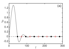
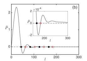
Figure 6: (Color online) $\tilde{P}(l)$ against $l$ for $\beta=0.95\pi$ and $\mbox{{Bo}}=0.005$, and for (a) $W\!e=0$ and (b) $W\!e=2.25$. Bound states are marked as filled circles (stable) and empty circles (unstable). The inset in panel (b) shows the behaviour for large $l$, which becomes monotonic.

To validate the theoretically predicted pulse dynamics (11), we numerically simulated the dynamics of a two-pulse system using a superposition of two pulses as an initial condition for various parameter values and initial separation distances. We found excellent agreement between the simulations and the theory. Similarly good agreement was found for simulations with three and four pulses. For a physical explanation of pulse attraction and repulsion, see Duprat et al. (2009).

4 Fully nonlinear solutions for Stokes flow

We now study fully nonlinear pulse solutions at zero Reynolds number. We discuss the case of a perfect conductor film, that is $\varepsilon_{p}\to\infty$. The extension to the case of a liquid dielectric is straightforward (e.g. Tseluiko et al., 2008).

We first reformulate the problem using the boundary-integral method. The flow is assumed to be periodic in $x$ with half-period $L$. We decompose the steady flow velocity $\boldsymbol{u}$ and stress tensor $\sigma$ into a basic flow part and a disturbance part, writing $\boldsymbol{u}=\boldsymbol{u}^{B}+\boldsymbol{u}^{D}$ and $\mbox{\boldmath{$\sigma$}}=\mbox{\boldmath{$\sigma$}}^{B}+\mbox{\boldmath{$\sigma$}}^{D}$. In the travelling frame, the basic flow details are

$$\boldsymbol{u}^{B}=(y(2-y)\sin\beta-c^{*},0),\quad\mbox{\boldmath{$\sigma$}}^{B}=-p_{a}\boldsymbol{I}+2(1-y)\begin{pmatrix}-\cos\beta&\sin\beta\\ \sin\beta&-\cos\beta\end{pmatrix},$$ (12)

where $p_{a}$ is the constant dimensionless ambient pressure above the film, and the remaining symbols have been defined in § 3. Setting $c^{*}=0$ in (12), we recover the classical Nusselt solution for unidirectional flow down an inclined plane. We note that according to the decomposition described, the disturbance velocity $\boldsymbol{u}^{D}$ vanishes at the wall, $y=0$.

Following the boundary-integral formalism, we obtain the integral equation for the disturbance velocity and disturbance traction $\boldsymbol{f}^{D}\equiv\mbox{\boldmath{$\sigma$}}^{D}\cdot\boldsymbol{n}$ at a point $\boldsymbol{x}_{0}=(x_{0},y_{0})$ located on the free surface,

$$2\pi u_{j}^{D}(\boldsymbol{x}_{0})=-\int_{F}G_{ij}(\boldsymbol{x},\boldsymbol{x}_{0})f_{j}^{D}(\boldsymbol{x})\,\mbox{d}l(\boldsymbol{x})+\mathrm{p.v.}\int_{F}u_{i}^{D}(\boldsymbol{x})T_{ijk}(\boldsymbol{x},\boldsymbol{x}_{0})n_{k}(\boldsymbol{x})\,\mbox{d}l(\boldsymbol{x}),\,\,$$ (13)

where p.v. denotes the principal value, $F$ denotes one period of the free surface, $l$ is arc length along $F$, $\boldsymbol{n}$ is the unit normal at the free surface pointing into the fluid, $G_{ij}(\boldsymbol{x},\boldsymbol{x}_{0})$ is the periodic Green’s function for Stokes flow, which vanishes when $\boldsymbol{x}$ is located on the wall at $y=0$, and $T_{ijk}(\boldsymbol{x},\boldsymbol{x}_{0})$ is the corresponding stress tensor. Closed form expressions for $\boldsymbol{G}$ and $\boldsymbol{T}$ can be found in Pozrikidis (2002). The kinematic condition at the free surface in the travelling frame requires that

$$\boldsymbol{u}^{D}\cdot\boldsymbol{n}=-\boldsymbol{u}^{B}\cdot\boldsymbol{n}.$$ (14)

Following the boundary-integral method for Laplace’s equation (e.g. Pozrikidis, 2002), we obtain the integral equation for the electric potential,

$$\begin{array}[]{rl}\displaystyle\frac{1}{2}\varphi_{2}(\boldsymbol{x}_{0})=-\int_{F}G(\boldsymbol{x},\boldsymbol{x}_{0})\boldsymbol{n}(\boldsymbol{x})\cdot\nabla\varphi_{2}(\boldsymbol{x})\>\mathrm{d}l(\boldsymbol{x})-y_{0}+B,\end{array}$$ (15)

where $B$ is an a priori unknown constant, and $G$ is the singly-periodic upward-biased Green’s function with half-period $L$, given by (see Pozrikidis, 2002, p. 261)

$$G(\boldsymbol{x},\boldsymbol{x}_{0})=-\frac{1}{4\pi}\log\left[2\left(\cosh[k(y-y_{0})]-\cos[k(x-x_{0})]\right)\right]-\frac{y-y_{0}}{4L}.$$ (16)

By integrating Laplace’s equation for $\varphi$ over one period of the semi-infinite region above $F$, we obtain the integral condition

$$\int_{F}\boldsymbol{n}\cdot\nabla\varphi_{2}\>\mbox{d}l(\boldsymbol{x})=2L,$$ (17)

which is to be satisfied along with (15).

The problem for the electric field and the problem for the fluid flow are coupled together via the dynamic stress boundary condition at the free surface,

$$\boldsymbol{f}^{D}=-\boldsymbol{f}^{B}-\frac{\kappa}{\mbox{{Bo}}}\boldsymbol{n}+W\!e|\nabla\varphi|^{2}\boldsymbol{n}.$$ (18)

To complete the formulation, we specify two more conditions akin to those imposed for the long-wave model. First, we remove the translational invariance by imposing the condition $h^{*}_{x}=0$ at $x=0$, and to break the ‘volume’ symmetry, we impose the condition $h^{*}=1$ at $x=L$. By fixing the location of the wave maximum and the film height in this way, we efficiently compute pulse solutions (where they exist) by increasing $L$.

With these final two conditions, the coupled integral formulation comprising (13), (15) and (17), together with the kinematic condition (14) and the dynamic stress condition (18) are solved numerically using the boundary-element method by discretising one period of the a priori unknown free surface, $F$, with a sequence of $N$ connected straight elements and treating the unknown variables as constants over the elements. In this way, we derive a set of nonlinear algebraic equations to be solved using Newton’s method for these unknown constant element values, the free-surface profile $h^{*}$ and the wave speed $c^{*}$. Full details of the implementation ofthe method are provided by Tseluiko et al. (2008) and, in the interest of brevity, we do not repeat them here.

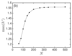
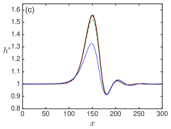
Figure 7: (Color online) Stokes flow computations with $\beta=0.95\pi$, $\mbox{{Bo}}=0.005$, $W\!e=0$: (a) Travelling-wave branch for Stokes flow showing the wave height, $\max(h^{*})-\min(h^{*})$, against $L$, computed using $N=300$ boundary elements. (b) Numerical convergence for $L=150$ showing $\max(h^{*})$ against $N$. (c) Pulse profile for $L=150$ and $N=300$ (solid line) with the long-wave predictions using (7) and (19) (dashed, dot-dashed lines, respectively) and the KS prediction (thin solid line). The wave speed is $c^{*}=0.457$ (boundary-element solution) and $c^{*}=0.449$ (long-wave solution to equation 7) and $c^{*}=0.392$ (KS equation 8).

A standard normal-mode analysis for small-amplitude periodic waves (see Blyth, 2008) reveals that the cut-off wavenumber coincides with that found from the long-wave analysis. The properties of the neutral mode are used to construct an initial guess for the Newton iterations and to latch onto the travelling-wave solution branch. This is followed using continuation in $L$, and in the case where $L$ may be increased indefinitely, we are able to compute solitary-pulse solutions. The solution space is determined by the three dimensionless parameters Bo, $We$ and $\beta$ introduced in § 3.

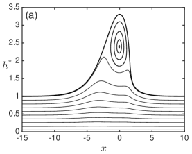
Figure 8: (Color online) Stokes flow calculation for $\beta=0.75\pi$ with $\mbox{{Bo}}=0.3$ and $W_{e}=0$, and with $L=16.0$ and $N=400$. (a) Pulse profile and streamlines. (b) Logarithm of the pulse profile (solid line) with broken lines of gradient $0.576$ in $x<0$ and $-0.741$ in $x>0$ corresponding to the decay rate predictions (see Appendix A). The wave speed is $c^{*}=3.82$.

We begin by computing fully nonlinear pulse solutions for no electric field, setting $W\!e=0$. In figure 7(a), we show the results of a sequence of calculations for increasing domain size $L$. The wave height approaches a constant value, and a pulse solution is obtained, at around $L\approx 200$. It was found that $N=300$ boundary elements were sufficient to obtain an accurate wave solution. The numerical convergence is demonstrated in figure 7(b), which shows the variation of the pulse maximum with the number of boundary elements $N$ at $L=150$. The pulse itself is shown in figure 7(c) with a thick solid line. The long-wave prediction based on (7) and the weakly-nonlinear prediction based on the KS equation (8) are also shown in this figure. The pulse speed is found to be $c^{*}=0.457$ for the boundary-element calculation and $c^{*}=0.449$ for the long-wave calculation, and so there is reasonable agreement between the two values.

Notably, the performance of the KS equation is rather poor, even at this small value of the Bond number. Nevertheless, we have confirmed that the long-wave and KS solutions converge as the Bond number is further reduced. Evidently the long-wave and boundary-element calculations agree very well with a small discrepancy around the maximum of the pulse. The discrepancy is significantly reduced by including higher-order terms in the long-wave model equation; specifically including second-order terms in the derivation we obtain the extended form of (7),

$$h_{t}+q_{x}=0,$$ (19)

where $q=q_{0}+q_{1}+q_{2}$, with $q_{0}=O(1)$, $q_{1}=O(\delta)$, $q_{2}=O(\delta^{2})$. Specifically,

$$q_{0}=\frac{2}{3}(\sin\beta)h^{3}-\frac{2}{3}(\cos\beta)h^{3}h_{x}+\frac{1}{3\mbox{{Bo}}}h^{3}h_{xxx}+\frac{2W\!e}{3}\,h^{3}\,\mathcal{H}[h_{xx}],$$ (20)

and $q_{1}=F_{1}+\mathcal{E}_{1}$, where $F_{1}$ contains terms all of which vanish when $Re=0$, and

$$\mathcal{E}_{1}=\frac{1}{3}W\!e\,h^{3}\left(E_{2x}+2h_{x}h_{xx}\right),$$ (21)

(see Tseluiko & Papageorgiou, 2010) and

$$q_{2}= h^{3}\Bigg{(}\sin\beta\left(2hh_{xx}+\frac{14}{3}h_{x}^{2}\right)-2\cos\beta\Big{(}4hh_{x}h_{xx}+\frac{3}{5}h^{2}h_{xxx}+\frac{7}{3}h_{x}^{3}\Big{)}$$

$$+\frac{1}{\mbox{{Bo}}}\left(3hh_{x}h_{xxxx}-h_{x}h_{xx}^{2}+\frac{11}{6}h_{x}^{2}h_{xxx}+hh_{xx}h_{xxx}+\frac{3}{5}h^{2}h_{xxxxx}\right)\Bigg{)}+F_{2}+\mathcal{E}_{2},$$ (22)

where $F_{2}$ contains terms all of which vanish when $Re=0$. The electric-field contribution $\mathcal{E}_{2}$ must be found by considering the electric field problem at the appropriate order, but is not needed for the present non-electrified case. Equation (19) is valid provided that $\mbox{{Bo}}=O(\delta^{2})$, $W\!e=O(\delta^{-1})$, $\cot\beta=O(\delta^{-1})$ and $Re=O(1)$. The pulse solution to this equation is shown in figure 7(c) with a dot-dashed line which almost coincides with the thick solid line representing the boundary-element solution.

The pulse profile in figure 7(c) decays monotonically on the upstream side and has an oscillatory decay on the downstream side. Since the pulse speed is greater than the speed of linear long waves, namely $2\sin\beta=0.313$, this is consistent with the predictions of the decay rate calculations discussed in Appendix A. These calculations predict that when the Bond number is not small the decay is monotonic both upstream and downstream of the pulse maximum. Figure 8(a) shows the pulse profile for $\mbox{{Bo}}=0.3$ and $\beta=0.75\pi$. The pulse speed is $c^{*}=3.82$. Evidently the decay is monotonic on both sides of the pulse. For these parameter values the calculation described in Appendix  A yields the upstream and downstream decay rates $0.576$ and $-0.741$, respectively, and these show good agreement with the profile calculated using the boundary-element method, as can be seen in Figure 8(b). The figure also shows streamlines inside the film in a frame of reference travelling at the speed of the pulse. These indicate the presence of a trapped eddy in the main part of the pulse. Solitary wave eddies have recently been observed experimentally on a gravity-driven film at non-zero Reynolds number by Reck & Aksel (2015).

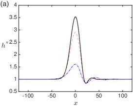
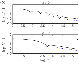
Figure 9: (Color online) Electrified Stokes flow computation for $\beta=0.95\pi$, $\mbox{{Bo}}=0.005$, $We=6.25$, and $L=250$, $N=500$. (a) Pulse profile (solid line) with the long-wave prediction (dashed line) and the KS prediction (dot-dashed line). (b) A $\log$-$\log$ plot of the pulse profile in $x>0$ and $x<0$ showing algebraic decay in the far-field with the expected slope (dashed line) according to the asymptotic theory presented in Appendix A. The wave speed is $c^{*}=1.09$ (boundary-element solution) and $c^{*}=0.88$ (long-wave solution) and $c^{*}=0.46$ (KS solution).

An electrified solitary-pulse solution is shown in figure 9(a). According to the theory of Appendix A, the far-field decay of an electrified pulse is algebraic and so a wide computational domain and a large number of boundary elements are needed for an accurate computation. The prediction of the long-wave model equation (7) is also shown in the figure with a broken line. Once again, we see that there is good agreement over most of the pulse profile except near to the main peak. The visible difference between the Stokes calculation and the long-wave one at the pulse maximum is exacerbated in the presence of the electric field (compare the results in figure 7c). As for the non-electrified case studied in figure 7(b, c), we would expect the agreement to improve on using the extended long-wave model equation (19). However, this would require computation of the corresponding electric field contribution $\mathcal{E}_{3}$. The decay rate of the pulse tails as $|x|\to\infty$ is investigated in figure 9(b). The broken lines shown in the figure indicate the algebraic decay rate expected from the asymptotic theory of Appendix A. The excellent agreement provides strong evidence of algebraic decay in the far-field and lends strong credence to the decay rate predicted by the asymptotic theory. The pulse speed determined from the boundary-element solution is $c^{*}=1.09$; this compares with $c^{*}=0.88$ obtained from the long-wave theory. We note that the pulse travels faster in the presence of the electric field. This trend is in line with the long-wave theory.

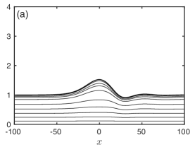
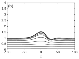
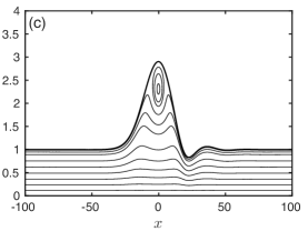
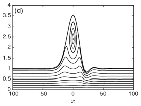
Figure 10: (Color online) Streamline patterns in a frame moving at the pulse speed for the case $\beta=0.95\pi$ with $\mbox{{Bo}}=0.005$: (a, b) $W\!e=0$, (c, d) $W\!e=6.25$. We note that (b) and (d) are results for Stokes model while (a) and (c) are for long-wave model. The pulse profiles are shown with a thick line and the streamlines with thin lines.

Figure 10 depicts the streamline patterns for $\beta=0.95\pi$ and $\mbox{{Bo}}=0.005$ in a frame moving with the pulse for $W\!e=0$ (panels a and b) and $W\!e=6.25$ (panels c and d). Panels (a) and (c) show results for the long-wave model and panels (b) and (d) show the results of boundary-element calculations. The two different models give broadly similar results. Notably the electric field generates an eddy/recirculation zone inside the hump so that a quantity of fluid is transported along with the pulse.

Next, we discuss the computation of bound states for the Stokes equations. We construct an initial guess made from a superposition of a converged pulse solution and a duplicate of the same pulse separated by a nominated distance, $l$, which is taken to coincide with that given by the long-wave theory of § 3.2. A good initial guess is required as the convergence of the Newton iterations is sensitive to the separation distance. Figure 11 shows four bound-state solutions for the case $\mbox{{Bo}}=0.005$ and $\beta=0.95\pi$ for $W\!e=0$ or $2.25$. For these parameter values and for the non-electrified case, the long-wave theory predicts the existence of twelve bound states with separation distances: $47.30$, $69.74$, $94.13$, $117.62$, $141.38$, $165.05$, $188.75$, $212.42$, $236.37$, $260.01$, $283.71$, $307.41$. We computed only a subset of these shown in the figure. The accuracy of each calculation was confirmed by varying the number of boundary elements and the size of the computational domain. For each case, the wave speed $c^{*}$ predicted by the boundary-element computation and by the long-wave theory are given in table 1. Evidently, the two are in good agreement. The wave speed is quite a lot smaller for a bound-state than for a solitary pulse travelling alone. We also note that for both the boundary-element and the long-wave calculations, the separation distances, which in the case of Stokes flow are measured as the distance from maximum to maximum, decrease as the electric field intensity is increased.

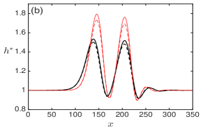
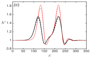
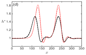
Figure 11: (Color online) Stokes flow bound-state computations for $\beta=0.95\pi$, $\mbox{{Bo}}=0.005$ (with $L=175$, $N=500$) for $We=0$ (thick solid lines) and $We=2.25$ (thin solid lines). The separation distances from maximum to maximum are (with electrified values in brackets): (a) $56.5$ ($50.5$), (b) $67.0$ ($60.0$), (c) $96.0$ ($84.0$), and (d) $117.0$ ($111.0$). The long-wave predictions for non-electrified (electrified) flows are shown with thick (thin) dashed lines. The long-wave bound-state separation distances are (with electrified values in brackets): (a) $47.3$ ($43.4$), (b) $69.7$ ($62.5$), (c) $94.1$ ($83.6$), and (d) $117.6$ ($111.2$). The wave speeds are given in table 1.

Figure label			$c^{*}_{BEM}$			$c^{*}_{LW}$				Figure label			$c^{*}_{BEM}$			$c^{*}_{LW}$
11(a)			$0.38$ ($0.40$)			$0.38$ ($0.40$)				11(c)			$0.45$ ($0.52$)			$0.44$ ($0.51$)
11(b)			$0.46$ ($0.53$)			$0.45$ ($0.51$)				11(d)			$0.44$ ($0.48$)			$0.45$ ($0.47$)

Table 1: Wave speeds for the bound states in figure 11 quoted for the Stokes flow boundary-element computations ($c^{*}_{BEM}$) and for the long-wave model, ($c^{*}_{LW}$). Values in brackets are for the electrified cases with electric Weber numbers $W\!e$ as given in the caption to figure 11.

In § 3.1, using the long-wave model, we found that in the case of electrified flow at an acute inclination angle, the travelling-wave branches which emerge from the two neutral stability points at $L=L_{\pm}$ either connect to form a continuous hoop from one to the other or else each branch continues independently to large $L$ ultimately producing a solitary-pulse solution. Figures 12 and 13 demonstrate that the same behaviour is observed for Stokes flow. These two figures use the same parameter values as for the long-wave calculations in figures 3 and 4. In figure 12 ($W\!e=12.5$), we see that the neutral stability points at $L_{+}\approx 19.21$ and $L_{-}\approx 36.32$ are connected by a single continuous travelling-wave branch. Sample profiles along the branch are also shown in the figure. In figure 13 ($W\!e=13.5$), two independent branches emerge from the neutral points at $L_{+}\approx 15.80$ and $L_{-}\approx 44.18$, and continue until pulse solutions are finally attained for large $L$. The pulse profiles are also shown in the figure.

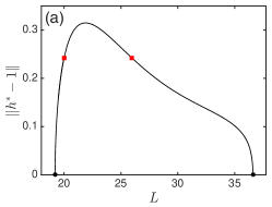
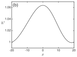
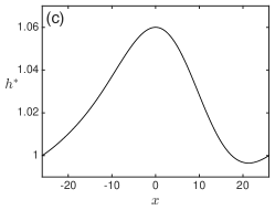
Figure 12: (Color online) Stokes flow computations for $\beta=0.25\pi$, $\mbox{{Bo}}=0.01$, $W\!e=12.5$: (a) Bifurcation diagram for $\|h^{*}-1\|$ against $L$. (c, d) Wave profiles with $\|h^{*}-1\|=0.2427$, indicated by the left and right squares in (a), respectively.

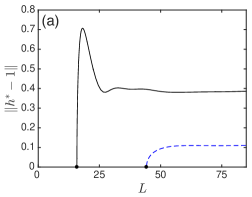
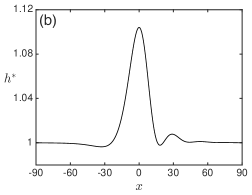
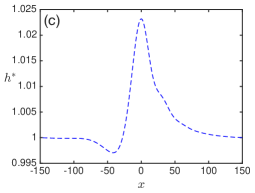
Figure 13: (Color online) Stokes flow computations for $\beta=0.25\pi$, $\mbox{{Bo}}=0.01$, $W\!e=13.5$: (a) Bifurcation diagram for the $\|h^{*}-1\|$ against $L$ with branches emerging from $L_{+}\approx 15.80$ (solid line) and $L_{-}\approx 44.18$ (dashed line). (c, d) Pulse profiles for large $L$ on the branches emerging from $L_{+}$ and $L_{-}$, respectively.

We present in figure 14 some examples of negative solitary pulses. In the non-electrified case shown in figure 14(a), the boundary-element solution is compared with the prediction for the same wave using the long-wave model. It is noticeable that, as for the elevation pulse shown in figure 7(c), the greatest discrepancy between the boundary-element and long-wave calculations is observed at the largest peak. The pulse speed is $c^{*}=0.259$ for the Stokes calculation and $c^{*}=0.257$ for the long-wave calculation. This is smaller than the speed of linear long waves $2\sin\beta=0.313$. Evidently the negative pulse is also travelling more slowly than its elevation pulse counterpart for the same Bond number and inclination angle shown in figure 7(c), whose speed is $c^{*}=0.457$.

Figure 14(b) shows the effect of increasing the electric field intensity. Similar to the elevation pulses studied above, the electric field tends to deepen the depression and heighten the amplitude of the downstream oscillations. The electric field also tends to lower the speed of the wave (values for the wave speed are quoted in the figure caption).

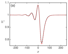
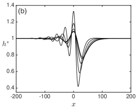
Figure 14: (Color online) Negative pulse profiles for Stokes flow with $\mbox{{Bo}}=0.005$, $\beta=0.95\pi$ (with $L=250$, $N=500$). (a) $W\!e=0$: boundary-element solution (solid line) and long-wave solution (dashed line). (b) Boundary-element solutions for $We=0$, $1.0$, $4.0$, $9.0$ and $16.0$ with the depth of the main trough increasing with $W\!e$. The wave speeds are, respectively, $c^{*}=0.259$, $0.255$, $0.242$, $0.217$, $0.183$.

5 Absolute/convective instability of pulse solutions

We now discuss the stability of the pulse solutions calculated in the previous sections. In particular, we classify pulses as being either convectively unstable or absolutely unstable. Suppose first that the flow supports pulses which are convectively unstable. Since such a pulse can tolerate localised disturbances, in time-dependent solutions we would see the flow ultimately evolve into a state with an array of such pulses undergoing weak interactions. Suppose instead that the pulses supported by the flow are absolutely unstable. These can be destroyed by localised disturbances and consequently we would expect to see highly irregular dynamics in a general time-dependent simulation. For further discussion see Chang et al. (1995); Chang & Demekhin (2002).

To study stability, we linearise about a pulse state by imposing a small perturbation in a reference frame which is moving with the pulse at speed $c^{*}$, writing

$$h(x,t)=h^{*}(x)+\eta(x,t),$$ (23)

where $\eta(x,t)$ is a small perturbation localised in space, and $h^{*}\to 1$ as $|x|\to\infty$.

We consider first long-wave pulses which are solutions of the model equation (7). Substituting (23) into (7), written in a frame moving at the pulse speed $c^{*}$, and ignoring nonlinear terms, we obtain

$$\partial_{t}\eta=\mathcal{L}[\eta],\qquad\mathcal{L}\eta=(a_{0}\eta+a_{1}\eta_{x}+a_{2}\mathcal{H}[\eta_{xx}]+a_{3}\eta_{xxx})_{x}$$ (24)

with

$$\displaystyle a_{0}(x)=c^{*}-2(\sin\beta)h^{*2}+2(\cos\beta)h^{*2}h^{*}_{x}-\frac{1}{\mbox{{Bo}}}h^{*2}h^{*}_{xxx}-2W\!e\>h^{*2}\mathcal{H}[h^{*}_{xx}],$$

$$\displaystyle a_{1}(x)=\frac{2\cos\beta}{3}h^{*3},\qquad a_{2}(x)=-\frac{2}{3}W\!e\>h^{*3},\qquad a_{3}(x)=-\frac{1}{3\mbox{{Bo}}}h^{*3}.$$ (25)

The solution of (24) can be written as (e.g. Chang et al., 1996; Lin et al., 2015)

$$\eta(x,t)=\sum_{i}\mathrm{e}^{\lambda_{i}t}B_{i}\phi_{i}(x)+\int_{-\infty}^{\infty}\mathrm{e}^{\sigma(\kappa)t}B(\kappa)\phi(x,\kappa)\>\mathrm{d}\kappa,$$ (26)

where the summation is over all the isolated eigenvalues $\lambda_{i}$ (the discrete spectrum) with corresponding eigenfunctions $\phi_{i}(x)$, that is the functions belonging to the null space of $\lambda_{i}I-\mathcal{L}$, and $B_{i}$ are constants. In fact, for the given model, we find numerically that there is only one isolated eigenvalue, which is real and negative. The same happens, for example, for the gKS equation Chang et al. (1996); Tseluiko & Kalliadasis (2014). In the second integral, $\sigma(\kappa)$ is the essential spectrum of $\mathcal{L}$ which we find coincides precisely with the spectrum for a flat film as is the case with the established theory for ordinary differential operators Edmunds & Evans (1987); Pego & Weinstein (1992). For a flat film of unit thickness this is given by

$$\sigma=(c^{*}-2\sin\beta)\mathrm{i}\kappa-\frac{2\cos\beta}{3}\>\kappa^{2}+\frac{2W\!e}{3}\>|\kappa|^{3}-\frac{\kappa^{4}}{3\mbox{{Bo}}},$$ (27)

where $\kappa\in\mathbb{R}$. In (26), $\phi(x,\kappa)$ are functions in to the null space of $\sigma I-\mathcal{L}$, and (27) implies that $\sigma(-\kappa)=\overline{\sigma(\kappa)}$ and also $\phi(x,-\kappa)=\overline{\phi(x,\kappa)}$, where the overline denotes complex conjugation. For a real perturbation $\eta$, the coefficients $B(\kappa)$ satisfy $B(-\kappa)=\overline{B(\kappa)}$.

Since the discrete spectrum contains only $\lambda_{1}$, and $\lambda_{1}$ is negative, the first term in (26) decays to zero as $t\to\infty$, and the convective/absolute nature of the instability is determined by the second, integral term, which we label $I_{c}$. From (27), if $W\!e^{2}\mbox{{Bo}}\leq 2\cos\beta$ then $\mathrm{Re}(\sigma)\leq 0$ and the flow is spectrally stable. However, if $W\!e^{2}\mbox{{Bo}}>2\cos\beta$ then $\mathrm{Re}(\sigma)>0$ if $|\kappa|\in(\kappa_{1},\kappa_{2})$, where

$$\kappa_{1} =\left\{\begin{array}[]{lll}\kappa_{-}&\mbox{if}&\phantom{\pi/}0<\beta\leq\pi/2\\ 0&\mbox{if}&\pi/2<\beta<\pi\end{array}\right.,\qquad\kappa_{2}=\kappa_{+},$$ (30)

where $\kappa_{\pm}$ are given in (9), and the flow is spectrally unstable. When the flow is unstable, we can determine the nature of the instability by looking to see if it is possible to deform the contour of integration for $I_{c}$ so that it is entirely contained inside the region of the complex $\kappa$ plane where $\mathrm{Re}(\sigma)<0$. If this is possible, then the instability is convective and otherwise the instability is absolute. However, $\sigma(\kappa)$ is not analytic in the complex $\kappa$ plane because of the $|\kappa|^{3}$ term in (27) and so the classical approach of Huerre & Monkewitz (1990) cannot be applied directly. To proceed, we note that we can rewrite $I_{c}$ as (see Lin et al., 2015; Vellingiri et al., 2015) $I_{c}=2\,\mathrm{Re}(K(x,t))$, where $K(x,t)=\int_{0}^{\infty}\mathrm{e}^{\sigma^{+}(\kappa)t}B(\kappa)\phi(x,\kappa)\>\mathrm{d}\kappa$, where $\sigma^{+}(\kappa)$ is given by (27) with $|\kappa|^{3}$ replaced by $\kappa^{3}$ and is an analytic function in the entire complex $\kappa$ plane. Furthermore, it is sufficient to consider the range of integration where $\mathrm{Re(\sigma^{+}})>0$ and examine the integral

$$K_{1}(x,t)=\int_{\kappa_{1}}^{\kappa_{2}}\mathrm{e}^{\sigma^{+}(\kappa)t}B(\kappa)\phi(x,\kappa)\>\mathrm{d}\kappa.$$ (31)

Since the integrand is analytic in the $\kappa$ plane, we may deform the contour of integration into any path $\Gamma$ connecting $\kappa_{1}$ and $\kappa_{2}$. The case of convective instability, in which the deformed contour $\Gamma$ lies entirely within a region with $\mbox{Re}\>\sigma^{+}(\kappa)<0$, is shown in figure 15(a). The case of absolute instability, for which the contour $\Gamma$ must pass through a region with $\mbox{Re}\>\sigma^{+}(\kappa)>0$, is shown in figure 15(c). The transition from convective to absolute instability under a continuous parameter change must happen by passing through the situation illustrated in figure 15(b) where the two lines on which $\mbox{Re}\,\sigma^{+}(\kappa)=0$ have pinched together at a saddle point, where $\mbox{d}\sigma^{+}/\mbox{d}\kappa=0$ (note that since $\sigma^{+}$ is analytic, points where $\mbox{d}\sigma^{+}/\mbox{d}\kappa$ vanishes are necessarily saddle points).

Figure 15: (Color online) Illustration of the change from (a) convective instability to (c) absolute instability. The solid lines shows where $\mbox{Re}\>\sigma^{+}(\kappa)=0$, and the broken line shows the integration contour $\Gamma$. Regions with $\mbox{Re}\>\sigma^{+}(\kappa)>0$ and $\mbox{Re}\>\sigma^{+}(\kappa)<0$ are shown with a $+/-$ respectively. The black dot indicates a saddle point.

Following the above discussion, to identify the transition from convective to absolute instability, we seek the parameter values for which $\mbox{Re}\>\sigma^{+}(\kappa)=0$ and $\mbox{d}\sigma^{+}/\mbox{d}\kappa=0$ at the relevant saddle point. To achieve this, we first take a pulse solution and solve the cubic equation $\mbox{d}\sigma^{+}/\mbox{d}\kappa=0$ to find the relevant saddle point (by scrutinising the contours) in the $\kappa$ plane. We then adjust $W\!e$ until $\mbox{Re}\>\sigma^{+}(\kappa)=0$ is satisfied. We may then continue in any desired parameter to trace out the transition boundary. Figure 16 shows the boundary between absolute and convective instability in the $(\mbox{{Bo}},W\!e)$ plane for a range of values of the inclination angle $\beta$. Evidently for fixed Bond number Bo, the flow is either convectively unstable for any value of $W\!e\geq 0$, or else as $W\!e$ increases it undergoes a transition from absolute to convective instability, and we, therefore, expect that sufficiently strong electric field should have a regularising effect on the dynamics. From the physical point of view, this can be explained as follows. The electric field has a destabilising effect on the flow, and results in the generation of larger-amplitude pulses. The speed of the pulses is also amplified by the electric field. If the electric field becomes sufficiently strong, the pulses become sufficiently fast so that they can escape expanding wave packets generated by localised disturbances. As a result, the pulses become convectively unstable.

Our results are consistent with those found by Lin et al. (2015) for the non-local KS equation (8), which supports pulse solutions which are absolutely unstable for any $W\!e$ Lin et al. (2015). This is consistent with the findings shown in figure 16: for any Bond number there is a transition from absolute to convective instability as the Weber number is increased, and the smaller the Bond number is the larger the Weber number at which the transition occurs.

Next, we turn our attention to a travelling pulse that is a solution to the full Stokes equations, as discussed in § 4. For a disturbance $\eta(x,t)$, which is superimposed onto a pulse solution, as for the long-wave case, the solution to the linearised stability problem may be written in the form (26). For the present purposes, we will assume that the discrete spectrum does not contain any eigenvalues which lie in the right half plane; consequently the first term in (26) decays to zero as $t\to\infty$ and, the convective/absolute nature of the instability is determined by study of the second term. As for the long-wave case the nature of the instability hinges on the ability to deform the contour of integration of the integral term $I_{c}$, as discussed in figure 15.

All of the elevation boundary-element pulse solutions for Stokes flow computed in § 4, both electrified and non-electrified (see figures 7c, 8a and 9a), are found to be convectively unstable. The negative pulse solutions presented in figure 14 are all absolutely unstable.

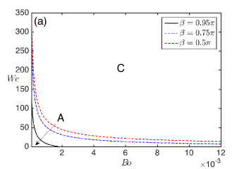
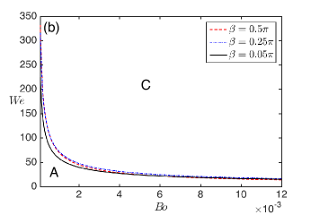
Figure 16: (Color online) Regions of convective (C) and absolute (A) instability in the $(\mbox{{Bo}},We)$ plane for a range of inclination angles for the long-wave model (24): (a) angles $\beta=0.5\pi,\,0.75\pi,\,0.95\pi$ and (b) angles $\beta=0.05\pi,\,0.25\pi,\,0.5\pi$.

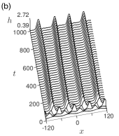
Figure 17: Time-dependent solutions of (7) for $\beta=0.75\pi$, $\mbox{{Bo}}=0.002$: (a) $W\!e=0$ and (b) $W\!e=62$, The top panels show the time evolution in a frame moving at speed (a) $1.4$ and (b) $2.22$, and the lower panels show the evolution of the norm $\|h-1\|$.

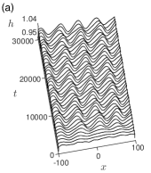
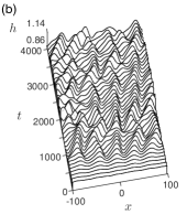
Figure 18: Time-dependent solutions of (7) for $\beta=0.25\pi$, $\mbox{{Bo}}=0.01$: (a) $W\!e=12.5$, (b) $W\!e=14.5$, (c) $W\!e=26$. The top panels show the time evolution of the solution in a frame moving at speed (a, b) $1.4$ and (c) $2.08$. The lower panels show the evolution of the norm $\|h-1\|$.

5.1 Time-dependent simulations

We have confirmed the predictions of the absolute/convective instability analysis of the long-wave model carried out above by conducting time-dependent simulations of (7). In each case, the initial condition was chosen to be comprised of a superposition of the first few Fourier modes with randomly assigned amplitudes. Figures 17 and 18 show the results of simulations for the obtuse inclination angle $\beta=0.75\pi$, in which case gravity is destabilising, and the acute inclination angle $\beta=0.25\pi$, when gravity is stabilising, respectively. The former set of simulations was conducted at $\mbox{{Bo}}=0.002$ while the latter set was done with $\mbox{{Bo}}=0.01$. For each of the simulations we show the time evolution of the film profile in the leftmost panel, and the final profile at the end of the simulation and evolution of the norm $\|h-1\|$ in the top and bottom rightmost panels, respectively. For the obtuse inclination angle, as can be seen in panel (a) of figure 17, non-trivial dynamics is observed even in the absence of an electric field due to the destabilising effect of gravity, and the dynamics remains highly irregular throughout the simulation. This is in agreement with the results shown in figure 16(a) which predicts that pulse solutions are absolutely unstable at this value of the electric Weber number. However, the dynamics becomes regularised when an electric field of sufficient intensity is introduced. This is demonstrated in panel (b) of figure 17 for the electric Weber number $W\!e=62$. The film surface evolves relatively quickly into an array of weakly interacting pulses. Although the norm reaches a plateau by about $t\approx 200$, the flow remains time-dependent as the pulses continue to rearrange their relative positions through weak attractions and repulsions.

For an acute inclination angle, a sufficiently strong electric field is required to produce non-trivial dynamics. For the case shown in figure 18, we see that at relatively low electric field strength ($W\!e=12.5$ in panel a), the film surface exhibits a nearly periodic modulated wave train during the time simulation. Pulses are not observed until the electric field strength exceeds a critical value in agreement with our earlier finding shown in figure 5, which predicts that pulses are only present when $W\!e>12.77$. Although pulses should theoretically exist at the Weber number considered in panel (b), namely $14.5$, they are absolutely unstable according to the analysis of § 5 (see figure 16(b); for $\mbox{{Bo}}=0.01$ and $\beta=0.25\pi$ the threshold between absolute and convective instability is at $W\!e\approx 17.9$). This conforms with what is seen in the dynamic simulation which shows highly irregular behaviour throughout. For a sufficiently large value of the electric Weber number, a single pulse is convectively unstable, and indeed pulses are observed during the simulation conducted at the larger electric Weber number $W\!e=26$ shown in panel (c).

6 Physical context

It should be possible to observe the phenomena described in this study in a physical experiment. In a typical experimental set-up, a liquid film emerges from an inlet and flows down an inclined plane. We would expect to observe two-dimensional wave phenomena for not too large Reynolds number and sufficiently close to the inlet. However, three-dimensional behaviour is likely further away from the inlet, in particular for hanging films as was recently observed by Charogiannis & Markides (2016).

Previous experimental studies have used films down to just a few microns in thickness. Assuming an aqueous film of thickness $h_{0}=100\>\mu\mathrm{m}$ at $20^{\mathrm{o}}\>\mathrm{C}$, we find that $\mbox{{Bo}}=7.0\times 10^{-4}$ and $Re=4.9$. Referring to figure 16(a), the threshold between convective and absolute instability is at $W\!e=15.65$ and so in order to observe the regularisation of the dynamics discussed in section 5.1 we might take $W\!e=20$, say, for an experiment with $\cot\beta=0.95\pi$ (an inverted film). This requires an electric field of strength $E_{0}=1.487\times 10^{6}\>\mathrm{V}\cdot\mathrm{m}^{-1}$. Assuming an electrode potential of $1000\>V$, a gap between the film and the electrode of about 672$\>\mu\mathrm{m}$ would be required, and this is almost seven times the film height (our analysis assumes that the electrode is a long way from the film surface). For the same parameter values, but considering a slightly inclined plate with $\cot\beta=0.05\pi$, the transition between convective and absolute instability occurs at $W\!e=71.45$ (see figure 16b). Taking $W\!e=75$ would require an electric field strength $E_{0}=2.880\times 10^{6}\>\mathrm{V}\cdot\mathrm{m}^{-1}$, which is also below the dielectric breakdown limit (in this case with the same electrode potential the electrode-film gap is approximately 3.5 times the film height).

7 Conclusions

In this study, we have provided the first analysis of mutually-interacting pulses on electrified falling films using a quasi-linear long-wave model with a non-local term representing the effect of the electric field, as well as the full system of governing equations in the Stokes-flow regime when the effect of inertia is neglected.

For an acute inclination angle, if the electric field strength is supercritical but not too strong, solitary-pulse solutions do not exist, and only spatially-periodic solutions are found. Solitary-pulse solutions only appear if the electric field strength exceeds a certain supercritical value. Generally speaking, in the presence of an electric field the pulse solutions have a larger amplitude and may have recirculation zones in their humps. We have also shown that the tails of a pulse decay algebraically at infinity when an electric field is present, in contrast to the exponential decay found for the non-electrified case. Within its domain of validity the long-wave model is in excellent agreement with the Stokes results over almost all of the domain except at the pulse hump. Improved agreement was obtained by extending the long-wave model to include higher-order terms.

We used a weak-interaction theory to study pulse interactions for the long-wave model. The algebraic decay of the tails in the electrified case requires long-range interactions to be taken into account. Our chief interest was in the formation of bound states, for which the pulse separation distance does not change in time. With no electric field, there are a countably infinite set of two-pulse bound states, but in the presence of an electric field only a finite number of such states is present. Moreover, the long-range dynamics becomes repulsive meaning that if the initial pulse separation distance exceeds a threshold then bound states will not form and the pulses will instead indefinitely repel each other. We also obtained two-pulse bound states for Stokes flow both with and without an electric field and obtained good agreement with the results for the long-wave model.

The solitary pulses we computed are inherently unstable by virtue of the fact that the flat film far upstream and far downstream is itself unstable. Nevertheless determining the absolute or convective nature of the instability provides important insight into the expected dynamics in a time-dependent simulation. In general, a sufficiently strong electric field can switch the nature of the instability from absolute to convective, and in so doing regularise the dynamics. This possibility was confirmed by time-dependent simulations for the long-wave model. We also determined the nature of the instability for the single-hump Stokes pulse solutions. We found that all of these are convectively unstable and would therefore be relevant to the time evolution of Stokes flow. Such simulations were not performed here, however, and are left as a topic for future work.

We acknowledge financial support by the EPSRC under grants EP/J001740/1 and EP/K041134/1. T.-S. and by the Ministry of Science and Technology of Taiwan under research grant MOST-103-2115-M-009-015-MY2.

Appendix A Decay rates for a solitary Stokes pulse

We assume the existence of a solitary pulse which is propagating at speed $c^{*}$ in the positive $x$ direction, and work in a frame of reference fixed in the pulse. The dimensionless momentum and continuity equations are given by (1) with $Re=0$. The electric field problem in the air above the film was stated in §2. Here we focus on the case of a perfect conductor film ($\varepsilon_{p}\to\infty$) in which case $\varphi_{2}$ satisfies Laplace’s equation in the air with the stated far-field condition together with the condition that $\varphi_{2}=0$ on $y=h^{*}(x)$.

For a flat film, ${h^{*}(x)\equiv 1}$, the base state electric field solution is $\varphi_{0}=1-y$. We write $\varphi=\varphi_{0}+\Phi$, where $\Phi$ is the displacement field from the basic state, and to introduce the change of independent variables $\xi=x$ and $\zeta=y-h^{*}(x)$, so that the free surface is flat with respect to the new variables. The problem for $\Phi$ is then given by

$$\Phi_{\xi\xi}-2h^{*}_{\xi}\Phi_{\xi\zeta}+(1+h_{\xi}^{*2})\Phi_{\zeta\zeta}-h^{*}_{\xi\xi}\Phi_{\zeta}=0,$$ (32)

with $\Phi=f$ at $\zeta=0$ and $\Phi_{\xi},\,\Phi_{\zeta}\rightarrow 0$ as $\zeta\rightarrow\infty$, where $f\equiv h^{*}-1$. Assuming that $\Phi$ and $f$ tend to zero algebraically as $|\xi|\rightarrow\infty$, it is easy to see that $|2h^{*}_{\xi}\Phi_{\xi\zeta}|$, $|h_{\xi}^{*2}\Phi_{\zeta\zeta}|$ and $|h^{*}_{\xi\xi}\Phi_{\zeta}|$ are asymptotically smaller than $|\Phi_{\xi\xi}|$ and $|\Phi_{\zeta\zeta}|$ in the far-field. Thus the far-field behaviour of the solution to (32) coincides with that of the solution to the problem

$$\widetilde{\Phi}_{\xi\xi}+\widetilde{\Phi}_{\zeta\zeta}=0,\qquad\widetilde{\Phi}=f\quad\text{at}\quad\zeta=0,\qquad\widetilde{\Phi}_{\xi},\,\widetilde{\Phi}_{\zeta}\rightarrow 0\quad\text{as}\quad\zeta\rightarrow\infty.$$ (33)

(We obtain the same problem if we assume that as $|\xi|\to\infty$, $\Phi\to 0$ either algebraically or exponentially, and $f\to 0$ exponentially). Taking a Fourier transform in $\xi$, it is straightforward to show that the solution in Fourier space is given by $\mathcal{F}\big{[}\,{\widetilde{\Phi}}\,\big{]}=\hat{f}(k,t)\mathrm{e}^{-|k|\zeta}$, where $k$ is the wavenumber in the $\xi$-direction.

Exploiting the fact that $f$ is real, and using Maclaurin series expansions for positive and negative values of $k$, we obtain the general expansion for $\mathcal{F}[f]$,

$$\mathcal{F}[f]=d_{0}+d_{1}|k|+d_{2}k^{2}+\cdots,$$ (34)

where $d_{n}=d_{n}^{r}+\mathrm{i}\,\mathrm{sgn}(k)d_{n}^{i}$, with $d_{n}^{r}$ and $d_{n}^{i}$, $n=0,1,2,\,\ldots,$ all real. Hence for small $k$,

$$\mathcal{F}\big{[}\>\!\widetilde{\Phi}\>\!\big{]} = (d_{0}+d_{1}|k|+d_{2}k^{2}+\cdots)\Bigl{(}1-\zeta|k|+\frac{\zeta^{2}}{2}k^{2}+\cdots\Bigr{)}=d_{0}-(d_{0}\zeta-d_{1})|k|+O(k^{2})$$ (35)

$$= d_{0}^{r}+\mathrm{i}\mbox{sgn}(k)d_{0}^{i}-(d_{0}^{r}\zeta-d_{1}^{r})|k|+\mathrm{i}(d_{1}^{i}-d_{0}^{i}\zeta)k+O(k^{2}).$$

As it will become clear below, we must take $d_{0}^{i}=d_{1}^{r}=0$; otherwise we would obtain a contradiction. Then, assuming that $d_{0}^{r}\neq 0$, that is $\int_{-\infty}^{\infty}f\,\mathrm{d}x\neq 0$, we find that the leading singularity in $\mathcal{F}\big{[}\>\!\widetilde{\Phi}\>\!\big{]}$ at $k=0$ is $-d_{0}^{r}\zeta|k|$. Thus, using Theorem 19 on p. 52 of Lighthill (1958), we obtain that $\widetilde{\Phi}\propto\zeta/\xi^{2}$ as $|\xi|\rightarrow\infty$, and this implies in particular that on $y=h^{*}$

$$\Phi_{xy}\propto x^{-3}\quad\mbox{as}\quad|x|\rightarrow\infty,$$ (36)

which will be needed below. The integral condition $\int_{-\infty}^{\infty}f\,\mathrm{d}x\neq 0$ demands a non-zero pulse mass; such is found to occur in general, and so the algebraic decay (36) is expected.

Next, we turn to the problem in the liquid film. For convenience, we define the stream function $\Psi$ such that $u=\Psi_{y}$ and $v=-\Psi_{x}$, and without loss of generality, we replace the no-penetration condition by $\Psi=0$ at $y=0$. The base-state solution for $h^{*}\equiv 1$ is

$$\Psi_{0}=\Bigl{(}y^{2}-\frac{y^{3}}{3}\Bigr{)}\sin\beta-c^{*}\,y,\quad p_{0}=2\cos\beta\,(y-1)-W\!e.$$ (37)

To describe a pulse solution, we write $\Psi=\Psi_{0}+\Psi_{1}$ and $p=p_{0}+p_{1}$, where $\Psi_{1}$ and $p_{1}$ represent the deviation from the flat film state. We are interested in the limit $|x|\rightarrow\infty$, in which case we assume that $\Psi_{1}$ and $p_{1}$ are small, and consider the linearised form of the problem. On eliminating the pressure, the free-surface conditions become

$$\Psi_{1x}+(\sin\beta-c^{*})f_{x}=0,$$ (38)

$$\Psi_{1yy}-\Psi_{1xx}=2(\sin\beta)f,$$ (39)

$$\Psi_{1yyy}+3\Psi_{1xxy}=-\frac{1}{\mbox{{Bo}}}f_{xxx}+2(\cos\beta)f_{x}+2W\!e\,\Phi_{xz}$$ (40)

at $y=h^{*}$. The kinematic condition (38) implies that if $f\sim\alpha/x^{m}$ as $|x|\rightarrow\infty$, for some constants $\alpha$ and $m$, then $\Psi_{1}\sim{a(y)}/{x^{m}}$ as $|x|\rightarrow\infty$, where $a(y)$ is such that $a(1)=\alpha(c^{*}-1)$. Assuming that $a^{\prime\prime\prime}(1)\neq 0$, the leading-order balance in (40) implies that $\Psi_{1yyy}\propto\Phi_{xy}$ as $|x|\rightarrow\infty$. Taking into account (36), this means that $m=3$ so that

$$f\propto x^{-3}\quad\mbox{as}\quad|x|\rightarrow\infty.$$ (41)

This result forces $d_{0}^{i}=d_{1}^{r}=0$ in (34) and highlights the potential contradiction alluded to above. Hence for an electrified solitary pulse with non-zero mass, $\int_{-\infty}^{\infty}f\,\mbox{d}x\neq 0$, the far-field decay is algebraic and given by (41). We note that this is the same decay behaviour as was found for the long-wave model.

When $W\!e=0$ the pulse tails decay exponentially fast in the far-field. To determine the rate of decay we write $f=f_{0}\exp(\lambda x)$ as $|x|\to\infty$, where $|f_{0}|\ll 1$, and aim to calculate the real part of $\lambda$, which itself is generally complex. Finally we obtain a nonlinear relation $d(\lambda;\mbox{{Bo}},\beta)=0$ from which $\lambda$ can be extracted numerically using Newton’s method. Invoking the Argument Principle, and computing the pertinent contour integral numerically, we can determine the upstream or downstream decay rate with the smallest (in magnitude) real part. Note, however, that to determine the decay rate requires knowledge of the pulse speed $c^{*}$ and so requires global information about the solution.

References

- Balmforth (1995) Balmforth, N. J. 1995 Solitary waves and homoclinic orbits. Ann. Rev. Fluid Mech. 27, 335–373.
- Benjamin (1957) Benjamin, T. B. 1957 Wave formation in laminar flow down an inclined plane. J. Fluid Mech. 2, 554–573.
- Benney (1966) Benney, D. J. 1966 Long waves on liquid films. J. Math. Phys. 45, 150–155.
- Blyth (2008) Blyth, M. G. 2008 Effect of an electric field on the stability of contaminated film flow down an inclined plane. J. Fluid Mech. 595, 221–237.
- Chang (1994) Chang, H. C. 1994 Wave evolution on a falling film. Annu. Rev. Fluid Mech. 26, 103.
- Chang et al. (1995) Chang, H.-C., Demekhin, E.A. & Kopelevich, D.I. 1995 Stability of a solitary pulse against wave packet disturbances in an active medium. Phys. Rev. Lett. 75, 1747–1750.
- Chang & Demekhin (2002) Chang, H. C. & Demekhin, E. A. 2002 Complex wave dynamics on thin films. Springer, The Netherlands.
- Chang et al. (1996) Chang, H. C., Demekhin, E. A. & Kopelevich, D. I. 1996 Local stability theory of solitary pulses in an active medium. Physica D 97, 353–375.
- Charogiannis & Markides (2016) Charogiannis, A. & Markides, C. N. 2016 Application of planar laser-induced fluorescence for the investigation of interfacial waves and rivulet structures in liquid films flowing down inverted substrates. Int. Phenom. and Heat Trans. 4 (4).
- Craster & Matar (2009) Craster, R. V. & Matar, O. K. 2009 Dynamics and stability of thin liquid films. Rev. Mod. Phys. 81, 1131–1198.
- Demekhin et al. (2010) Demekhin, E.A., Kalaidin, E.N., Kalliadasis, S. & Vlaskin, S.Yu 2010 Three-dimensional localized coherent structures of surface turbulence: Model validation with experiments and further computations. Phys. Rev. E 82, 036322.
- Duprat et al. (2009) Duprat, C., Giorgiutti-Dauphiné, F., Tseluiko, D., Saprykin, S. & Kalliadasis, S. 2009 Liquid film coating a fiber as a model system for the formation of bound states in active dispersive-dissipative nonlinear media. Phys. Rev. Lett. 103, 234501.
- Edmunds & Evans (1987) Edmunds, D. E. & Evans, W. D. 1987 Spectral theory and differential operators. Oxford.
- Elphick et al. (1991) Elphick, C., Ierley, G. R., Regev, O. & Spiegel, E. A. 1991 Interacting localized structures with galilean invariance. Phys. Rev. A 44, 1110–1122.
- Elphick et al. (1990) Elphick, C., Meron, E. & Spiegel, E. A. 1990 Patterns of propagating pulses. SIAM J. Appl. Math. 50 (2), 490–503.
- Glendinning & Sparrow (1984) Glendinning, P. & Sparrow, C. 1984 Local and global behavior near homoclinic orbits. J. Stat. Phys. 35, 645–696.
- Gomes et al. (2017) Gomes, S. N., Papageorgiou, D. T. & Pavliotis, G. A. 2017 Stabilizing non-trivial solutions of the generalized Kuramoto–Sivashinsky equation using feedback and optimal control. IMA J. Appl. Math. 82 (1), 158–194.
- Gonzales & Castellanos (1996) Gonzales, A & Castellanos, A. 1996 Nonlinear electrohydrodynamic waves on films falling down an inclined plane. Phys. Rev. E 53, 3573–3578.
- Huerre & Monkewitz (1990) Huerre, P. & Monkewitz, P. A. 1990 Local and global instabilities in spatially developing flows. Ann. Rev. Fluid Mech. 22, 473–537.
- Kalliadasis et al. (2011) Kalliadasis, S., Ruyer-Quil, C., Scheid, B. & Velarde, M. G. 2011 Falling liquid films. Series on Applied Mathematical Sciences 176. Springer, London.
- Kawahara (1983) Kawahara, T. 1983 Formation of saturated solitons in a nonlinear dispersive system with instability and dissipation. Phys. Rev. Lett. 51, 381–383.
- Kim et al. (1994) Kim, H., Bankoff, S. G. & Miksis, M. J. 1994 The cylindrical electrostatic liquid-film radiator for heat rejection in space. Trans. ASME J. Heat Transfer 116, 986–992.
- Lighthill (1958) Lighthill, M. J. 1958 An Introduction to Fourier Analysis and Generalised Functions. Cambridge University Press, Cambridge.
- Lin et al. (2015) Lin, T.-S., Pradas, M., Kalliadasis, S., Papageorgiou, D. T. & Tseluiko, D. 2015 Coherent structures in nonlocal dispersive active-dissipative systems. SIAM J. Appl. Math. 75, 538–563.
- Liu & Gollub (1994) Liu, J. & Gollub, J. P. 1994 Solitary wave dynamics of film flows. Phys. Fluids 6, 1702–1712.
- Nosoko & Miyara (2004) Nosoko, T. & Miyara, A. 2004 The evolution and subsequent dynamics of waves on a vertically falling liquid film. Phys. Fluids 16, 1118–1126.
- Park & Nosoko (2003) Park, C. D. & Nosoko, T. 2003 Three-dimensional wave dynamics on a falling film and associated mass transfer. AIChE J. 49, 2715–2727.
- Pego & Weinstein (1992) Pego, R. L. & Weinstein, M. I. 1992 Eigenvalues, and instabilities of solitary waves. Phil. Trans. Roy. Soc. Lond. A 340, 47–94.
- Pozrikidis (2002) Pozrikidis, C. 2002 A Practical Guide to Boundary Element Methods. Chapman & Hall/CRC, Boca Raton.
- Pradas et al. (2011) Pradas, M., Tseluiko, D. & Kalliadasis, S. 2011 Rigorous coherent-structure theory for falling liquid films: Viscous dispersion effects on bound–state formation and self–organization. Phys. Fluids 23, 044104.
- Reck & Aksel (2015) Reck, D. & Aksel, N. 2015 Recirculation areas underneath solitary waves on gravity-driven film flows. Phys. Fluids 27, 112107.
- Rohlfs et al. (2017) Rohlfs, W., Pischke, P. & Scheid, B. 2017 Hydrodynamic waves in films flowing under an inclined plane. Phys. Rev. Fluids 2, 044003.
- Ruyer-Quil et al. (2014) Ruyer-Quil, C., Kofman, N., Chasseur, D. & Mergui, S. 2014 Dynamics of falling liquid films. Eur. Phys. J. E 37, 1–17.
- Schäffer et al. (2000) Schäffer, E., Thurn-Albrecht, T., Russell, T. P. & Steiner, U. 2000 Electrically induced structure formation and pattern transfer. Nature 403, 874–877.
- Tomlin et al. (2017) Tomlin, R. J., Papageorgiou, D. T. & Pavliotis, G. A. 2017 Three-dimensional wave evolution on electrified falling films. J. Fluid Mech. 822, 54–79.
- Tseluiko et al. (2013) Tseluiko, D., Blyth, M. G. & Papageorgiou, D. T. 2013 Stability of film flow over inclined topography based on a long-wave nonlinear model. J. Fluid Mech. 729, 638–671.
- Tseluiko et al. (2008) Tseluiko, D., Blyth, M. G., Papageorgiou, D. T. & Vanden-Broeck, J.-M. 2008 Effect of an electric field on film flow down a corrugated wall at zero reynolds number. Phys. Fluids 20, 042103.
- Tseluiko & Kalliadasis (2014) Tseluiko, D. & Kalliadasis, S. 2014 Weak interaction of solitary pulses in active dispersive–dissipative nonlinear media. IMA J. Appl. Math. 79, 274–299.
- Tseluiko & Papageorgiou (2006) Tseluiko, D. & Papageorgiou, D. T. 2006 Wave evolution on electrified falling films. J. Fluid Mech. 556, 361–386.
- Tseluiko & Papageorgiou (2010) Tseluiko, D. & Papageorgiou, D. T. 2010 Dynamics of an electrostatically modified Kuramoto–Sivashinsky–Korteweg–de Vries equation arising in falling film flows. Phys. Rev. E 82, 016322.
- Tseluiko et al. (2010) Tseluiko, D., Saprykin, S., Duprat, C., Giorgiutti-Dauphiné, F. & Kalliadasis, S. 2010 Pulse dynamics in low-reynolds-number interfacial hydrodynamics: Eexperiments and theory. Physica D 239, 2000–2010.
- Vellingiri et al. (2015) Vellingiri, R., Tseluiko, D. & Kalliadasis, S. 2015 Absolute and convective instabilities in counter-current gas–liquid film flows. J. Fluid Mech. 763, 166–201.
- Vlachogiannis & Bontozoglou (2001) Vlachogiannis, M. & Bontozoglou, V. 2001 Observations of solitary wave dynamics of film flows. J. Fluid Mech. 435, 191–215.
- Wray et al. (2017) Wray, A. W., Matar, O. K. & Papageorgiou, D. T. 2017 Accurate low-order modeling of electrified falling films at moderate Reynolds number. Phys. Rev. Fluids 2, 063701.
- Yih (1963) Yih, C.-S. 1963 Stability of liquid flow down an inclined plane. Phys. Fluids 6, 321–334.