An integral formula for the powered sum of the independent, identically and normally distributed random variables

Abstract

The distribution of the sum of $r$-th power of standard normal random variables is a generalization of the chi-squared distribution. In this paper, we represent the probability density function of the random variable by an one-dimensional absolutely convergent integral with the characteristic function. Our integral formula is expected to be applied for evaluation of the density function. Our integral formula is based on the inversion formula, and we utilize a summation method. We also discuss on our formula in the view point of hyperfunctions.

1 Introduction

Let $\{X_{k}\}_{k\in\mathbf{N}}$ be a sequence of the independent, identically distributed random variables, and suppose the distribution of each variable $X_{k}$ is the standard normal distribution. Fix a positive integer $r$ and $n$. In this paper, we discuss the sum of the $r$-th power of standard normal random variables. This distribution function can be written in the form of $n$ dimensional integral:

$$F(c):=\mathbf{P}\left(\sum_{k=1}^{n}X_{k}^{r}<c\right)=\int_{\sum_{k=1}^{n}x_{k}^{r}<c}\frac{1}{(2\pi)^{n/2}}\exp\left(-\frac{1}{2}\sum_{k=1}^{n}x_{k}^{2}\right)dx_{1}\dots dx_{n}$$ (1)

In the case where $r=2$, this integral equals to the cumulative distribution function of the chi-squared statistics. The sum of the $r$-th power $\sum_{k=1}^{n}X_{k}^{r}$ is an generalization of the chi-squared statistics. The weighted sum $\sum_{k=1}^{n}w_{k}X_{k}^{2}$, where $w_{k}$ is a positive real number, of the squared normal variables is another generalization of the chi-squared statistics. Numerical analysis of the cumulative distribution function of the weighted sum is discussed in [1] and [7]. In [8], Marumo, Oaku, and Takemura discussed the numerical analysis of integral (1) in the case where $r=3$. Their approach was the holonomic gradient method ([9] ,Chapter 6 of [3]). They derived a system of differential equations for the probability density function of $\sum_{k=1}^{n}X_{k}^{3}$. By numerically solving the system of differential equations, they evaluate the probability density function. As a generalization of the chi-squared statistics or the sum of cubes of standard normal random variables, the sum of the $r$-th power ($r\geq 4$) of standard normal random variables is a basic quantity in statistics. Detailed investigation on the quantity can be expected to be applied to Hypothesis test, and we are interested in numerical analysis of the probability density function of the quantity.

In order to derive the system of differential equations for the probability density function $f(x)$ of $\sum_{k=1}^{n}X_{k}^{3}$. Marumo, Oaku, and Takemura utilize the following inversion formula:

$$f(x)=\frac{1}{2\pi}\int_{-\infty}^{\infty}e^{-itx}\varphi(t)^{n}dt,$$ (2)

where $\varphi(t):=\mathbf{E}\left(\exp\left(itX_{k}^{3}\right)\right)\,(i:=\sqrt{-1})$ is the characteristic function of $X_{k}^{3}$. Note that Equation (2) is only a formal equation in a naive sence. Actuary, it is not certain whether the integral in the right-hand side of (2) is convergent or not. It is hard to prove the convergence of the integral by utilizing with the Laplace approximation. The discussion in [8] does not show the convergence of (2) and justify Equation (2) by the theory of Schwartz distributions. In this paper, we consider a justification of the formal equation (2) for general $r\geq 3$ from the viewpoint of summation methods and hyperfunctions. As a result of the consideration, we derive a formula which represents the probability density function of $\sum_{k=1}^{n}X_{k}^{r}$ as an one-dimensional absolutely convergent integral. This formula is expected to be applied for evaluation of the density function.

Before starting regorous discussion, let us give an intuitive discussion on the formal equation (2). Here, we consider the case where $\varphi(t)$ is the characteristic function of a general random varialbe $X$. Note that the distribution of $X$ can be the exponential distribution, the binomial distribution or other distribution. Dividing the domain of the formal integral in the right-hand side of (2), it can be written as

$$\frac{1}{2\pi}\int_{-\infty}^{0}e^{-itx}\varphi(t)^{n}dt+\frac{1}{2\pi}\int_{0}^{\infty}e^{-itx}\varphi(t)^{n}dt.$$ (3)

Note that the integral in the first term converges when $\Im x>0$ holds, the second term converges when $\Im x<0$. Hence, the first and the second term define holomorphic functions on the upper half plane and the lower half plane respectively. Since these holomorphic functions has analytic continuation, the expression (3) make a sense for $x\in\mathbf{R}\backslash\{0\}$ if $x$ is not a singular point of the holomorphic functions. This intuitive explanation can be justified by a summation methods in the case where random variable $X$ is the sum of $r$-th power of standard normal random variables. For general random variables, this intuitive explanation is justified by theory of Fourier hyperfunctions. Theory of hyperfunction introduced in [11],[6] has many applications to linear partial differential equations (see, e.g., [2]). Applications of hyperfunctions to numerical analysis are discussed in [4] and [10]. Our discussion in this paper is an application of the theory of hyperfunctions to statistics.

The organization of this paper is as follows. In Section 2, we review the inversion formulae in the probability theory and the Fourier analysis, and we justify the intuitive discussion in Section 1 by a summation method. In Section 3, we review the theory of hyperfunctions of a single variable based on [11] and [5], and we justify the intuitive discussion in Section 1 from the view point of hyperfunctions. In Section 4, we apply the inversion formula given in Section 2 to the sum of $r$-th power of standard normal random variables. We also calculate the limit in the boundary-value representation.

2 Inversion Formula

In this section, we review the inversion formulae in the probability theory and the Fourier analysis.

In the probability theory, the following Lévy’s inversion formula is most famous.

Theorem 1 (Lévy’s inversion formula).

Let $X$ be a random variable and $\varphi(t)$ be the characteristic function of $X$. Then, for $a<b$,

$$\lim_{R\uparrow\infty}\frac{1}{2\pi}\int_{-R}^{R}\frac{e^{-ita}-e^{-itb}}{it}\varphi(t)dt=\frac{1}{2}\mathbf{P}\left(X=a\right)+\mathbf{P}\left(a<X<b\right)+\frac{1}{2}\mathbf{P}\left(X=b\right)$$

holds. In the case where $\int_{-\infty}^{\infty}|\varphi(t)|dt<\infty$ holds, $X$ has continuous probability density function $f$ and

$$f(x)=\frac{1}{2\pi}\int_{-\infty}^{\infty}e^{-itx}\varphi(t)dt$$ (4)

holds.

Proof.

see, e.g., [12, p175]. ∎

If $X$ has a probability density function $f$, then the characteristic function of $X$ is the Fourier transformation of $f$, i.e., $\varphi(t)=\int_{-\infty}^{\infty}e^{itx}f(x)dx$. If $f$ is a rapidly decreasing function, the inversion formula (4) is holds immediately. If $f$ is a square-integrable function, $\int_{-\infty}^{\infty}f(x)^{2}dx<\infty$, the inversion formula is

$$f(x)=\frac{1}{2\pi}\lim_{R\rightarrow\infty}\int_{-R}^{R}e^{-itx}\varphi(t)dt.$$ (5)

Note that the right hand-side of (5) is improper integral. Even if $f$ is square-integrable, integrand $e^{-itx}\varphi(t)$ may not be Lebesgue integrable, i.e., $\int_{-\infty}^{\infty}|e^{-itx}\varphi(t)|dt$ can be infinite. We also note that the probability density function $f$ may not be square-integrable. For example, the following probability density function $g(x)$ is not square-integrable:

$$g(x):=\begin{cases}\frac{1}{2\sqrt{x}}&(0<x<1)\\ 0&(\text{else})\end{cases}$$

If $f$ is a slowly increasing function, Equation (4) can be justified as an equation of Schwartz distributions.

The following proposition is a justification of the intuitive discussion in Section 1 by a summation method.

Proposition 1.

Let $f$ be a probability density function and $\varphi(t):=\int_{-\infty}^{\infty}e^{ity}f(y)dy$ be the characteristic function of $f$. For any continuous point $x$ of $f$, the equation

$$f(x)=\frac{1}{2\pi}\lim_{\varepsilon\rightarrow+0}\left(\int_{-\infty}^{0}e^{-i(x+i\varepsilon)t}\varphi(t)dt+\int_{0}^{\infty}e^{-i(x-i\varepsilon)t}\varphi(t)dt\right)$$

holds.

We utilize a fact in [5, p28, Note 1.3] with a small change.

Lemma 1.

Let $K(x)$ and $\varphi(x)$ be real-valued functions on $\mathbf{R}$. Suppose that $K(x)$ is absolutely integrable and $\int_{-\infty}^{\infty}K(x)dx=1$ holds, and that $\varphi(x)$ is continuous ans bounded. For a positive number $\varepsilon>0$, put

$$\varphi_{\varepsilon}(x):=\frac{1}{\varepsilon}\int_{\mathbf{R}}K\left(\frac{t-x}{\varepsilon}\right)\varphi(t)dt.$$

Then, for any $x\in\mathbf{R}$, we have $\varphi(x)=\lim_{\varepsilon\rightarrow+0}\varphi_{\varepsilon}(x).$

Proof.

Since $\varphi_{\varepsilon}(x)$ is decomposed as

$$\varphi_{\varepsilon}(x) =\varphi(x)\int_{-\infty}^{\infty}K\left(\frac{x-t}{\varepsilon}\right)\frac{dt}{\varepsilon}-\int_{-\infty}^{\infty}\left(\varphi(x)-\varphi(t)\right)K\left(\frac{x-t}{\varepsilon}\right)\frac{dt}{\varepsilon}$$

$$=\varphi(x)-\int_{-\infty}^{\infty}\left(\varphi(x)-\varphi(t)\right)K\left(\frac{x-t}{\varepsilon}\right)\frac{dt}{\varepsilon},$$

it is enough to show that the second term converges to zero. We decompose the integral domain into $|x-t|\geq\varepsilon$ and $|x-t|<\varepsilon$. On the first domain, we have

$$\left|\int_{|x-t|\geq\varepsilon}\left(\varphi(x)-\varphi(t)\right)K\left(\frac{x-t}{\varepsilon}\right)\frac{dt}{\varepsilon}\right| \leq\left(2\sup_{x}|\varphi(x)|\right)\int_{|x-t|\geq\varepsilon}\left|K\left(\frac{x-t}{\varepsilon}\right)\right|\frac{dt}{\varepsilon}$$

$$=\left(2\sup_{x}|\varphi(x)|\right)\int_{|s|\geq 1/\sqrt{\varepsilon}}\left|K\left(s\right)\right|ds.$$

Note that $\sup_{x}|\varphi(x)|$ is finite since $\varphi(x)$ is bounded. Since $K(x)$ is absolutely integrable, $\int_{|s|\geq 1/\sqrt{\varepsilon}}\left|K\left(s\right)\right|ds$ converges to $0$ as $\varepsilon\rightarrow+0$. Consequenty, we have

$$\left|\int_{|x-t|\geq\varepsilon}\left(\varphi(x)-\varphi(t)\right)K\left(\frac{x-t}{\varepsilon}\right)\frac{dt}{\varepsilon}\right|\rightarrow 0\quad(\varepsilon\rightarrow+0).$$

On the second domain, we have

$$\left|\int_{|x-t|<\varepsilon}\left(\varphi(x)-\varphi(t)\right)K\left(\frac{x-t}{\varepsilon}\right)\frac{dt}{\varepsilon}\right| \leq\left(\sup_{|x-t|<\varepsilon}|\varphi(x)-\varphi(t)|\right)\int_{|s|\geq 1/\sqrt{\varepsilon}}\left|K\left(s\right)\right|ds$$

$$\leq\left(\sup_{|x-t|<\varepsilon}|\varphi(x)-\varphi(t)|\right)\int_{-\infty}^{\infty}\left|K\left(s\right)\right|ds.$$

Since $\varphi(x)$ is continuous, $\sup_{|x-t|<\varepsilon}|\varphi(x)-\varphi(t)|$ goes to zero as $\varepsilon\rightarrow+0$. Consequently, we have

$$\left|\int_{|x-t|<\varepsilon}\left(\varphi(x)-\varphi(t)\right)K\left(\frac{x-t}{\varepsilon}\right)\frac{dt}{\varepsilon}\right|\rightarrow 0\quad(\varepsilon\rightarrow+0).$$

Therefore, we have $\varphi(x)=\lim_{\varepsilon\rightarrow+0}\varphi_{\varepsilon}(x).$ ∎

Proof of Proposition 1.

Fix the continuous point $x$ of $f$. Decompose $f$ into a sum of two continuous functions $f_{1}$ and $f_{2}$ where $f_{1}$ is support compact and $f_{2}$ equals to zero on a neighborhood of $x$. Put $\varphi_{j}(t):=\int_{-\infty}^{\infty}e^{ity}f_{j}(y)dy\,(j=1,2)$. By the Fubini’s theorem, we have

$$\frac{1}{2\pi}\left(\int_{-\infty}^{0}e^{-i(x+i\varepsilon)t}\varphi_{1}(t)dt+\int_{0}^{\infty}e^{-i(x-i\varepsilon)t}\varphi_{1}(t)dt\right)$$

$$=\frac{1}{2\pi}\left(\int_{-\infty}^{\infty}f_{1}(y)\int_{-\infty}^{0}e^{i(y-x-i\varepsilon)t}dtdy+\int_{-\infty}^{\infty}f_{1}(y)\int_{0}^{\infty}e^{i(y-x+i\varepsilon)t}dtdy\right)$$

$$=\int_{-\infty}^{\infty}f_{1}(y)\frac{1}{\pi}\frac{\varepsilon}{(y-x)^{2}+\varepsilon^{2}}dy$$

Apply Lemma 1 with $K(x)=\frac{1}{\pi(x^{2}+1)}$, then we have

$$\int_{-\infty}^{\infty}f_{1}(y)\frac{1}{\pi}\frac{\varepsilon}{(y-x)^{2}+\varepsilon^{2}}dy\rightarrow f_{1}(x)\quad(\varepsilon\rightarrow+0).$$

Analogously, we have

$$\frac{1}{2\pi}\left(\int_{-\infty}^{0}e^{-i(x+i\varepsilon)t}\varphi_{2}(t)dt+\int_{0}^{\infty}e^{-i(x-i\varepsilon)t}\varphi_{2}(t)dt\right) =\frac{1}{2\pi}\int_{-\infty}^{\infty}f_{2}(y)\left(\frac{1}{i(y-x-i\varepsilon)}-\frac{1}{i(y-x+i\varepsilon)}\right)dy$$

Since $f_{2}$ equals to zero on a neighborhood of $x$, for sufficiently small $\delta>0$, the above integral equals to

$$\frac{1}{2\pi}\int_{|y-x|>\delta}f_{2}(y)\left(\frac{1}{i(y-x-i\varepsilon)}-\frac{1}{i(y-x+i\varepsilon)}\right)dy$$

By the Lebesgue’s dominated convergence theorem, this integral converges to $0$ as $\varepsilon\rightarrow+0$. Hence, we have

$$\frac{1}{2\pi}\lim_{\varepsilon\rightarrow+0}\left(\int_{-\infty}^{0}e^{-i(x+i\varepsilon)t}\varphi(t)dt+\int_{0}^{\infty}e^{-i(x-i\varepsilon)t}\varphi(t)dt\right)$$

$$=\sum_{j=1}^{2}\frac{1}{2\pi}\lim_{\varepsilon\rightarrow+0}\left(\int_{-\infty}^{0}e^{-i(x+i\varepsilon)t}\varphi_{j}(t)dt+\int_{0}^{\infty}e^{-i(x-i\varepsilon)t}\varphi_{j}(t)dt\right)=f_{1}(x)=f(x).$$

∎

3 Perspective of Hyperfunction

In this section, we briefly review the theory of hyperfunctions and justify the intuitive discussion in Section 1 from the view point of hyperfunctions.

In the first, we review the theory of hyperfunctions of a single variable based on [11] and [5]. Let $\mathcal{O}$ be the sheaf of holomorphic functions on the complex plane $\mathbf{C}$. The sheaf of the hyperfunctions $\mathcal{B}$ of a single variable is defined as the $1$-th derived sheaf $\mathcal{H}_{\mathbf{R}}^{1}(\mathcal{O})$ of $\mathcal{O}$. The global section $\mathcal{B}(\mathbf{R})$ is the inductive limit $\varinjlim_{U\supset\mathbf{R}}\mathcal{O}(U\backslash\mathbf{R})/O(U)$ with respect to the family of complex neighborhoods $U\supset\mathbf{R}$. The elements of $\mathcal{B}(\mathbf{R})$ are called hyperfunctions on $\mathbf{R}$. Any hyperfunction on $\mathbf{R}$ can be represented as a equivalent class $[F(z)]$ with a representative $F(z)\in\mathcal{O}(U\backslash\mathbf{R})$.

Let $L_{1,loc}(\mathbf{R})$ be the spaces of locally integrable functions on $\mathbf{R}$. There is a natural embedding $\iota$ from $L_{1,loc}(\mathbf{R})$ to $\mathcal{B}(\mathbf{R})$. When an integrable function $f\in L_{1}(\mathbf{R})$ satisfies some condition, we can take a representative $F(z)$ of $\iota(f)$ as a holomorphic function on $\mathbf{C}\backslash\mathbf{R}$.

Proposition 2 (M. Sato).

Let $f(x)$ be an integrable function on $\mathbf{R}$ such that the integral $\int_{-\infty}^{\infty}(x^{2}+1)^{-1}f(x)dx$ is finite. Take a constant $\alpha\in\mathbf{C}-\mathbf{R}$, and put

$$F(z) =\frac{1}{2\pi i}\int_{-\infty}^{\infty}f(x)\left(\frac{1}{x-z}-\frac{1}{x-\alpha}\right)dx\quad(z\in\mathbf{C}\backslash\mathbf{R}).$$

Then we have $\iota(f)=[F]$.

Proof.

See, [11]. ∎

We call a measure $\mu$ on $\mathbf{R}$ to be locally integrable when $\mu(K)$ is finite for any compact set $K\subset\mathbf{R}$. We denote by $M_{loc}$ the space of the locally integrable measures on $\mathbf{R}$. Analogous to the case of $L_{1,loc}(\mathbf{R})$, there is a natural embedding $\iota$ from $M_{loc}$ to $\mathcal{B}(\mathbf{R})$, and the following proposition holds:

Proposition 3 (M. Sato).

Let $\mu$ be a measure on $\mathbf{R}$ such that the integral $\int_{\mathbf{R}}(x^{2}+1)^{-1}\mu(dx)$ is finite. Take a constant $\alpha\in\mathbf{C}-\mathbf{R}$, and put

$$F(z) =\frac{1}{2\pi i}\int_{\mathbf{R}}\left(\frac{1}{x-z}-\frac{1}{x-\alpha}\right)\mu(dx)\quad(z\in\mathbf{C}\backslash\mathbf{R})$$

Then we have $\iota(\mu)=[F]$.

Let $I$ be a neighborhood of $0\in\mathbf{R}$, and put $I^{*}:=I\backslash\{0\}$. A function $F(z)$ holomorphic on a tubular domain $\mathbf{R}+iI^{*}:=\left\{z\in\mathbf{C}|\Im z\in I^{*}\right\}$ is said to be slowly increasing if for any compact subset $K\subset I^{*}$ and any $\varepsilon>0$, there exists $C>0$ such that

$$|F(z)|\leq Ce^{\varepsilon|\Re z|}$$

uniformly for $z\in\mathbf{R}+iK$. A hyperfunction $f$ on $\mathbf{R}$ is said to be slowly increasing if we can take a slowly increasing function $F(z)$ as its representative, i.e., there exists a slowly increasing function $F(z)$ such that $f=[F(z)]$. Put

$$\chi_{+}(z) :=\frac{e^{z}}{1+e^{z}}, \chi_{-}(z) :=\frac{e^{-z}}{1+e^{-z}}.$$

The following definition is a specialization into the case of a single variable of the general definition in [5].

Definition 1.

Let a slowly increasing function $F(z)$ on a tubular domain $\mathbf{R}+iI^{*}$ be a representative of a slowly increasing hyperfunction $f\in\mathcal{B}(\mathbf{R})$. Take a positive number $y\in I^{*}$. We define the Fourier transform of $f=[F(z)]$ as $\mathcal{F}f=[G(w)]$ where

$$G(w)=\begin{cases}\int_{\Im z=+y}e^{-iwz}\chi_{-}(z)F(z)dz-\int_{\Im z=-y}e^{-iwz}\chi_{-}(z)F(z)dz&(\Im w>0)\\ -\int_{\Im z=+y}e^{-iwz}\chi_{+}(z)F(z)dz+\int_{\Im z=-y}e^{-iwz}\chi_{+}(z)F(z)dz&(\Im w<0).\end{cases}$$

Here, for $y\in\mathbf{R}$ and a function $\varphi(z)$ with a complex variable $z$, we denote the integral $\int_{\mathbf{R}}\varphi(x+iy)dx$ by $\int_{\Im z=y}\varphi(z)dz.$

In the second, we give and show an equation corresponding to the formal equation (2). Let $X$ be a random variable. The distribution $\mu_{X}$ of $X$ and the characteristic function $\varphi_{X}(t)=\mathbf{E}\left(e^{itX}\right)$ of $X$ can be regarded as hyperfunctions. We denote them by $\iota\mu_{x}$ and $\iota\varphi_{X}$ respectively. The following equation corresponds to the formal equation (2).

$$\mathcal{F}(\iota\varphi_{X})=2\pi\iota\mu_{X}.$$ (6)

Since the characteristic function can be regarded as the inverse Fourier transformation of the distribution under a suitable condition, the equation (6) is an inversion formula.

We calculate defining functions of $\iota\mu_{X}$ and $\iota\varphi_{X}$. Let $\alpha\in\mathbf{C}\backslash\mathbf{R}$ be a constant. Since $\mu_{X}$ is a probability measure on $\mathbf{R}$, we have

$$\left|\int_{\mathbf{R}}\frac{1}{(x^{2}+1)}\mu_{X}(dx)\right|\leq\int_{\mathbf{R}}\frac{1}{|x^{2}+1|}\mu_{X}(dx)\leq\int_{\mathbf{R}}\mu_{X}(dx)=1<\infty$$

and

$$\left|\int_{\mathbf{R}}\frac{1}{x-\alpha}\mu_{X}(dx)\right|\leq\int_{\mathbf{R}}\frac{1}{|x-\alpha|}\mu_{X}(dx)\leq\int_{\mathbf{R}}\frac{1}{|\Im\alpha|}\mu_{X}(dx)=\frac{1}{|\Im\alpha|}<\infty.$$

By Proposition 3, we have

$$\iota\mu_{X}=\left[\frac{1}{2\pi i}\int_{\mathbf{R}}\left(\frac{1}{x-z}-\frac{1}{x-\alpha}\right)\mu_{X}(dx)\right]=\left[\frac{1}{2\pi i}\int_{\mathbf{R}}\frac{1}{x-z}\mu_{X}(dx)\right].$$ (7)

Since the estimation $\left|\int_{-\infty}^{\infty}\varphi_{X}(t)(t^{2}+1)^{-1}dt\right|<\infty$ holds, we can apply Proposition 2 to $\varphi_{X}(t)$. In fact, we have

$$\left|\int_{-\infty}^{\infty}\frac{\varphi_{X}(t)}{t^{2}+1}dt\right| \leq\int_{-\infty}^{\infty}\left|\frac{\varphi_{X}(t)}{t^{2}+1}\right|dt\leq\int_{-\infty}^{\infty}\frac{1}{t^{2}+1}dt=\left[\arctan(t)\right]_{-\infty}^{\infty}=\pi.$$

Hence, we have

$$\iota\varphi_{X}=\left[\frac{1}{2\pi i}\int_{-\infty}^{\infty}\varphi_{X}(t)\left(\frac{1}{t-w}-\frac{1}{t-\alpha}\right)dt\right].$$

We calculate the Fourier transformation of $\iota\varphi_{X}$.

Lemma 2.

For a random variable $X$, the hyperfunction $\iota\varphi_{X}$ corresponding to the characteristic function $\varphi_{X}$ of $X$ is slowly increasing.

Proof.

For simplicity, we assume $\alpha=\sqrt{-1}$ without loss of generality. The absolute value of the representative of $\iota\varphi_{X}$ satisfies the inequality

$$\left|\frac{1}{2\pi i}\int_{-\infty}^{\infty}\varphi_{X}(t)\left(\frac{1}{t-w}-\frac{1}{t-\alpha}\right)dt\right|\leq\frac{|w-\alpha|}{2\pi}\int_{-\infty}^{\infty}\frac{dt}{|t-w||t-\alpha|}.$$ (8)

Put $c:=|\Re w|$, then the inequalities

$$\int_{c+1}^{\infty}\frac{dt}{|t-w||t-\alpha|} \leq\int_{c+1}^{\infty}\frac{dt}{(t-c)^{2}}=1, \int_{-\infty}^{-(c+1)}\frac{dt}{|t-w||t-\alpha|} \leq\int_{-\infty}^{-c-1}\frac{dt}{(t+c)^{2}}=1,$$

$$\int_{-c-1}^{c+1}\frac{dt}{|t-w||t-\alpha|} \leq\frac{2(c+1)}{|\Im w|},$$

imply that the right hand side of (8) is bounded above by

$$\frac{|w-\alpha|}{\pi}\left(1+\frac{|\Re w|+1}{|\Im w|}\right).$$

Hence, $\iota\varphi_{X}$ is a slowly increasing hyperfunction. ∎

In order to calculate an explicit form of a defining function of the Fourier transformation of $\iota\varphi_{X}$, we decompose the function $\varphi_{X}(t)$ as

$$\varphi_{X}(t)=(1-H(t))\varphi_{X}(t)+H(t)\varphi_{X}(t)$$

where $H(t)$ is the Heaviside function. Embedding the both sides of the above equation into the global section $\mathfrak{B}(\mathbf{R})$ of the sheaf of hyperfunctions, we have

$$\iota\varphi_{X}=\iota((1-H)\varphi_{X})+\iota(H\varphi_{X})$$

By Proposition 2, defining functions of $\iota((1-H)\varphi_{X})$ and $\iota(H\varphi_{X})$ are given by

$$\varphi_{1}(w) :=\frac{1}{2\pi i}\int_{-\infty}^{0}\varphi_{X}(t)\left(\frac{1}{t-w}-\frac{1}{t-\alpha}\right)dt\quad(w\in\mathbf{C}-\mathbf{R}_{\leq 0}),$$

$$\varphi_{2}(w) :=\frac{1}{2\pi i}\int_{0}^{\infty}\varphi_{X}(t)\left(\frac{1}{t-w}-\frac{1}{t-\alpha}\right)dt\quad(w\in\mathbf{C}-\mathbf{R}_{\geq 0})$$

respectively. Then we have $\iota\varphi_{X}=[\varphi_{1}(w)]+[\varphi_{2}(w)].$ Analogous to Lemma 2, we can show that both $[\varphi_{1}(w)]$ and $[\varphi_{2}(w)]$ are slowly increasing hyperfunctions.

For a function $F(z)$ with a complex variable , we denote by $\int_{+\infty}^{(0+)}F(z)dz$ the integral along the path described in Figure 2. We also denote by $\int_{-\infty}^{(0+)}F(z)dz$ the integral along the path described in Figure 2.

Figure 1: Contour of the path of $\int_{+\infty}^{(0+)}$

Figure 2: Contour of the path of $\int_{-\infty}^{(0+)}$

We denote by $\mathbf{H}$ the upper half-plane $\{z\in\mathbf{C}|\Im z>0\}$.

Lemma 3.

The holomorphic functions

$$\psi_{1}(z) :=\begin{cases}-\int_{-\infty}^{(0+)}e^{-izw}\varphi_{1}(w)dw&(z\in\mathbf{H}),\\ 0&(z\in-\mathbf{H}),\end{cases}$$

$$\psi_{2}(z) :=\begin{cases}0&(z\in\mathbf{H}),\\ \int_{+\infty}^{(0+)}e^{-izw}\varphi_{2}(w)dw&(z\in-\mathbf{H}),\end{cases}$$

are defining functions of the Fourier transformations of $[\varphi_{1}(w)]$ and $[\varphi_{2}(w)]$ respectively, i.e., we have $\mathcal{F}[\varphi_{k}(w)]=[\psi_{k}(z)]\,(k=1,2)$.

Proof.

By Definition 1, a defining function of $\mathcal{F}[\varphi_{1}(w)]$ is given by

$$\tilde{\psi}_{1}(z)=\begin{cases}\int_{\Im w=+y}e^{-izw}\chi_{-}(w)\varphi_{1}(w)dw-\int_{\Im w=-y}e^{-izw}\chi_{-}(w)\varphi_{1}(w)dw&(\Im z>0)\\ -\int_{\Im w=+y}e^{-izw}\chi_{+}(w)\varphi_{1}(w)dw+\int_{\Im w=-y}e^{-izw}\chi_{+}(w)\varphi_{1}(w)dw&(\Im z<0).\end{cases}$$

Since $\varphi_{1}$ is holomorphic on $\mathbf{C}-\mathbf{R}_{\leq 0}$, we have

$$\tilde{\psi}_{1}(z)=\begin{cases}-\int_{-\infty}^{(0+)}e^{-izw}\chi_{-}(w)\varphi_{1}(w)dw&(\Im z>0)\\ \int_{-\infty}^{(0+)}e^{-izw}\chi_{+}(w)\varphi_{1}(w)dw&(\Im z<0).\end{cases}$$

Note that the integral $\int_{-\infty}^{(0+)}e^{-izw}\chi_{+}(w)\varphi_{1}(w)dw$ defines a holomorphic function on a neighborhood of $\mathbf{R}$. Hence,

$$\psi_{1}(z)=\tilde{\psi}_{1}(z)-\int_{-\infty}^{(0+)}e^{-izw}\chi_{+}(w)\varphi_{1}(w)dw$$

is a defining function of $\mathcal{F}[\varphi_{1}(w)]$ also.

We can show $\mathcal{F}[\varphi_{2}(w)]=[\psi_{2}(z)]$ analogously. ∎

Lemma 4.

Put

$$\psi(z)=\begin{cases}\int_{-\infty}^{0}e^{-izt}\varphi_{X}(t)dt&(z\in\mathbf{H}),\\ -\int_{0}^{\infty}e^{-izt}\varphi_{X}(t)dt&(z\in-\mathbf{H}).\end{cases}$$

Then $\psi(z)$ is a defining function of $\mathcal{F}\iota\varphi_{X}$.

Proof.

It is enough to calculate the right hand side of the equation $\mathcal{F}\iota\varphi_{X}=[\psi_{1}+\psi_{2}]$.

For $z\in-\mathbf{H}$, we have

$$\psi_{2}(z) =\int_{+\infty}^{(0+)}e^{-izw}\frac{1}{2\pi i}\int_{0}^{\infty}\varphi_{X}(t)\left(\frac{1}{t-w}-\frac{1}{t-\alpha}\right)dtdw$$

$$=\frac{1}{2\pi i}\int_{+\infty}^{(0+)}\int_{0}^{\infty}e^{-izw}\varphi_{X}(t)\left(\frac{1}{t-w}-\frac{1}{t-\alpha}\right)dtdw$$

By the assumption $z\in-\mathbf{H}$, we have

$$\int_{+\infty}^{(0+)}\int_{0}^{\infty}\left|e^{-izw}\varphi_{X}(t)\left(\frac{1}{t-w}-\frac{1}{t-\alpha}\right)\right|dtdw<\infty.$$

By the Fubini-Tonelli theorem and Cauchy’s integral formula, $\psi_{2}(z)$ equals to

$$\frac{1}{2\pi i}\int_{0}^{\infty}\int_{+\infty}^{(0+)}e^{-izw}\varphi_{X}(t)\left(\frac{1}{t-w}-\frac{1}{t-\alpha}\right)dwdt$$

$$=-\frac{1}{2\pi i}\int_{0}^{\infty}\varphi_{X}(t)\int_{+\infty}^{(0+)}e^{-izw}\left(\frac{1}{w-t}+\frac{1}{t-\alpha}\right)dwdt=-\int_{0}^{\infty}e^{-izt}\varphi_{X}(t)dt.$$

For $z\in\mathbf{H}$, we can show $\psi_{1}(z)=\int_{-\infty}^{0}e^{-izt}\varphi_{X}(t)dt$ analogously. ∎

Lemma 5.

For $z\in\mathbf{C}\backslash\mathbf{R}$, the following equation holds:

$$\psi(z)=\frac{1}{i}\int_{\mathbf{R}}\frac{1}{x-z}\mu_{X}(dx).$$ (9)

Proof.

For $z\in-\mathbf{H}$, we have

$$-\int_{0}^{\infty}e^{-izt}\varphi_{X}(t)dt=-\int_{0}^{\infty}\int_{\mathbf{R}}e^{-i(z-x)t}\mu_{X}(dx)dt$$ (10)

by the definition of the characteristic function. Since $\Im z$ is negative, we have

$$\int_{0}^{\infty}\int_{\mathbf{R}}\left|e^{-i(z-x)t}\right|\mu_{X}(dx)dt =\int_{0}^{\infty}e^{\Im zt}dt\leq-\frac{1}{\Im z}<\infty.$$

By the Fubini-Tonelli theorem, the right hand side of (10) equals to

$$-\int_{\mathbf{R}}\int_{0}^{\infty}e^{-i(z-x)t}dt\mu_{X}(dx) =\int_{\mathbf{R}}\frac{1}{-i(z-x)}\mu_{X}(dx)=\frac{1}{i}\int_{\mathbf{R}}\frac{1}{x-z}\mu_{X}(dx).$$

For $z\in\mathbf{H}$, we can show the equation (9) analogously. ∎

Theorem 2.

For a random variable $X$, equation (6) holds.

Proof.

By Lemma 5 and equation (7), we have

$$\mathcal{F}\iota\varphi_{X} =[\psi(z)]=\left[\frac{1}{i}\int_{\mathbf{R}}\frac{1}{x-z}\mu_{X}(dx)\right]=2\pi\iota\mu_{X}.$$

∎

Other Proof of Proposition 1.

Let $X$ be a random variable whose probability density function is $f(x)$. Then, $\varphi(t)$ equals to the characteristic function of $X$. By Lemma 2 and Lemma 4, the hyperfunction $\iota\varphi$ corresponding to $\varphi(t)$ is a Fourier hyperfunction, and a defining function of $\mathcal{F}\iota\varphi$ is

$$\psi(z):=\begin{cases}\int_{-\infty}^{0}e^{-izt}\varphi(t)dt&(z\in\mathbf{H}),\\ -\int_{0}^{\infty}e^{-izt}\varphi(t)dt&(z\in-\mathbf{H}).\end{cases}$$

By Theorem 2, the corresponding hyperfunction $\iota f$ of $f$ equals to $(2\pi)^{-1}\mathcal{F}\iota\varphi$. For any continuous point $x$ of $f$, the boundary-value representation [5, Theorem 1.3.12] implies

$$f(x)=\frac{1}{2\pi}\lim_{y\rightarrow+0}\left(\int_{-\infty}^{0}e^{-i(x+iy)t}\varphi(t)dt+\int_{0}^{\infty}e^{-i(x-iy)t}\varphi(t)dt\right)$$

∎

4 Sum of $r$-th Power of the Normal Variables

Fix a positive integer $r\geq 3$. Let $X_{1},\dots,X_{n}$ be the independent, identically and normally distributed random variables, and put $X:=\sum_{k=1}^{n}X_{k}^{r}$. Let $\varphi(t)$ be the characteristic function of $X_{1}^{r}$, i.e., put

$$\varphi(t)=\mathbf{E}\left(e^{itX_{1}^{r}}\right)=\int_{\mathbf{R}}e^{itx^{r}}\frac{1}{\sqrt{2\pi}}e^{-\frac{1}{2}x^{2}}dx.$$ (11)

Then, the characteristic function $\varphi_{X}$ of the powered sum $X$ equals to $\varphi(t)^{n}$. By Proposition 1, we have

$$f_{X}(x)=\frac{1}{2\pi}\lim_{y\rightarrow+0}\left(\int_{-\infty}^{0}e^{-i(x+iy)t}\varphi(t)^{n}dt+\int_{0}^{\infty}e^{-i(x-iy)t}\varphi(t)^{n}dt\right)$$ (12)

for any continuous point $x\in\mathbf{R}$ of $f_{X}$.

In order to calculate the limit in the right hand side of (12), we discuss on the analytic continuations of the each term of (3).

In the first, we consider the characteristic function in (11). The characteristic function can be decomposed as

$$\varphi(t)=\frac{1}{\sqrt{2\pi}}\int_{0}^{\infty}\exp\left(itx^{r}-\frac{1}{2}x^{2}\right)dx+\frac{1}{\sqrt{2\pi}}\int_{-\infty}^{0}\exp\left(itx^{r}-\frac{1}{2}x^{2}\right)dx.$$

We are interested in the analytic continuation of each term in the right hand side. In order to calculate them, we consider the following general form of integral:

$$\varphi_{\theta}(w):=\frac{1}{\sqrt{2\pi}}\int_{\gamma_{\theta}}\exp\left(iwz^{r}-\frac{1}{2}z^{2}\right)dz\quad(w\in\mathbf{C}),$$ (13)

where the integral path $\gamma_{\theta}$ with parameter $\theta\in\mathbf{R}$ is defined by

$$\gamma_{\theta}(t):=te^{i\theta}\quad(0<t<\infty).$$ (14)

Note that we have $\varphi(t)=\varphi_{0}(t)-\varphi_{\pi}(t)$ for $t\in\mathbf{R}$.

For $z\in\mathbf{C}$, put

$$z\mathbf{H}:=\left\{zw|w\in\mathbf{H}\right\}.$$

Examining the convergence region of the integral (13) for given parameter $\theta\in\mathbf{R}$, we obtain the following lemma:

Lemma 6.

Suppose that $d\geq 3$. For given parameter $\theta\in\mathbf{R}$, the integral (13) converges on $e^{-i\theta r}\mathbf{H}$.

Proof.

Take any point $w\in e^{-i\theta r}\mathbf{H}$. By the straight forward calculation, we have

$$\left|\varphi_{\theta}(w)\right| \leq\frac{1}{\sqrt{2\pi}}\int_{0}^{\infty}\left|\exp\left(iwe^{i\theta r}t^{r}-\frac{1}{2}e^{2i\theta}t^{2}\right)e^{i\theta}\right|dt$$

$$=\frac{1}{\sqrt{2\pi}}\int_{0}^{\infty}\exp\left(-\Im(we^{i\theta r})t^{r}-\frac{\cos(2\theta)}{2}t^{2}\right)dt$$

Since assumption $we^{i\theta r}\in\mathbf{H}$ implies $\Im(we^{i\theta r})>0$, there exist $t_{0}>1$ and $\varepsilon>0$ such that

$$-\Im(we^{i\theta r})-\frac{\cos(2\theta)}{2t^{r-2}}<-\varepsilon$$

holds for any $t>t_{0}$. Hence, we have

$$\int_{t_{0}}^{\infty}\exp\left(-\Im(we^{i\theta r})t^{r}-\frac{\cos(2\theta)}{2}t^{2}\right)dt$$

$$\leq\int_{t_{0}}^{\infty}\exp\left(-\varepsilon t^{r}\right)dt\leq\int_{t_{0}}^{\infty}r\cdot t^{r-1}\exp\left(-\varepsilon t^{r}\right)dt=\frac{\exp(-\varepsilon t_{0})}{\varepsilon}.$$

Consequently, the integral (13) converges on $e^{-i\theta r}\mathbf{H}$. ∎

Lemma 7.

Suppose that $d\geq 3$. If $\cos 2\theta>0$ holds, then the integral (13) converges on $e^{-i\theta r}\bar{\mathbf{H}}$. Here, $\bar{\mathbf{H}}$ denotes the closure of $\mathbf{H}$.

Proof.

For any point $w\in e^{-i\theta r}\bar{\mathbf{H}}$, we have $\Im(we^{i\theta r})\geq 0$, This implies

$$\left|\varphi_{\theta}(w)\right| \leq\frac{1}{\sqrt{2\pi}}\int_{0}^{\infty}\exp\left(-\Im(we^{i\theta r})t^{r}-\frac{\cos(2\theta)}{2}t^{2}\right)dt$$

$$\leq\frac{1}{\sqrt{2\pi}}\int_{0}^{\infty}\exp\left(-\frac{\cos(2\theta)}{2}t^{2}\right)dt<\infty$$

∎

Example 1.

Let $r=3$. Figures 4 and 4 show the contour of the integral path $\gamma_{\theta}$ and the region $\exp\left(-i\theta r\right)\mathbf{H}$ for $\theta=0$ respectively. Figures 6 and 6 show them for $\theta=\pi/9$.

Figure 3: The integral path for $\theta=0$

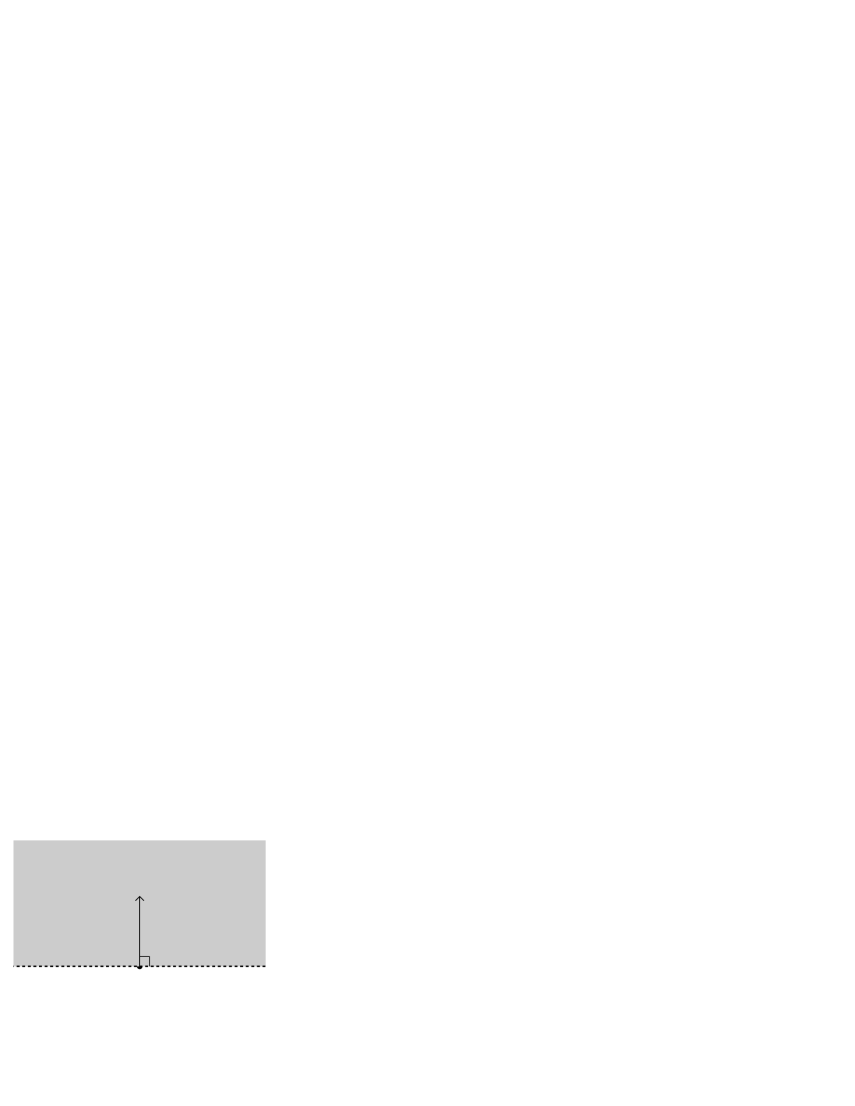
Figure 4: The convergence region for $\theta=0$

Figure 5: The integral path for $\theta=\pi/9$

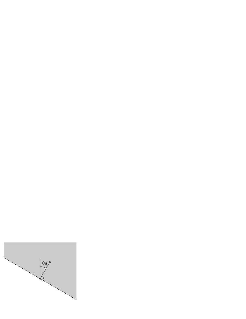
Figure 6: The convergence region for $\theta=\pi/9$

Lemma 8.

If $|\theta-\theta^{\prime}|<\pi/d$, then $\varphi_{\theta}(w)=\varphi_{\theta^{\prime}}(w)$ holds for $w\in e^{-i\theta r}\mathbf{H}\cap e^{-i\theta^{\prime}r}\mathbf{H}$.

Proof.

Put

$$\gamma_{1,R}(t) :=te^{i\theta}\,(0\leq t\leq R), \gamma_{2,R}(t) :=te^{i\theta^{\prime}}\,(0\leq t\leq R), \gamma_{3,R}(\theta^{\prime\prime}) :=Re^{i\theta^{\prime\prime}}\,(\theta\leq\theta^{\prime\prime}\leq\theta^{\prime}).$$

By the Cauchy’s integral formula, we have

$$\int_{\gamma_{1,R}}\Phi dz-\int_{\gamma_{2,R}}\Phi dz+\int_{\gamma_{3,R}}\Phi dz=0.$$ (15)

Here, we put $\Phi=(2\pi)^{-1/2}\exp\left(iwz^{r}-z^{2}/2\right).$ By some calculations, we have that there exist $M>0$ and $\varepsilon>0$ such that

$$\left|\int_{\gamma_{3,R}}\Phi dz\right|\leq MR\exp\left(-\varepsilon R^{r}\right).$$

Taking the limit of (15) as $R$ approaches inifinity, we have $\varphi_{\theta}(z)-\varphi_{\theta^{\prime}}(z)=0.$ ∎

In the second, we disscuss on the analytic continuation of the each term of (3). Let us consider the following integral:

$$\psi(z;\theta,\theta^{\prime},\phi):=\int_{\gamma_{\phi}}e^{-iwz}\left(\varphi_{\theta}(w)-\varphi_{\theta^{\prime}}(w)\right)^{n}dw.$$ (16)

where $\theta,\theta^{\prime},\phi\in\mathbf{R}$, $z\in\mathbf{C}$, and the integral path $\gamma_{\phi}$ is defined by (14).

Lemma 9.

Suppose $\Im(e^{i(\phi+\theta r)})\geq 0$ and $\Im(e^{i(\phi+\theta^{\prime}r)})\geq 0$. Then the integral (16) converges for $z\in-\exp(-i\phi)H$.

Proof.

By the binomial expansion, the integral (16) equals to

$$\sum_{k=0}^{n}\binom{n}{k}(-1)^{n-k}\int_{\gamma_{\phi}}e^{-iwz}\varphi_{\theta}(w)^{k}\varphi_{\theta^{\prime}}(w)^{n-k}dw.$$

With some calculation, the each term of the above expression can be written as

$$\int_{\gamma_{\phi}}e^{-iwz}\varphi_{\theta}(w)^{k}\varphi_{\theta^{\prime}}(w)^{n-k}dw=\frac{1}{(2\pi)^{n/2}}\int_{0}^{\infty}\int_{\mathbf{R}_{>0}^{n}}\exp\left(-h_{1}(z,t)s+h_{2}(t)\right)dtds,$$

where we put $t:=(t_{1},\dots,t_{n})^{\top}$, $dt:=dt_{1}\dots dt_{n}$,

$$h_{1}(z,t) =ie^{i\phi}\left(z-e^{i\theta r}\sum_{\ell=1}^{k}t_{\ell}^{r}-e^{i\theta^{\prime}r}\sum_{\ell=k+1}^{n}t_{\ell}^{r}\right), h_{2}(t) =-\frac{1}{2}\left(e^{2i\theta}\sum_{\ell=1}^{k}t_{\ell}^{2}+e^{2i\theta^{\prime}}\sum_{\ell=k+1}^{n}t_{\ell}^{2}\right).$$

By the Fubini-Tonelli theorem, it is enough to consider the convergence of the following integral:

$$\int_{\mathbf{R}_{>0}^{n}}\int_{0}^{\infty}\left|\exp\left(-h_{1}(z,t)s+h_{2}(t)\right)\right|dsdt.$$ (17)

For $z\in-\exp(-i\phi)H$, we have $\Re(ize^{i\phi})>0$. This inequality and the assumption $\Re(-ie^{i(\phi+\theta r)})\geq 0$ and $\Re(-ie^{i(\phi+\theta^{\prime}r)})\geq 0$ imply $\Re h_{1}(z,t)>0$. Hence, the integral (17) equals to

$$\int_{\mathbf{R}_{>0}^{n}}\left|\exp\left(h_{2}(t)\right)\right|\int_{0}^{\infty}\exp\left(-s\Re h_{1}(z,t)\right)dsdt=\int_{\mathbf{R}_{>0}^{n}}\frac{\left|\exp\left(h_{2}(t)\right)\right|}{\Re h_{1}(z,t)}dt.$$ (18)

By the assumptions, the integral (18) is bounded from above by

$$\frac{1}{\Re(ize^{i\phi})}\int_{\mathbf{R}_{>0}^{n}}\left|\exp\left(h_{2}(t)\right)\right|dt =\frac{1}{\Re(ize^{i\phi})}\left(\int_{0}^{\infty}e^{-\frac{1}{2}\cos(2\theta)t^{2}}dt\right)^{k}\left(\int_{0}^{\infty}e^{-\frac{1}{2}\cos(2\theta^{\prime})t^{2}}dt\right)^{n-k}$$

$$=\frac{1}{\Re(ize^{i\phi})}\left(\frac{\pi}{2\cos(\theta)}\right)^{k/2}\left(\frac{\pi}{2\cos(\theta^{\prime})}\right)^{(n-k)/2}<\infty.$$

Therefore, the integral (16) converges. ∎

Lemma 10.

Suppose $\Im(e^{i(\phi_{k}+\theta r)})\geq 0$ and $\Im(e^{i(\phi_{k}+\theta^{\prime}r)})\geq 0$ for $k=1,2$. The equation

$$\psi(z;\theta,\theta^{\prime},\phi_{1})=\psi(z;\theta,\theta^{\prime},\phi_{2})$$

holds for $z\in\left(-\exp(-i\phi_{1})\right)\cap\left(-\exp(-i\phi_{2})\right)$.

Proof.

Put

$$\gamma_{1,R}(t) :=te^{i\phi_{1}}\,(0\leq t\leq R), \gamma_{2,R}(t) :=te^{i\phi_{2}}\,(0\leq t\leq R), \gamma_{3,R}(\phi) :=Re^{i\phi}\,(\phi_{1}\leq\phi\leq\phi_{2}).$$

By the Cauchy’s integral formula, we have

$$\int_{\gamma_{1,R}}\Phi dw-\int_{\gamma_{2,R}}\Phi dw+\int_{\gamma_{3,R}}\Phi dw=0,$$ (19)

where we put $\Phi=e^{-iwz}\left(\varphi_{\theta}(w)-\varphi_{\theta^{\prime}}(w)\right)^{n}.$ By some calculations, we have

$$\left|\int_{\gamma_{3,R}}\Phi dw\right|\leq MR\exp\left(-R\right)$$

for sufficiently large $M>0$. Taking the limit of (19) as $R$ approaches inifinity, we have $\psi(z;\theta,\theta^{\prime},\phi_{1})-\psi(z;\theta,\theta^{\prime},\phi_{2})=0.$ ∎

Theorem 3.

Let $\varepsilon>0$ be a sufficiently small positive number and $x$ be a continuous point of $f_{X}$. When $r$ is odd, we have

$$f_{X}(x)=\begin{cases}\psi(x;\varepsilon,\pi,-\varepsilon r)-\psi(x;-\varepsilon,\pi,\pi+\varepsilon r)&(x>0),\\ \psi(x;0,\pi-\varepsilon,\varepsilon r)-\psi(x;0,\pi+\varepsilon,\pi-\varepsilon r)&(x<0).\end{cases}$$

When $r$ is even, we have

$$f_{X}(x)=\begin{cases}\psi(x;\varepsilon,\pi+\varepsilon,-\varepsilon r)-\psi(x;-\varepsilon,\pi-\varepsilon,\pi+\varepsilon r)&(x>0),\\ \psi(x;0,\pi,\varepsilon r)-\psi(x;0,\pi,\pi-\varepsilon r)&(x<0).\end{cases}$$

Proof.

When $r$ is odd and $x>0$, we have

$$f_{X}(x) =\frac{1}{2\pi}\lim_{y\rightarrow+0}\left(\psi(x-iy;0,\pi,0)-\psi(x+iy;0,\pi,\pi)\right)$$

$$=\frac{1}{2\pi}\lim_{y\rightarrow+0}\left(\psi(x-iy;\varepsilon,\pi,0)-\psi(x+iy;0,\pi+\varepsilon,\pi)\right)$$

$$=\frac{1}{2\pi}\lim_{y\rightarrow+0}\left(\psi(x-iy;\varepsilon,\pi,-\varepsilon r)-\psi(x+iy;0,\pi+\varepsilon,\pi+\varepsilon r)\right)$$

$$=\frac{1}{2\pi}\left(\psi(x;\varepsilon,\pi,-\varepsilon r)-\psi(x;0,\pi+\varepsilon,\pi+\varepsilon r)\right)$$

When $r$ is odd and $x<0$, we have

$$f_{X}(x) =\frac{1}{2\pi}\lim_{y\rightarrow+0}\left(\psi(x-iy;0,\pi,0)-\psi(x+iy;0,\pi,\pi)\right)$$

$$=\frac{1}{2\pi}\lim_{y\rightarrow+0}\left(\psi(x-iy;-\varepsilon,\pi,0)-\psi(x+iy;0,\pi-\varepsilon,\pi)\right)$$

$$=\frac{1}{2\pi}\lim_{y\rightarrow+0}\left(\psi(x-iy;-\varepsilon,\pi,\varepsilon r)-\psi(x+iy;0,\pi-\varepsilon,\pi-\varepsilon r)\right)$$

$$=\frac{1}{2\pi}\left(\psi(x;-\varepsilon,\pi,\varepsilon r)-\psi(x;0,\pi-\varepsilon,\pi-\varepsilon r)\right)$$

When $r$ is even and $x>0$, we have

$$f_{X}(x) =\frac{1}{2\pi}\lim_{y\rightarrow+0}\left(\psi(x-iy;0,\pi,0)-\psi(x+iy;0,\pi,\pi)\right)$$

$$=\frac{1}{2\pi}\lim_{y\rightarrow+0}\left(\psi(x-iy;\varepsilon,\pi+\varepsilon,0)-\psi(x+iy;0,\pi+\varepsilon,\pi)\right)$$

$$=\frac{1}{2\pi}\lim_{y\rightarrow+0}\left(\psi(x-iy;\varepsilon,\pi+\varepsilon,-\varepsilon r)-\psi(x+iy;0,\pi+\varepsilon,\pi+\varepsilon r)\right)$$

$$=\frac{1}{2\pi}\left(\psi(x;\varepsilon,\pi+\varepsilon,-\varepsilon r)-\psi(x;0,\pi+\varepsilon,\pi+\varepsilon r)\right)$$

When $r$ is odd and $x<0$, we have

$$f_{X}(x) =\frac{1}{2\pi}\lim_{y\rightarrow+0}\left(\psi(x-iy;0,\pi,0)-\psi(x+iy;0,\pi,\pi)\right)$$

$$=\frac{1}{2\pi}\lim_{y\rightarrow+0}\left(\psi(x-iy;-\varepsilon,\pi,0)-\psi(x+iy;0,\pi-\varepsilon,\pi)\right)$$

$$=\frac{1}{2\pi}\lim_{y\rightarrow+0}\left(\psi(x-iy;-\varepsilon,\pi,\varepsilon r)-\psi(x+iy;0,\pi-\varepsilon,\pi-\varepsilon r)\right)$$

$$=\frac{1}{2\pi}\left(\psi(x;-\varepsilon,\pi,\varepsilon r)-\psi(x;0,\pi-\varepsilon,\pi-\varepsilon r)\right)$$

∎

Remark 1.

The all of integral representations in Theorem 3 make sense as Lebesgue integral. As we have shown in Lemma 9, when we write the integral in Theorem 3 into an integral on $\mathbf{R}$, the integrand is a Lebesgue integrable function.

Acknowledgements: We are grateful to K. Yajima, T. Oshima, and S.-J. Matsubara-Heo for valuable comments to Proposition 1. This work was supported by MEXT/JSPS KAKENHI Grand Numbers JP 25220001, 18J01507.

References

[1]
A. Castaño-Martínez and F. López-Blázquez.
Distribution of a sum of weighted noncentral chi-square variables.
TEST, 14(2):397–415, December 2005.
[2]
U. Graf.
Introduction to Hyperfunctions and Their Integral Transforms.
Birkhäuser, Basel, 2010.
[3]
T. Hibi.
Gröbner Bases: Statistics and Software System.
Springer Japan, Tokyo, 2014.
[5]
A. Kaneko.
Introduction to Hyperfunctions.
KTK Scientific Publishers, Tokyo, 1988.
[6]
T. Kawai.
On the theory of fourier hyperfunctions and its applications to
partial differential equations with constant coefficients.
Journal of the Faculty of Science, the University of Tokyo,
17(3):467–517, December 1970.
[7]
T. Koyama and A. Takemura.
Holonomic gradient method for distribution function of a weighted sum
of noncentral chi-square random variables.
Computational Statistics, 31(4):1645–1659, December 2016.
[8]
N. Marumo, T. Oaku, and A. Takemura.
Properties of powers of functions satisfying second-order linear
differential equations with applications to statistics.
Japan Journal of Industrial and Applied Mathematics,
32:553–572, July 2015.
[9]
H. Nakayama, K. Nishiyama, M. Noro, K. Ohara, T. Sei, N. Takayama, and
A. Takemura.
Holonomic gradient descent and its application to the
Fisher-Bingham integral.
Advances in Applied Mathematics, 47:639–658, 2011.
[10]
H. Ogata and H. Hirayama.
Hyperfunction method for numerical integrations.
Transactions of the Japan Society for Industrial and Applied
Mathematics, 26(1):33–43, 2016.
(in Japanese).
[11]
M. Sato.
Theory of hyperfunctions.
Sûgaku, 10:1–27, 1958.
in Japanese.
[12]
David Williams.
Probability with Martingales.
Cambridge University Press, Cambridge, 1991.