Geometric properties of a binary non-Pisot inflation
and absence of absolutely continuous diffraction

Abstract.

One of the simplest non-Pisot substitution rules is investigated in its geometric version as a tiling with intervals of natural length as prototiles. Via a detailed renormalisation analysis of the pair correlation functions, we show that the diffraction measure cannot comprise any absolutely continuous component. This implies that the diffraction, apart from a trivial Bragg peak at the origin, is purely singular continuous. En route, we derive various geometric and algebraic properties of the underlying Delone dynamical system, which we expect to be relevant in other such systems as well.

1. Introduction

The spectral structure of substitution dynamical systems is well studied, and many results are known; see [31] for a systematic introduction. The theory is in good shape for substitutions of constant length, both in one and in higher dimensions; see [19, 33, 21, 4, 11] as well as [3] and references therein. This is due to the fact that, for these systems, the symbolic side and the geometric realisation with tiles of natural size coincide, which also leads to a rather direct relation between the diffraction measures of the system (and its factors) on the one hand and the spectral measures on the other; see [8] and references therein.

In general, the spectral theory of a substitution system and that of its geometric counterpart can differ considerably [16], in particular when the inflation multiplier fails to be a Pisot-Vijayaraghavan (PV) number [3, Def. 2.13]. In fact, beyond the substitutions of constant length, it often is simpler and ultimately more revealing to use the geometric setting with natural tile (or interval) sizes, as suggested by Perron–Frobenius theory. We adopt this point of view below, and then speak of inflation rules to make the distinction. Our entire analysis in this paper will be in one dimension, where the tiles are just intervals.

Since rather little is known when one leaves the realm of PV inflation multipliers, we present a detailed analysis of one of the simplest non-Pisot (or non-PV) inflation rules on two letters, for which we finally establish that the diffraction spectrum of the corresponding Delone sets on the real line, apart from the trivial peak at $0$, is purely singular continuous. En route, we shall encounter a number of concepts and results that are described in some detail, in a way that will facilitate generalisations to other inflation rules (and possibly also to higher dimensions) in the future. A key ingredient to our analysis is the study of the pair correlation functions via their exact renormalisation relations. The latter are analogous to those recently derived [2] for the Fibonacci inflation, where they led to a spectral purity result and then to pure point spectrum. This re-proved a known result in an independent way.

In the binary non-Pisot system studied below, the situation is more complex because the spectrum is mixed, whence it remains to determine the nature of the continuous part. To the best of our knowledge, the answer is not in the literature, though the absence of absolutely continuous components is certainly expected [21, 4, 2, 12]. In anticipation of future work, we do not present the shortest path to the result, as that would mean to restrict more than necessary to methods that are limited to binary alphabets and to this particular example. Instead, we use the concrete system to investigate various concepts from [2] in this more complex case, with an eye to possible extensions and generalisations.

The paper is organised as follows. In Section 2, we introduce the binary system via its symbolic substitution rule and the matching geometric inflation tiling of the real line by two types of intervals, following the general notions and results from [3]. Such a tiling is simultaneously considered as a two-component Delone set, by taking the left endpoints of the intervals as reference points. We also recall the construction of the hull and its dynamical system, together with the key properties of the latter. Section 3 introduces the pair correlation functions and derives exact renormalisation relations, which are then studied for their general solutions. This part is not strictly needed for our later analysis, but is interesting in its own right and helps to understand the differences to the cases treated in [2].

To continue, we need a reformulation of the pair correlation functions in terms of translation bounded measures and their Fourier transforms, which is provided in Section 4. This step emphasises the importance of two specific matrix families, whose structure will later provide some arguments needed in the exclusion of absolutely continuous diffraction. Section 5 analyses several properties of these matrix families by means of the (complex resp. real) algebras generated by them. Once again, some of these results go beyond what we need for our final goal, but highlight the algebraic structure of the problem.

Section 6 returns to the correlation measures and their Fourier transforms. After splitting the transformed pair correlation measures into their spectral parts (Lebesgue decomposition), we rule out the existence of an absolutely continuous component by a suitable iterated application of the renormalisation relations in two directions. This approach employs the determination of the corresponding extremal Lyapunov exponents, some details of which are given in Appendix A. Two underlying renormalisation arguments are further explained in Appendix B, in the simpler setting of a scalar equation. Section 7 covers an application to the diffraction in the balanced weight case, where the pure point part is extinct. In particular, we illustrate one specific case of a singular continuous measure in this setting, based on a precise numerical calculation of the corresponding (continuous) distribution function.

2. Setting and preliminaries

2.1. Substitution, inflation and hull

We consider the primitive two-letter substitution

(2.1) $$\varrho\!:\quad\begin{array}[]{l}0\mapsto 0111\\ 1\mapsto 0\end{array}$$

on the alphabet $\{0,1\}$. It defines a unique (symbolic) hull $\mathbb{X}$, for instance via the shift orbit closure of the bi-infinite fixed point $w$ of $\varrho^{2}$ with legal seed $w^{(0)}=0|0$,

$$0|0\,\stackrel{{\scriptstyle\varrho^{2}}}{{\longmapsto}}\,w^{(1)}=0111000|0111000\,\stackrel{{\scriptstyle\varrho^{2}}}{{\longmapsto}}\,\dots\,\stackrel{{\scriptstyle\varrho^{2}}}{{\longmapsto}}\,w^{(i)}\;\xrightarrow{\;i\to\infty\;}\;w=\varrho^{2}(w)\hskip 0.5pt,$$

where finite words are considered as embedded into $\{0,1\}^{\mathbb{Z}{\hskip 0.5pt}}$ and $|$ marks the reference point (between position $-1$ and $0$). In particular, $(\mathbb{X},\mathbb{Z}{\hskip 0.5pt})$ with the continuous $\mathbb{Z}{\hskip 0.5pt}$-action generated by the shift is a minimal topological dynamical system. There is precisely one shift invariant probability measure $\mu_{\mathbb{X}}$ on $\mathbb{X}$, namely the patch (or word) frequency measure, so that $(\mathbb{X},\mathbb{Z}{\hskip 0.5pt},\mu_{\mathbb{X}})$ is strictly ergodic. The invariant measure is intimately connected with the substitution origin; see [31, 35, 3] for background.

The corresponding integer substitution matrix is

(2.2) $$M\;=\;\begin{pmatrix}1&1\\ 3&0\end{pmatrix},$$

with irreducible characteristic polynomial $\det(M-x\mathbbm{1})=x^{2}-x-3$ and Perron–Frobenius (PF) eigenvalue $\lambda=(1+\sqrt{13}\,)/2\approx 2.302\hskip 0.5pt776$. Its algebraic conjugate, which is also the second eigenvalue of $M$, is $\lambda^{\prime}=(1-\sqrt{13}\,)/2=1-\lambda\approx-1.302\hskip 0.5pt776$, which lies outside the unit circle, wherefore $\lambda$ is not a PV number. Since $\lvert\det(M)\rvert=3$ is prime, $M$ has no root in $\mathrm{Mat}(2,\mathbb{Z}{\hskip 0.5pt})$, hence $\varrho$ cannot have a substitutional root.

The statistically normalised right eigenvector $v_{\text{PF}}$ to the eigenvalue $\lambda$ is

(2.3) $$v_{\text{PF}}\;=\;(\nu_{0},\nu_{1})^{t}\;=\;\bigl{(}\lambda^{-1},3\lambda^{-2}\bigr{)}^{t}\;=\;\frac{\raisebox{-2.0pt}{$1$}}{\raisebox{0.5pt}{$3$}}\,\bigl{(}\lambda-1,4-\lambda\bigr{)}^{t}\;\approx\;\bigl{(}0.434,0.566\bigr{)}^{t},$$

which determines the (relative) frequencies of the two letters, $\nu_{0}$ and $\nu_{1}$. For a consistent geometric realisation as an inflation rule on two intervals, we use interval lengths according to the left PF eigenvector of $M$, which we choose as $(\lambda,1)$; see Figure 1 for an illustration. Note that this choice is particularly simple from an algebraic point of view, as the two lengths are the generating elements of $\mathbb{Z}{\hskip 0.5pt}[\lambda]$. From a dynamical perspective, it would perhaps be more natural to make a choice with average length $1$, but this would give a more complicated algebraic structure for the coordinates.

Figure 1. Inflation rule for the substitution $\varrho$ of Eq. (2.1). It consists of two steps, an expansion of the intervals by $\lambda$ and the ensuing subdivision into intervals of the original length in the correct order.

Now, let $\varLambda^{w}$ denote the point set of left interval end points that corresponds to our above fixed point $w$, so

(2.4) $$\varLambda^{w}\;=\;\bigl{\{}\ldots,-1\!-\!3\lambda,-3\lambda,-2\lambda,-\lambda,0,\lambda,1\!+\!\lambda,2\!+\!\lambda,3\!+\!\lambda,3\!+\!2\lambda,\ldots\bigr{\}}\;\subset\;\mathbb{Z}{\hskip 0.5pt}[\lambda]\,.$$

This is a Delone set of density $\operatorname{\mathrm{dens}}(\varLambda^{w})=(6+\lambda)/13\approx 0.638{\hskip 0.5pt}675$, and its orbit closure under the natural translation action of $\mathbb{R}\hskip 0.5pt$ defines the geometric hull

(2.5) $$\mathbb{Y}\,:=\,\overline{\{t+\varLambda_{\phantom{\hat{\hat{I}}}}^{w}:t\in\mathbb{R}\hskip 0.5pt\}}^{\mathrm{\hskip 0.5ptLT}}\hskip 0.5pt,$$

where the closure is taken in the local topology; see [3] for details. Note that $\mathbb{Y}$ is compact in the local topology, as a result of $\varLambda^{w}$ being a Delone set of finite local complexity, which means that the Minkowski difference $\varLambda^{w}-\varLambda^{w}$ is a locally finite set.

Now, $(\mathbb{Y},\mathbb{R}\hskip 0.5pt)$ is once again a minimal topological dynamical system, which still only has one invariant probability measure, namely the one induced by $\mu_{\mathbb{X}}$ from above, so that $(\mathbb{Y},\mathbb{R}\hskip 0.5pt,\mu_{\mathbb{Y}})$ is strictly ergodic, too. This system can be obtained as a suspension of the previous one, with a non-constant roof function; see [18, Ch. 11] for background. It is this latter system that we investigate now in more detail. To this end, we also need the Minkowski difference

$$\varDelta\,:=\,\varLambda^{w}-\varLambda^{w}\,=\,\bigl{\{}0,\pm 1,\pm 2,\pm\lambda,\pm 3,\pm(1\!+\!\lambda),\pm(2\!+\!\lambda),\pm 2\lambda,\pm(3\!+\!\lambda),\pm(1\!+\!2\lambda),\ldots\bigr{\}},$$

which is the set of distances between points in $\varLambda^{w}$ and satisfies $\varDelta\subset\mathbb{Z}{\hskip 0.5pt}[\lambda]$.

Proposition 2.1.

Let $\mathbb{Y}$ be the geometric hull from Eq. (2.5), and $\varLambda\in\mathbb{Y}$. Then, the Minkowski difference $\varDelta_{\varLambda}:=\varLambda-\varLambda$ is a locally finite subset of $\mathbb{R}\hskip 0.5pt$, but it is not uniformly discrete. One has $\varDelta_{\varLambda}=\varDelta$ for all $\varLambda\in\mathbb{Y}$, so the difference set is constant on $\mathbb{Y}$.

Proof.

The hull $\mathbb{Y}$ is the translation orbit closure of the Delone set $\varLambda^{w}$ from Eq. (2.4). Since $\lambda\varLambda^{w}\subset\varLambda^{w}$ by construction, but $\lambda$ is not a PV number, the set $\varLambda^{w}$ cannot be a Meyer set; compare [3, Thm. 2.4]. Consequently, $\varLambda^{w}-\varLambda^{w}$ is discrete, but not uniformly discrete. Since the difference set is also closed, it is locally finite.

The inflation rule derived from $\varrho$ is primitive, whence we know form standard arguments (compare [3, Ch. 4] for details) that the hull $\mathbb{Y}$ consists of the LI class of $\varLambda^{w}$, which means that any two elements of $\mathbb{Y}$ are locally indistinguishable. This implies that $\varDelta_{\varLambda}$ with $\varLambda\in\mathbb{Y}$ cannot depend on $\varLambda$, which establishes the second claim. ∎

In what follows, we will freely move between the tiling picture and its representation as a Delone set, where we tacitly make use of the equivalence concept of mutual local derivability (MLD); compare [3, Sec. 5.2] and references therein for background.

2.2. Natural autocorrelation and diffraction

Next, let us recall the notion of the natural autocorrelation of $\varLambda\in\mathbb{Y}$, compare [25] or [3, Def. 9.1], which is usually done by first turning $\varLambda$ into the Dirac comb $\delta_{\!\varLambda}:=\sum_{x\in\varLambda}\delta_{x}$. The latter is both a tempered distribution and a translation bounded measure on $\mathbb{R}\hskip 0.5pt$. In particular, $\delta_{\!\varLambda}$ is not a finite measure. Its autocorrelation $\gamma$ is then defined as the volume-averaged (or Eberlein) convolution

$$\gamma\,=\,\delta_{\!\varLambda}\circledast\delta_{-\varLambda}\,:=\lim_{n\to\infty}\frac{\delta_{\!\varLambda_{r}}\!*\delta_{-\varLambda_{r}}}{2\hskip 0.5ptr}$$

where $\varLambda_{r}=\varLambda\cap[-r,r]$. The existence of the limit, for any $\varLambda\in\mathbb{Y}$, is a consequence of unique ergodicity. Once again, $\gamma$ is not a finite measure, but it is translation bounded. In fact, from a simple calculation together with Proposition 2.1, one can see that $\gamma=\sum_{z\in\varDelta}\eta(z)\hskip 0.5pt\delta_{z}$ with the autocorrelation coefficients

$$\eta(z)\,=\lim_{r\to\infty}\frac{\operatorname{\mathrm{card}}\bigl{(}\varLambda_{r}\cap(z+\varLambda_{r})\bigr{)}}{2\hskip 0.5ptr}\,=\lim_{r\to\infty}\frac{\operatorname{\mathrm{card}}\bigl{(}\varLambda_{r}\cap(z+\varLambda)\bigr{)}}{2\hskip 0.5ptr}.$$

More generally, we also need to consider weighted Dirac combs $\omega$ with (generally complex) weights $u_{0}$ and $u_{1}$ for the two letters (or point types). They are defined as

(2.6) $$\omega\,=\,\omega_{\!\varLambda,u}\,=\sum_{x\in\varLambda}u(x)\,\delta_{x}$$

with $u(x)\in\{u_{0},u_{1}\}$ depending on whether $x$ is the left endpoint of an interval of type $0$ or $1$. In other words, we consider $\varLambda=\varLambda^{(0)}\hskip 0.5pt\dot{\cup}\varLambda^{(1)}$ as the disjoint union of two Delone sets, according to the two types of points in $\varLambda$, and hence as a two-component Delone set. In our case at hand, the two versions are MLD, because the prototiles (intervals) have different lengths. Note that, for $i\in\{0,1\}$, we then have the density relations

(2.7) $$\operatorname{\mathrm{dens}}\bigl{(}\varLambda^{(i)}\bigr{)}\,=\,\nu_{i}\,\operatorname{\mathrm{dens}}(\varLambda)$$

with the frequencies $\nu_{i}$ from Eq. (2.3).

The natural autocorrelation of such a Dirac comb $\omega$ is

(2.8) $$\gamma_{u}\,=\,\omega\circledast\widetilde{\omega}\,:=\lim_{r\to\infty}\frac{\omega_{r}*\widetilde{\omega_{r}}}{2\hskip 0.5ptr}\hskip 0.5pt,$$

with $\omega=\omega_{\!\varLambda,u}$ and $\omega_{r}$ denoting the restriction of $\omega$ to the interval $[-r,r]$. Moreover, the twisted measure $\widetilde{\mu}$ is defined by $\widetilde{\mu}(g)=\overline{\mu(\widetilde{g})}$ for test functions $g\in C_{\mathsf{c}}(\mathbb{R}\hskip 0.5pt)$, with $\widetilde{g}(x):=\overline{g(-x)}$; see [3, Ch. 9.1] for background. As before, the existence of the limit is a consequence of unique ergodicity, and we have $\gamma_{u}=\sum_{z\in\varDelta}\eta_{u}(z)\hskip 0.5pt\delta_{z}$, this time with

(2.9) $$\eta_{u}(z)\;=\,\lim_{r\to\infty}\,\frac{\raisebox{-2.0pt}{$1$}}{\raisebox{0.5pt}{$2\hskip 0.5ptr$}}\!\sum_{y,y+z\in\varLambda_{r}}\!\!\overline{u(y)}\,u(y+z)\hskip 0.5pt.$$

By construction, any such autocorrelation $\gamma_{u}$ is a positive definite measure, which means that $\gamma_{u}(g*\widetilde{g})\geqslant 0$ holds for all $g\in C_{\mathsf{c}}(\mathbb{R}\hskip 0.5pt)$. This is significant because any positive definite measure is Fourier transformable as a measure, which is a non-trivial statement since $\gamma_{u}$ is not a finite measure. Its Fourier transform is then a positive measure, as a consequence of the Bochner–Schwartz theorem; see [13, 32] for background.

Proposition 2.2.

Given arbitrary weights $u_{0},u_{1}\in\mathbb{C}\hskip 0.5pt$ for the two types of points, the autocorrelation measure $\gamma_{u}$ is positive definite, and it is the same for all $\varLambda\in\mathbb{Y}$, which means that $\gamma_{u}$ is the autocorrelation both for an arbitrary element of the hull and for the entire hull. The analogous statement holds for the diffraction measure $\widehat{\gamma_{u}}$, which is always a translation bounded, positive measure.

Proof.

As explained above, the first claim is a consequence of Eq. (2.8), because positive definiteness of measures is preserved under limits in the vague topology.

The second claim on the autocorrelation follows from the uniform existence of patch frequencies together with the fact that any two elements of the hull are locally indistinguishable.

The statement on the diffraction then is a consequence of the uniqueness of the Fourier transform. The positivity of $\widehat{\gamma_{u}}$ is clear by Bochner–Schwartz, while its translation boundedness follows from [13, Prop. 4.9]. ∎

The Fourier transform $\widehat{\gamma_{u}}$ is called the diffraction measure of $\omega$, which is thus always a positive measure. With respect to Lebesgue measure on $\mathbb{R}\hskip 0.5pt$, it has the unique decomposition

$$\widehat{\gamma_{u}}\;=\;\bigl{(}\widehat{\gamma_{u}}\bigr{)}_{\mathsf{pp}}+\bigl{(}\widehat{\gamma_{u}}\bigr{)}_{\mathsf{sc}}+\bigl{(}\widehat{\gamma_{u}}\bigr{)}_{\mathsf{ac}}$$

into its pure point, singular continuous and absolutely continuous parts; see [3, Rem. 9.3] for more. Our aim is to determine the precise nature of $\widehat{\gamma}$ for our system.

Because we are dealing with a non-PV inflation multiplier $\lambda$, we get the following result on the pure point part of the diffraction measure.

Theorem 2.3.

Let $\varLambda=\varLambda^{(0)}\hskip 0.5pt\dot{\cup}\varLambda^{(1)}$ be a fixed element of the hull $\mathbb{Y}$. Consider the weighted Dirac comb $\omega_{\!\varLambda,u}=u_{0}\,\delta_{\!\!\varLambda_{\vphantom{a}}^{(0)}}+u_{1}\,\delta_{\!\!\varLambda_{\vphantom{a}}^{(1)}}$, with arbitrary complex weights $u_{0}$ and $u_{1}$. Then, the pure point part of the corresponding diffraction measure $\widehat{\gamma_{\!\varLambda,u}}$ is given by

$$\bigl{(}\widehat{\gamma_{u}}\bigr{)}_{\mathsf{pp}}\;=\;I_{0}\,\delta_{0}\,,\quad\text{with }\,I_{0}\,=\,\big{\lvert}\operatorname{\mathrm{dens}}(\varLambda^{w})\,(u\cdot v_{\mathrm{PF}})\big{\rvert}^{2}\,=\,\big{\lvert}\tfrac{2\lambda-1}{13}u_{0}+\tfrac{7-\lambda}{13}u_{1}\big{\rvert}^{2}.$$

In particular, the pure point part is the same for all $\varLambda\in\mathbb{Y}$.

Proof.

The claim is trivial for $u_{0}=u_{1}=0$, so let us assume that at least one of the weights is nonzero. Then, the dynamical system $(\mathbb{Y}_{u},\mathbb{R}\hskip 0.5pt)$, as obtained by the vague closure of the set $\{\delta_{t}*\omega_{\!\varLambda,u}:t\in\mathbb{R}\hskip 0.5pt\}$, is seen to be topologically conjugate to $(\mathbb{Y},\mathbb{R}\hskip 0.5pt)$ via standard MLD arguments. We thus know from [35, Thm. 4.3 and Cor. 4.5] that we only have the trivial eigenfunction for $(\mathbb{Y}_{u},\mathbb{R}\hskip 0.5pt)$.

Now, assume $\widehat{\gamma_{u}}\bigl{(}\{k\}\bigr{)}=I(k)\neq 0$ for some $k\neq 0$. We then know from [25, Thm. 3.4] and [28, Thm. 5] that $I(k)=\big{\lvert}a_{\varLambda,u}(k)\big{\rvert}^{2}$, with the Fourier–Bohr coefficient

$$a_{\varLambda,u}(k)\,=\lim_{r\to\infty}\frac{\raisebox{-2.0pt}{$1$}}{\raisebox{0.5pt}{$2\hskip 0.5ptr$}}\sum_{x\in\varLambda_{r}}u(x)\,\,\mathrm{e}^{-2\pi\hskip 0.5pt\mathrm{i}kx}$$

and $u(x)$ as in Eq. (2.6). Note that this coefficient exists for all $\varLambda\in\mathbb{Y}$ (and even uniformly so) for our system due to unique ergodicity. Note also that the coefficient depends on $\varLambda$, while $I(k)$ does not. In fact, for fixed $u$, the map given by $\varLambda\mapsto a_{\varLambda,u}(k)$ defines an eigenfunction (in fact, a continuous one) of $(\mathbb{Y}_{u},\mathbb{R}\hskip 0.5pt)$ because $a_{t+\varLambda,u}(k)=\,\mathrm{e}^{-2\pi\hskip 0.5pt\mathrm{i}kt}a_{\varLambda,u}(k)$ for $t\in\mathbb{R}\hskip 0.5pt$; compare [25, 28]. Since we know that such an eigenfunction cannot exist, we must have $I(k)=0$.

Finally, the formula for $I_{0}$ follows from an application of [3, Prop. 9.2] by observing that, for a weighted Dirac comb supported on $\varLambda$, the averaging formula stated there reduces to the absolute square of the volume-averaged weights, via Eq. (2.7). ∎

In other words, we can only have the trivial central Bragg peak. Later, we will be interested in the situation that $I_{0}=0$, which we refer to as the balanced weight case. Since no recursive formula for the coefficients $\eta(z)$ is known, and since it is desirable to have a systematic approach to $\gamma$ for arbitrary choices of the weights, we now turn to the pair correlation functions and their properties. This will produce another path to $\eta$ and $\gamma$.

3. Renormalisation approach to pair correlation functions

As before, we use the tiling picture (with the two types of intervals as prototiles) and the two-component Delone set picture in parallel. These two versions obviously give topologically conjugate dynamical systems, wherefore we simply identify them canonically. Which representation we use will always be clear from the context.

3.1. Pair correlation functions

Let $\varLambda$ be any element of the (geometric) hull $\mathbb{Y}$, and let $\nu_{ij}(z)$ denote the relative frequency of distance $z$ from a left endpoint of an interval of type $i$ to one of type $j$, with $i,j\in\{0,1\}$. Decomposing $\varLambda=\varLambda^{(0)}\hskip 0.5pt\dot{\cup}\varLambda^{(1)}$ as before, this means

(3.1) $$\nu_{ij}(z)\;=\;\lim_{r\to\infty}\frac{\operatorname{\mathrm{card}}\bigl{(}\varLambda^{(i)}_{r}\cap(\varLambda^{(j)}_{r}-z)\bigr{)}}{\operatorname{\mathrm{card}}(\varLambda_{r})}\;=\;\frac{\raisebox{-2.0pt}{$1$}}{\raisebox{0.5pt}{$\operatorname{\mathrm{dens}}(\varLambda)$}}\,\lim_{r\to\infty}\frac{\operatorname{\mathrm{card}}\bigl{(}\varLambda^{(i)}_{r}\cap(\varLambda^{(j)}_{r}-z)\bigr{)}}{2\hskip 0.5ptr}\hskip 0.5pt.$$

These limits exist for any $z\in\mathbb{R}\hskip 0.5pt$, and one has $\nu_{ij}(z)\geqslant 0$. The use of relative frequencies is advantageous because they are dimensionless and thus simplify various statements below.

The four functions $\nu_{ij}$, which we call the pair correlation functions, are well-defined, as another consequence of the unique ergodicity of our system. Clearly, for any $i,j\in\{0,1\}$ and any $z\in\mathbb{R}\hskip 0.5pt$, they satisfy the symmetry relations

(3.2) $$\nu_{ij}(z)\,=\,\nu_{ji}(-z)\hskip 0.5pt.$$

Moreover, we have $\nu_{ij}(z)=0$ for any $z\not\in\varLambda-\varLambda$. To improve on this, for any $\varLambda\in\mathbb{Y}$, decompose $\varLambda=\varLambda^{(0)}\hskip 0.5pt\dot{\cup}\varLambda^{(1)}$ as above and define the point sets

(3.3) $$S_{ij}\,:=\,\varLambda^{(j)}-\varLambda^{(i)}.$$

By an obvious variant of Propositions 2.1 and 2.2, it is clear that each $S_{ij}$ is again independent of the choice of $\varLambda$, hence constant on the hull. Due to strict ergodicity, we then have the following stronger property.

Fact 3.1.

The pair correlation functions $\nu_{ij}$ defined in Eq. (3.1) are independent of the choice of $\varLambda\in\mathbb{Y}$. They satisfy the symmetry relations of Eq. (3.2). Moreover, one has $\nu_{ij}(z)>0$ if and only if $z\in S_{ij}$, where $S_{ij}$ is the set from Eq. (3.3), which is the same for all $\varLambda\in\mathbb{Y}$. ∎

The autocorrelation coefficients $\eta_{u}(z)$ from Eq. (2.9) for the weighted Dirac comb $\omega$ of Eq. (2.6) can now be expressed in terms of the pair correlation functions of $\mathbb{Y}$ as a quadratic form, namely as

(3.4) $$\eta_{u}(z)\;=\;\mathrm{dens}(\varLambda)\!\!\sum_{i,j\in\{0,1\}}\!\!\overline{u_{i}}\;\nu_{ij}(z)\,u_{j}\hskip 0.5pt.$$

This shows that the ‘natural’ objects to study are indeed the pair correlation functions, as their knowledge gives access to the autocorrelation measures (and hence to their Fourier transforms) for any choice of the weights. Also, as mentioned earlier, we are not aware of a functional relation that would determine the coefficients $\eta_{u}(z)$ directly. However, such a relation can be derived from the inflation structure for the four pair correlation functions $\nu_{ij}(z)$; see [2] for related examples.

Proposition 3.2.

The pair correlation functions $\nu_{ij}$ of the hull $\mathbb{Y}$ satisfy the following linear renormalisation equations,

$$\nu_{00}(z) \,=\,\frac{\raisebox{-2.0pt}{$1$}}{\raisebox{0.5pt}{$\lambda$}}\,\Bigl{(}\nu_{00}\bigl{(}\tfrac{z}{\lambda}\bigr{)}+\nu_{01}\bigl{(}\tfrac{z}{\lambda}\bigr{)}+\nu_{10}\bigl{(}\tfrac{z}{\lambda}\bigr{)}+\nu_{11}\bigl{(}\tfrac{z}{\lambda}\bigr{)}\Bigr{)},$$

$$\nu_{01}(z) \,=\,\frac{\raisebox{-2.0pt}{$1$}}{\raisebox{0.5pt}{$\lambda$}}\,\Bigl{(}\nu_{00}\bigl{(}\tfrac{z-\lambda}{\lambda}\bigr{)}+\nu_{00}\bigl{(}\tfrac{z-1-\lambda}{\lambda}\bigr{)}+\nu_{00}\bigl{(}\tfrac{z-2-\lambda}{\lambda}\bigr{)}+\nu_{10}\bigl{(}\tfrac{z-\lambda}{\lambda}\bigr{)}+\nu_{10}\bigl{(}\tfrac{z-1-\lambda}{\lambda}\bigr{)}+\nu_{10}\bigl{(}\tfrac{z-2-\lambda}{\lambda}\bigr{)}\Bigr{)},$$

$$\nu_{10}(z) \,=\,\frac{\raisebox{-2.0pt}{$1$}}{\raisebox{0.5pt}{$\lambda$}}\,\Bigl{(}\nu_{00}\bigl{(}\tfrac{z+\lambda}{\lambda}\bigr{)}+\nu_{00}\bigl{(}\tfrac{z+1+\lambda}{\lambda}\bigr{)}+\nu_{00}\bigl{(}\tfrac{z+2+\lambda}{\lambda}\bigr{)}+\nu_{01}\bigl{(}\tfrac{z+\lambda}{\lambda}\bigr{)}+\nu_{01}\bigl{(}\tfrac{z+1+\lambda}{\lambda}\bigr{)}+\nu_{01}\bigl{(}\tfrac{z+2+\lambda}{\lambda}\bigr{)}\Bigr{)},$$

$$\nu_{11}(z) \,=\,\frac{\raisebox{-2.0pt}{$1$}}{\raisebox{0.5pt}{$\lambda$}}\,\Bigl{(}3\,\nu_{00}\bigl{(}\tfrac{z}{\lambda}\bigr{)}+2\,\nu_{00}\bigl{(}\tfrac{z+1}{\lambda}\bigr{)}+2\,\nu_{00}\bigl{(}\tfrac{z-1}{\lambda}\bigr{)}+\nu_{00}\bigl{(}\tfrac{z+2}{\lambda}\bigr{)}+\nu_{00}\bigl{(}\tfrac{z-2}{\lambda}\bigr{)}\Bigr{)},$$

together with $\nu_{ij}(z)=0$ for any $z\not\in S_{ij}$ and the symmetry relations $\nu_{ji}(z)=\nu_{ij}(-z)$ for all $z\in\mathbb{R}\hskip 0.5pt$ and all $i,j\in\{0,1\}$.

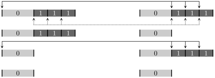
Figure 2. Illustration of the location of tiles within their level-$1$ supertiles for the proof of Proposition 3.2. The solid arrows on top of the lines indicate the pairing for intervals of types $0$ (left) and $1$ (right), the dashed arrows the pairings of two intervals of type $1$. The remaining two cases are analogous.

Proof.

Since our inflation rule is aperiodic, we have local recognisability [31]. This means that each tile in any (fixed) element of the hull lies inside a unique level-$1$ supertile that is identified by a local rule. Concretely, each patch of type $0111$ constitutes a supertile of type $0$, while each tile of type $0$ that is followed by another $0$ (to the right) stands for a supertile of type $1$. Below, we simply say supertile, as no level higher than $1$ will occur in this proof.

Due to the inflation structure, it is also clear that the relative frequency (meaning relative to $\varLambda$) of two supertiles of type $i$ and $j$ with distance $z$ (from $i$ to $j$) is given by $\frac{1}{\lambda}\hskip 0.5pt\nu_{ij}\bigl{(}\frac{z}{\lambda}\bigr{)}$. This follows from the simple observation that, for any $\varLambda\in\mathbb{Y}$, the point set of the left endpoints of the supertiles is a set of the form $\lambda\varLambda^{\prime}$ for some $\varLambda^{\prime}\in\mathbb{Y}$.

We can now relate the occurrences of pairs of tiles at distance $z$ to those of the supertiles they are in; see Figure 2 for an illustration. For instance, a distance $z$ between two tiles of type $0$ emerges once from any pair of supertiles (of either type) at the same distance. With the above formula for the relative frequency of the supertiles, this gives the first equation.

Likewise, the frequency $\nu_{01}(z)$ is composed of supertile frequencies of type $00$, at distances $(z-\lambda)$, $(z-\lambda-1)$ and $(z-\lambda-2)$, and supertile frequencies of type $10$, at the same set of distances; see Figure 2 for an explicit illustration. This gives the second equation. The remaining two identities are derived analogously.

The additional constraints are clear from Fact 3.1. ∎

3.2. Solution space

In view of our setting, it is clear that there is at least one solution of the (infinite) linear system of equations in Proposition 3.2, under the extra conditions stated there. Less obvious is the following, considerably stronger statement, where a larger support is admitted and no symmetry relation is prescribed.

Theorem 3.3.

Assume that $\nu_{ij}(z)=0$ for all $z\not\in\varDelta$ and all $i,j\in\{0,1\}$, and consider the subset of equations for $\nu_{ij}(z)$ that emerges from Proposition 3.2 by restricting to arguments $z\in\varDelta$ of modulus $|z|\leqslant 1+\lambda$. This is a finite and closed set of linear equations. The dimension of the solution space of all equations equals that of this finite subset.

In particular, the dimension of the solution space is $1$. Taking into account the requirement $\nu_{00}(0)+\nu_{11}(0)=1$ for the relative prototile frequencies, the solution is unique.

Proof.

Observe first that, when $\lvert z\rvert\leqslant\lambda+1$, no argument on the right-hand sides of the identities in Proposition 3.2 exceeds $\lambda+1$ in modulus. Since $\{z\in\varDelta:\lvert z\rvert\leqslant\lambda+1\}$ is a finite set and $\nu_{ij}(z)=0$ for any $z\not\in\varDelta$, the first claim is obvious. If, on the other hand, $\lvert z\rvert>\lambda+1$, all arguments on the right-hand sides are strictly smaller than $\lvert z\rvert$, wherefore all coefficients $\nu_{ij}(z)$ are determined by values at smaller arguments. Since $\varDelta$ is locally finite, the second claim follows from standard arguments.

Thus, only the equations for $\lvert z\rvert\in\{0,1,2,\lambda,3,1+\lambda\}$ need to be considered separately, as after that all frequencies are determined recursively. This gives $44$ linear equations that can be solved by standard methods, either by hand or by algebraic manipulation, the details of which we omit here. It turns out that $\nu_{00}(0)$ is not fixed by the relations, while all other function values can be written as a function of $\nu_{00}(0)$, with $\nu_{11}(0)=\frac{3}{\lambda}\hskip 0.5pt\nu_{00}(0)$ in particular. This means that the solution space is indeed one-dimensional. Imposing $\nu_{00}(0)+\nu_{11}(0)=1$ with $\nu_{00}(0)\geqslant 0$ results in $\nu_{00}(0)=1/\lambda$, so $\nu_{00}(0)=\nu_{0}$ and $\nu_{11}(0)=\nu_{1}$ with the frequencies from Eq. (2.3). All other values are then uniquely determined as listed in Table 1. We leave the details of this calculation to the reader. ∎

Table 1. Relative frequencies $\nu_{ij}(z)$ for all distances $z\in\varDelta$ with $|z|\leqslant 1+\lambda$.

$z$	$-1-\lambda$	$-3$	$-\lambda$	$-2$	$-1$	$0$	$1$	$2$	$\lambda$	$3$	$1+\lambda$
$\nu_{00}$	$0$	$0$	$3\lambda^{-3}$	$0$	$0$	$\lambda^{-1}$	$0$	$0$	$3\lambda^{-3}$	$0$	$0$
$\nu_{01}$	$\lambda^{-3}$	$\lambda^{-2}$	$0$	$\lambda^{-2}$	$\lambda^{-2}$	$0$	$0$	$0$	$\lambda^{-2}$	$0$	$\lambda^{-2}$
$\nu_{10}$	$\lambda^{-2}$	$0$	$\lambda^{-2}$	$0$	$0$	$0$	$\lambda^{-2}$	$\lambda^{-2}$	$0$	$\lambda^{-2}$	$\lambda^{-3}$
$\nu_{11}$	$3\lambda^{-4}$	$0$	$0$	$\lambda^{-2}$	$2\lambda^{-2}$	$3\lambda^{-2}$	$2\lambda^{-2}$	$\lambda^{-2}$	$0$	$0$	$3\lambda^{-4}$

Next, let us observe that each pair correlation function can uniquely be decomposed as $\nu_{ij}(z)=\nu^{+}_{ij}(z)+\nu^{-}_{ij}(z)$, with

$$\nu^{\pm}_{ij}(z)\,:=\,\frac{\raisebox{-2.0pt}{$1$}}{\raisebox{0.5pt}{$2$}}\,\bigl{(}\nu_{ij}(z)\pm\nu_{ji}(-z)\bigr{)},$$

into a symmetric and an anti-symmetric part. Since the right-hand sides of the renormalisation equations are linear and preserve the symmetry type, we may conclude as follows.

Corollary 3.4.

Under the assumptions of Theorem 3.3, all solutions of the renormalisation equations from Proposition 3.2 automatically satisfy the symmetry requirement of Proposition 3.2. In particular, the only anti-symmetric solution is the trivial one. ∎

Let us comment on these findings. While the renormalisation equations are a consequence of the structure of the hull $\mathbb{Y}$, it is by no means obvious that their solutions are essentially unique. This property was previously shown for the Fibonacci system in [2], but need not hold in general. In fact, uniqueness fails for the Thue–Morse system as soon as the support is enlarged, and this is then related to the existence of a spectrum of mixed type. To further analyse the (still more complex) situation in our non-PV point set, we need to reformulate the above findings in terms of measures and their Fourier transforms.

4. Pair correlation measures and their Fourier transforms

4.1. From functions to measures

Given the pair correlation functions $\nu_{ij}$, which have the locally finite point sets $S_{ij}$ as supports, we can turn them into positive pure point measures by defining

(4.1) $$\varUpsilon_{ij}\,:=\sum_{z\in S_{ij}}\nu_{ij}(z)\,\delta_{z}\hskip 0.5pt.$$

Together with Eq. (3.1), for any $0\leqslant i,j\leqslant 1$, this implies the relation

(4.2) $$\varUpsilon_{ij}\,=\,\frac{\widetilde{\delta_{\!\!\varLambda^{(i)}}}\!\circledast\delta_{\!\!\varLambda^{(j)}}}{\operatorname{\mathrm{dens}}(\varLambda)}\,=\,\frac{\delta_{-\varLambda^{(i)}}\!\circledast\delta_{\!\!\varLambda^{(j)}}}{\operatorname{\mathrm{dens}}(\varLambda)}\hskip 0.5pt,$$

as can be verified by an explicit calculation that is analogous to that for Eq. (2.8). Here, as before, $\varLambda\in\mathbb{Y}$ is arbitrary, but the result is independent of its choice due to Fact 3.1. Note that $\varUpsilon_{ij}\bigl{(}\{x\}\bigr{)}=\nu_{ij}(x)$ in this notation, and that Eq. (4.2) gives a first hint on an underlying tensor product structure. For this reason, as usual in multilinear algebra, we will sometimes view $\varUpsilon$ as a measure matrix, then written as $\bigl{(}\varUpsilon_{ij}\bigr{)}_{0\leqslant i,j\leqslant 1}$, or as a measure vector $(\varUpsilon_{00},\varUpsilon_{01},\varUpsilon_{10},\varUpsilon_{11})^{t}$ with lexicographic index ordering, whatever is better suited.

To expand on the last point, let us mention that the vector notation will have some advantage in the formulation of the measure-valued renormalisation relations to be derived shortly. On the other hand, let us observe that the matrix version is certainly useful for lifting Eq. (3.4) to the level of measures. If $(u_{0},u_{1})$ are the (complex) weights of the measure $\omega$ from Eq. (2.6), so $\omega=u_{0}\,\delta_{\!\!\varLambda_{\vphantom{a}}^{(0)}}+u_{1}\,\delta_{\!\!\varLambda_{\vphantom{a}}^{(1)}}$, the corresponding autocorrelation measure $\gamma_{u}$ can be written as

(4.3) $$\gamma_{u}(\mathcal{E})\,=\,\operatorname{\mathrm{dens}}(\varLambda)\!\!\sum_{i,j\in\{0,1\}}\!\!\overline{u_{i}}\;\varUpsilon_{ij}(\mathcal{E})\,u_{j}$$

where $\mathcal{E}\subset\mathbb{R}\hskip 0.5pt$ is any bounded Borel set. Note that $\omega$ is defined via a fixed $\varLambda\in\mathbb{Y}$, but that $\gamma_{u}$ does not depend on it by Proposition 2.2.

Each $\varUpsilon_{ij}$ is a positive pure point measure that is unbounded. It is translation bounded as a consequence of Eq. (4.2), because the Eberlein convolution of translation bounded measures is translation bounded again. Moreover, each $\varUpsilon_{ii}$ is positive definite, while the $\varUpsilon_{ij}$ for $i\neq j$ can be written as the (complex) linear combination of four positive definite measures by an application of the complex polarisation identity; compare [2, Lemma 1]. Consequently, each $\varUpsilon_{ij}$ is Fourier transformable as a measure [1], and we get the following result from the Bochner–Schwartz theorem; see [32, 13, 3] for background.

Fact 4.1.

Each pair correlation measure $\varUpsilon_{ij}$ from Eq. (4.2) is an unbounded, but translation bounded pure point measure with support $S_{ij}$. Moreover, it is Fourier transformable as a measure, and the transform $\widehat{\varUpsilon_{ij}}$ is a translation bounded and positive definite measure, which is also positive if $i=j$. ∎

At this point, we can Fourier transform Eq. (4.3) to obtain

(4.4) $$\widehat{\gamma_{u}}(\mathcal{E})\,=\,\operatorname{\mathrm{dens}}(\varLambda)\!\!\sum_{i,j\in\{0,1\}}\!\!\overline{u_{i}}\;\widehat{\varUpsilon}_{ij}(\mathcal{E})\,u_{j}$$

as a general formula of the diffraction measure of the weighted Dirac comb $\omega$ from Eq. (2.6) in terms of the Fourier transforms of the pair correlation measures, evaluated at a bounded Borel set $\mathcal{E}\subset\mathbb{R}\hskip 0.5pt$. This explains why further relations among the correlation measures will help to determine the spectral properties of the diffraction measure.

4.2. Renormalisation relations for measures

Now, we have to rewrite the renormalisation equations for the pair correlation functions from Proposition 3.2 in terms of the correlation measures $\varUpsilon_{ij}$. To do so, we employ the convolution with suitable finite measures. This is well-defined by standard results; see [13, Prop. 1.13]. To proceed, recall that we are working with prototiles (intervals) of natural lengths, namely $\lambda$ and $1$ for tiles of type $0$ and $1$, respectively. Define the set-valued location or displacement matrix $T=\bigl{(}T_{ij}\bigr{)}_{0\leqslant i,j\leqslant 1}$ by

$$T_{ij}\,:=\,\{\text{all relative positions of tiles of type $i$ in the supertile of type $j$}\}\hskip 0.5pt,$$

where the relative positions are again defined via the left endpoints of the tiles (intervals). Clearly, $\operatorname{\mathrm{card}}(T):=\bigl{(}\operatorname{\mathrm{card}}(T_{ij})\bigr{)}_{0\leqslant i,j\leqslant 1}=M$, and we have

$$T\,=\,\begin{pmatrix}\{0\}&\{0\}\\ \{\lambda,\lambda+1,\lambda+2\}&\varnothing\end{pmatrix}.$$

We now turn this into a matrix of finite measures (or Dirac combs) by setting

$$\delta_{\hskip 0.5ptT}\;:=\;\begin{pmatrix}\delta_{0}&\delta_{0}\\ \delta_{\lambda}+\delta_{\lambda+1}+\delta_{\lambda+2}&0\end{pmatrix}.$$

Next, define the scaling function (or dilation) $f$ on $\mathbb{R}\hskip 0.5pt$ by $f(z)=\lambda z$. Then, given $\mu$, the measure $f.\hskip 0.5pt\mu$ is defined by $\bigl{(}f.\hskip 0.5pt\mu\bigr{)}(g):=\mu(g\circ f)$ for $g\in C_{\mathsf{c}}(\mathbb{R}\hskip 0.5pt)$. In particular, this means $f.\hskip 0.5pt\hskip 0.5pt\delta_{z}=\delta_{f(z)}$. Using $\delta_{x}*\delta_{y}=\delta_{x+y}$ and the usual rules for a change of variable in weighted sums over Dirac measures, compare [2], one obtains the following result from a straight-forward calculation.

Lemma 4.2.

With $\varUpsilon_{ij}$ defined as in Eq. (4.2), the renormalisation equations from Proposition 3.2 are equivalent to the measure identity

$$\varUpsilon\,=\,\frac{\raisebox{-2.0pt}{$1$}}{\raisebox{0.5pt}{$\lambda$}}\,\Bigl{(}\hskip 0.5pt\widetilde{\delta_{T}}\stackrel{{\scriptstyle*}}{{\otimes}}\delta_{T}\Bigr{)}*(f.\hskip 0.5pt\hskip 0.5pt\varUpsilon)\hskip 0.5pt,$$

where $\varUpsilon$ is considered as a vector of pure point measures, $*$ denotes convolution of measures and $\stackrel{{\scriptstyle*}}{{\otimes}}$ the Kronecker convolution product. ∎

More generally, if $\mathcal{M}^{\infty}(\mathbb{R}\hskip 0.5pt)$ denotes the space of translation bounded measures on $\mathbb{R}\hskip 0.5pt$, one can define a linear mapping from $\mathcal{M}^{\infty}(\mathbb{R}\hskip 0.5pt)^{4}$ into itself by $Y\mapsto\Bigl{(}\hskip 0.5pt\widetilde{\delta_{T}}\stackrel{{\scriptstyle*}}{{\otimes}}\delta_{T}\Bigr{)}*(f.Y)$, which is continuous in the vague topology. Our measure vector $\varUpsilon\!$, as defined with the pair correlation functions $\nu_{ij}$ from Proposition 3.2 and Theorem 3.3, is then an eigenvector of this linear map, with eigenvalue $\lambda$. It might be an interesting question to analyse linear maps of this kind more systematically. Here, with $\mu_{\mathrm{L}}$ denoting Lebesgue measure on $\mathbb{R}\hskip 0.5pt$, we only mention that

(4.5) $$Y_{ij}\,:=\,\nu_{i}\,\nu_{j}\,\mu_{\mathrm{L}}$$

with the frequencies $\nu_{i}$ from Eq. (2.3) is another eigenvector. This can easily be checked from $\delta_{x}*\mu_{\mathrm{L}}=\mu_{\mathrm{L}}$ for any $x\in\mathbb{R}\hskip 0.5pt$ together with the observation that $v_{\mathrm{PF}}\otimes v_{\mathrm{PF}}$ is an eigenvector of $M\otimes M$, where $\otimes$ denotes the Kronecker product (see below for more). In fact, up to an overall constant, the $Y_{ij}$ from Eq. (4.5) form the only solution of the measure-valued renormalisation relation where each $Y_{ij}$ is a multiple of Lebesgue measure. We will return to this point later.

4.3. Renormalisation after Fourier transform

Now, we can turn the new relation from Lemma 4.2 into one on the Fourier side. For consistency with previous work [2], we define

$$B\,=\,\widehat{\widetilde{\delta_{T}}}\,=\,\widehat{\delta_{-T}}\,=\,\overline{\widehat{\delta_{T}}}\hskip 0.5pt,$$

where $B$ is a matrix of complex analytic functions because all elements of $\delta_{T}$ are finite measures with compact support; $B$ is called the Fourier matrix of the inflation rule. In line with common practice in this context, we use $k$ as the variable on the Fourier side, which is real-valued for our further analysis. Elementwise, we thus have

(4.6) $$B_{ij}(k)\,=\sum_{t\in T_{ij}}\,\mathrm{e}^{2\pi\hskip 0.5pt\mathrm{i}kt},$$

where $B(0)=M$. Now, with

(4.7) $$A(k)\,:=\,B(k)\otimes\overline{B(k)},$$

where the Kronecker product stands for the standard matrix representation of the tensor product with lexicographic ordering of the components, we can apply the convolution theorem to the identity in Lemma 4.2. Recalling further that $\widehat{f.\hskip 0.5pt\mu}=\frac{1}{\lambda}\,(f^{-1}.\hskip 0.5pt\widehat{\mu}\hskip 0.5pt)$ for our dilation $f$ and any transformable measure $\mu$, one obtains the following result.

Proposition 4.3.

Under Fourier transform, the identity of Lemma 4.2 turns into the relation

$$\widehat{\varUpsilon}\,=\,\frac{\raisebox{-2.0pt}{$1$}}{\raisebox{0.5pt}{$\lambda^{2}$}}\,A(.)\cdot\bigl{(}f^{-1}.\hskip 0.5pt\widehat{\varUpsilon}\hskip 0.5pt\hskip 0.5pt\bigr{)},$$

where $A(.)$ is the matrix function of Eq. (4.7), $f$ is the dilation defined by $f(x)=\lambda\hskip 0.5ptx$, and $\widehat{\varUpsilon}$ is the vector of Fourier transforms of the pair correlation measures. ∎

In analogy to above, one may view $\widehat{\varUpsilon}$ as an eigenvector of a linear mapping, this time with eigenvalue $\lambda^{2}$. Spelled out elementwise, with the double indices from the Kronecker product, the identity in Proposition 4.3 reads

$$\widehat{\varUpsilon}_{ij}\,=\sum_{m,n}A_{ij,mn}(.)\,\bigl{(}f^{-1}.\hskip 0.5pt\widehat{\varUpsilon}_{mn}\bigr{)}\hskip 0.5pt,$$

which also explains how the elements of the matrix $A$ appear as densities for the entries of the measure vector $\bigl{(}f^{-1}.\hskip 0.5pt\widehat{\varUpsilon}\hskip 0.5pt\hskip 0.5pt\bigr{)}$. Here, $A_{ij,mn}(k)=B_{im}(k)\,\overline{B_{jn}(k)}$ from the Kronecker product structure. This means that we can alternatively write the identity for $\widehat{\varUpsilon}$ in matrix form as

(4.8) $$\widehat{\varUpsilon}\,=\,\frac{\raisebox{-2.0pt}{$1$}}{\raisebox{0.5pt}{$\lambda^{2}$}}\,B(.)\bigl{(}f^{-1}.\hskip 0.5pt\widehat{\varUpsilon}\hskip 0.5pt\hskip 0.5pt\bigr{)}B^{{\dagger}}(.)\hskip 0.5pt,$$

where $B^{{\dagger}}$ denotes the Hermitian adjoint of $B$ and $\widehat{\varUpsilon}$ is considered as a $2\!\times\!2$-matrix. Both versions will be handy later on.

From this short derivation, is should be clear that the structure of the matrix functions $B(k)$ and $A(k)$ are important. We thus turn to a more detailed analysis of them, before we return to the renormalisation identities and their consequences for our spectral problem.

5. Inflation displacement algebra and Kronecker product extension

5.1. The inflation displacement algebra

Let us define the total set $S_{T}:=\bigcup_{i,j}T_{ij}$ of all relative locations of prototiles in level one supertiles, which means

$$S_{T}\,=\,\{0,\lambda,\lambda+1,\lambda+2\}\hskip 0.5pt.$$

Then, we can decompose the Fourier matrices $B(k)$ from Eq. (4.6) as

(5.1) $$B(k)\,=\sum_{x\in S_{T}}\,\mathrm{e}^{2\pi\hskip 0.5pt\mathrm{i}kx}D_{x}$$

with integer $0\hskip 0.5pt\hskip 0.5pt$-$1$-matrices $D_{x}$ that satisfy $\sum_{x\in S_{T}}D_{x}=M$. Explicitly, we have

(5.2) $$D_{0}\,=\,\begin{pmatrix}1&1\\ 0&0\end{pmatrix}\quad\text{and}\quad D_{\lambda}\,=\,D_{\lambda+1}\,=\,D_{\lambda+2}\,=\,\begin{pmatrix}0&0\\ 1&0\end{pmatrix},$$

where the matrix elements are given by

$$D_{x,ij}\,=\,\begin{cases}1,&\text{if the supertile of type $j$ contains a tile of type $i$ at $x$},\\ 0,&\text{otherwise}\hskip 0.5pt.\end{cases}$$

These geometric incidence matrices are a generalisation of what is known as digit matrices in constant length substitutions [37, 21], wherefore we adopt this terminology here as well; compare also [31, Sec. 8.1]. Recently, also the term instruction matrices has been used [11].

Next, consider the $\mathbb{C}\hskip 0.5pt$-algebra $\mathcal{B}$ that is generated by the one-parameter matrix family $\{B(k):k\in\mathbb{R}\hskip 0.5pt\}$. We call this finite-dimensional algebra, which is automatically closed, the inflation displacement algebra (IDA) of $\varrho$. Consider also the $\mathbb{C}\hskip 0.5pt$-algebra $\mathcal{B}_{D}$ that is generated by the digit matrices $\{D_{x}:x\in S_{T}\}$, hence by $D_{0}$ and $D_{\lambda}$ in our case. Recall that a family of $2\!\times\!2$-matrices is called irreducible (over the field $\mathbb{C}\hskip 0.5pt$) if the only subspaces of $\mathbb{C}\hskip 0.5pt^{2}$ that are invariant under all elements of the matrix family are the trivial subspaces, $\{0\}$ and $\mathbb{C}\hskip 0.5pt^{2}$.

Lemma 5.1.

The IDA of $\varrho$ satisfies $\mathcal{B}=\mathcal{B}_{D}=\mathrm{Mat}(2,\mathbb{C}\hskip 0.5pt)$, which is also the IDA of $\varrho^{n}$ for any $n\in\mathbb{N}$. In particular, $\mathcal{B}_{D}$ is irreducible. For any $\varepsilon>0$, the complex algebra generated by the matrix family $\{B(k):0\leqslant k<\varepsilon\}$ is again $\mathcal{B}$. In fact, any finite set of matrices $\{B(k):k\in J\}$ generates $\mathcal{B}$, if $J$ contains at least two elements at which the trigonometric polynomial $p(k)=\,\mathrm{e}^{2\pi\hskip 0.5pt\mathrm{i}k\lambda}+\,\mathrm{e}^{2\pi\hskip 0.5pt\mathrm{i}k(\lambda+1)}+\,\mathrm{e}^{2\pi\hskip 0.5pt\mathrm{i}k(\lambda+2)}=\,\mathrm{e}^{2\pi\hskip 0.5pt\mathrm{i}k(\lambda+1)}\bigl{(}1+2\hskip 0.5pt\cos(2\pi k)\bigr{)}$ differs.

Proof.

From Eq. (5.2), we already know that the digit matrices for $\varrho$ are $D_{0}=E_{00}+E_{01}$ and $D_{\lambda}=E_{10}$ with $E_{ij}$ denoting the standard elementary matrices, indexed with $i,j\in\{0,1\}$ to match the labelling of the tile types. Observing that $D_{0}\hskip 0.5ptD_{\lambda}=E_{00}$ and $D_{\lambda}D_{0}=E_{10}+E_{11}$, we get $E_{01}$ and $E_{11}$ via differences. We thus have all four elementary matrices $E_{ij}$ within $\mathcal{B}_{D}$. This implies $\mathcal{B}_{D}=\mathrm{Mat}(2,\mathbb{C}\hskip 0.5pt)$, which is irreducible.

Next, one checks that $D_{0}$ and $D_{\lambda}$ are always among the digit matrices for $\varrho^{n}$ with $n\in\mathbb{N}$, hence we always get the full matrix algebra, $\mathrm{Mat}(2,\mathbb{C}\hskip 0.5pt)$.

The last claim, and then also the previous one, follows from the observation that Eq. (5.1), in view of the second identity in Eq. (5.2), can be rewritten as $B(k)=D_{0}+p(k)\hskip 0.5ptD_{\lambda}$. Thus, knowing $B(k)$ for $k_{1}$ and $k_{2}$ with $p(k_{1})\neq p(k_{2})$, we have a system of two equations that can be solved for $D_{0}$ and $D_{\lambda}$. This also implies $\mathcal{B}_{D}\subseteq\mathcal{B}$, while $\mathcal{B}\subseteq\mathcal{B}_{D}$ is clear from Eq. (5.1), so $\mathcal{B}=\mathcal{B}_{D}$ as stated. ∎

For later reference, we note that the matrix $B(k)$ can now be written as

(5.3) $$B(k)\,=\,\begin{pmatrix}1&1\\ p(k)&0\end{pmatrix},$$

where $p$ is the trigonometric polynomial from Lemma 5.1. Let us state an elementary observation that will later give us access to a compactness argument; see [3, Ex. 8.1] and references given there for background on quasiperiodic functions.

Fact 5.2.

The polynomial $p$ from Lemma  5.1 is quasiperiodic, with fundamental frequencies $1$ and $\lambda$. As such, it can be represented as

$$p(k)\,=\,\tilde{p}(x,y)\big{|}_{x=\lambda k,\,y=k}$$

with $\tilde{p}(x,y):=\,\mathrm{e}^{2\pi\hskip 0.5pt\mathrm{i}(x+y)}\hskip 0.5pt\bigl{(}1+2\cos(2\pi y)\bigr{)}$, which is $1$-periodic in both arguments. In this representation, one has

$$p(\lambda k)\,=\,\tilde{p}\bigl{(}(x,y)M\bigr{)}\big{|}_{x=\lambda k,\,y=k}\hskip 0.5pt=\,\tilde{p}(x+3y,x)\big{|}_{x=\lambda k,\,y=k}$$

with the substitution matrix $M$ from Eq. (2.2). Likewise, $B(k)$ defines a quasiperiodic matrix function, with $B(k)=\tilde{B}(x,y)\big{|}_{x=\lambda k,\,y=k}$ and $\tilde{B}(x,y)=\left(\begin{smallmatrix}1&1\\ \tilde{p}(x,y)&0\end{smallmatrix}\right)$.

Proof.

The first claim is clear, while the second follows from the fact that $(\lambda,1)$ is the left PF eigenvector of $M$; this relation motivated the particular representation we chose.

The consequence for $B$ is now obvious. ∎

5.2. Kronecker products

Let us consider the matrix function $A(k)=B(k)\otimes\overline{B(k)}$ introduced above in Eq. (4.7), with $B(k)$ as in Eq. (5.3). This somewhat unusual product with complex conjugation reflects, on the Fourier side, the symmetry relation $\nu_{ji}(z)=\nu_{ij}(-z)$ from Proposition 3.2. So, consider the matrix family $\{{A}(k):k\in\mathbb{R}\hskip 0.5pt\}$ or any (possibly finite, but sufficiently large) subset of it. Even though the IDA $\mathcal{B}$ is irreducible, this does not transfer to the ${A}$-matrices, as is well-known from representation theory. Indeed, let $V=\mathbb{C}\hskip 0.5pt^{2}$ and consider $W:=V\otimes_{\mathbb{C}\hskip 0.5pt}V$, the (complex) tensor product. $W$ is a vector space over $\mathbb{C}\hskip 0.5pt$ of dimension $4$, but also one over $\mathbb{R}\hskip 0.5pt$, then of dimension $8$.

Now, view $W$ as an $\mathbb{R}\hskip 0.5pt$-vector space and consider the involution $C\!:\,W\longrightarrow W$ defined by

$$x\otimes y\;\longmapsto\;C(x\otimes y):=\overline{y\otimes x}=\bar{y}\otimes\bar{x}$$

together with its unique extension to an $\mathbb{R}\hskip 0.5pt$-linear mapping on $W$. Note that there is no $\mathbb{C}\hskip 0.5pt$-linear extension, because $C\bigl{(}a(x\otimes y)\bigr{)}=\bar{a}\,C(x\otimes y)$ for $a\in\mathbb{C}\hskip 0.5pt$. From the definition, one finds

$$\begin{split}{A}(k)\,C(x\otimes y)\,&=\,\bigl{(}B(k)\otimes\,\overline{\!B(k)\!}\,\bigr{)}(\bar{y}\otimes\bar{x})\,=\,\bigl{(}B(k)\hskip 0.5pt\bar{y}\bigr{)}\otimes\bigl{(}\,\overline{\!B(k)\hskip 0.5ptx}\,\bigr{)}\\ &=\,C\left(\bigl{(}B(k)\otimes\,\overline{\!B(k)\!}\,\bigr{)}(x\otimes y)\right)\,=\,C\bigl{(}{A}(k)\,(x\otimes y)\bigr{)},\end{split}$$

so $C$ commutes with the linear map defined by ${A}(k)$, for any $k\in\mathbb{R}\hskip 0.5pt$. The eigenvalues of $C$ are $\pm 1$, and our vector space splits as $W\!=W_{\!+}\oplus W_{\!-}$ into real vector spaces that are the eigenspaces of $C$, so $W_{\!\pm}=\{x\in W:C(x)=\pm\hskip 0.5ptx\}$. Their dimensions are

$$\dim_{\mathbb{R}\hskip 0.5pt}(W_{\!+})\,=\,\dim_{\mathbb{R}\hskip 0.5pt}(W_{\!-})\,=\,4$$

since $W_{\!-}=\hskip 0.5pt\mathrm{i}\hskip 0.5ptW_{\!+}$ with $W_{\!+}\cap W_{\!-}=\{0\}$. The corresponding splitting of an arbitrary $w\in W$ is unique and given by $w=\frac{1}{2}\bigl{(}w+C(w)\bigr{)}+\frac{1}{2}\bigl{(}w-C(w)\bigr{)}$ as usual.

It is now clear that $W_{\!+}$ and $W_{\!-}$ are invariant (real) subspaces of our matrix family, and of the $\mathbb{R}\hskip 0.5pt$-algebra ${\mathcal{A}}$ generated by it. Fortunately, due to the symmetry relation for the correlation coefficients, the irreducibility of $\mathcal{A}$ on the subspace $W_{\!+}$ is what matters later on.

Let us pause to observe a connection with the digit matrices. We have

$${A}(k)\,=\,B(k)\otimes\overline{B(k)}\;=\!\sum_{x,y\in S_{T}}\!\,\mathrm{e}^{2\pi\hskip 0.5pt\mathrm{i}k(x-y)}\,D_{x}\otimes D_{y}\;=\sum_{z\in S_{T}-S_{T}}\,\mathrm{e}^{2\pi\hskip 0.5pt\mathrm{i}kz}\,F_{z}$$

where

$$F_{z}\;=\sum_{\begin{subarray}{c}x,y\in S_{T}\\ x-y=z\end{subarray}}D_{x}\otimes D_{y}\hskip 0.5pt.$$

In particular, one has

$$F_{0}\,=\,\begin{pmatrix}1&1&1&1\\ 0&0&0&0\\ 0&0&0&0\\ 3&0&0&0\end{pmatrix}$$

with spectrum $\{\lambda,\lambda^{\prime},0,0\}$, while all $F_{z}$ with $0\neq z\in S_{T}-S_{T}$ are nilpotent, with $F_{z}^{2}=0$. Now, one easily checks that $\bigl{(}C(a\hskip 0.5ptF_{z})\hskip 0.5ptC\bigr{)}(u\otimes v)=\bar{a}\,F_{-z}(u\otimes v)$, which implies $\bigl{[}C,{A}(k)\bigr{]}=0$ for all $k\in\mathbb{R}\hskip 0.5pt$, in line with our previous derivation.

Lemma 5.3.

The $\mathbb{R}\hskip 0.5pt$-algebra ${\mathcal{A}}$ satisfies $\dim_{\mathbb{R}\hskip 0.5pt}({\mathcal{A}})=16$ and acts irreducibly on each of the invariant four-dimensional subspaces $W_{\!+}$ and $W_{\!-}$ introduced above.

Proof.

We will show that ${\mathcal{A}}\simeq\mathrm{Mat}(4,\mathbb{R}\hskip 0.5pt)$. If one considers $\mathrm{Mat}(4,\mathbb{C}\hskip 0.5pt)$ as an $\mathbb{R}\hskip 0.5pt$-algebra of dimension $32$, the subalgebra ${\mathcal{A}}$ consists of all elements that are fixed under the $\mathbb{R}\hskip 0.5pt$-linear mapping defined by $M_{1}\otimes M_{2}\mapsto\overline{M_{2}}\otimes\overline{M_{1}}$. Consequently, with $E_{ij,k\ell}:=E_{ik}\otimes E_{j\ell}$, a basis of the $\mathbb{R}\hskip 0.5pt$-algebra ${\mathcal{A}}$ as a $16$-dimensional real vector space can be constructed from the spanning set

$$\bigl{\{}\tfrac{1}{2}(E_{ij,k\ell}+E_{ji,\ell k}):i,j,k,\ell\in\{0,1\}\bigr{\}}\cup\bigl{\{}\tfrac{\hskip 0.5pt\mathrm{i}}{2}(E_{ij,k\ell}-E_{ji,\ell k}):i,j,k,\ell\in\{0,1\}\bigr{\}},$$

where the first resp. second subset contains $10$ resp. $6$ linearly independent elements.

Next, consider the unitary matrix

(5.4) $$U\,=\,\frac{1}{\sqrt{2}}\begin{pmatrix}1\!-\!\hskip 0.5pt\mathrm{i}&0&0&0\\ 0&1&-\hskip 0.5pt\mathrm{i}&0\\ 0&-\hskip 0.5pt\mathrm{i}&1&0\\ 0&0&0&1\!-\!\hskip 0.5pt\mathrm{i}\end{pmatrix},$$

which acts on $\mathrm{Mat}(4,\mathbb{C}\hskip 0.5pt)$ via conjugation $(.)\mapsto U(.)\hskip 0.5pt\hskip 0.5ptU^{-1}$. When applied to the basis matrices of ${\mathcal{A}}$, one obtains $16$ real matrices which, by suitable integer linear combinations, yield all $16$ elementary matrices $E_{ij,k\ell}$. Therefore, within $\mathrm{Mat}(4,\mathbb{C}\hskip 0.5pt)$, ${\mathcal{A}}$ is conjugate to $\mathrm{Mat}(4,\mathbb{R}\hskip 0.5pt)$. This implies that the action of ${\mathcal{A}}$ on the invariant subspaces $W_{\!+}$ and $W_{\!-}$ is irreducible. ∎

5.3. Consequences

Observe next that $[U,{A}(0)]=0$ and that $U(W_{\!\mp})=\frac{1{\scriptscriptstyle\pm}\hskip 0.5pt\mathrm{i}}{\sqrt{2}}\,\mathbb{R}\hskip 0.5pt^{4}$. Moreover,

$${A}_{U}(k)\,:=\,U{A}(k)\,U^{-1}\,=\,\begin{pmatrix}1&1&1&1\\ c(k)+s(k)&s(k)&c(k)&0\\ c(k)-s(k)&c(k)&-s(k)&0\\ c(k)^{2}+s(k)^{2}&0&0&0\end{pmatrix}$$

with

$$\begin{split}c(k)&\,=\,\cos(2\pi\lambda k)+\cos(2\pi(\lambda\!+\!1)k)+\cos(2\pi(\lambda\!+\!2)k)\hskip 0.5pt,\\ s(k)&\,=\,\sin(2\pi\lambda k)\hskip 0.5pt+\hskip 0.5pt\sin(2\pi(\lambda\!+\!1)k)\hskip 0.5pt+\hskip 0.5pt\sin(2\pi(\lambda\!+\!2)k)\hskip 0.5pt,\end{split}$$

so that $c(k)^{2}+s(k)^{2}=\bigl{|}p(k)\bigr{|}^{2}=\bigl{(}1+2\cos(2\pi k)\bigr{)}^{2}$ and ${A}_{U}(0)={A}(0)=M\otimes M$ with the substitution matrix $M$ from Eq. (2.2). Since ${A}_{U}(0)^{2}$ is a strictly positive integer matrix, and since ${A}_{U}(\frac{k}{\lambda})\hskip 0.5pt{A}_{U}(k)$ is continuous in $k$, the latter product is strictly positive as well for sufficiently small $k$. As one can easily calculate numerically, the smallest $k>0$ for which one element of ${A}_{U}(\frac{k}{\lambda})\hskip 0.5pt{A}_{U}(k)$ vanishes (and strict positivity is thus violated) is $k\approx 0.03832\hskip 0.5pt(1)$, so the product is certainly a strictly positive matrix for all $k\in[0,\varepsilon]$ with $\varepsilon=0.03$ say. Moreover, ${A}_{U}(k)$ cannot have zero eigenvalues for any $k$ with $\lvert k\rvert<\frac{1}{3}$, as follows from a simple determinant argument (see the proof of Lemma 6.4 below for details).

Proposition 5.4.

Let $k\in[0,\varepsilon]$ with this choice of $\varepsilon$, and consider the iteration

$$w_{n}\,:=\,\Bigl{(}{A}_{U}\bigl{(}\tfrac{k}{\lambda^{2n-1}}\bigr{)}\hskip 0.5pt{A}_{U}\bigl{(}\tfrac{k}{\lambda^{2n-2}}\bigr{)}\Bigr{)}\cdot\ldots\cdot\Bigl{(}{A}_{U}\bigl{(}\tfrac{k}{\lambda}\bigr{)}\hskip 0.5pt{A}_{U}\bigl{(}k\bigr{)}\Bigr{)}\hskip 0.5ptw_{0}$$

for $n\geqslant 1$ and any non-negative starting vector $w_{0}\neq 0$. Then, the vector $w_{n}$ will be strictly positive for all $n\in\mathbb{N}$ and, as $n\to\infty$, it will diverge with asymptotic growth $c\hskip 0.5pt\lambda^{4n}\hskip 0.5ptw_{\mathrm{PF}}$. Here, $c$ is a constant that depends on $w_{0}$ and $k$, while $w_{\mathrm{PF}}=v_{\mathrm{PF}}\otimes v_{\mathrm{PF}}$ is the statistically normalised PF eigenvector of $M\otimes M$ derived from Eq. (2.3).

Proof.

For $k=0$, this is standard Perron–Frobenius theory for the non-negative and primitive matrix ${A}(0)=M\otimes M$, which has PF eigenvalue $\lambda^{2}$ with eigenvector $w_{\mathrm{PF}}$. In particular, $A(0)^{2}$ is strictly positive. Since $w_{0}$ must have a component in the direction of $w_{\mathrm{PF}}$, this component leads to the asymptotic behaviour claimed.

For $0<k\leqslant\varepsilon$, one iterates with strictly positive matrices due to the choice of $\varepsilon$, so $w_{0}\neq 0$ means that $w_{1}$ is already strictly positive. Clearly, ${A}_{U}(\frac{k}{\lambda^{2n-1}})\hskip 0.5pt{A}_{U}(\frac{k}{\lambda^{2n-2}})$ is analytic in $k$ and converges to ${A}(0)^{2}$ as $n\to\infty$. No cancellation can occur in the iteration and, asymptotically, each iteration step multiplies the component in the direction of $w_{\mathrm{PF}}$ by $\lambda^{4}$. Due to the existence of a spectral gap for ${A}(0)^{2}$, this component dominates, and the claim follows. ∎

Let us formulate a simple consequence that will be useful in our later analysis.

Corollary 5.5.

Under the assumptions and in the setting of Proposition 5.4, consider the iteration

$$w^{\hskip 0.5pt\prime}_{m}\,=\,\frac{\raisebox{-2.0pt}{$1$}}{\raisebox{0.5pt}{$\lambda$}}\hskip 0.5pt{A}_{U}\bigl{(}\tfrac{k_{0}}{\lambda^{m}}\bigr{)}\,w^{\hskip 0.5pt\prime}_{m-1}$$

for $m\in\mathbb{N}$, with $k_{0}\in[0,\varepsilon]$ and $w^{\hskip 0.5pt\prime}_{0}=w_{0}$. Then, $w^{\hskip 0.5pt\prime}_{m}\sim c\hskip 0.5pt\lambda^{m}\,w_{\mathrm{PF}}$ as $m\to\infty$, where the constant $c$ depends on $w_{0}$ and $k_{0}$ as before. In other words, when viewing $w^{\hskip 0.5pt\prime}_{m}$ as a function $w^{\hskip 0.5pt\prime}$ evaluated at $k=k_{0}/\lambda^{m}$, one has

$$w^{\hskip 0.5pt\prime}(k)\,\sim\,\frac{\raisebox{-2.0pt}{$c$}}{\raisebox{0.5pt}{$k$}}\,w_{\mathrm{PF}}\quad\text{as $k\to 0$}$$

along the sequence $\bigl{(}k_{0}/\lambda^{m}\bigr{)}_{m\in\mathbb{N}_{0}}$. ∎

We now have the necessary tools to return to the analysis of the pair correlation measures and their Fourier transforms.

6. Renormalisation analysis of pair correlation measures

6.1. Lebesgue decomposition and consequences

The measure vector $\widehat{\varUpsilon}$ satisfies the renormalisation equation from Proposition 4.3. Each measure $\widehat{\varUpsilon}_{ij}$ has a unique Lebesgue decomposition

$$\widehat{\varUpsilon}_{ij}\,=\,\bigl{(}\widehat{\varUpsilon}_{ij}\bigr{)}_{\mathsf{pp}}+\bigl{(}\widehat{\varUpsilon}_{ij}\bigr{)}_{\mathsf{cont}}\,=\,\bigl{(}\widehat{\varUpsilon}_{ij}\bigr{)}_{\mathsf{pp}}+\bigl{(}\widehat{\varUpsilon}_{ij}\bigr{)}_{\mathsf{sc}}+\bigl{(}\widehat{\varUpsilon}_{ij}\bigr{)}_{\mathsf{ac}}$$

into a pure point and a continuous part, where the latter can further be decomposed into a singular continuous and an absolutely continuous part relative to Lebesgue measure. By standard arguments, this can be extended to the vector measure $\widehat{\varUpsilon}$ in such a way that the supporting sets of the three parts coincide for all $\widehat{\varUpsilon}_{ij}$.

Lemma 6.1.

Each spectral component of $\widehat{\varUpsilon}$ satisfies the renormalisation relation of Proposition 4.3 separately, which means that

$$\bigl{(}\widehat{\varUpsilon}\hskip 0.5pt\hskip 0.5pt\bigr{)}_{\mathsf{t}}\;=\;\frac{\raisebox{-2.0pt}{$1$}}{\raisebox{0.5pt}{$\lambda^{2}$}}\,{A}(.)\cdot\bigl{(}f^{-1}.\,(\widehat{\varUpsilon}\hskip 0.5pt)_{\mathsf{t}}\bigr{)}$$

holds for each spectral type $\mathsf{t}\in\{\mathsf{pp},\mathsf{sc},\mathsf{ac}\}$.

Proof.

Observe that the dilated measure $f^{-1}.\hskip 0.5pt\mu$ has the same spectral type as $\mu$, and that the matrix function ${A}(k)$ is analytic, so cannot mix different spectral types, which are mutually orthogonal in the measure-theoretic sense; compare [3, Prop. 8.4]. Consequently, for any $\mathsf{t}\in\{\mathsf{pp},\mathsf{sc},\mathsf{ac}\}$, one has

$$\Bigl{(}\frac{\raisebox{-2.0pt}{$1$}}{\raisebox{0.5pt}{$\lambda^{2}$}}\,{A}(.)\cdot\bigl{(}f^{-1}.\hskip 0.5pt\widehat{\varUpsilon}\hskip 0.5pt\hskip 0.5pt\bigr{)}\!\Bigr{)}_{\!\mathsf{t}}\,=\,\frac{\raisebox{-2.0pt}{$1$}}{\raisebox{0.5pt}{$\lambda^{2}$}}\,{A}(.)\cdot\left(f^{-1}.\,(\widehat{\varUpsilon}\hskip 0.5pt)_{\mathsf{t}}\right).$$

The claim now follows from the linearity of the renormalisation relation for $\widehat{\varUpsilon}$. ∎

Let us next observe that we have $\widehat{\varUpsilon}_{ij}=\widehat{\varUpsilon_{ij}}$ by definition, and that $\bigl{(}\widehat{\varUpsilon}_{ij}\bigr{)}$ is Hermitian as a matrix, because

$$\overline{\widehat{\varUpsilon_{ij}}}\,=\,\widehat{\widetilde{\varUpsilon_{ij}}}\,=\,\widehat{\varUpsilon_{ji}}\hskip 0.5pt.$$

If we combine this with Eq. (4.4) for $\widehat{\gamma_{u}}$, which is a positive measure for any complex weight vector $u$, we get the following property.

Fact 6.2.

For any bounded Borel set $\mathcal{E}\subset\mathbb{R}\hskip 0.5pt$, the complex matrix $\bigl{(}\widehat{\varUpsilon}_{ij}(\mathcal{E})\bigr{)}_{0\leqslant i,j\leqslant 1}$ is Hermitian and positive semi-definite. Since $\widehat{\varUpsilon}_{\!00}$ and $\widehat{\varUpsilon}_{\!11}$ are positive measures, positive semi-definiteness is equivalent to the determinant condition $\det\bigl{(}\widehat{\varUpsilon}_{ij}(\mathcal{E})\bigr{)}^{\vphantom{I}}\geqslant 0$. ∎

6.2. Renormalisation for pure point part

Let us further explore the meaning of the relation from Lemma 6.1. Clearly, the pure point part of $\widehat{\varUpsilon}$ is of the form

$$\bigl{(}\widehat{\varUpsilon}\hskip 0.5pt\hskip 0.5pt\bigr{)}_{\mathsf{pp}}\,=\,\sum_{k\in K}\mathcal{I}(k)\hskip 0.5pt\delta_{k}\hskip 0.5pt,$$

with $\mathcal{I}(k)=\widehat{\varUpsilon}\bigl{(}\{k\}\bigr{)}$. Here, $\bigl{(}\mathcal{I}_{ij}(k)\bigr{)}_{0\leqslant i,j\leqslant 1}$ is Hermitian and positive semi-definite as a consequence of Fact 6.2, and $K$ is at most a countable subset of $\mathbb{R}\hskip 0.5pt$, where $\lambda K\subset K$ may be assumed. Inserting $\bigl{(}\widehat{\varUpsilon}\hskip 0.5pt\hskip 0.5pt\bigr{)}_{\mathsf{pp}}$ into the relation from Lemma 6.1 leads, after some calculations, to the relation

(6.1) $$\mathcal{I}(k)\,=\,\frac{\raisebox{-2.0pt}{$1$}}{\raisebox{0.5pt}{$\lambda^{2}$}}\hskip 0.5pt{A}(k)\,\mathcal{I}(\lambda k)\hskip 0.5pt,$$

which has to hold for all $k\in K$. In particular, for $k=0$, one has

$${A}(0)\,\mathcal{I}(0)\,=\,\lambda^{2}\,\mathcal{I}(0)\hskip 0.5pt,$$

where $\lambda^{2}$ is the PF eigenvalue of ${A}(0)=M\otimes M$. This, with Eq. (2.7), implies

(6.2) $$\widehat{\varUpsilon}_{ij}\bigl{(}\{0\}\bigr{)}\,=\,\mathcal{I}_{ij}(0)\,=\,\nu_{i}\,\nu_{j}\,=\,\frac{\operatorname{\mathrm{dens}}(\varLambda^{(i)})\hskip 0.5pt\operatorname{\mathrm{dens}}(\varLambda^{(j)})}{\bigl{(}\operatorname{\mathrm{dens}}(\varLambda)\bigr{)}^{2}}\hskip 0.5pt,$$

where we employed the PF eigenvector of $A(0)$ together with the normalisation condition $\sum_{i,j}\mathcal{I}_{ij}(0)=1$, the latter being a consequence of our setting with relative frequencies; compare [3, Cor. 9.1] for the underlying calculation. Note that Eq. (6.2) also means that the Hermitian $2\!\times\!2$-matrix $\bigl{(}\mathcal{I}_{ij}(0)\bigr{)}$ has rank $1$. Moreover, Theorem 2.3 implies that $\mathcal{I}(k)=0$ for all $k\neq 0$, because otherwise Eq. (4.4) would give $\widehat{\gamma_{u}}\bigl{(}\{k\}\bigr{)}=\operatorname{\mathrm{dens}}(\varLambda^{w})\sum_{i,j}\overline{u_{i}}\;\mathcal{I}_{ij}(k)\,u_{j}>0$ for a suitable choice of the weights, in contradiction to Theorem 2.3. Consequently, we have

(6.3) $$\bigl{(}\widehat{\varUpsilon}\hskip 0.5pt\bigr{)}_{\mathsf{pp}}\,=\,\mathcal{I}(0)\,\delta_{0}$$

and the pure point part of $\widehat{\varUpsilon}$ is completely determined this way.

Remark 6.3.

Let us relate Eq. (6.3) back to the measure vector $Y$ from Eq. (4.5). With hindsight, $Y$ is the strongly almost periodic part of the Eberlein decomposition [22, 30] of $\varUpsilon$, so that $\widehat{Y}=\bigl{(}\widehat{\varUpsilon}\hskip 0.5pt\bigr{)}_{\mathsf{pp}}$. Note that any $Y_{ij}$ is an absolutely continuous measure with support $\mathbb{R}\hskip 0.5pt$, and thus not a pure point measure as in the case of the Fibonacci chain in [2]. This is related to the set $\varDelta$ from Proposition 2.1 not being uniformly discrete, and is the deeper reason why our discrete equations in Proposition 3.2 cannot produce a spectral purity result. $\Diamond$

6.3. Analysis of absolutely continuous part

Next, let $h_{ij}$ be the Radon–Nikodym density for $\bigl{(}\widehat{\varUpsilon}_{ij}\bigr{)}_{\mathsf{ac}}$, and $h$ the corresponding vector of densities. Each component is a locally integrable function on the real line. Another application of Lemma 6.1, together with an elementary transformation of variable calculation, which changes the scalar prefactor, then reveals the identity

(6.4) $${h}\bigl{(}\tfrac{k}{\lambda}\bigr{)}\,=\,\frac{\raisebox{-2.0pt}{$1$}}{\raisebox{0.5pt}{$\lambda$}}\hskip 0.5pt{A}\bigl{(}\tfrac{k}{\lambda}\bigr{)}\,{h}(k)\hskip 0.5pt,$$

which must hold for Lebesgue-almost every (a.e.) $k\in\mathbb{R}\hskip 0.5pt$. An iteration gives

(6.5) $${h}\bigl{(}\tfrac{k}{\lambda^{n}}\bigr{)}\,=\,\frac{\raisebox{-2.0pt}{$1$}}{\raisebox{0.5pt}{$\lambda^{n}$}}{A}\bigl{(}\tfrac{k}{\lambda^{n}}\bigr{)}\cdot\ldots\cdot{A}\bigl{(}\tfrac{k}{\lambda}\bigr{)}\,{h}(k)$$

for any $n\in\mathbb{N}$ and still almost every $k\in\mathbb{R}\hskip 0.5pt$. We thus obtain a matrix Riesz product type consistency equation for ${h}$, which can also be viewed as a (complex) linear cocycle for the mapping defined by $k\mapsto k/\lambda$ on $\mathbb{R}\hskip 0.5pt_{+}$.

Let us pause to explain the idea behind our ensuing analysis. Iterating a vector $h(k)$ inwards via Eq. (6.5) means that, asymptotically, we multiply with a matrix from the left that more and more looks like $A(0)=M\otimes M$. Since the leading eigenvalue is then (almost) $\lambda^{2}$, and we divide only by a single factor of $\lambda$, a component in the direction of $w_{\mathrm{PF}}$ (provided it exists) gets approximately multiplied by $\lambda$ in each iteration step. Consequently, we get a ‘blow-up’ of $h(k)$ along the (inward) iteration sequence, which means an asymptotic growth as $k^{-1}$ for $k\searrow 0$. Clearly, such a behaviour is impossible for a locally integrable function; see also Appendix B for an illustration in a one-dimensional analogue.

There are two mechanisms to avoid the blow-up: Either $h$ vanishes for a.e. $k\in\mathbb{R}\hskip 0.5pt$, or $h(k)$ is of a form that asymptotically avoids the direction of $w_{\mathrm{PF}}$. The first option is what we are after, while the second is connected with the Lyapunov spectrum of our iteration. As we shall see, the second possibility still occurs, and must be ruled out by the analysis of the asymptotic behaviour in an inverted (outward) iteration, so that we finally get $h=0$ in the Lebesgue sense, which means $\bigl{(}\widehat{\varUpsilon}\hskip 0.5pt\hskip 0.5pt\bigr{)}_{\mathsf{ac}}=0$. The actual line of arguments to make this strategy work is a bit delicate and technical, and will require a number of steps.

The rough outline of our arguments is as follows. The goal is to show that $h$ vanishes, and we only need to do so on a small interval (Lemma 6.4). With the extra hermiticity and rank structure of the matrix $(h_{ij})$ from Lemma 6.5, we gain a dimensional reduction, via Fact 6.6. This allows us to work with the Fourier matrices rather than their Kronecker products, where we profit from the algebraic structure derived earlier. In Proposition 6.7, we derive an asymptotic result on the determinants for the iterated application of our recursion that will later lead to an important relation between the Lyapunov exponents of our iteration.

The next step consists in the analysis of the inward iteration, which gives interesting insight (Proposition 6.8), but does not suffice to derive $h=0$. The main step then consists in deriving the (pointwise) Lyapunov exponents for the outward iteration (Proposition 6.17) and to show that they are both strictly positive (Corollary 6.19), which is incompatible with the translation boundedness of the diffraction measure. This will then lead to the desired conclusion that $h=0$ in the Lebesgue sense in Theorem 6.20, and to the determination of $\widehat{\varUpsilon}_{ij}$ in Corollary 6.21. En route, we need a number of intermediate steps that revolve around the existence of various limits, where we need methods from Diophantine approximation, matrix cocycles, and the theory of almost periodic functions.

Lemma 6.4.

Let ${h}$ be the vector of Radon–Nikodym densities of $(\widehat{\varUpsilon}\hskip 0.5pt)_{\mathsf{ac}}$. If there is an $\varepsilon>0$ such that ${h}(k)=0$ for a.e. $k\in\bigl{[}\frac{\varepsilon}{\lambda},\varepsilon\bigr{]}$, one has ${h}(k)=0$ for a.e. $k\in\mathbb{R}\hskip 0.5pt$.

Proof.

A multiple application of Eq. (6.4) implies that ${h}(k)=0$ for a.e. $k\in\bigl{[}\frac{\varepsilon}{\lambda^{m+1}},\frac{\varepsilon}{\lambda^{m}}\bigr{]}$, for any $m\in\mathbb{N}_{0}$. Consequently, ${h}(k)=0$ for a.e. $k\in[0,\varepsilon]$.

Since $\det\bigl{(}{A}(k)\bigr{)}=\bigl{|}\det\bigl{(}B(k)\bigr{)}\bigr{|}^{4}=\bigl{|}p(k)\bigr{|}^{4}=\bigl{(}1+2\cos(2\pi k)\bigr{)}^{\!4}\geqslant 0$, the matrix ${A}(k)$ is invertible, unless $k\in Z:=\mathbb{Z}{\hskip 0.5pt}+\bigl{\{}\frac{1}{3},\frac{2}{3}\bigr{\}}=\frac{1}{3}\mathbb{Z}{\hskip 0.5pt}\setminus\mathbb{Z}{\hskip 0.5pt}$. The latter is a countable set of isolated points, and thus of measure $0$. This implies that Eq. (6.4) has a counterpart of the form

(6.6) $${h}(\lambda k)\,=\,\lambda\hskip 0.5pt{A}^{-1}(k)\,{h}(k)\hskip 0.5pt,$$

which holds for almost all $k\in\mathbb{R}\hskip 0.5pt$, namely those $k\not\in\frac{1}{3}\mathbb{Z}{\hskip 0.5pt}\setminus\mathbb{Z}{\hskip 0.5pt}$ for which Eq. (6.4) is valid.

So, with ${h}(k)=0$ for almost all $k\in[0,\varepsilon]$, we get the corresponding property on $[-\varepsilon,0]$ from ${h}(-k)=\overline{{h}(k)}$, and then ${h}=0$ a.e. by iteration of Eq. (6.6), since the additional exception set for the multiple application of Eq. (6.6), $\bigcup_{n\geqslant 0}\lambda^{-n}\bigl{(}\frac{1}{3}\mathbb{Z}{\hskip 0.5pt}\setminus\mathbb{Z}{\hskip 0.5pt}\bigr{)}$, is still a null set. ∎

Similarly, we could consider the matrix $\bigl{(}h_{ij}(k)\bigr{)}$ and its determinant, $\det\bigl{(}h_{ij}(k)\bigr{)}$. If the latter vanishes for a.e. $k\in[0,\varepsilon]$ for some $\varepsilon>0$, the determinant vanishes a.e. on $\mathbb{R}\hskip 0.5pt$, because

$$\bigl{(}h_{ij}(\lambda k)\bigr{)}\,=\;\lambda\hskip 0.5ptB^{-1}(k)\bigl{(}h_{ij}(k)\bigr{)}(B^{{\dagger}})^{-1}(k)$$

holds for a.e. $k\in\mathbb{R}\hskip 0.5pt$, which is a full matrix version of Eq. (6.6). This little observation points the way to a standard form of $h(k)$ that can be used to simplify the task at hand.

Indeed, Fact 6.2 together with standard arguments implies that $\bigl{(}h_{ij}(k)\bigr{)}$ is a positive semi-definite Hermitian matrix, for a.e. $k\in\mathbb{R}\hskip 0.5pt$. For any admissible $k$, the matrix is thus of the form $H=\left(\begin{smallmatrix}a&b+\hskip 0.5pt\mathrm{i}c\\ b-\hskip 0.5pt\mathrm{i}c&d\end{smallmatrix}\right)$ with $a,b,c,d\in\mathbb{R}\hskip 0.5pt$, $a,d\geqslant 0$ and $a\hskip 0.5ptd-(b^{2}+c^{2})\geqslant 0$. If $a=0$ or $d=0$, one also has $b=c=0$, the determinant vanishes, and the matrix has rank at most $1$. In general, whenever the determinant is strictly positive, $H$ has rank $2$, but can uniquely be decomposed as

(6.7) $$H\,=\,\begin{pmatrix}a^{\prime}&b+\hskip 0.5pt\mathrm{i}c\\ b-\hskip 0.5pt\mathrm{i}c&d\end{pmatrix}+a^{\prime\prime}\begin{pmatrix}1&0\\ 0&0\\ \end{pmatrix}$$

with $a=a^{\prime}+a^{\prime\prime}$ such that $a^{\prime}d-(b^{2}+c^{2})=0$ and that both $a^{\prime}$ and $a^{\prime\prime}$ are strictly positive. This way, $H$ is split as a sum of two Hermitian and positive semi-definite matrices of rank $1$.

Now, the inward iteration, in the formulation with $2\!\times\!2$-matrices, reads

(6.8) $$\bigl{(}h_{ij}\bigl{(}\tfrac{k}{\lambda}\bigr{)}\bigr{)}\,=\;\frac{\raisebox{-2.0pt}{$1$}}{\raisebox{0.5pt}{$\lambda$}}\,B\bigl{(}\tfrac{k}{\lambda}\bigr{)}\bigl{(}h_{ij}(k)\bigr{)}B^{{\dagger}}\bigl{(}\tfrac{k}{\lambda}\bigr{)}$$

and clearly preserves hermiticity and positive semi-definiteness, while the rank cannot be increased. Moreover, the action is linear, so respects the splitting of Eq. (6.7).

Lemma 6.5.

For a.e. $k\in\mathbb{R}\hskip 0.5pt$, the Radon–Nikodym matrix $\bigl{(}h_{ij}(k)\bigr{)}$ is Hermitian, positive semi-definite and of rank at most $1$.

Proof.

Hermiticity and positive semi-definiteness are a simple consequence of Fact 6.2. In view of the arguments used in the proof of Lemma 6.4, it suffices to establish the claim on the rank for an interval of the form $J=\bigl{[}\frac{\varepsilon}{\lambda},\varepsilon\bigr{]}$, for some $\varepsilon>0$. To do so, we pick $\varepsilon$ as in Proposition 5.4. If the rank is at most $1$ for a.e. $k\in J$, we are done. If not, there is a subset $J^{\prime}\subseteq J$ of positive measure where the rank of $\bigl{(}h_{ij}(.)\bigr{)}$ is $2$. Then, for any $k_{0}\in J^{\prime}$, we write

$$h_{00}(k_{0})\,=\,a^{\prime}(k_{0})+a^{\prime\prime}(k_{0})$$

according to the splitting defined in Eq. (6.7). In particular, $a^{\prime}(k_{0})$ and $a^{\prime\prime}(k_{0})$ are then both strictly positive.

Now, the iteration of the matrix $a^{\prime\prime}(k_{0})\left(\begin{smallmatrix}1&0\\ 0&0\end{smallmatrix}\right)$ under Eq. (6.8) corresponds (via a bijective mapping that preserves the asymptotic growth property) to the iteration of the vector $a^{\prime\prime}(k_{0})(1,0,0,0)^{t}$ under Eq. (6.4), which is then (via our change of basis) governed by Proposition 5.4 and Corollary 5.5. So, for a subset $J^{\prime}\subseteq J$ of positive measure, we get an asymptotic growth as $c(k_{0})\hskip 0.5pt\frac{1}{k}\,w_{\mathrm{PF}}$ as $k\to 0$. By Lusin’s theorem, there is yet another subset $J^{\prime\prime}\subset J^{\prime}$ of positive measure (as close to that of $J^{\prime}$ as we want, in fact) such that $a^{\prime\prime}(k_{0})$ agrees with a continuous function on $J^{\prime\prime}$, and this property is transported to the scaled versions of $J^{\prime\prime}$ under inward iteration.

However, this is incompatible with $h_{00}(k)$ being locally integrable: Since $a^{\prime}(k_{0})>0$ for all $k_{0}$ under consideration, we cannot have any cancellations between $a^{\prime}(k)$ and $a^{\prime\prime}(k)$, so that $h_{00}(k)$ must grow at least as $\frac{1}{k}$ for $k\to 0$, for all $k$ along iterations that started from some $k_{0}\in J^{\prime\prime}$. This means that rank $2$ on a set of positive measure is impossible, which establishes the claim. ∎

6.4. Dimensional reduction

Our previous analysis means that we may continue under the assumption that $\bigl{(}h_{ij}(k)\bigr{)}$, for almost every $k\in\mathbb{R}\hskip 0.5pt$, has rank at most $1$. This is significant due to the following elementary fact from linear algebra.

Fact 6.6.

If $H\in\mathrm{Mat}(2,\mathbb{C}\hskip 0.5pt)$ is Hermitian, positive semi-definite and of rank at most $1$, there are two complex numbers $v_{0}$ and $v_{1}$ such that $H_{ij}={v_{i}}\,\overline{v_{j}}$ holds for $i,j\in\{0,1\}$. Here, the vectors $(v_{0},v_{1})^{t}$ and $\,\mathrm{e}^{\hskip 0.5pt\mathrm{i}\phi}(v_{0},v_{1})^{t}$ with $\phi\in[0,2\pi)$ parametrise the same matrix $H$. ∎

In Dirac notation, this means $H=|v\rangle\langle v|$, which is $0$ or a multiple of a projector. Inspecting the iteration (6.8), it is then clear that we may consider a vector $v(k)=\bigl{(}v_{0}(k),v_{1}(k)\bigr{)}^{t}$ of functions from $L^{2}_{\mathrm{loc}}(\mathbb{R}\hskip 0.5pt)$ under the simpler inward iteration

(6.9) $$v\bigl{(}\tfrac{k}{\lambda}\bigr{)}\,=\,\frac{\raisebox{-2.0pt}{$1$}}{\raisebox{0.5pt}{$\mbox{\small$\sqrt{\lambda}$}\hskip 0.5pt$}}\,B\bigl{(}\tfrac{k}{\lambda}\bigr{)}\hskip 0.5ptv(k)\hskip 0.5pt,$$

which is a considerable dimensional reduction of the iteration problem. Likewise, we also have the outward analogue

(6.10) $$v(\lambda k)\,=\,\sqrt{\lambda}\,B^{-1}(k)\hskip 0.5pt\hskip 0.5ptv(k)\hskip 0.5pt,$$

for $k\not\in Z=\frac{1}{3}\mathbb{Z}{\hskip 0.5pt}\setminus\mathbb{Z}{\hskip 0.5pt}$. For later use, let us state a useful property on the asymptotic behaviour of the corresponding determinants.

Proposition 6.7.

For all $k\in\mathbb{R}\hskip 0.5pt$ with $k\not\in\bigcup_{m\geqslant 1}\lambda^{m}Z$, one has

$$\lim_{n\to\infty}\frac{\raisebox{-2.0pt}{$1$}}{\raisebox{0.5pt}{$n$}}\,\log\,\bigl{|}\det\left(B\bigl{(}\tfrac{k}{\lambda^{n}}\bigr{)}\cdot\ldots\cdot B\bigl{(}\tfrac{k}{\lambda}\bigr{)}\right)\bigr{|}\,=\,\log(3)\hskip 0.5pt,$$

while, for almost all $k\in\mathbb{R}\hskip 0.5pt$ with $k\not\in\bigcup_{m\geqslant 0}\lambda^{-m}Z$, one finds

$$\lim_{n\to\infty}\frac{\raisebox{-2.0pt}{$1$}}{\raisebox{0.5pt}{$n$}}\,\log\,\bigl{|}\det\bigl{(}B^{-1}(\lambda^{n-1}k)\cdot\ldots\cdot B^{-1}(k)\bigr{)}\bigr{|}\,=\,0\hskip 0.5pt.$$

Proof.

Under the condition on $k$ as stated, which ensures that no matrix $B\bigl{(}\frac{k}{\lambda^{m}}\bigr{)}$ in the product has determinant $0$, the first claim is a simple consequence of $\bigl{|}\det(M)\bigr{|}=3$ together with $\lim_{n\to\infty}B\bigl{(}\frac{k}{\lambda^{n}}\bigr{)}=B(0)=M$, which holds for any fixed $k\in\mathbb{R}\hskip 0.5pt$.

For the second claim, recall that $\det\bigl{(}B(k)\bigr{)}=-p(k)$ with the polynomial $p$ from Lemma 5.1. When $B(k)$ is invertible, we thus get $\bigl{|}\det(B^{-1}(k))\bigr{|}=\bigl{|}1+2\hskip 0.5pt\cos(2\pi k)\bigr{|}^{-1}$, which is $1$-periodic in $k$. The invertibility condition excludes the set $\bigcup_{m\geqslant 0}\lambda^{-m}Z$, which is a null set, from our limit considerations. Otherwise, we get

(6.11) $$\frac{\raisebox{-2.0pt}{$1$}}{\raisebox{0.5pt}{$n$}}\,\log\,\bigl{|}\det\bigl{(}B^{-1}(\lambda^{n-1}k)\cdot\ldots\cdot B^{-1}(k)\bigr{)}\bigr{|}\,=\,-\frac{\raisebox{-2.0pt}{$1$}}{\raisebox{0.5pt}{$n$}}\sum_{\ell=0}^{n-1}\log\bigl{|}\det\bigl{(}B(\lambda^{\ell})\bigr{)}\bigr{|}.$$

Now, we observe that the sequence $(\lambda^{n}k)_{n\in\mathbb{N}}$ is uniformly distributed mod $1$ for almost all $k\in\mathbb{R}\hskip 0.5pt$, which follows from [15, Thm. 1.7]; see also [18, Sec. 7.3, Thm. 1] or [27, Cor. 4.3 and Exc. 4.3]. Along such sequences, we thus sample the real-valued function $\varphi$ defined by

$$x\,\longmapsto\,\varphi(x):=-\log\,\bigl{|}1+2\hskip 0.5pt\cos(2\pi x)\bigr{|},$$

which also satisfies $\varphi(x)=-\log\hskip 0.5pt\bigl{|}1+z+z^{2}\bigr{|}$ with $z=\,\mathrm{e}^{2\pi ix}$. Clearly, $\varphi$ is locally integrable and $1$-periodic, but not (properly) Riemann integrable. Consequently, we cannot immediately apply Weyl’s uniform distribution result, but need some intermediate steps.

The discrepancy of the sequence $\bigl{(}k_{n}\bigr{)}_{n\geqslant 0}$, with $k_{n}:=\lambda^{n}k\bmod 1$, is defined as

$$\mathcal{D}_{N}\,=\sup_{0\leqslant a<b\leqslant 1}\Bigl{|}(b-a)-\frac{\operatorname{\mathrm{card}}\bigl{(}[a,b)\cap\{k_{0},\ldots,k_{N-1}\}\bigr{)}}{N}\Bigr{|}$$

and quantifies the statistical deviation of the first $N$ sequence elements from (finite) uniform distribution. In our case, for any fixed $\varepsilon>0$ and almost all $k\in\mathbb{R}\hskip 0.5pt$, it is given by

$$\mathcal{D}_{N}\,=\,\mathcal{O}\left(\frac{\bigl{(}\log(N)\bigr{)}^{\frac{3}{2}+\varepsilon}}{\sqrt{N}}\right)$$

as $N\to\infty$; see [23, Thm. 5.13] or [26].

Now, our condition on $k$ ensures that we never hit one of the (integrable) singularities along the corresponding sequence, so $\operatorname{|||}\lambda^{n}k\operatorname{|||}>0$ for any such $k$ and all $n\in\mathbb{N}_{0}$, where $\operatorname{|||}x\operatorname{|||}$ denotes the distance of $x$ from the nearest integer. What is more, again for any fixed $\varepsilon>0$ and almost all $k\in\mathbb{R}\hskip 0.5pt$, one has the lower bound

$$\min_{0\leqslant n\leqslant N}\operatorname{|||}\lambda^{n}k\operatorname{|||}\,>\,\frac{\raisebox{-2.0pt}{$1$}}{\raisebox{0.5pt}{$N^{1+\varepsilon}$}}\hskip 0.5pt,$$

for all sufficiently large $N$. This follows from a standard argument on the basis of the Borel–Cantelli lemma; see [5, 6] for details. The same type of bound clearly also applies to the distance of our sequences from the points of $Z=\mathbb{Z}{\hskip 0.5pt}+\big{\{}\frac{1}{3},\frac{2}{3}\big{\}}$.

Our function $\varphi$ has singularities at $\frac{1}{3}$ and $\frac{2}{3}$ in the unit interval. If we integrate the derivative $\varphi^{\hskip 0.5pt\prime}$ near such a singularity, starting at distance $\delta$ say, we will get a contribution of order $\mathcal{O}\bigl{(}\log(1/\delta)\bigr{)}$ from it, as follows from a simple asymptotic estimate. Now, with $\delta=1/N^{1+\varepsilon}$, the product

$$\mathcal{O}\left(\frac{\bigl{(}\log(N)\bigr{)}^{\frac{3}{2}+\varepsilon}}{\sqrt{N}}\right)\,\mathcal{O}\bigl{(}\log(N^{1+\varepsilon})\bigr{)}\,=\,\mathcal{O}\left(\frac{\bigl{(}\log(N)\bigr{)}^{\frac{5}{2}+2\hskip 0.5pt\varepsilon}}{\sqrt{N}}\right)$$

still represents an upper bound that tends to $0$ as $N\to\infty$. Consequently, by Sobol’s theorem from uniform distribution theory, see [34, Thm. 1] or [24, Sec. 2] as well as [6], we may conclude that, for a.e. $k\in\mathbb{R}\hskip 0.5pt$, our sampling limit in Eq. (6.11) indeed exists and is given by

$$\int_{0}^{1}\varphi(x)\,\mathrm{d}x\,=\,-\int_{0}^{1}\log\,\bigl{|}1+\,\mathrm{e}^{2\pi\hskip 0.5pt\mathrm{i}t}+\,\mathrm{e}^{4\pi\hskip 0.5pt\mathrm{i}t}\bigr{|}\,\mathrm{d}t\,=\,0\hskip 0.5pt,$$

where the integral can be calculated via Jensen’s formula from complex analysis. ∎

Let us now consider the inward and the outward iteration separately.

6.5. Properties of inward iteration

To study the inward iteration more closely, it is instructive to use an expansion in terms of the eigenbasis of $B(0)=M$. For fixed $k$, we thus write the vector $v(k)$ according to Fact 6.6 as

$$v(k)\,=\,\alpha(k)\begin{pmatrix}\lambda\\ 3\end{pmatrix}+\beta(k)\begin{pmatrix}1-\lambda\\ 3\end{pmatrix},$$

where the first vector is proportional to $v_{\mathrm{PF}}$ from Eq. (2.3), while the second vector belongs to the eigenvalue $1-\lambda$. An explicit calculation of this change of basis now shows that iteration (6.9) is equivalent to

(6.12) $$\begin{pmatrix}\alpha\bigl{(}\tfrac{k}{\lambda}\bigr{)}\\[2.84526pt] \beta\bigl{(}\tfrac{k}{\lambda}\bigr{)}\end{pmatrix}\,=\,\frac{\raisebox{-2.0pt}{$1$}}{\raisebox{0.5pt}{$\mbox{\small$\sqrt{\lambda}$}$}}\begin{pmatrix}\lambda\,\alpha(k)\\[2.84526pt] (1-\lambda)\,\beta(k)\end{pmatrix}-\frac{z\bigl{(}\tfrac{k}{\lambda}\bigr{)}}{\mbox{\small$\sqrt{\lambda}$}}\,N\begin{pmatrix}\alpha(k)\\[2.84526pt] \beta(k)\end{pmatrix}\,=\,\frac{\raisebox{-2.0pt}{$1$}}{\raisebox{0.5pt}{$\mbox{\small$\sqrt{\lambda}$}$}}\Bigl{(}D-z\bigl{(}\tfrac{k}{\lambda}\bigr{)}\,N\Bigr{)}\begin{pmatrix}\alpha(k)\\[2.84526pt] \beta(k)\end{pmatrix},$$

with $z(k)=3-p(k)$, where $p$ is the trigonometric polynomial from Lemma 5.1, the diagonal matrix $D=\mathrm{diag}(\lambda,1-\lambda)$, which is the diagonalisation of $M$, and the constant matrix

$$N\,=\,\frac{\raisebox{-2.0pt}{$1$}}{\raisebox{0.5pt}{$39$}}\begin{pmatrix}-3+6\lambda&10-7\lambda\\ 3+7\lambda&3-6\lambda\end{pmatrix}.$$

Here, $N$ is nilpotent with $N^{2}=0$ and kernel $\mathbb{C}\hskip 0.5pt(6\lambda-3,7\lambda+3)^{t}$. The result of this property is that, if $(\alpha(k),\beta(k))^{t}$ is in this kernel, the next iterate under (6.12) has equal components. Note that $z(k)=-6\pi\hskip 0.5pt\mathrm{i}\hskip 0.5pt(1+\lambda)k+\mathcal{O}(k^{2})$ as $k\to 0$, and that $N$ has matrix norms

$$\|N\|_{1}\,=\,\|N\|_{\infty}\,=\,\frac{\raisebox{-2.0pt}{$\lambda$}}{\raisebox{0.5pt}{$3$}}\,\approx\,0.768\quad\text{and}\quad\|N\|_{2}\,=\,\frac{7\hskip 0.5pt(2\lambda-1)}{39}\,\approx\,0.647\hskip 0.5pt.$$

At this point, with $Z=\frac{1}{3}\mathbb{Z}{\hskip 0.5pt}\setminus\mathbb{Z}{\hskip 0.5pt}$, we can state the general structure of the inward iteration as follows, and refer to Appendix A for the details of the underlying calculations and estimates.

Proposition 6.8.

For any $k\in\mathbb{R}\hskip 0.5pt$ with $k\not\in\bigcup_{m\geqslant 1}\lambda^{m}Z$, the inward iteration of Eq. (6.9), or equivalently that of Eq. (6.12), is Lyapunov regular, with the two Lyapunov exponents

$$\chi^{(1)}_{-}\,=\,\log\frac{\raisebox{-2.0pt}{$\lambda-1$}}{\raisebox{0.5pt}{$\sqrt{\lambda}$}}\;<\;0\;<\;\chi^{(2)}_{-}\,=\,\log\sqrt{\lambda}\hskip 0.5pt,$$

which are independent of $k$. At each such $k$, we have a matching vector space filtration

$$\{0\}=E^{(0)}_{-}(k)\,\subsetneq\,E^{(1)}_{-}(k)\,\subsetneq\,E^{(2)}_{-}(k)=\mathbb{C}\hskip 0.5pt^{2}$$

with the equivariance condition $E^{(1)}_{-}\bigl{(}\frac{k}{\lambda}\bigr{)}=B\bigl{(}\frac{k}{\lambda}\bigr{)}\,E^{(1)}_{-}(k)$ for all admissible $k\in\mathbb{R}\hskip 0.5pt$.

Proof.

The equivalence of the two iterations, which emerge from one another by a simple change of basis, for Lyapunov theory follows from standard arguments; compare [9, Sec. 1.2].

For any fixed $0<k\leqslant\varepsilon$, with sufficiently small $\varepsilon$ as detailed in Appendix A, the existence of the second exponent follows from a compactness argument as explained before Eq. (8.5). This also implies the filtration as stated; see [10] for a formulation of Lyapunov theory with complex matrices as needed here.

For $k>\varepsilon$, we end up in our smaller interval after finitely many iterations. Provided no matrix in the iteration has vanishing determinant, which is the reason for the extra condition in the statement, the problem is thus reduced to the previous case, and the filtration is transported back by a simple matrix inversion, which also implies the claimed equivariance condition. The situation for negative $k$ maps to that for positive $k$ via complex conjugation, and is thus completely analogous.

The exponents are now as stated, which follows from Eqs. (8.4) and (8.5), and sum up to $\log(\lambda-1)$, which agrees with a specific limit,

$$\lim_{n\to\infty}\,\frac{\raisebox{-2.0pt}{$1$}}{\raisebox{0.5pt}{$n$}}\hskip 0.5pt\log\,\Bigl{|}\det\Bigl{(}\tfrac{1}{\sqrt{\lambda}\hskip 0.5pt}B\bigl{(}\tfrac{k}{\lambda^{n}}\bigr{)}\Bigr{)}\cdot\ldots\cdot\det\Bigl{(}\tfrac{1}{\sqrt{\lambda}\hskip 0.5pt}B\bigl{(}\tfrac{k}{\lambda}\bigr{)}\Bigr{)}\Bigr{|}\,=\,\log(3)-\log(\lambda)\,=\,\log(\lambda-1)\hskip 0.5pt,$$

by an application of Proposition 6.7 for any of the admissible values of $k$. This establishes the claimed regularity; compare [9, Sec. 1.3.2]. ∎

Remark 6.9.

Let us note that the result of Proposition 6.8 can also be seen as a consequence of $\lim_{n\to\infty}B\bigl{(}\frac{k}{\lambda^{n}}\bigr{)}=B(0)=M$, which holds for all $k\in\mathbb{R}\hskip 0.5pt$. Indeed, the resulting Lyapunov exponents of the matrix cocycle $B\bigl{(}\frac{k}{\lambda^{n}}\bigr{)}\cdot\ldots\cdot B\bigl{(}\frac{k}{\lambda}\bigr{)}$ equal those of the iteration of $M$ alone, provided the overall determinant never vanishes. For all admissible $k$, which are those stated in Proposition 6.8, the Lyapunov spectrum thus is $\{\log(\lambda),\log(\lambda-1)\}$, which implies the above result for the scaled iteration with $\frac{1}{\sqrt{\lambda}}B(k)$. $\Diamond$

Unfortunately, the determination of the Lyapunov structure for the inward iteration does not yet suffice to rule out an absolutely continuous component, because one of the relevant exponents is negative. To exclude the corresponding solution, one has to consider its behaviour in the outward direction, where it will be unbounded. We thus turn to a general investigation of the complementary iteration direction.

6.6. Properties of outward iteration

Here, we look at the asymptotic behaviour of the outward iteration, first without the extra factor $\sqrt{\lambda}$ that is present in Eq. (6.10). We shall indicate a reference to this version by a tilde on the exponents, while we omit it when we speak of the exponents for Eq. (6.10) including the extra factor. The pointwise extremal Lyapunov exponents, compare [36, Ch. 3] — provided they exists as limits — would now be

$$\tilde{\chi}^{(1)}_{+}(k)\, =-\lim_{n\to\infty}\frac{\raisebox{-2.0pt}{$1$}}{\raisebox{0.5pt}{$n$}}\log\big{\|}B(k)\cdot\ldots\cdot B(\lambda^{n-1}k)\big{\|}$$

and

$$\tilde{\chi}^{(2)}_{+}(k)\, =\lim_{n\to\infty}\frac{\raisebox{-2.0pt}{$1$}}{\raisebox{0.5pt}{$n$}}\log\big{\|}B^{-1}(\lambda^{n-1}k)\cdot\ldots\cdot B^{-1}(k)\big{\|},$$

together with $\tilde{\chi}^{(1)}_{+}(k)\leqslant\tilde{\chi}^{(2)}_{+}(k)$. Since $B^{-1}=\frac{1}{\det(B)}B^{\mathsf{ad}}$ for any invertible matrix $B$, with $B^{\mathsf{ad}}$ denoting the adjoint matrix, the right hand side for $\tilde{\chi}^{(2)}_{+}$ can alternatively be written as

$$\tilde{\chi}^{(2)}_{+}(k)\,=\lim_{n\to\infty}\frac{\raisebox{-2.0pt}{$1$}}{\raisebox{0.5pt}{$n$}}\log\big{\|}B^{\mathsf{ad}}(\lambda^{n-1}k)\cdot\ldots\cdot B^{\mathsf{ad}}(k)\big{\|}\,-\lim_{n\to\infty}\frac{\raisebox{-2.0pt}{$1$}}{\raisebox{0.5pt}{$n$}}\sum_{\ell=0}^{n-1}\log\,\bigl{|}\det(B(\lambda^{\ell}k))\bigr{|}$$

where we already know from Proposition 6.7 that the second limit, for a.e. $k\in\mathbb{R}\hskip 0.5pt$, exists and equals $0$. Note that $\det(B(k))$ has zeros, but that $B(k)=0$ is impossible, wherefore $\|B(k)\|>0$ holds for all $k\in\mathbb{R}\hskip 0.5pt$.

To establish the existence of the limits, we would need some version of Kingman’s subadditive ergodic theorem and later its consequence in the form of an Oseledec-type multiplicative ergodic theorem. The difficulty here is that we are dealing with an infinite measure space and with a non-stationary sequence of matrices. As was shown in [20], this is still possible in some cases via the structure of almost periodic functions with joint almost periods. Unfortunately, as far as we are aware, this would still require our eigenvalue $\lambda$ to be a PV number, which it is not. We therefore change our perspective by defining the extremal exponents as

(6.13) $$\begin{split}\tilde{\chi}^{(1)}_{+}(k)\,&:=-\limsup_{n\to\infty}\frac{\raisebox{-2.0pt}{$1$}}{\raisebox{0.5pt}{$n$}}\log\big{\|}B(k)\cdot\ldots\cdot B(\lambda^{n-1}k)\big{\|}\,\quad\text{and}\\ \tilde{\chi}^{(2)}_{+}(k)\,&:=\limsup_{n\to\infty}\frac{\raisebox{-2.0pt}{$1$}}{\raisebox{0.5pt}{$n$}}\log\big{\|}B^{-1}(\lambda^{n-1}k)\cdot\ldots\cdot B^{-1}(k)\big{\|},\end{split}$$

which always exist. As we shall see, this will still give us useful bounds that are strong enough for our purposes.

Clearly, it does not matter which matrix norm we use to define the exponents, because all norms on $\mathrm{Mat}(2,\mathbb{C}\hskip 0.5pt)$ are equivalent and convergence in one norm implies convergence in any other norm, with the same limit due to the logarithm involved. Now, in the Frobenius norm, we have $\|A\|_{\mathrm{F}}=\|A^{\mathsf{ad}}\|_{\mathrm{F}}$ for any $2\!\times\!2$-matrix. Since $(AB)^{\mathsf{ad}}=B^{\mathsf{ad}}A^{\mathsf{ad}}$, the following observation is immediate.

Lemma 6.10.

Let $k\in\mathbb{R}\hskip 0.5pt$ be any element of the set of numbers of full measure for which the second limit of Proposition 6.7 holds. Then, when using the definition from Eq. (6.13), the extremal Lyapunov exponents satisfy the relation $\tilde{\chi}^{(1)}_{+}(k)+\tilde{\chi}^{(2)}_{+}(k)=0$.

In addition, whenever $\frac{1}{n}\log\hskip 0.5pt\|B(k)\cdot\ldots\cdot B(\lambda^{n-1}k)\|$ converges as $n\to\infty$, both extremal Lyapunov exponents at this $k$ exist as limits as well. ∎

To continue a little in this direction, let us state a result that can replace the usual argument with an invariant measure for the transformation $k\mapsto\lambda k$.

Lemma 6.11.

Let $k\in\mathbb{R}\hskip 0.5pt$ such that $\det(B(\lambda^{m}k))\neq 0$ holds for all $m\in\mathbb{N}_{0}$, which only excludes a countable set. Then, the exponent $\tilde{\chi}^{(1)}_{+}(k)$ exists as a limit if and only if $\tilde{\chi}^{(1)}_{+}(\lambda k)$ does, and the two values agree. In this case, one has $\tilde{\chi}^{(1)}_{+}(k)=\tilde{\chi}^{(1)}_{+}(\lambda^{m}k)$ for all $m\in\mathbb{N}$, which is to say that the exponents exist and are constant along the sequence $(\lambda^{m}k)_{m\in\mathbb{N}_{0}}$.

Proof.

The statement is trivial for $k=0$. Since $B(-k)=\overline{B(k)}$, it suffices to consider $k>0$. Let us use the abbreviation $B^{(n)}(k)=B(k)\cdot\ldots\cdot B(\lambda^{n-1}k)$, whence one has the recursion relation

(6.14) $$B^{(m+n)}(k)\,=\,B^{(m)}(k)\hskip 0.5ptB^{(n)}(\lambda^{m}k)$$

for any $m,n\in\mathbb{N}$. Observing $\|AB\|\leqslant\|A\|\|B\|$ as well as $\|B\|=\|A^{-1}AB\|\leqslant\|A^{-1}\|\|AB\|$, hence $\|AB\|\geqslant\|B\|/\|A^{-1}\|$, for any invertible $A$, one can derive the estimates

$$\frac{\log\big{\|}B^{(n+\ell)}(k)\big{\|}}{n}-\frac{\log\big{\|}B^{(\ell)}\bigr{(}k)\big{\|}}{n}\leqslant\,\frac{\log\big{\|}B^{(n)}(\lambda^{\ell}k)\big{\|}}{n}\,\leqslant\,\frac{\log\big{\|}B^{(n+\ell)}(k)\big{\|}}{n}+\frac{\log\big{\|}\bigl{(}B^{(\ell)}\bigr{)}^{-1}(k)\big{\|}}{n}$$

and

$$\frac{\log\big{\|}B^{(n)}(\lambda^{\ell}k)\big{\|}}{n+\ell}-\frac{\log\big{\|}\bigl{(}B^{(\ell)}\bigr{)}^{-1}(k)\big{\|}}{n+\ell}\leqslant\,\frac{\log\big{\|}B^{(n+\ell)}(k)\big{\|}}{n+\ell}\,\leqslant\,\frac{\log\big{\|}B^{(n)}(\lambda^{\ell}k)\big{\|}}{n+\ell}+\frac{\log\big{\|}B^{(\ell)}(k)\big{\|}}{n+\ell}$$

for any fixed $\ell\in\mathbb{N}$. The claims now follow from standard arguments. ∎

Let $p$ be the trigonometric polynomial from Lemma 5.1. Now, define trigonometric polynomials $P_{n}$ by $P_{-1}\equiv 0$ and $P_{0}\equiv 1$ together with the recursion

(6.15) $$P_{n+1}(k)\,=\,P_{n}(k)+p(\lambda^{n}k)\,P_{n-1}(k)$$

for $n\geqslant 0$, which gives $P_{1}\equiv 1$, $P_{2}(k)=1+p(\lambda k)$ and so on. These trigonometric polynomials are related with the matrix function $B^{(n)}(k)$ from the proof of Lemma 6.11 as follows.

Fact 6.12.

For all $n\in\mathbb{N}$, one has

$$B^{(n)}(k)\,=\,\begin{pmatrix}P_{n}(k)&P_{n-1}(k)\\ \,p(k)\,P_{n-1}(\lambda k)&p(k)\,P_{n-2}(\lambda k)\end{pmatrix},$$

with the trigonometric polynomials from Eq. (6.15), together with

$$\big{\|}B^{(n)}(k)\big{\|}^{2}_{\mathrm{F}}\,=\,\lvert P_{n}(k)\rvert^{2}+\lvert P_{n-1}(k)\rvert^{2}+\lvert p(k)\rvert^{2}\bigl{(}\lvert P_{n-1}(\lambda k)\rvert^{2}+\lvert P_{n-2}(\lambda k)\rvert^{2}\bigr{)}$$

for the squared Frobenius norm. Moreover, for all $n\geqslant 0$ and $k\in\mathbb{R}\hskip 0.5pt$, one also has the recursion

$$P_{n+1}\bigl{(}\tfrac{k}{\lambda}\bigr{)}\,=\,P_{n}(k)+p(k)\,P_{n-1}(\lambda k)\hskip 0.5pt.$$

Proof.

The first claim follows by induction, where one can employ Eq. (6.14) in the form $B^{(n+1)}(k)=B^{(n)}(k)\,B(\lambda^{n}k)$ for $n\geqslant 1$. The second formula is then an immediate consequence. Finally, the alternative recursion follows inductively via a different use of Eq. (6.14), this time giving $B^{(n+1)}(k)=B(k)\,B^{(n)}(\lambda k)$. Comparing with the first formula, and replacing $k$ by $\frac{k}{\lambda}$, leads to the alternative recursion. ∎

For any $n\in\mathbb{N}$, the mapping $k\mapsto\|B^{(n)}(k)\|^{2}_{\mathrm{F}}$ defines a non-negative trigonometric polynomial by Fact 6.12. Moreover, as a consequence of Fact 5.2, it is a quasiperiodic function with two fundamental frequencies, $1$ and $\lambda$. This is so because all higher powers of $\lambda$ can be written as an integer linear combination of $1$ and $\lambda$ due to the relation $\lambda^{2}=\lambda+3$. In particular, one has

(6.16) $$\lambda^{n}\,=\,a_{n}\lambda+b_{n}\quad\text{with}\quad\binom{a_{n}}{b_{n}}\,=\,M^{n}\binom{0}{1}$$

where $M$ is the substitution matrix from Eq. (2.2). Note that this holds for all $n\in\mathbb{Z}{\hskip 0.5pt}$, with $a_{0}=0$ and $b_{0}=1$. Since $\lambda$ is not a unit, only the coefficients with non-negative index are integers, while the other ones are rational numbers. Let us note some further properties.

Fact 6.13.

For all $n\in\mathbb{N}$, the coefficients defined by Eq. (6.16) satisfy

1. $a_{n}\equiv 1\bmod{3}$ and $b_{n}\equiv 0\bmod{3}$, as well as

2. $\gcd(a_{n},a_{n+1})=1$ and $\gcd(b_{n},b_{n+1})=3$.

Proof.

Observe first from Eq. (6.16) that $b_{n}=3\hskip 0.5pta_{n-1}$ and $a_{n+1}=a_{n}+3\hskip 0.5pta_{n-1}$ for all $n\in\mathbb{N}$. Clearly, the claims on the $b_{n}$ thus follow from those on the $a_{n}$. Since $a_{0}=0$ and $a_{1}=b_{0}=1$, the congruence relation for the $a_{n}$ is clear by induction.

Since also $a_{2}=1$, we have $\gcd(a_{1},a_{2})=1$. For $n\in\mathbb{N}$, the recursion gives

$$\gcd(a_{n},a_{n+1})\,=\,\gcd(a_{n},a_{n}+3\hskip 0.5pta_{n-1})\,=\,\gcd(a_{n},3\hskip 0.5pta_{n-1})\,=\,\gcd(a_{n},a_{n-1}),$$

where the last step follows from the congruence property previously established. The claim is now clear by induction. ∎

Before we continue, let us state a useful property. Recall that a function $f$ from $C_{\mathsf{u}}(\mathbb{R}\hskip 0.5pt)$, the space of uniformly continuous and bounded functions on $\mathbb{R}\hskip 0.5pt$, is Bohr (or uniformly) almost periodic if the set of $\varepsilon$-almost periods $P^{\infty}_{\varepsilon}:=\{t\in\mathbb{R}\hskip 0.5pt:\|f-T_{t}f\|_{\infty}<\varepsilon\}$ is relatively dense in $\mathbb{R}\hskip 0.5pt$ for every $\varepsilon>0$. Here, $\|.\|_{\infty}$ denotes the supremum norm on $C_{\mathsf{u}}(\mathbb{R}\hskip 0.5pt)$, and $T_{t}f$ is defined by $\bigl{(}T_{t}f\bigr{)}(x)=f(x-t)$; see [17] for background.

Fact 6.14.

Let $f$ be a real-valued Bohr almost periodic function such that $f(x)\geqslant a>0$ for all $x\in\mathbb{R}\hskip 0.5pt$ and some fixed $a$. Then, $\log(f)$ is Bohr almost periodic as well.

Proof.

Since $f$ is Bohr almost periodic, it is bounded, so $f(x)\in[a,b]$ for some $b\geqslant a>0$ by assumption. Now, the logarithm is uniformly continuous on $[a,b]$, which means that, for any $\varepsilon>0$, there is a ${\delta}={\delta}(\varepsilon)>0$ such that $\lvert\hskip 0.5pt\log(x)-\log(y)\rvert<{\varepsilon}$ whenever $\lvert x-y\rvert<\delta$.

Let $\varepsilon>0$ be arbitrary and let $\delta=\delta(\varepsilon)$. Now, let $t$ be any of the relatively dense $\delta$-almost periods of $f$, hence $\lvert f(x)-f(x-t)\rvert<\delta$ for all $x\in\mathbb{R}\hskip 0.5pt$. Then, $t$ also is an $\varepsilon$-almost period of $\log(f)$, which implies the claim. ∎

Lemma 6.15.

For any $n\in\mathbb{N}$, there is a constant $\delta_{n}>0$ such that $\|B^{(n)}(k)\|^{2}_{\mathrm{F}}\geqslant\delta_{n}$ holds for all $k\in\mathbb{R}\hskip 0.5pt$. Consequently, also $k\mapsto\log\|B^{(n)}(k)\|^{2}_{\mathrm{F}}$ defines a Bohr almost periodic function.

Proof.

The second claim follows from the first by Fact 6.14. To show the first claim, observe that, with $0\leqslant\lvert p(k)\rvert\leqslant 3$, we have

$$\delta_{1}\,=\,2\,\leqslant\,2+\lvert p(k)\rvert^{2}\,=\,\|B(k)\|^{2}_{\mathrm{F}}\,\leqslant\,11\hskip 0.5pt.$$

In particular, the rank of $B^{(1)}(k)=B(k)$ is at least $1$, and it is $2$ whenever $\det(B(k))\neq 0$. Similarly, one finds

$$\delta_{2}\,=\,1\,\leqslant\,1+2\hskip 0.5pt\lvert p(k)\rvert^{2}+\lvert 1+p(\lambda k)\rvert^{2}\,=\,\|B^{(2)}(k)\|^{2}_{\mathrm{F}}\,\leqslant\,35\hskip 0.5pt,$$

while the lower bounds become considerably more involved after this. Still, we can see inductively that $\|B^{(n)}(k)\|^{2}_{\mathrm{F}}>0$ for all $n\in\mathbb{N}$ and all $k\in\mathbb{R}\hskip 0.5pt$ as follows.

Observe that $\det(B^{(n)}(k))=0$ if and only if $k\in\bigcup_{\ell=0}^{n-1}\lambda^{-\ell}Z$ with $Z=\mathbb{Z}{\hskip 0.5pt}+\bigl{\{}\frac{1}{3},\frac{2}{3}\bigr{\}}$ as before. Then, the zero set of $\det(B(k))$, which is $Z$, and that of $\det(B^{(n)}(\lambda k))$, which is $\bigcup_{\ell=1}^{n}\lambda^{-\ell}Z$, are disjoint. Now, the rank of $B^{(n+1)}(k)=B(k)\,B^{(n)}(\lambda k)$ is $2$ unless $\det(B^{(n+1)}(k))=0$. In the latter case, we either have $k\in Z$, where $B(k)$ has rank $1$ while $B^{(n)}(\lambda k)$ is of full rank, or $k\in\bigcup_{\ell=1}^{n}\lambda^{-\ell}Z$, where $B(k)$ has full rank and $B^{(n)}(\lambda k)$ has rank $1$ by induction. In these two cases, $B^{(n+1)}(k)$ still has rank $1$ then, so cannot be the $0\hskip 0.5pt$-matrix. Altogether, this implies $\|B^{(n+1)}(k)\|^{2}_{\mathrm{F}}>0$ for all $k\in\mathbb{R}\hskip 0.5pt$.

The harder part to show is that, for fixed $n$, $\|B^{(n)}(k)\|^{2}_{\mathrm{F}}$ is bounded away from $0$. As this function is quasiperiodic with fundamental frequencies $1$ and $\lambda$ as a consequence of Fact 5.2, it can be written as

$$\|B^{(n)}(k)\|^{2}_{\mathrm{F}}\,=\,F_{n}(x,y)\big{|}_{x=\lambda k,\,y=k}$$

with $F_{n}\geqslant 0$ a smooth, doubly $1$-periodic function on $\mathbb{R}\hskip 0.5pt^{2}$. Now, our claim is equivalent to $F_{n}(x,y)\geqslant\delta_{n}>0$ on the compact set $[0,1]^{2}$. In fact, since $F_{n}$ is continuous, the latter property follows if we show that $F_{n}$ has no zero in $[0,1]^{2}$, as we then get

$$\delta_{n}\,:=\,\min\hskip 0.5pt\{F_{n}(x,y):0\leqslant x,y\leqslant 1\}\,>\,0\hskip 0.5pt.$$

By Fact 5.2, we have a representation $B^{(n)}(k)=\tilde{B}^{(n)}(x,y)\big{|}_{x=\lambda k,\,y=k}$ with

(6.17) $$\tilde{B}^{(n+1)}(x,y)\,=\,\tilde{B}(x,y)\,\tilde{B}^{(n)}(x+3y,x)\,=\,\tilde{B}^{(n)}(x,y)\,\tilde{B}(a_{n+1}x+b_{n+1}y,a_{n}x+b_{n}y)$$

for $n\geqslant 0$ and the coefficients from Eq. (6.16). In particular, if $\tilde{p}$ is the function from Fact 5.2 and $\tilde{P}_{n}$ is the corresponding ‘lift’ of $P_{n}$, Eq. (6.15) and Fact 6.12 turn into the analogous relations for $\tilde{p}$, $\tilde{P}_{n}$ and $\tilde{B}^{(n)}$, where our recursion now reads

(6.18) $$\tilde{P}_{n+1}(x,y)\,=\,\tilde{P}_{n}(x,y)+\tilde{p}(a_{n+1}x+b_{n+1}y,a_{n}x+b_{n}y)\,\tilde{P}_{n-1}(x,y)$$

for $n\in\mathbb{N}$. If we show that our previous argument generalises to give $\tilde{B}^{(n)}(x,y)\neq 0$ for all $n\in\mathbb{N}$ and all $x,y\in[0,1]$, we are done.

Since this property is clearly true for $n=1$, assume that it holds for some fixed $n\geqslant 1$. We see from the first identity in Eq. (6.17) that $\tilde{B}^{(n+1)}(x,y)$ can only vanish when both factors have rank less than $2$, which means (by our induction hypothesis and the structure of $\tilde{B}$) that both must have rank $1$ because none can be the $0$-matrix. This implies $p(x,y)=0$ and hence $y\in Z$, whence we get

$$\tilde{B}^{(n+1)}(x,y)\big{|}_{y\in Z}\,=\,\begin{pmatrix}1&1\\ 0&0\end{pmatrix}\,B^{(n)}(x+3y,x)\big{|}_{y\in Z}\,=\,\begin{pmatrix}\tilde{P}_{n+1}(x,y)\big{|}_{y\in Z}&\tilde{P}_{n}(x,y)\big{|}_{y\in Z}\\ 0&0\end{pmatrix}.$$

This can only be the $0$-matrix if $\tilde{P}_{n}$ and $\tilde{P}_{n+1}$ have a common zero subject to the constraint $y\in Z$. We will now show that this is impossible.

Since all $\tilde{P}_{m}$ are $1$-periodic in both arguments, the condition $y\in Z$ means that we only need to consider the values of $\tilde{P}_{n}$ and $\tilde{P}_{n+1}$ on the line segments $\bigl{\{}0\leqslant x\leqslant 1,\,y=\frac{1}{3}\bigr{\}}$ and $\bigl{\{}0\leqslant x\leqslant 1,\,y=\frac{2}{3}\bigr{\}}$. We clearly have $\overline{\tilde{p}(x,y)}=p(-x,-y)$ for all $x,y\in\mathbb{R}\hskip 0.5pt$, which implies

$$\overline{\tilde{P}_{m}(x,y)}\,=\,\tilde{P}_{m}(-x,-y)\,=\,\tilde{P}_{m}(1-x,1-y)$$

for $m\in\{n,n+1\}$. Consequently, it suffices to consider $y=\frac{1}{3}$. With $q=\,\mathrm{e}^{2\pi\hskip 0.5pt\mathrm{i}x}$, one finds

$$\tilde{P}_{m}\bigl{(}x,\tfrac{1}{3}\bigr{)}\,=\,1+q+\ldots+q^{a_{m+1}-1}$$

for $m\geqslant 0$, which can be shown by induction from Eq. (6.18) together with

$$\tilde{p}(a_{m+1}x+b_{m+1}y,a_{m}x+b_{m}y)\big{|}_{y=\frac{1}{3}}\,=\,\tilde{p}(a_{m+1}x,a_{m}x)\,=\,q^{a_{m+1}}\bigl{(}1+q^{a_{m}}+q^{2a_{m}}\bigr{)},$$

where we have used Fact 6.13 (1). Clearly, $\tilde{P}_{m}\bigl{(}x,\frac{1}{3}\bigr{)}$ vanishes if and only if $q^{a_{m+1}}=1$ with $q\neq 1$. By Fact 6.13 (2), the integers $a_{n}$ and $a_{n+1}$ are coprime which means that the zero sets of $\tilde{P}_{n}$ and of $\tilde{P}_{n+1}$ along the line $\bigl{\{}y=\frac{1}{3}\bigr{\}}$ are disjoint, and our argument is complete. ∎

Let us now define $L_{n}(k)=\log\|B^{(n)}(k)\|$, where $\|.\|$ is any (fixed) matrix norm. Clearly, any $L_{n}$ is a quasiperiodic function. Let us extend this by setting $L_{0}\equiv 0$. For arbitrary $m,n\in\mathbb{N}$, we now have the subadditivity relation

(6.19) $$L_{m+n}(k)\,\leqslant\,L_{m}(k)+L_{n}(\lambda^{m}k)\hskip 0.5pt,$$

which holds as a consequence of Eq. (6.14) and our definition of $L_{0}$. Note that the function $L_{n}$, for $n\in\mathbb{N}$ and all $k\in\mathbb{R}\hskip 0.5pt$, is bounded as

(6.20) $$-\infty\,<\,\log(\delta_{n})\,\leqslant\,L_{n}(k)\,\leqslant\,n\max_{0\leqslant x,y\leqslant 1}\log\|\tilde{B}(x,y)\|\,<\,\infty$$

due to Lemma 6.15 in conjunction with the above subadditivity and Fact 5.2.

To continue, we need the mean of a function $f$, which is defined as

$$\mathbb{M}(f)\,:=\,\lim_{T\to\infty}\frac{\raisebox{-2.0pt}{$1$}}{\raisebox{0.5pt}{$T$}}\!\int_{0}^{T}\!\!f(t)\,\mathrm{d}t$$

and exists for all weakly almost periodic functions [17], which certainly include continuous, quasiperiodic functions. In particular, we have

$$\mathbb{M}(L_{n})\,=\,\lim_{T\to\infty}\frac{\raisebox{-2.0pt}{$1$}}{\raisebox{0.5pt}{$T$}}\!\int_{0}^{T}\!\!L_{n}(t)\,\mathrm{d}t\,=\int_{[0,1]^{2}}\log\|\tilde{B}^{(n)}(x,y)\|\,\mathrm{d}x\,\mathrm{d}y\hskip 0.5pt.$$

The crucial connection is now the following.

Lemma 6.16.

For any fixed $N\in\mathbb{N}$ and a.e. $k\in\mathbb{R}\hskip 0.5pt$, one has

$$\limsup_{n\to\infty}\frac{\raisebox{-2.0pt}{$1$}}{\raisebox{0.5pt}{$n$}}\hskip 0.5ptL_{n}(k)\,\leqslant\,\frac{\raisebox{-2.0pt}{$1$}}{\raisebox{0.5pt}{$N$}}\hskip 0.5pt\mathbb{M}(L_{N})\hskip 0.5pt.$$

Proof.

Fix $N\in\mathbb{N}$ and observe that any $n\in\mathbb{N}$ has a unique representation as $n=mN+r$ with $m\in\mathbb{N}_{0}$ and $0\leqslant r<N$. By Eq. 6.19, we get

$$L_{n}(k)\,=\,L_{mN+r}(k)\,\leqslant L_{r}(\lambda^{mN}k)\,+\sum_{\ell=0}^{m-1}L_{N}(\lambda^{\ell N}k)\hskip 0.5pt.$$

With $L_{0}=0$, the functions $L_{r}$ with $0\leqslant r<N$ are uniformly bounded from above and below as a consequence of Eq. (6.20). So, we know that $\lim_{n\to\infty}\frac{1}{n}L_{r}(\lambda^{mN}k)=0$. Next, we have

$$\frac{\raisebox{-2.0pt}{$1$}}{\raisebox{0.5pt}{$n$}}\sum_{\ell=0}^{m-1}L_{N}(\lambda^{\ell N}k)\,=\,\frac{\raisebox{-2.0pt}{$mN$}}{\raisebox{0.5pt}{$mN+r$}}\,\frac{\raisebox{-2.0pt}{$1$}}{\raisebox{0.5pt}{$N$}}\biggl{(}\frac{\raisebox{-2.0pt}{$1$}}{\raisebox{0.5pt}{$m$}}\sum_{\ell=0}^{m-1}L_{N}(\lambda^{\ell N}k)\biggr{)}\,\xrightarrow{\,m\to\infty\,}\,\frac{\raisebox{-2.0pt}{$1$}}{\raisebox{0.5pt}{$N$}}\,\mathbb{M}(L_{N})\hskip 0.5pt,$$

where the last step holds for a.e. $k\in\mathbb{R}\hskip 0.5pt$ as a consequence of the uniform distribution property (modulo $1$) of the sequence $(\lambda^{\ell N}k)_{\ell\in\mathbb{N}}$ for a.e. $k\in\mathbb{R}\hskip 0.5pt$ in conjunction with the quasiperiodicity of $L_{N}$; see [20, Lemma 2.2], or [6, Thm. 6.4.4] for a detailed derivation.

Our claim is now a simple consequence. ∎

At this point, we can formulate our result as follows.

Proposition 6.17.

For a.e. $k\in\mathbb{R}\hskip 0.5pt$, the extremal Lyapunov exponents for the outward iteration, defined as in Eq. (6.13), satisfy $\tilde{\chi}^{(1)}_{+}(k)+\tilde{\chi}^{(2)}_{+}(k)=0$.

Moreover, for a.e. $k\in\mathbb{R}\hskip 0.5pt$, their absolute value is bounded by

$$\tilde{D}\,:=\,\inf_{n\in\mathbb{N}}\hskip 0.5pt\frac{\raisebox{-2.0pt}{$1$}}{\raisebox{0.5pt}{$n$}}\hskip 0.5pt\mathbb{M}\bigl{(}\log\|B^{(n)}(.)\|\bigr{)}\,=\,\inf_{n\in\mathbb{N}}\frac{\raisebox{-2.0pt}{$1$}}{\raisebox{0.5pt}{$2n$}}\int_{[0,1]^{2}}\log\bigl{(}\|\tilde{B}^{(n)}(x,y)\|^{2}_{\mathrm{F}}\bigr{)}\,\mathrm{d}x\,\mathrm{d}y\hskip 0.5pt.$$

Proof.

The first claim follows from Lemma 6.10. The expression of the bound $\tilde{D}$ for $\lvert\tilde{\chi}^{(1)}_{+}(k)\rvert$ and $\lvert\tilde{\chi}^{(2)}_{+}(k)\rvert$ as an infimum is an obvious consequence of Lemma 6.16. This infimum can be calculated by representing the quasiperiodic function $\log\|B^{(n)}(.)\|$ as a section through a doubly $1$-periodic function in two variable (as in Fact 5.2). Due to taking the infimum over $n\in\mathbb{N}$, it does not matter which matrix norm is used in the representation as an integral over the $2$-torus. ∎

Remark 6.18.

Numerical experiments and various other approaches suggest that more is true than what we stated in Proposition 6.17. In particular, we think that the extremal Lyapunov exponents actually exist as limits for a.e. $k\in\mathbb{R}\hskip 0.5pt$. At each such $k$, one would then have a matching vector space filtration

$$\{0\}=E^{(0)}_{+}(k)\,\subsetneq\,E^{(1)}_{+}(k)\,\subsetneq\,E^{(2)}_{+}(k)=\mathbb{C}\hskip 0.5pt^{2}$$

with the equivariance condition $E^{(1)}_{+}\bigl{(}\frac{k}{\lambda}\bigr{)}=B\bigl{(}\frac{k}{\lambda}\bigr{)}\,E^{(1)}_{+}(k)$, the latter as a consequence of the recursion in conjunction with Lemma 6.11. It is not clear, however, what the precise relation with the existing filtration of the inward iteration would be. $\Diamond$

As mentioned earlier, the exponents for Eq. (6.10), with the extra factor of $\sqrt{\lambda}$ in front of each matrix, are given by $\chi^{(i)}_{+}(k)=\tilde{\chi}^{(i)}_{+}(k)+\log\sqrt{\lambda}$. Both versions exist as limits under the same conditions. For the bounds that matter to us, one has the following consequence, where we only use the definition of the exponents according to Eq. (6.13).

Corollary 6.19.

Under the assumptions of Proposition 6.17, and for a.e. $k\in\mathbb{R}\hskip 0.5pt$, the minimal Lyapunov exponent $\chi^{(1)}_{+}(k)$ for the outward iteration of Eq. (6.10) is bounded below by the constant $D=\frac{1}{2}\log(\lambda)-\tilde{D}$, where $\tilde{D}$ is the constant from Proposition 6.17. Moreover, one has $D>0$, which means that both Lyapunov exponents are strictly positive almost everywhere.

Proof.

The first two claims are immediate consequences of Proposition 6.17.

For the positivity of $D$, observe that, for any $n\in\mathbb{N}$, we have

$$\bigl{|}\tilde{\chi}^{(1)}_{+}(k)\bigr{|}\,\leqslant\,\frac{\raisebox{-2.0pt}{$1$}}{\raisebox{0.5pt}{$n$}}\,\mathbb{M}\bigl{(}\log\big{\|}B^{(n)}(.)\big{\|}\bigr{)},$$

where the estimate holds for a.e. $k\in\mathbb{R}\hskip 0.5pt$.

Now, we calculate the mean on the right-hand side for the first few integers, by precise numerical integration, where we may use the Frobenius norm and the last identity from Proposition 6.17. For $n=4$, this gives an upper bound for $\lvert\tilde{\chi}^{(1)}_{+}(k)\rvert$ of $0.385(1)$, which is smaller than $\log\sqrt{\lambda}\approx 0.417$. Since

$$\chi^{(1)}_{+}(k)\,=\,\log\mbox{\small$\sqrt{\lambda}$}\,-\,\lvert\tilde{\chi}^{(1)}_{+}(k)\rvert\quad\text{and}\quad\chi^{(1)}_{+}(k)+\chi^{(2)}_{+}(k)\,=\,\log(\lambda)$$

for a.e. $k\in\mathbb{R}\hskip 0.5pt$, one has $0<\chi^{(1)}_{+}(k)\leqslant\chi^{(2)}_{+}(k)$, and our claim follows. ∎

6.7. Conclusions

The key point now is that our finding of positive Lyapunov exponents for the outward iteration is not compatible with translation boundedness of the diffraction measures. Indeed, for any $u\in\mathbb{C}\hskip 0.5pt^{2}$, $\widehat{\gamma_{u}}$ is a translation bounded, positive measure. This also implies that its absolutely continuous part is translation bounded. Then, $\bigl{(}\widehat{\gamma_{(1,0)}}+\widehat{\gamma_{(0,1)}}\bigr{)}_{\mathsf{ac}}$ is translation bounded as well, and this measure is represented by the Radon–Nikodym density $g(k)=\lvert v_{1}(k)\rvert^{2}+\lvert v_{2}(k)\rvert^{2}$. If $D$ is the lower bound of $\chi^{(1)}_{+}(k)$ for a.e. $k$ from Corollary 6.19, we know that, for any $\delta>0$, there is a constant $C>0$ such that

$$g(\lambda^{n}k)\,\geqslant\,C\,\,\mathrm{e}^{2(D-\delta)n}\hskip 0.5ptg(k)$$

holds for a.e. $k$; compare [9, p. 20]. Since $D>0$, we may choose $\delta=D/2$. Now, the constant $C$ might still depend on $k$, but we can employ the argument from Lemma 6.4 here. Indeed, if we fix some $\varepsilon>0$, we may restrict $k$ to the interval $[0,\varepsilon]$. It suffices to show that $g=0$ in the Lebesgue sense on this interval. Now, we may assume without loss of generality that $C(k)$ defines a measurable function on $[0,\varepsilon]$, where it satisfies $C(k)>0$ on a subset of full measure. We can now invoke Lemma 9.3 from Appendix B to conclude $g=0$ in the Lebesgue sense on $[0,\varepsilon]$, and then also on $\mathbb{R}\hskip 0.5pt_{+}$ by Lemma 6.4. This gives the following result.

Theorem 6.20.

The absolutely continuous parts of $\widehat{\varUpsilon}_{ij}$ must vanish, which is to say that $h(k)=0$ for a.e. $k\in\mathbb{R}\hskip 0.5pt$. Consequently, $\bigl{(}\widehat{\gamma_{u}}\bigr{)}_{\mathsf{ac}}=0$ for all $u\in\mathbb{C}\hskip 0.5pt^{2}$. ∎

It is clear that $\widehat{\varUpsilon}$, as a vector measure, cannot be pure point. This follows from the simple observation that the inverse transform of $\bigl{(}\widehat{\varUpsilon}\hskip 0.5pt\hskip 0.5pt\bigr{)}_{\mathsf{pp}}=\mathcal{I}(0)\,\delta_{0}$ does not have discrete support. So, the following conclusion is obvious.

Corollary 6.21.

If $\varUpsilon_{ij}$ is one of our pair correlation measures, its Fourier transform is of the form

$$\widehat{\varUpsilon}_{ij}\,=\,\frac{\operatorname{\mathrm{dens}}(\varLambda^{(\alpha)})\hskip 0.5pt\operatorname{\mathrm{dens}}(\varLambda^{(\beta)})}{\bigl{(}\operatorname{\mathrm{dens}}(\varLambda)\bigr{)}^{2}}\,\delta_{0}+\bigl{(}\widehat{\varUpsilon}_{ij}\bigr{)}_{\mathsf{sc}}\hskip 0.5pt,$$

with non-trivial singular continuous part. ∎

Let us now turn to the actual diffraction and see how we can use this insight to calculate the diffraction measure, at least numerically and with good precision.

7. Application to diffraction and outlook

7.1. Example with balanced weights

Consider

(7.1) $$\omega_{0}\;=\;\sum_{x\in\varLambda}u(x)\,\delta_{x}$$

with weights $u(x)\in\{u_{0},u_{1}\}$ such that the frequency average its $u_{0}\hskip 0.5pt\nu_{00}(0)+u_{1}\nu_{11}(0)=0$, and hence $I_{0}=0$ in Theorem 2.3. One possible choice, which we will adopt here, is given by the real weights $u_{0}=1-\lambda$ and $u_{1}=1$. We can now express the autocorrelation $\gamma_{0}$ of $\omega_{0}$ by Eq. (4.3), which is of the form $\gamma_{0}=\sum_{z\in\varDelta}\eta_{0}(z)\,\delta_{z}$ with $\varDelta$ as in Proposition 2.1 and

$$\eta_{0}(z)\,=\,\operatorname{\mathrm{dens}}(\varLambda^{w})\,\bigl{(}1-\lambda,1\bigr{)}\begin{pmatrix}\nu_{00}(z)&\nu_{01}(z)\\ \nu_{10}(z)&\nu_{11}(z)\end{pmatrix}\begin{pmatrix}1-\lambda\\ 1\end{pmatrix}.$$

In particular, we have

(7.2) $$\gamma_{0}\bigl{(}\{0\}\bigr{)}\,=\>\eta_{0}(0)\,=\,\operatorname{\mathrm{dens}}(\varLambda^{w})\,(\lambda-1)\,=\,\frac{\raisebox{-2.0pt}{$6\lambda-3$}}{\raisebox{0.5pt}{$13$}}\,\approx\,0.832\hskip 0.5pt.$$

The Fourier transform, $\widehat{\hskip 0.5pt\gamma_{0}\hskip 0.5pt}$, is of the form given in Eq. (4.4). It is a positive and translation bounded measure. Moreover, due to the balanced weights, it has no pure point part, so $\widehat{\hskip 0.5pt\gamma_{0}\hskip 0.5pt}(\{k\})=0$ for all $k\in\mathbb{R}\hskip 0.5pt$. In fact, as a consequence of Corollary 6.21, $\widehat{\hskip 0.5pt\gamma_{0}\hskip 0.5pt}$ is then purely singular continuous. Figure 3 illustrates the corresponding distribution function $F$, where

(7.3) $$F(x)\,:=\,\widehat{\hskip 0.5pt\gamma_{0}\hskip 0.5pt}\bigl{(}[0,x]\bigr{)},$$

for $x\in[0,3]$. This was calculated numerically via the integration of approximating trigonometric sums, the latter being the absolute squares of exponential sums that were obtained by an exact iteration based on the inflation. Alternatively, they can also be calculated on the basis of a matrix Riesz product, in the spirit of [14, Sec. 2].

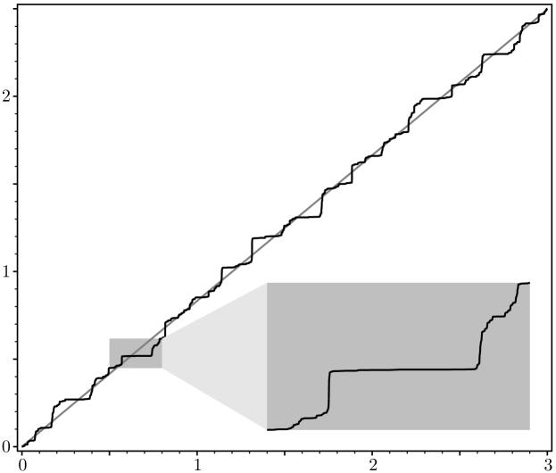
Figure 3. Sketch of the distribution function $F$ from Eq. (7.3) for the singular continuous diffraction measure in the balanced weight case of Eq. (7.1). The straight line is the average slope of $F$, which is $\eta_{0}(0)$ of Eq. (7.2). The enlarged detail is meant to illustrate that $F$ is strictly increasing, which implies that there are no proper plateaux.

Remark 7.1.

On average, the distribution function $F(x)$ grows linearly in $x$, with slope $\eta_{0}(0)$, as also indicated in Figure 3. Furthermore, $F$ is a continuous function that appears to be strictly increasing, in line with the general expectation that the supporting set of such measures must be dense; compare [3, Sec. 10.1]. $\Diamond$

7.2. Outlook

Our main result concerns the absence of absolutely continuous components in the diffraction measure, for arbitrary complex weights. Now, one would like to also infer the absence of absolutely continuous spectral measures for the dynamical system. This would follow if one can also show that patch derived factors have no absolutely continuous diffraction components, as an application of [8, Thm. 15 and Cor. 16].

More generally, our analysis can be applied to other binary systems in complete analogy, where the result will be that an irreducible IDA in conjunction with a certain non-uniform hyperbolic structure in the matrix iterations is incompatible with the presence of absolutely continuous diffraction components. Cases with reducible IDAs can also be handled by explicit methods [29]. The situation for primitive inflation rules over larger alphabets, or for inflation tilings in higher dimensions, is more complex, and will be considered separately.

8. Appendix A: Details of the inward iteration

Here, we study the iteration according to Eq. (6.12) in more detail, where it suffices to consider $k\geqslant 0$. First, choose $c_{\hskip 0.5pt0}>0$ such that $\lvert z(k)\rvert\leqslant 9\hskip 0.5ptc_{\hskip 0.5pt0}k$ for all $k\in\bigl{[}0,\frac{1}{3}\bigr{]}$, which is possible because $z$ is analytic, with $z(k)=\mathcal{O}(k)$ for $k\to 0$. Now, set $v^{\hskip 0.5pt\prime}_{n}=(\alpha_{n},\beta_{n})^{t}$ and consider, for some fixed $0<k\leqslant\frac{1}{3}$, the recursion

(8.1) $$v^{\hskip 0.5pt\prime}_{n}\,=\,\frac{\raisebox{-2.0pt}{$1$}}{\raisebox{0.5pt}{$\mbox{\small$\sqrt{\lambda}$}$}}\,\bigl{(}D-z_{n}\hskip 0.5ptN\bigr{)}\hskip 0.5ptv^{\hskip 0.5pt\prime}_{n-1}$$

with $z_{n}=z\bigl{(}\frac{k}{\lambda^{n}}\bigr{)}$ for $n\in\mathbb{N}$, with arbitrary start vector $v^{\hskip 0.5pt\prime}_{0}\neq 0$. This means that $(\alpha_{n},\beta_{n})^{t}$ stands for $\bigl{(}\alpha(k/\lambda^{n}),\beta(k/\lambda^{n})\bigr{)}^{t}$ in the previous iteration of Eq. (6.12). Observe next that $\det(D-z_{n}\hskip 0.5ptN)=\det\bigl{(}B(k/\lambda^{n})\bigr{)}\neq 0$ for all $n\in\mathbb{N}$ under our condition on $k$, wherefore we know that $v^{\hskip 0.5pt\prime}_{n}\neq 0$ for all $n\geqslant 0$. Also, we have $\lvert z_{n}\rvert\leqslant 9\hskip 0.5ptc_{\hskip 0.5pt0}k\hskip 0.5pt\lambda^{-n}\leqslant 3\hskip 0.5ptc_{\hskip 0.5pt0}\lambda^{-n}$ for all $n\in\mathbb{N}$. Now, with $\|D\|_{\infty}=\lambda$ and $\|N\|_{\infty}=\lambda/3$, we can estimate

$$\|v^{\hskip 0.5pt\prime}_{n}\|_{\infty}\,\leqslant\,\sqrt{\lambda}\,\bigl{(}1+c_{\hskip 0.5pt0}\lambda^{-n}\bigr{)}\|v^{\hskip 0.5pt\prime}_{n-1}\|_{\infty}\leqslant\dots\leqslant\lambda^{n/2}\bigl{(}1+c_{\hskip 0.5pt0}\lambda^{-n}\bigr{)}\cdot\ldots\cdot\bigl{(}1+c_{\hskip 0.5pt0}\lambda^{-1}\bigr{)}\|v^{\hskip 0.5pt\prime}_{0}\|_{\infty}\hskip 0.5pt,$$

which implies $\|v^{\hskip 0.5pt\prime}_{n}\|_{\infty}=\mathcal{O}(\lambda^{n/2})$ because the product $\prod_{m\geqslant 1}\bigl{(}1+c_{\hskip 0.5pt0}\lambda^{-m}\bigr{)}$ is absolutely convergent. Since $\lvert\alpha_{n}\rvert\leqslant\|v^{\hskip 0.5pt\prime}_{n}\|_{\infty}$, this also means

$$\alpha_{n}\,=\,\mathcal{O}(\lambda^{n/2})\quad\text{as $n\to\infty$}\hskip 0.5pt,$$

as well as $\|v^{\hskip 0.5pt\prime}_{n}\|_{\infty}\leqslant c^{\hskip 0.5pt\hskip 0.5pt\prime}\lambda^{n/2}$ for some $c^{\hskip 0.5pt\hskip 0.5pt\prime}>0$ and all $n\in\mathbb{N}_{0}$.

Now, choose $\varepsilon>0$ small enough so that $\lvert z_{n}\rvert\leqslant 3\hskip 0.5ptc\hskip 0.5pt\lambda^{-n}$ holds for all $k\in[0,\varepsilon]$ with

(8.2) $$c\,=\,c(\varepsilon)\,<\,\min\big{\{}\lambda-\sqrt{\lambda},1+\sqrt{\lambda}-\lambda\big{\}}\,=\,1+\sqrt{\lambda}-\lambda\,\approx\,0.2147\hskip 0.5pt,$$

which is clearly possible because $c=3\hskip 0.5ptc_{\hskip 0.5pt0}\varepsilon$. For any $0<k\leqslant\varepsilon$ and $n\in\mathbb{N}_{0}$, we then have

(8.3) $$\Big{\|}\frac{z_{n+1}}{\mbox{\small$\sqrt{\lambda}$}}\,N\hskip 0.5ptv^{\hskip 0.5pt\prime}_{n}\hskip 0.5pt\Big{\|}_{\infty}\hskip 0.5pt\leqslant\,\frac{\raisebox{-2.0pt}{$c\hskip 0.5pt\lambda^{-n}$}}{\raisebox{0.5pt}{$\mbox{\small$\sqrt{\lambda}$}$}}\,\bigl{\|}v^{\hskip 0.5pt\prime}_{n}\bigr{\|}_{\infty}\,\leqslant\,\frac{\raisebox{-2.0pt}{$c$}}{\raisebox{0.5pt}{$\mbox{\small$\sqrt{\lambda}$}$}}\,\bigl{\|}v^{\hskip 0.5pt\prime}_{n}\bigr{\|}_{\infty}\,<\,\frac{\raisebox{-2.0pt}{$\lambda-\mbox{\small$\sqrt{\lambda}$}$}}{\raisebox{0.5pt}{$\mbox{\small$\sqrt{\lambda}$}$}}\,\bigl{\|}v^{\hskip 0.5pt\prime}_{n}\bigr{\|}_{\infty}\hskip 0.5pt.$$

The first estimate, together with Eq. (8.1), implies

$$\lvert\beta_{n+1}\rvert\,\leqslant\,\frac{\raisebox{-2.0pt}{$\lambda-1$}}{\raisebox{0.5pt}{$\mbox{\small$\sqrt{\lambda}$}$}}\,\lvert\beta_{n}\rvert+\frac{\raisebox{-2.0pt}{$c\hskip 0.5pt\lambda^{-n}$}}{\raisebox{0.5pt}{$\mbox{\small$\sqrt{\lambda}$}$}}\,\|v^{\hskip 0.5pt\prime}_{n}\|_{\infty}\,\leqslant\,\frac{\raisebox{-2.0pt}{$\lambda-1$}}{\raisebox{0.5pt}{$\mbox{\small$\sqrt{\lambda}$}$}}\,\lvert\beta_{n}\rvert+\frac{\raisebox{-2.0pt}{$c^{\hskip 0.5pt\hskip 0.5pt\prime\prime}\lambda^{-n/2}$}}{\raisebox{0.5pt}{$\mbox{\small$\sqrt{\lambda}$}$}}$$

with $c^{\hskip 0.5pt\hskip 0.5pt\prime\prime}=c\hskip 0.5ptc^{\hskip 0.5pt\hskip 0.5pt\prime}$. Iterating this estimate inductively gives

$$\begin{split}\lvert\beta_{n+1}\rvert\,&\leqslant\,\frac{(\lambda-1)^{n+1}}{\lambda^{(n+1)/2}}\,\lvert\beta_{0}\rvert+\frac{\raisebox{-2.0pt}{$c^{\hskip 0.5pt\hskip 0.5pt\prime\prime}$}}{\raisebox{0.5pt}{$\lambda^{(n+1)/2}$}}\sum_{m=0}^{n}(\lambda-1)^{m}\\[2.84526pt] &\leqslant\,\lvert\beta_{0}\rvert\,\frac{(\lambda-1)^{n+1}}{\lambda^{(n+1)/2}}+\frac{\raisebox{-2.0pt}{$c^{\hskip 0.5pt\hskip 0.5pt\prime\prime}$}}{\raisebox{0.5pt}{$\lambda-2$}}\,\frac{(\lambda-1)^{n+1}-1}{\lambda^{(n+1)/2}}\\[5.69054pt] &<\,\left(\lvert\beta_{0}\rvert+\frac{\raisebox{-2.0pt}{$c^{\hskip 0.5pt\hskip 0.5pt\prime\prime}$}}{\raisebox{0.5pt}{$\lambda-2$}}\right)\left(\frac{\lambda-1}{\mbox{\small$\sqrt{\lambda}$}}\right)^{\!n+1}\;=\;\mathcal{O}\left(\Bigl{(}\frac{\raisebox{-2.0pt}{$3$}}{\raisebox{0.5pt}{$\lambda^{3/2}$}}\Bigr{)}^{\!n+1}\hskip 0.5pt\right),\end{split}$$

where $(\lambda-1)/\mbox{\small$\sqrt{\lambda}$}=3/\lambda^{3/2}\approx 0.8585<1$. Consequently, we have $\lim_{n\to\infty}\beta_{n}=0$, for any start vector $v_{0}$ and any $0<k\leqslant\varepsilon$.

If $\lvert\alpha_{n}\rvert>\lvert\beta_{n}\rvert$ for some $n$, which is a situation that can already occur for $v^{\hskip 0.5pt\prime}_{0}$, we have $\|v^{\hskip 0.5pt\prime}_{n}\|_{\infty}=\lvert\alpha_{n}\rvert>0$, and the iteration (8.1) with the estimates from Eqs. (8.2) and (8.3) result in

$$\lvert\alpha_{n+1}\rvert\,\geqslant\lvert\alpha_{n}\rvert\,\frac{\raisebox{-2.0pt}{$\lambda-c$}}{\raisebox{0.5pt}{$\mbox{\small$\sqrt{\lambda}$}$}}\,>\,\lvert\alpha_{n}\rvert\quad\text{and}\quad\lvert\beta_{n+1}\rvert\,\leqslant\frac{\raisebox{-2.0pt}{$\lambda-1$}}{\raisebox{0.5pt}{$\mbox{\small$\sqrt{\lambda}$}$}}\,\lvert\beta_{n}\rvert+\frac{\raisebox{-2.0pt}{$c$}}{\raisebox{0.5pt}{$\mbox{\small$\sqrt{\lambda}$}$}}\,\lvert\alpha_{n}\rvert\,<\,\lvert\alpha_{n}\rvert\hskip 0.5pt,$$

so that $\lvert\alpha_{n+1}\rvert>\lvert\beta_{n+1}\rvert$. By induction, $\lvert\alpha_{m+1}\rvert>\lvert\alpha_{m}\rvert>0$ for all $m\geqslant n$, while $\beta_{m}$ goes to $0$ as before. Using the first inequality in Eq. (8.3), we get $\lvert\alpha_{n+1}\rvert\geqslant\mbox{\small$\sqrt{\lambda}$}\,\lvert\alpha_{n}\rvert\hskip 0.5pt\bigl{(}1-c\hskip 0.5pt\lambda^{-n-1}\bigr{)}>0$ and hence, for any $m\in\mathbb{N}$,

$$\lvert\alpha_{n+m}\rvert\,\geqslant\,\lambda^{m/2}\,\lvert\alpha_{n}\rvert\,\prod_{\ell=1}^{m}\bigl{(}1-c\hskip 0.5pt\lambda^{-n-\ell}\bigr{)}.$$

Since the product converges absolutely as $m\to\infty$, we may conclude that $\lvert\alpha_{m}\rvert\geqslant c_{\alpha}\hskip 0.5pt\lambda^{m/2}$ for all $m\geqslant n$, with some constant $c_{\alpha}>0$ that depends on $k$ and $v^{\hskip 0.5pt\prime}_{0}$. With our previous estimate, we thus have $\|v^{\hskip 0.5pt\prime}_{n}\|_{\infty}=\lvert\alpha_{n}\rvert\asymp\lambda^{n/2}$, which means that $\lvert\alpha_{n}\rvert$ is bounded from above and from below by different (positive) multiples of the same exponential function. For any initial vector $v^{\hskip 0.5pt\prime}_{0}$ with this behaviour, we thus obtain the Lyapunov exponent

(8.4) $$\chi_{-}(v^{\hskip 0.5pt\prime}_{0})\,:=\,\limsup_{n\to\infty}\frac{\raisebox{-2.0pt}{$1$}}{\raisebox{0.5pt}{$n$}}\hskip 0.5pt\log\|v^{\hskip 0.5pt\prime}_{n}\|_{\infty}\,=\,\lim_{n\to\infty}\frac{\raisebox{-2.0pt}{$1$}}{\raisebox{0.5pt}{$n$}}\hskip 0.5pt\log\|v^{\hskip 0.5pt\prime}_{n}\|_{\infty}\,=\,\log\mbox{\small$\sqrt{\lambda}$}\,\approx\,0.834\hskip 0.5pt,$$

where the existence of the limit is a simple consequence of the asymptotic behaviour.

It remains to consider the case that $\lvert\alpha_{n}\rvert\leqslant\lvert\beta_{n}\rvert$ for all $n\in\mathbb{N}_{0}$, which implies $\|v^{\hskip 0.5pt\prime}_{n}\|_{\infty}=\lvert\beta_{n}\lvert$. If $\alpha_{n}=0$ for some $n$, we get $\alpha_{n+1}\neq 0$ from the structure of $N$, and hence also $\beta_{n+1}\neq 0$. Note that this is just the irreducibility of $\mathcal{B}$ in action; compare Lemma 5.1. Choose an $n\in\mathbb{N}_{0}$ such that $\beta_{n}\neq 0$ and observe that we then get

$$0\,<\,\lvert\beta_{n}\rvert\,\frac{\raisebox{-2.0pt}{$\lambda-1$}}{\raisebox{0.5pt}{$\mbox{\small$\sqrt{\lambda}$}$}}\,\Bigl{(}1-\frac{\raisebox{-2.0pt}{$c$}}{\raisebox{0.5pt}{$\lambda-1$}}\,\lambda^{-n}\Bigr{)}\,\leqslant\,\lvert\beta_{n+1}\rvert\,\leqslant\,\lvert\beta_{n}\rvert\,\frac{\raisebox{-2.0pt}{$\lambda-1$}}{\raisebox{0.5pt}{$\mbox{\small$\sqrt{\lambda}$}$}}\,\Bigl{(}1+\frac{\raisebox{-2.0pt}{$c$}}{\raisebox{0.5pt}{$\lambda-1$}}\,\lambda^{-n}\Bigr{)}$$

because $0<c<\lambda-1$ with the constant $c$ from Eq. (8.2). The upper estimate implies that $\lvert\beta_{n}\rvert$ is ultimately monotonically decreasing. Iterating the lower estimate leads to

$$\lvert\beta_{n+m}\rvert\,\geqslant\,\left(\frac{\raisebox{-2.0pt}{$\lambda-1$}}{\raisebox{0.5pt}{$\mbox{\small$\sqrt{\lambda}$}$}}\right)^{\!m}\lvert\beta_{n}\rvert\,\prod_{\ell=0}^{m-1}\Bigl{(}1-\frac{\raisebox{-2.0pt}{$c$}}{\raisebox{0.5pt}{$\lambda-1$}}\,\lambda^{-n-\ell}\Bigr{)}$$

for all $m\geqslant 1$. Since the product converges absolutely as $m\to\infty$, we may conclude that $\|v^{\hskip 0.5pt\prime}_{n}\|_{\infty}=\lvert\beta_{n}\rvert\asymp\bigl{(}3/\lambda^{3/2}\bigr{)}^{n}$ as $n\to\infty$, hence also $\lim_{n\to\infty}v^{\hskip 0.5pt\prime}_{n}=0$.

Let us look at a consequence of this asymptotic behaviour on the convergence rate of $\alpha_{n}$. Select an $n$ with $\alpha_{n}\neq 0$, which we know to exist. With $\|v^{\hskip 0.5pt\prime}_{n}\|_{\infty}=\lvert\beta_{n}\rvert$, we then find

$$\lvert\alpha_{n+1}\rvert\,\geqslant\,\mbox{\small$\sqrt{\lambda}$}\,\lvert\alpha_{n}\rvert-\frac{\raisebox{-2.0pt}{$c$}}{\raisebox{0.5pt}{$\lambda^{n+1/2}$}}\,\lvert\beta_{n}\rvert\,\geqslant\,\lvert\alpha_{n}\rvert+\bigl{(}\mbox{\small$\sqrt{\lambda}$}-1\bigr{)}\hskip 0.5pt\lvert\alpha_{n}\rvert\,-\,\widetilde{c}\,\Bigl{(}\frac{\raisebox{-2.0pt}{$3$}}{\raisebox{0.5pt}{$\lambda^{5/2}$}}\Bigr{)}^{\!n}$$

for some constant $\widetilde{c}$ that depends on $k$ and $\beta_{0}$. When $\bigl{(}\mbox{\small$\sqrt{\lambda}$}-1\bigr{)}\hskip 0.5pt\lvert\alpha_{n}\rvert\geqslant\widetilde{c}\,\bigl{(}3/\lambda^{5/2}\bigr{)}^{n}$, one gets $\lvert\alpha_{n+1}\rvert\geqslant\lvert\alpha_{n}\rvert>0$ and then, inductively, $\lvert\alpha_{n+m}\rvert\geqslant\lvert\alpha_{n}\rvert>0$ for all $m\in\mathbb{N}$, which contradicts $\lim_{m\to\infty}\alpha_{m}=0$. Consequently, whenever $\alpha_{n}\neq 0$ in our present case, we must have

$$\lvert\alpha_{n}\rvert\,<\,\frac{\raisebox{-2.0pt}{$\widetilde{c}$}}{\raisebox{0.5pt}{$\mbox{\small$\sqrt{\lambda}$}-1$}}\,\Bigl{(}\frac{\raisebox{-2.0pt}{$3$}}{\raisebox{0.5pt}{$\lambda^{5/2}$}}\Bigr{)}^{\!n}$$

which altogether means $\alpha_{n}=\mathcal{O}\bigl{(}3/\lambda^{5n/2}\bigr{)}$, as well as $\lvert\alpha_{n}/\beta_{n}\rvert=\mathcal{O}(\lambda^{-n})$.

The fact that also this somewhat counterintuitive behaviour does indeed occur can be seen as follows. Under our restriction on $k$, we know that the mapping $v^{\hskip 0.5pt\prime}_{0}\mapsto v^{\hskip 0.5pt\prime}_{n}=Q_{n}(k)\hskip 0.5ptv^{\hskip 0.5pt\prime}_{0}$ is invertible. Consequently, it is possible to choose $v^{\hskip 0.5pt\prime}_{0}\in\partial B_{1}(0)$ in such a way that $v^{\hskip 0.5pt\prime}_{n}=c_{n}\hskip 0.5pt(0,1)^{t}$ for some $c_{n}>0$, which is the contracting direction for $M$ in this representation. Let $v^{\hskip 0.5pt\prime}_{0,n}$ be this initial condition, and consider the sequence $\bigl{(}v^{\hskip 0.5pt\prime}_{0,n}\bigr{)}_{n\in\mathbb{N}}$ constructed this way. As it lies within the compact set $\partial B_{1}(0)$, there is a converging subsequence, with limit $v^{\hskip 0.5pt\prime}_{0,\infty}$, say. By construction, this vector spans a one-dimensional subspace $E^{\hskip 0.5pt\prime}_{-}(k)$ of vectors that behave as just derived under the inward iteration. For any $v^{\hskip 0.5pt\prime}_{0}\in E^{\hskip 0.5pt\prime}_{-}(k)$, we thus get

(8.5) $$\chi_{-}(v^{\hskip 0.5pt\prime}_{0})\,=\,\lim_{n\to\infty}\frac{\raisebox{-2.0pt}{$1$}}{\raisebox{0.5pt}{$n$}}\hskip 0.5pt\log\|v^{\hskip 0.5pt\prime}_{n}\|_{\infty}\,=\,\log\frac{\raisebox{-2.0pt}{$\lambda-1$}}{\raisebox{0.5pt}{$\mbox{\small$\sqrt{\lambda}$}$}}\,=\,\log\frac{\raisebox{-2.0pt}{$3$}}{\raisebox{0.5pt}{$\lambda^{3/2}$}}\,\approx\,-0.153\hskip 0.5pt,$$

where the existence of the Lyapunov exponent as a limit follows as in Eq. (8.4).

9. Appendix B: Two simple scaling arguments

Let us briefly explain the idea to use an ‘impossible’ singularity of a locally integrable function to conclude that such a function must vanish, spelled out in a one-dimensional setting for illustration. Here, for $\lambda>1$ fixed, $h\bigl{(}\frac{x}{\lambda}\bigr{)}=\lambda\hskip 0.5pt\hskip 0.5pth(x)$ would be the (scalar) analogue of Eq. (6.4). This implies $h(x)=\mathcal{O}(x^{-1})$ as $x\to 0$, a contradiction to local integrability unless $h=0$. The precise statement is the following.

Lemma 9.1.

Let $h\in L^{1}\bigl{(}[0,1],\mathbb{C}\hskip 0.5pt\bigr{)}$, and assume that, for some fixed $\lambda>1$, one has

$$h\bigl{(}\tfrac{x}{\lambda}\bigr{)}\,=\,\lambda\,h(x)$$

for a.e. $x\in[0,1]$. Then, $h=0$, which means $h(x)=0$ a.e. in $[0,1]$.

Proof.

By assumption, $h$ is certainly integrable on $\bigl{[}\frac{1}{\lambda},1\bigr{]}$. Since

$$h\bigl{(}\tfrac{x}{\lambda^{m}}\bigr{)}\,=\,\lambda^{m}\hskip 0.5pth(x)$$

also holds for all $m\in\mathbb{N}$ and still for a.e. $x\in[0,1]$, one has

$$\int_{1/\lambda^{m+1}}^{1/\lambda^{m}}\lvert h(x)\rvert\,\mathrm{d}x\,=\,\frac{\raisebox{-2.0pt}{$1$}}{\raisebox{0.5pt}{$\lambda^{m}$}}\int_{1/\lambda}^{1}\big{\lvert}h\bigl{(}\tfrac{y}{\lambda^{m}}\bigr{)}\big{\rvert}\,\mathrm{d}y\,=\int_{1/\lambda}^{1}\lvert h(y)\rvert\,\mathrm{d}y\hskip 0.5pt,$$

via a simple transformation of variable ($y=\lambda^{m}\hskip 0.5ptx$), hence

$$\|h\|_{1}\,=\sum_{m\geq 0}\int_{1/\lambda^{m+1}}^{1/\lambda^{m}}\lvert h(x)\rvert\,\mathrm{d}x\,=\sum_{m\geq 0}\int_{1/\lambda}^{1}\lvert h(x)\rvert\,\mathrm{d}x\hskip 0.5pt.$$

Consequently, $\|h\|_{1}<\infty$ implies $\lvert h(x)\rvert=0$ a.e. on $\bigl{[}\frac{1}{\lambda},1\bigr{]}$. The functional equation then gives $\lvert h(x)\rvert=0$ a.e. on $\bigl{[}\frac{1}{\lambda^{m+1}},\frac{1}{\lambda^{m}}\bigr{]}$ for any $m\geq 0$, hence $h=0$ as claimed. ∎

Let us also discuss why a positive, pointwise defined Lyapunov exponent for the asymptotic growth of a density function $g\geqslant 0$ is incompatible with translation boundedness of the measure $g\mu_{\mathrm{L}}$ defined by $g$, where $\mu_{\mathrm{L}}$ denotes Lebesgue measure on $\mathbb{R}\hskip 0.5pt$.

Lemma 9.2.

Let $g\in L^{1}_{\mathrm{loc}}(\mathbb{R}\hskip 0.5pt_{+})$ be a non-negative function and let $\lambda>1$ be fixed. Assume further that $g$ satisfies the relation $g(\lambda x)\geqslant\vartheta(x)\hskip 0.5ptg(x)$ for a.e. $x>0$, where $\vartheta$ is a bounded, measurable function with $\vartheta(x)>1$ and $\vartheta(\lambda x)=\vartheta(x)$ for a.e. $x>0$. Then, the absolutely continuous measure $g\hskip 0.5pt\mu_{\mathrm{L}}$ is translation bounded if and only if $g=0$ in the Lebesgue sense.

Proof.

If $g$ does not vanish almost everywhere, we have $q:=\int_{0}^{a}g(x)\,\mathrm{d}x>0$ for some $a>0$, and $f:=q^{-1}g$ is a probability density on $[0,a]$. By assumption, we have

$$g(\lambda^{m}x)\,\geqslant\,\vartheta(\lambda^{m-1}x)\cdot\ldots\cdot\vartheta(x)\,g(x)\,=\,\vartheta(x)^{m}\hskip 0.5ptg(x)$$

for any (fixed) $m\in\mathbb{N}$ and a.e. $x>0$, by an iterated application of the assumed estimate. Now, via the (clearly existing) moments of $\vartheta$ relative to $f$, we get

$$\begin{split}\int_{0}^{a\lambda^{m}}\!\!g(x)\,\mathrm{d}x\,&=\,\lambda^{m}\int_{0}^{a}g(\lambda^{m}y)\,\mathrm{d}y\,\geqslant\,q\hskip 0.5pt\lambda^{m}\int_{0}^{a}\vartheta(y)^{m}\,f(y)\,\mathrm{d}y\\[5.69054pt] &=\,q\hskip 0.5pt\lambda^{m}\,\mathbb{E}_{f}\bigl{(}\vartheta^{m}\bigr{)}\,\geqslant\,q\hskip 0.5pt\lambda^{m}\bigl{(}\mathbb{E}_{f}(\vartheta)\bigr{)}^{m}\,=\,q\,(\varTheta_{1}\lambda)^{m},\end{split}$$

where the estimate in the second line is a consequence of Jensen’s inequality, while the first moment, $\varTheta_{1}=\mathbb{E}_{f}(\vartheta)$, clearly satisfies $\varTheta_{1}>1$.

This shows that $\int_{0}^{a\lambda^{m}}g(x)\,\mathrm{d}x\not\in\mathcal{O}(\lambda^{m})$ as $m\to\infty$. However, $g\hskip 0.5pt\mu_{\mathrm{L}}$ translation bounded with $g\geqslant 0$ implies

$$\int_{0}^{L}g(x)\,\mathrm{d}x\,=\,\mathcal{O}(L)\quad\text{as }L\to\infty\hskip 0.5pt,$$

which contradicts the previous estimate. Therefore, we must have $g(x)=0$ for a.e. $x>0$ as claimed. ∎

A simple variant, which applies to cases with a.e. constant Lyapunov exponents as in our example, can be stated as follows.

Lemma 9.3.

Let $g\in L^{1}_{\mathrm{loc}}(\mathbb{R}\hskip 0.5pt_{+})$ be a non-negative function and let $\lambda>1$ be fixed. Assume further that there is an interval $[0,a]$ with $a>0$, a constant $\vartheta>1$, and a measurable function $C$ with $C(x)>0$ for a.e. $x\in[0,a]$ such that $g(\lambda^{m}x)\geqslant C(x)\,\vartheta^{m}\hskip 0.5ptg(x)$ holds for a.e. $x\in[0,a]$. Then, the absolutely continuous measure $g\hskip 0.5pt\mu_{\mathrm{L}}$ is translation bounded if and only if $g=0$ on $[0,a]$ in the Lebesgue sense.

Proof.

Assume to the contrary of our claim that $g(x)>0$ for a subset of $[0,a]$ of positive measure. Then,

$$c_{g}\,:=\int_{0}^{a}C(x)\,g(x)\,\mathrm{d}x\,>\,0$$

because the set $\{x\in[0,a]:C(x)=0\text{ or }g(x)=0\}$ is not of full measure in $[0,a]$. Consequently, one has

$$\int_{0}^{a\lambda^{m}}\!g(x)\,\mathrm{d}x\,\geqslant\,\lambda^{m}\hskip 0.5pt\vartheta^{m}\int_{0}^{a}C(x)\,g(x)\,\mathrm{d}x\,=\,c_{g}\,\lambda^{m}\hskip 0.5pt\vartheta^{m}$$

and thus obtains the same type of contradiction as in the proof of Lemma 9.2. So, we must have $g=0$ on $[0,a]$ in the Lebesgue sense as claimed. ∎

References

- [1] Argabright L and Gil de Lamadrid J, Fourier analysis of unbounded measures on locally compact Abelian groups, Memoirs Amer. Math. Soc., no. 145 (1974).
- [2] Baake M and Gähler F, Pair correlations of aperiodic inflation rules via renormalisation: Some interesting examples, Topol. Appl. 205 (2016) 4–27; arXiv:1511.00885.
- [3] Baake M and Grimm U, Aperiodic Order. Vol. 1: A Mathematical Invitation, Cambridge University Press, Cambridge (2013).
- [4] Baake M and Grimm U, Squirals and beyond: Substitution tilings with singular continuous spectrum, Ergodic Th. & Dynam. Syst. 34 (2014) 1077–1102; arXiv:1205.1384.
-
[5]
Baake M and Haynes A,
A measure-theoretic result for approximation by Delone sets,
preprint
arXiv:1702.04839. - [6] Baake M, Haynes A and Lenz D, Averaging almost periodic functions along exponential sequences, to appear in: Aperiodic Order. Vol. 2: Crystallography and Almost Periodicity, Baake M and Grimm U (eds.), Cambridge University Press, Cambridge (2017), in press; arXiv:1704.08120.
- [7] Baake M and Lenz D, Dynamical systems on translation bounded measures: Pure point dynamical and diffraction spectra, Ergodic Th. & Dynam. Syst. 24 (2004) 1867–1893; arXiv:math.DS/0302231.
- [8] Baake M, Lenz D and van Enter A C D, Dynamical versus diffraction spectrum for structures with finite local complexity, Ergodic Th. & Dynam. Syst. 35 (2015) 2017–2043; arXiv:1307.7518.
- [9] Barreira L and Pesin Y, Nonuniform Hyperbolicity, Cambridge University Press, Cambridge (2007).
- [10] Barreira L and Pesin Y, Introduction to Smooth Ergodic Theory, AMS, Providence, RI (2013).
- [11] Bartlett A, Spectral theory of substitutions, Ergodic Th. & Dynam. Syst., in press; arXiv:1410.8106.
- [12] Berlinkov A and Solomyak B, Singular substitutions of constant length, preprint arXiv:1705.00899.
- [13] Berg C and Forst G, Potential Theory on Locally Compact Abelian Groups, Springer, Berlin (1975).
- [14] Bufetov A and Solomyak B, On the modulus of continuity for spectral measures in substitution dynamics, Adv. Math. 260 (2014) 84–129; arXiv:1305.7373.
- [15] Bugeaud Y, Distribution Modulo One and Diophantine Approximation, Cambridge University Press, Cambridge (2012).
- [16] Clark A and Sadun L, When size matters: Subshifts and their related tiling spaces, Ergodic Th. & Dynam. Syst. 23 (2003) 1043–57; arXiv:math.DS/0201152.
- [17] Corduneanu C, Almost Periodic Functions, 2nd English ed., Chelsea, New York (1989).
- [18] Cornfeld I P, Fomin S V, Sinai Ya G, Ergodic Theory, Springer, New York (1982).
- [19] Dekking F M, The spectrum of dynamical systems arising from substitutions of constant length, Z. Wahrscheinlichkeitsth. verw. Geb. 41 (1978) 221–239.
- [20] Fan A-H, Saussol B and Schmeling J, Products of non-stationary random matrices and multiperiodic equations of several scaling factors, Pacific J. Math. 214 (2004) 31–54; arXiv:math.DS/0210347.
- [21] Frank N P, Multi-dimensional constant-length substitution sequences, Topol. Appl. 152 (2005) 44–69.
- [22] Gil de Lamadrid J and Argabright L N, Almost periodic measures, Memoirs Amer. Math. Soc. 85, no. 428 (1990).
- [23] Harman G, Metric Number Theory, Oxford University Press, New York (1998).
- [24] Hartinger J, Kainhofer R F and Tichy R F, Quasi-Monte Carlo algorithms for unbounded, weighted integration problems, J. Complexity 20 (2004) 654–668.
- [25] Hof A, On diffraction by aperiodic structures, Commun. Math. Phys. 169 (1995) 25–43.
- [26] Kamarul Haili H and Nair R, The discrepancy of some real sequences, Math. Scand. 93 (2003) 268–274.
- [27] Kuipers L and Niederreiter H, Uniform Distribution of Sequences, reprint, Dover, New York (2006).
- [28] Lenz D, Continuity of eigenfunctions of uniquely ergodic dynamical systems and intensity of Bragg peaks, Commun. Math. Phys. 287 (2009) 225–258; arXiv:math-ph/0608026.
- [29] Mañibo N, Lyapunov exponents for binary substitutions of constant length, preprint arXiv:1706.00451.
- [30] Moody R V and Strungaru N, Almost periodic measures and their Fourier transforms, to appear in: Aperiodic Order. Vol. 2: Crystallography and Almost Periodicity, Baake M and Grimm U (eds.), Cambridge University Press, Cambridge (2017), in press.
- [31] Queffélec M, Substitution Dynamical Systems – Spectral Analysis, LNM 1294, 2nd ed., Springer, Berlin (2010).
- [32] Reed M and Simon B, Methods of Modern Mathematical Physics I: Functional Analysis, 2nd ed., Academic Press, San Diego, CA (1980).
- [33] Robinson E A, Symbolic dynamics and tilings of , Proc. Sympos. Appl. Math. 60 (2004) 81–119.
- [34] Sobol I M, Calculation of improper integrals using uniformly distributed sequences, Soviet Math. Dokl. 14 (1973) 734–738.
- [35] Solomyak B, Dynamics of self-similar tilings, Ergod. Th. & Dynam. Syst. 17 (1997) 695–738 and 19 (1999) 1685 (Erratum).
- [36] Viana M, Lectures on Lyapunov Exponents, Cambridge University Press, Cambridge (2013).
- [37] Vince A, Digit tiling of Euclidean space, in: Directions in Mathematical Quasicrystals, Baake M and Moody R V (eds.), CRM Monograph Series vol. 13, AMS, Providence, RI (2000), pp. 329–370.