LMC Blue Supergiant Stars and the Calibration of the Flux-weighted Gravity–Luminosity Relationship.

Abstract

High quality spectra of 90 blue supergiant stars in the Large Magellanic Cloud are analyzed with respect to effective temperature, gravity, metallicity, reddening, extinction and extinction law. An average metallicity, based on Fe and Mg abundances, relative to the Sun of [Z] = -0.35$\pm$0.09 dex is obtained. The reddening distribution peaks at E(B-V) = 0.08 mag, but significantly larger values are also encountered. A wide distribution of the ratio of extinction to reddening is found ranging from R${}_{\!\mbox{\scriptsize\,\sc v}}$= 2 to 6. The results are used to investigate the blue supergiant relationship between flux-weighted gravity, $g_{\!\mbox{\scriptsize\,\sc f}}$$\equiv$ g/$T_{\!\mbox{\scriptsize\em eff}}^{4}$, and absolute bolometric magnitude M_bol. The existence of a tight relationship, the FGLR, is confirmed. However, in contrast to previous work the observations reveal that the FGLR is divided into two parts with a different slope. For flux-weighted gravities larger than 1.30 dex the slope is similar as found in previous work, but the relationship becomes significantly steeper for smaller values of the flux-weighted gravity. A new calibration of the FGLR for extragalactic distance determinations is provided.

s

1 Introduction

Blue supergiants of spectral type A and B are the brightest stars in the universe with absolute visual magnitudes up to $M_{V}\simeq-9.5$ mag. They have long been recognized as potentially valuable distance indicators in external galaxies (Hubble, 1936; Petrie, 1965; Crampton, 1979; Tully & Wolff, 1984; Hill et al., 1986; Humphreys, 1988). With the advent of very large telescopes of the 8 to 10m class equipped with efficient multi-object spectrographs and with the improvements of non-LTE model atmosphere techniques it has become possible to obtain high signal-to-noise spectra of individual supergiant stars in galaxies beyond the Local Group and to quantitatively analyze these spectra to determine stellar parameters such as effective temperature $T_{\!\mbox{\tiny\em eff}}$, gravity $\log\,g$ and metallicity with unprecedented accuracy and reliability. This work has led to the detection of a tight relationship between stellar absolute bolometric magnitude M_bol and the “flux-weighted gravity” $g_{\!\mbox{\scriptsize\,\sc f}}$$\equiv$ g/$T_{\!\mbox{\scriptsize\em eff}}^{4}$ ($T_{\!\mbox{\tiny\em eff}}$ in units of 10⁴K) of the form

$$M_{\rm bol}\,=\,a(\mbox{$\log\,g_{\!\mbox{\scriptsize\,\sc f}}$}\,-\,1.5)\,+\,b,$$ (1)

the “Flux-weighted Gravity - Luminosity Relationship (FGLR)” (see Kudritzki et al., 2003) .

The simple form of the FGLR can be well understood as the result of massive star evolution from the main sequence to the red supergiant phase with constant luminosity and constant mass. Under these simplifying assumptions $g/$$T_{\!\mbox{\scriptsize\em eff}}^{4}$ remains constant during the evolution accross the Hertzsprung-Russell Diagram and the FGLR is then the result of a simple relationship between stellar luminosity $L$ and stellar mass $M$, $L\sim M^{x}$, where the exponent $x$ is a constant number of the order of 3 (see Kudritzki et al. 2008, for details). In reality, the luminosity is not exactly constant during the evolution and also the exponent $x$ decreases with increasing stellar mass, but the FGLR still holds, as a recent detailed investigation using state-of-the-art stellar evolution calculations combined with population synthesis has shown (Meynet et al., 2015).

After a first calibration (Kudritzki et al., 2008) the FGLR-technique has turned into a powerful tool to determine distances to a variety of galaxies in the Local Group (WLM – Urbaneja et al. 2008; M  33 – U et al. 2009) and beyond (M 81 – Kudritzki et al. 2012; NGC 3109 – Hosek et al. 2014; NGC 3621 – Kudritzki et al. 2014) with a great potential to map the local universe out to 10 Mpc with present day telescopes and to reach distances of 30 Mpc with the next generation of extremely large telescopes. The advantage of the technique is that it uses a spectroscopic method where the analysis of the spectrum yields the intrinsic stellar energy distribution allowing for an accurate correction of interstellar reddening and extinction, usually a significant source of uncertainty for many other alternative distance determination methods. In addition, since stellar metallicity is also obtained from the spectra, effects of metallicity on the calibration, if existent, could also be accounted for (we note, however, that the recent work by Meynet et al. 2015 indicates that metallicity effects of the FGLR-method are very small).

A potential weakness of the present work applying the FGLR-technique lies in the calibration of the method. Kudritzki et al. (2008) combined blue supergiant observations from eight galaxies, with distances obtained from a variety of other methods, such as cepheids, eclipsing binaries, stellar cluster membership, etc. A much cleaner way (in the absence of accurate distances for Milky Way blue supergiants) for the calibration is to use solely the Large Magellanic Cloud (LMC) and its blue supergiants. After the work by Pietrzynski et al. (2013), who carried out a comprehensive study of late spectral type eclipsing binaries, the distance to the LMC is known with an accuracy of two percent. This provides an excellent basis for a new calibration of the FGLR.

In this paper, we carry out a first step towards such a new calibration. We present new spectroscopic observations of a sample of 32 blue supergiants obtained with the Magellan Echellete spectrograph at the Las Campanas Clay Telescope. Our core sample is complemented with spectra of another 58 LMC supergiant stars collected from other sources. The spectroscopic material is described in section 2, which also contains a discussion of the combined optical, near- and mid-IR photometry used for the FGLR in conjunction with spectroscopy. The spectra and photometry are then analyzed with respect to effective temperature $T_{\!\mbox{\tiny\em eff}}$, gravity $\log\,g$, metallicity, reddening E(B-V), extinction A_V and extinction law characterized by R${}_{\!\mbox{\scriptsize\,\sc v}}$= A_V/E(B-V). The analysis method is introduced in section 3 and the results are presented in section 4. Section 5 finally discusses the observed FGLR of LMC blue supergiants and introduces a new calibration. The paper finishes with the conclusions and important aspects of future work in section 6.

2 Observational data

2.1 Spectroscopic data

Optical spectra of 32 LMC blue supergiant stars were collected during the nights of October 29th and 30th, 2008, and November 10th, 2010, using the Magellan Echellete spectrograph (MagE, Marshall et al., 2008), a medium resolution, cross-dispersed, optical spectrograph on the Clay Telescope at Las Campanas Observatory. We selected the 1 arcsec slit, providing a nominal resolving power of R$\sim$4100. MagE has a plate scale of 0.3 arsec pixel^-1, and it covers a wide spectral range, $\sim$3100-10000 Å.

The conditions during the three nights were good, with excellent seeing in the first and third nights, between 0.6 and 0.8 arcsec, with long spells of 0.6 arcsec. The seeing during the second night was somewhat worse, with a characteristic value of 0.8-0.9 arcsec and some periods slightly above 1.0 arcsec. We secured two to three consecutive exposures for each star, depending on its magnitude, followed by a ThAr lamp, for wavelength calibration purposes. Besides the program objects, spectrophotometric standards were observed several times during the night at different elevations. In all cases, the slit was placed following the parallactic angle. A number of standard calibration images were taken each night, including twilight flats for illumination correction.

This dataset was processed with the MagE Spectral Extractor pipeline (MASE, Bochanski et al., 2009). Before processing the full sample with this pipeline, we convinced ourselves that the contribution by scattered light is at an irrelevant level, at least for the orders considered here (it could be of some importance for the very bluest orders, covering the range 3100–3400 Å, because of the low flux level achieved during the observations). We achieved signal-to-noise ratios in the continuum of at least 200 for all the observed stars. Using the observations of the spectrophotometric standards we also flux calibrated our spectra around the wavelength region of the Balmer discontinuity to measure the Balmer jump (see section 3).

Our primary MagE sample is supplemented with additional data taken with ESO facilities. First, we retrieved from the ESO archive spectra of 29 early OB-type supergiants obtained with the La Silla 2.2m and the FEROS spectrograph (program 074.D-0021(A), PI Evans, data taken December 26, 27, 29, 30, and 31, 2004). These spectra cover the range from 3500 to 9200 Å at a resolution of R = 48000. This dataset was fully processed using the ESO FEROS-DRS pipeline.

Fully reduced spectra of another 14 B-type supergiants in the clusters N11 and NGC 2004, collected in the context of the VLT-FLAMES Survey of Massive Stars (Evans et al., 2006), were already available to us. The spectral range is $\sim 3900-4750$ Å in the blue with a resolution between 20000 to 27500 and $\sim 6300-6700$ Å in the red, at a somewhat lower resolution (R = 16700).

Finally, reduced spectra of another 16 early B-type supergiants in the Tarantula region, observed within the VLT–FLAMES Tarantula survey (Evans et al., 2011) were kindly made available to us by our colleagues Phillip Dufton and Chris Evans. These cover the 3960–5050 Å  region at R$\sim$7000.

Further information on these two last data sets can be found in the aforementioned references. The characteristic SNR of the stars in the FLAMES, FEROS and VFTS samples ranges from 100 to 200, depending on the visual magnitude of the star considered.

In building our sample of supergiants for the FGLR calibration we selected only objects of luminosity class I with effective temperatures lower than 27000K in order to avoid the main sequence phases of stellar evolution, where luminosity and flux-weighted gravity change significantly. Objects, for which the spectral analysis resulted in a higher effective temperature, were dropped from the sample.

2.2 Photometry

Photometric data in multiple bands, from optical to IR, are available in the literature for most of the stars. Regarding the optical bands, because of the brightness of the stars, we mostly rely on early data taken with photometers. Only a handful of stars (the faint end of the sample) lacks this kind of photometric data. For these, we consider the CCD-based photometry (B and V passbands) provided by different works in the literature. The near-IR data were taken from the 2MASS All Sky Catalog of point sources (Skrutskie et al., 2006). For a significant fraction of the sample, Spitzer/IRAC photometry is also available from the Spitzer survey of the Large Magellanic Cloud (Meixner et al., 2006). The full list of targets along with some basic information is given in Tab. 1 through Tab. 4. For completeness, the photometric data used in this work are collected in Appendix 1, Tab. 11 (optical), Tab. 12 (2MASS) and Tab. 13 (Spitzer/IRAC).

The choice of photometric data is mainly driven by the requirement of minimising the possible sources of artificial scatter in the final FGLR. In the case of the optical photometry, a comparison with the APASS survey (Henden et al., 2016) for the 72 stars studied in this work that are available in this survey results in a mean and standard deviation of the difference for V magnitudes of 0.005$\pm$0.05 mag, and of -0.008$\pm$0.025 mag for the B-V colour. Our conclusion from this comparison is that there is no effect that can be observed between the old photometry used in our work and the modern CCD photometry provided by this survey. On the other hand, a comparison for the 60 stars in common with Zaritsky et al. (2004) is less favourable, with mean and standard deviation for the differences of 0.02$\pm$0.14 mag (with a median absolute deviation of 0.11 mag) and -0.02$\pm$0.58 mag (with median absolute deviation 0.13 mag). Given the excellent agreement found with the APASS survey just discussed, these large differences might suggest that the bright stars in this survey could suffer from the same problems as indicated for example in Massey (2002).

Table 1: LMC BA supergiants observed with MagE.

Star	RA (J2000)	Dec (J2000)	V	SpT/LC	Reference
			(mag)
NGC 2004 8	05 30 40.106	-67 16 37.97	12.43	B9 Ia	E06
Sk-65 67	05 34 35.2302	-65 38 52.600	11.44	A2 Ia	tw
Sk-66 50	05 03 08.82368	-66 57 34.8883	10.63	B8 Ia+	F88
Sk-67 19	04 55 21.60684	-67 26 11.2579	11.19	A3 Ia	tw
Sk-67 137	05 29 42.611	-67 20 47.71	11.93	B8 Ia	E06
Sk-67 140	05 29 56.507	-67 27 30.87	12.42	A1 Ia	tw
Sk-67 141	05 30 01.246	-67 14 36.90	12.01	A2 Iab	E06
Sk-67 143	05 30 07.1165	-67 15 43.178	11.46	A0 Ia	tw
Sk-67 155	05 31 12.822	-67 15 07.98	11.60	A3 Iab	E06
Sk-67 157	05 31 27.933	-67 24 44.25	11.95	B9 Ia	E06
Sk-67 170	05 31 52.972	-67 12 15.32	12.48	A1 Iab	E06
Sk-67 171	05 32 00.791	-67 20 23.02	12.04	B8 Ia	E06
Sk-67 201	05 34 22.46749	-67 01 23.5699	9.87	B9 Ia	E06
Sk-67 204	05 34 50.168	-67 21 12.50	10.87	B8 Ia	F88
Sk-69 2A	04 47 33.224	-69 14 32.87	12.47	A3 Iab	tw
Sk-69 24	04 53 59.519	-69 22 42.57	12.52	B9 Ia	A72
Sk-69 39A	04 55 40.447	-69 26 40.98	12.35	A0 Iab	tw
Sk-69 82	05 14 31.566	-69 13 53.39	10.92	B8 Ia	F88
Sk-69 113	05 21 22.399	-69 27 08.07	10.71	A1 Ia	F88
Sk-69 170	05 30 50.07611	-69 31 29.3838	10.34	A0 Ia	tw
Sk-69 299	05 45 16.61696	-68 59 51.9691	10.24	A2 Ia+	tw
Sk-70 45	05 02 17.804	-70 26 56.74	12.53	A0 Iab	S76
Sk-71 14	05 09 38.91592	-71 24 02.2387	10.62	A0 Ia	F88

Note. — References for the spectral classification: tw–this work; A72–Ardeberg et al. (1972); E06–Evans et al. (2006); F88–Fitzpatrick (1988); S76–Stock et al. (1976).

Table 2: LMC OB supergiants (MagE and FLAMES I)

Star	RA (J2000)	Dec (J2000)	V	SpT/LC	Reference
			(mag)
N11 24	04 55 32.931	-66 25 27.90	13.45	B1 Ib	E06
N11 36	04 57 41.015	-66 29 56.54	13.72	B0.5 Ib	E06
N11 54	04 57 18.332	-66 25 59.59	14.10	B1 Ib	E06
NGC 2004 12	05 30 37.491	-67 16 53.57	13.39	B1.5 Iab	E06
NGC 2004 21	05 30 42.043	-67 21 41.58	13.67	B1.5 Ib	E06
NGC 2004 22	05 30 47.362	-67 17 23.40	13.77	B1.5 Ib	E06
Sk-66 1	04 52 19.053	-66 43 53.23	11.61	B1.5 Ia	F88
Sk-66 15	04 55 22.355	-66 28 19.26	12.81	B0.5 Ia	E06
Sk-66 23	04 56 17.555	-66 18 18.96	13.09	B2.5 Iab	E06
Sk-66 26	04 56 20.575	-66 27 13.83	12.91	B1 Ib	E06
Sk-66 27	04 56 23.476	-66 29 52.04	11.82	B3 Ia	E06
Sk-66 36	04 57 08.824	-66 23 25.15	11.35	B2 Ia	E06
Sk-66 37	04 57 22.078	-66 24 27.67	12.98	B0.7 Ib	E06
Sk-66 166	05 36 04.149	-66 13 43.51	11.71	B2.5 Ia	F88
Sk-67 14	04 54 31.8907	-67 15 24.664	11.52	B1.5 Ia	W02
Sk-67 36	05 01 22.590	-67 20 10.02	12.01	B2.5 Ia	F88
Sk-67 133	05 29 21.684	-67 20 11.34	12.59	B2.5 Iab	E06
Sk-67 154	05 31 03.776	-67 21 20.46	12.61	B1.5 Ia	E06
Sk-67 228	05 37 41.012	-67 43 16.56	11.49	B2 Ia	F88
Sk-68 40	05 05 15.203	-68 02 14.15	11.71	B2.5 Ia	F88
Sk-68 92	05 28 16.157	-68 51 45.58	11.71	B1 Ia	F88
Sk-68 171	05 50 22.979	-68 11 24.62	12.01	B0.7 Ia	F91
Sk-69 43	04 56 10.457	-69 15 38.21	11.94	B1 Ia	A72

Note. — References for the spectral classification: A72–Ardeberg et al. (1972); E06–Evans et al. (2006); F88–Fitzpatrick (1988); F91–Fitzpatrick (1991); W02–Walborn et al. (2002).

Table 3: LMC OB supergiants (FEROS)

Star	RA (J2000)	Dec (J2000)	V	SpT/LC	Reference
			(mag)
Sk-66 5	04 53 30.029	-66 55 28.24	10.73	B2.5 Ia	F88
Sk-66 35	04 57 04.440	-66 34 38.45	11.60	BC1 Ia	F88
Sk-66 106	05 29 00.981	-66 38 27.69	11.72	B1.5 Ia	F88
Sk-66 118	05 30 51.912	-66 54 09.12	11.81	B2 Ia	F88
Sk-67 2	04 47 04.44925	-67 06 53.1076	11.26	B1 Ia+	F88
Sk-67 28	04 58 39.23	-67 11 18.7	12.28	B0.7 Ia	F88
Sk-67 78	05 20 19.07797	-67 18 05.6893	11.26	B3 Ia	F88
Sk-67 90	05 23 00.670	-67 11 21.93	11.29	B1 Ia	F88
Sk-67 112	05 26 56.471	-67 39 34.98	11.90	B0.5 Ia	F88
Sk-67 150	05 30 31.690	-67 00 53.41	12.24	B0.7 Ia	F88
Sk-67 169	05 31 51.588	-67 02 22.29	12.18	B1 Ia	W02
Sk-67 172	05 32 07.336	-67 29 13.94	11.88	B2.5 Ia	F88
Sk-67 173	05 32 10.772	-67 40 25.00	12.04	B0 Ia	M95
Sk-67 206	05 34 55.109	-67 02 37.45	12.00	B0.5 Ia	F88
Sk-67 256	05 44 25.036	-67 13 49.61	11.90	B1 Ia	F88
Sk-68 26	05 01 32.239	-68 10 42.92	11.63	BC2 Ia	F88
Sk-68 41	05 05 27.131	-68 10 02.61	12.01	B0.5 Ia	F87
Sk-68 45	05 06 07.295	-68 07 06.11	12.03	B0 Ia	F88
Sk-68 111	05 31 00.842	-68 53 57.17	12.01	B0.5 Ia	M10
Sk-69 89	05 17 17.5791	-69 46 44.165	11.39	B2.5 Ia	F88
Sk-69 214	05 36 16.436	-69 31 27.09	12.19	B0.7 Ia	F88
Sk-69 228	05 37 09.218	-69 20 19.54	12.12	BC1.5 Ia	F88
Sk-69 237	05 38 01.3126	-69 22 14.079	12.08	B1 Ia	F88
Sk-69 270	05 41 20.408	-69 05 07.36	11.27	B2.5 Ia	F88
Sk-69 274	05 41 27.679	-69 48 03.70	11.21	B2.5 Ia	F88
Sk-70 78	05 06 16.035	-70 29 35.76	11.29	B0.7 Ia	F88
Sk-70 111	05 41 36.790	-70 00 52.65	11.85	B0.5 Ia	F88
Sk-70 120	05 51 20.78027	-70 17 09.3281	11.59	B1 Ia	F88
Sk-71 42	05 30 47.77615	-71 04 02.2976	11.17	B2 Ia	F91

Note. — References for the spectral classification: F87–Fitzpatrick (1987); F88–Fitzpatrick (1988); F91–Fitzpatrick (1991); M95–Massey et al. (1995); M10–Massey (2010); W02–Walborn et al. (2002).

Table 4: LMC VFTS OB Supergiants

Star	RA (J2000)	Dec (J2000)	V	SpT/LC
			(mag)
VFTS 3	05 36 55.17	-69 11 37.7	11.59	B1 Ia+
VFTS 28	05 37 17.856	-69 09 46.23	13.40	B0.7 Ia Nwk
VFTS 69	05 37 33.76	-69 08 13.2	13.59	B0.7 Ib-Iab
VFTS 82	05 37 36.082	-69 06 44.90	13.61	B0.5 Ib-Iab
VFTS 232	05 38 04.774	-69 09 05.53	14.52	B3 Ia
VFTS 270	05 38 15.140	-69 04 01.18	14.35	B3 Ib
VFTS 302	05 38 19.003	-69 11 12.80	15.53	B1.5 Ib
VFTS 315	05 38 20.600	-69 15 37.88	14.81	B1 Ib
VFTS 431	05 38 36.971	-69 05 07.75	12.05	B1.5 Ia Nstr
VFTS 533	05 38 42.742	-69 05 42.44	11.82	B1.5 Ia+p Nwk
VFTS 590	05 38 45.5859	-69 05 47.772	12.49	B0.7 Iab
VFTS 696	05 38 57.18	-68 56 53.1	12.74	B0.7 Ib-Iab Nwk
VFTS 732	05 39 04.777	-69 04 09.96	13.00	B1.5 Iap Nwk
VFTS 831	05 39 39.870	-69 12 04.34	13.04	B5 Ia
VFTS 867	05 40 01.325	-69 07 59.60	14.63	B1 Ib Nwk

Note. — Reference for the spectral classification: McEvoy et al. (2015)

3 Spectral Analysis

As in our previous works (see for example Kudritzki et al., 2008, 2012), the stars are separated in two groups, according to their spectral types. We use the term OB supergiants for stars of Ib to Ia⁺ luminosity classes with spectral types B5 or earlier (note that the earliest star in our sample is of spectral type B0.5 so no O-type supergiants are included), whilst the BA supergiants group is comprised of stars with spectral type B8–A5. For each group, we utilized a different set of model atmosphere and line formation codes suitable for the physical conditions in the atmospheres of these objects. The next two subsections describe the codes employed for the two different groups and a third subsection summarises the methodology of the spectral analysis.

3.1 OB supergiants

For the B0–B5 range we use the model atmosphere/line formation code fastwind (Puls et al., 2005). fastwind includes the effects of stellar winds which are important for the atmospheres of these objects. It solves the radiative transfer problem in the co-moving frame of the expanding atmosphere of an early type star, for a spherically symmetric geometry, considering the constraints of statistical equilibrium and energy conservation, along with chemical homogeneity and steady state. The density stratification is set by the velocity field (pseudo static photosphere plus a wind following a $\beta$-law) via the equation of continuity. A smooth transition between the photosphere, described by a depth-dependent pressure scale-height, and the wind is enforced (see Santolaya-Rey et al., 1997).

Each model is then specified by a set of parameters: effective temperature, surface gravity and stellar radius (all defined at Rosseland optical depth $\tau_{\!\mbox{\scriptsize\,\sc r}}$ $=2/3$), the $\beta$ exponent of the wind-velocity law, the steady mass-loss rate, the wind terminal velocity, the micro-turbulence velocity, and the chemical abundances. In order to reduce the number of parameters to be explored with the model grid, we follow the ideas presented in Urbaneja et al. (2005), with the exception being a fixed micro-turbulence velocity for the calculation of the atmospheric structure. The reader is referred to this last reference for specific information on the model atoms used in our calculations.

The grid of fastwind models utilised in this work explores a total of 10 parameters: effective temperature ($T_{\!\mbox{\tiny\em eff}}$), surface gravity ($\log\,g$), micro-turbulence ($\xi$, fixed to 10 $km\,s^{-1}$ for the calculation of the atmospheric density and temperature stratification but variable for the formal solution), the outflow velocity field parameter $\beta$, an optical depth invariant parameter $Q\,=\dot{M}\left(R_{\star}\,v_{\infty}\right)^{-2/3}$ that characterizes the strength of the wind (assumed to be homogeneous, see Urbaneja et al., 2011), and the abundances of He, C, N, O, Mg and Si. For all other species, we assume the solar abundance pattern scaled down to 0.4 Z_⊙. We adopt a scaling relation between the wind terminal velocity and the escape velocity as prescribed by Kudritzki & Puls (2000).

3.2 BA supergiants

In the case of BA supergiants, we follow closely the procedures introduced by Przybilla et al. (2006). Since the effects of stellar winds are less important in the photospheres of these objects, the atmospheric structure is provided by plane-parallel, hydrostatic model atmospheres calculated assuming local thermodynamic equilibrium (LTE) with the ATLAS9 code (Kurucz, 1993), whilst the occupation numbers and line formation calculation are performed with the DETAIL/SURFACE codes (Giddings, 1981; Buttker & Giddings, 1985), assuming either LTE or non-LTE depending on the species. For the analyses presented in the present work, we consider a model grid defined by a set of 6 parameters for each model: $T_{\!\mbox{\tiny\em eff}}$, $\log\,g$, $\xi$, and the abundances of He, Mg and Fe (all these 3 species, plus H, are treated in non-LTE in all cases). The reader is referred to Przybilla et al. (2006) for details on the applicability limits, and the model atoms used in the non- LTE calculations.

3.3 Methodology

The quantitative spectroscopic analysis of B- and A-type supergiants is well established and the methods have been carefully tested. The reader is referred to the papers cited in the previous paragraphs for a detailed description. Briefly, the combined diagnostic information of ionisation equilibria (Si ii/iii/iv supplemented by He i/ii for OB stars; Mg i/ii and Fe i/ii in the case of BA stars) and of the higher Balmer lines (starting usually at H$\gamma$) are used to determine the fundamental atmospheric parameters (effective temperature, gravity, helium abundance, microturbulence, metal abundances), requiring at the same time that any line is well reproduced. In the case of OB supergiants we additionally utilise H$\alpha$ and H$\beta$ to constrain the strengths and influence of stellar winds, i.e. the $\beta$ and Q parameters.

The methodology just described can be implemented in different ways. In our case, a simultaneous solution for all the relevant parameters is found through a procedure that minimizes the differences between the observation and the model. For each group (OB or BA), a set of key diagnostic lines is defined. The model that minimizes the residuals in these lines then defines the parameters and abundances of the observed star. Tab. 5 shows the set of lines that we have considered for this procedure. We note that all the metal lines used are fairly isolated (unblended) at the spectral resolution of our observational dataset.

Table 5: Diagnostic lines used for the spectral analysis.

Species	Lines
OB Supergiants
H	H$\alpha$, H$\beta$, H$\gamma$, H$\delta$, H$\zeta$
He	He i 4026, 4387, 4713, 4922, 5015, 5876
	He ii 4541, 5411
Mg	Mg ii 4481
Si	Si ii 4128, 4130
	Si iii 4553, 4567, 4574, 5740
	Si iv 4116
BA Supergiants
H	H$\gamma$, H$\delta$, H$\zeta$, H$\eta$
He	He i 5876, 6678
Mg	Mg i 5172, 5183
	Mg ii 4390, 4481
Fe	Fe i 3859, 4045, 4063, 4404
	Fe ii 4233, 4303, 4490, 4505, 4554, 4576
	Fe ii 4731, 5325, 6145, 6416

In the case of BA stars, an extra powerful constraint on $T_{\!\mbox{\tiny\em eff}}$ is provided by the Balmer jump, complementing and sometimes substituting the use of ionisation equilibria, IE (see for example Kudritzki et al., 2008). We have conducted separate analyses, considering on the one hand an IE and the Balmer jump on another, of those stars in the BA group for which we could achieve a reliable flux calibration (only stars observed during our 2008 run, the 2010 data turned out to be of insufficient quality in the region of the Balmer jump for a reliable flux calibration), in order to evaluate the consistency between both $T_{\!\mbox{\tiny\em eff}}$-indicators. This will be discussed in the coming sections.

4 Results

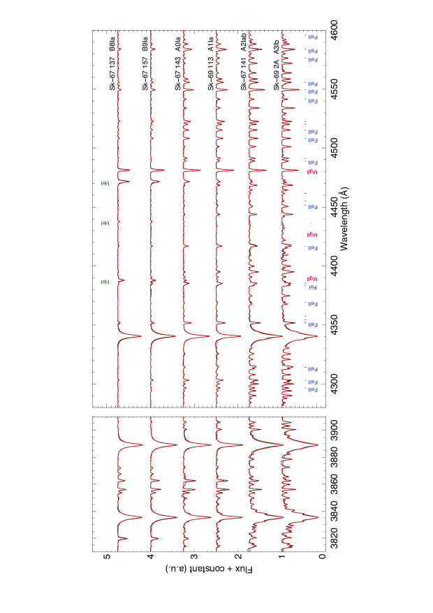
Figure 1: Example fits for some BA supergiants of our sample as a function of spectral type. Iron lines, as well as some other prominent features, are identified.

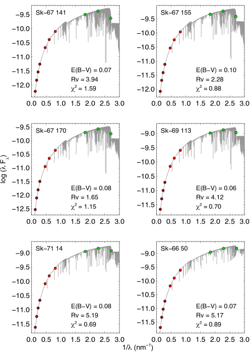
Figure 3: Spectral energy distributions of some BA supergiant stars in our sample. Photometric measurements (filled circles) correspond to Johnson (U, B and V –green circles), 2MASS (J, H, and Ks – light-red circles) and IRAC (3.6, 4.5, 5.8 and 8.0 microns channels – dark-red circles) measurements. Whilst this figure, and the following one, are shown in flux units for illustration purposes, the derivation of E(B-V) and R${}_{\!\mbox{\scriptsize\,\sc v}}$ is based on colours. The reader is referred to the text for a detailed explanation.

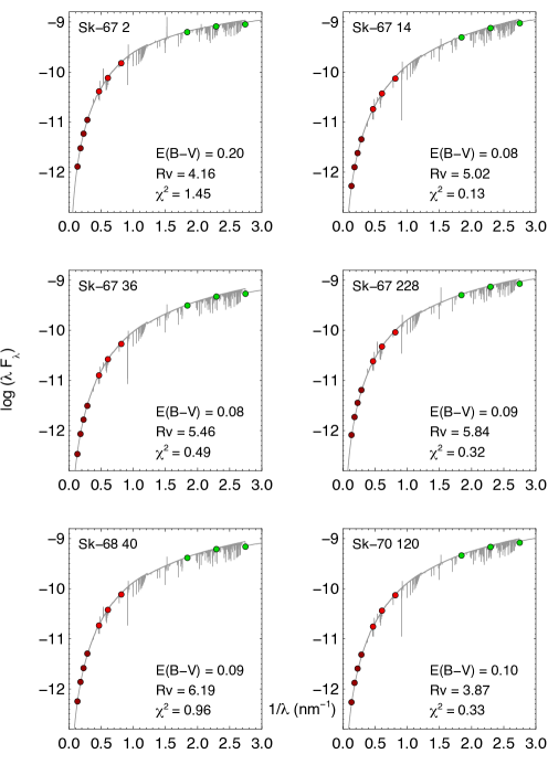
Figure 4: Energy distribution fit of some OB supergiants in the sample. Photometric measurements are in Johnson (U, B and V– green circles), 2MASS (J, H, and Ks – light-red circles) and IRAC (3.6, 4.5, 5.8 and 8.0 microns channels – dark-red circles) measurements. See comments in the caption of the previous figure.

The results of the analysis of our spectra are summarized in Tables 6, 7,  8 and  9. Fig. 1 and 2 give an impression of the quality of the fits and demonstrate that the model spectra calculated with the final parameters of our target stars reproduce the observed spectra very well. Fig. 3 and Fig. 4 show example fits of the observed energy distributions, which are used to determine E(B-V), A_V and R${}_{\!\mbox{\scriptsize\,\sc v}}$ (see subsection 4.4). Note that while we display monochromatic fluxes in these figures for a better illustration of the results, the determination of the reddening parameters is based on filter integrated colours (see below). In the following, we discuss details of our results with respect to stellar evolution (§4.1), metallicity (§4.2), low resolution spectroscopy as applied in the case of extragalactic studies beyond the Local Group (§4.3), and reddening, extinction and extinction law (§4.4).

Table 6: LMC BA supergiants results.

Star	$T_{\!\mbox{\tiny\em eff}}$	$\log\,g_{\!\mbox{\scriptsize\,\sc f}}$	Mg	Fe	BC	E(B-V)	Rv	Av	$\chi^{2}$
	($\times 10^{4}$ K)	(dex)	(dex)	(dex)	(mag)	(mag)		mag
NGC 2004 8	1.1485${}^{+0.0300}_{-0.0275}$	1.69${}^{+0.05}_{-0.06}$	7.39${}^{+0.20}_{-0.13}$	7.06${}^{+0.14}_{-0.16}$	-0.59$\pm$0.04	0.06${}^{+0.02}_{-0.03}$	6.02${}^{+1.88}_{-2.27}$	0.36${}^{+0.03}_{-0.03}$	0.97
Sk-65 67	0.9440${}^{+0.0050}_{-0.0050}$	1.57${}^{+0.02}_{-0.01}$	7.26${}^{+0.18}_{-0.18}$	7.05${}^{+0.13}_{-0.14}$	-0.21$\pm$0.02	0.06${}^{+0.02}_{-0.03}$	4.50${}^{+1.69}_{-2.73}$	0.25${}^{+0.03}_{-0.03}$	2.12
Sk-66 50	1.1900${}^{+0.0420}_{-0.0315}$	1.19${}^{+0.02}_{-0.08}$	7.38${}^{+0.21}_{-0.14}$	7.09${}^{+0.18}_{-0.18}$	-0.72$\pm$0.03	0.07${}^{+0.02}_{-0.03}$	5.17${}^{+1.60}_{-2.32}$	0.39${}^{+0.03}_{-0.03}$	1.10
Sk-67 19	0.8860${}^{+0.0075}_{-0.0125}$	1.59${}^{+0.05}_{-0.02}$	7.37${}^{+0.17}_{-0.16}$	7.31${}^{+0.18}_{-0.14}$	-0.10$\pm$0.06	0.14${}^{+0.04}_{-0.04}$	2.83${}^{+0.70}_{-1.16}$	0.40${}^{+0.03}_{-0.03}$	1.76
Sk-67 137	1.2060${}^{+0.0365}_{-0.0390}$	1.53${}^{+0.06}_{-0.07}$	7.41${}^{+0.17}_{-0.11}$	7.06${}^{+0.14}_{-0.17}$	-0.69$\pm$0.05	0.11${}^{+0.03}_{-0.03}$	1.27${}^{+0.46}_{-0.80}$	0.13${}^{+0.04}_{-0.04}$	0.90
Sk-67 140	0.9675${}^{+0.0045}_{-0.0045}$	1.83${}^{+0.02}_{-0.01}$	7.33${}^{+0.17}_{-0.18}$	7.11${}^{+0.12}_{-0.11}$	-0.24$\pm$0.02	0.11${}^{+0.03}_{-0.03}$	3.22${}^{+0.91}_{-1.53}$	0.34${}^{+0.03}_{-0.03}$	1.03
Sk-67 141	0.9040${}^{+0.0045}_{-0.0045}$	1.95${}^{+0.02}_{-0.01}$	7.32${}^{+0.10}_{-0.12}$	7.29${}^{+0.10}_{-0.09}$	-0.12$\pm$0.03	0.07${}^{+0.02}_{-0.03}$	3.94${}^{+1.18}_{-2.02}$	0.29${}^{+0.04}_{-0.04}$	1.45
Sk-67 143	1.0135${}^{+0.0095}_{-0.0090}$	1.51${}^{+0.04}_{-0.02}$	7.37${}^{+0.04}_{-0.07}$	7.28${}^{+0.08}_{-0.05}$	-0.34$\pm$0.04	0.07${}^{+0.03}_{-0.03}$	3.63${}^{+1.36}_{-2.58}$	0.24${}^{+0.03}_{-0.03}$	1.09
Sk-67 155	0.9295${}^{+0.0035}_{-0.0030}$	1.74${}^{+0.02}_{-0.01}$	7.38${}^{+0.15}_{-0.14}$	7.31${}^{+0.10}_{-0.10}$	-0.17$\pm$0.02	0.10${}^{+0.03}_{-0.03}$	2.28${}^{+0.71}_{-1.33}$	0.23${}^{+0.03}_{-0.03}$	1.10
Sk-67 157	1.1420${}^{+0.0205}_{-0.0200}$	1.66${}^{+0.04}_{-0.04}$	7.44${}^{+0.13}_{-0.09}$	7.09${}^{+0.13}_{-0.14}$	-0.58$\pm$0.03	0.07${}^{+0.03}_{-0.03}$	3.65${}^{+1.31}_{-2.41}$	0.27${}^{+0.04}_{-0.03}$	3.04
Sk-67 170	0.9615${}^{+0.0070}_{-0.0055}$	1.89${}^{+0.02}_{-0.02}$	7.30${}^{+0.17}_{-0.19}$	7.14${}^{+0.13}_{-0.14}$	-0.22$\pm$0.02	0.08${}^{+0.03}_{-0.03}$	1.65${}^{+0.69}_{-1.50}$	0.13${}^{+0.04}_{-0.04}$	1.06
Sk-67 171	1.2080${}^{+0.0225}_{-0.0215}$	1.63${}^{+0.04}_{-0.04}$	7.39${}^{+0.20}_{-0.13}$	7.01${}^{+0.11}_{-0.14}$	-0.71$\pm$0.03	0.06${}^{+0.02}_{-0.03}$	4.33${}^{+1.67}_{-2.75}$	0.24${}^{+0.03}_{-0.03}$	1.76
Sk-67 201	1.0120${}^{+0.0090}_{-0.0160}$	1.20${}^{+0.03}_{-0.02}$	7.49${}^{+0.12}_{-0.07}$	7.25${}^{+0.11}_{-0.08}$	-0.36$\pm$0.03	0.06${}^{+0.02}_{-0.03}$	5.36${}^{+1.77}_{-2.48}$	0.33${}^{+0.03}_{-0.03}$	1.03
Sk-67 204	1.0730${}^{+0.0365}_{-0.0400}$	1.26${}^{+0.06}_{-0.07}$	7.36${}^{+0.21}_{-0.14}$	7.06${}^{+0.17}_{-0.17}$	-0.47$\pm$0.05	0.06${}^{+0.02}_{-0.03}$	3.96${}^{+1.52}_{-2.76}$	0.23${}^{+0.03}_{-0.03}$	1.88
Sk-69 2A	0.8465${}^{+0.0045}_{-0.0040}$	1.92${}^{+0.03}_{-0.01}$	7.34${}^{+0.13}_{-0.14}$	7.20${}^{+0.09}_{-0.09}$	-0.01$\pm$0.02	0.22${}^{+0.03}_{-0.03}$	3.31${}^{+0.45}_{-0.57}$	0.71${}^{+0.03}_{-0.03}$	2.37
Sk-69 24	1.0660${}^{+0.0140}_{-0.0155}$	1.77${}^{+0.03}_{-0.03}$	7.42${}^{+0.15}_{-0.11}$	7.14${}^{+0.11}_{-0.11}$	-0.41$\pm$0.03	0.16${}^{+0.03}_{-0.03}$	2.79${}^{+0.58}_{-0.84}$	0.43${}^{+0.03}_{-0.03}$	1.70
Sk-69 39A	0.9140${}^{+0.0055}_{-0.0055}$	1.89${}^{+0.03}_{-0.01}$	7.34${}^{+0.14}_{-0.15}$	7.25${}^{+0.13}_{-0.12}$	-0.13$\pm$0.03	0.13${}^{+0.03}_{-0.03}$	4.13${}^{+0.93}_{-1.50}$	0.54${}^{+0.03}_{-0.03}$	2.22
Sk-69 82	1.0935${}^{+0.0400}_{-0.0440}$	1.24${}^{+0.05}_{-0.07}$	7.35${}^{+0.22}_{-0.15}$	7.06${}^{+0.17}_{-0.18}$	-0.53$\pm$0.05	0.07${}^{+0.02}_{-0.03}$	4.58${}^{+1.49}_{-2.28}$	0.33${}^{+0.03}_{-0.03}$	1.57
Sk-69 113	0.9245${}^{+0.0085}_{-0.0115}$	1.33${}^{+0.03}_{-0.02}$	7.35${}^{+0.14}_{-0.14}$	7.05${}^{+0.10}_{-0.11}$	-0.19$\pm$0.05	0.06${}^{+0.02}_{-0.03}$	4.12${}^{+1.50}_{-2.74}$	0.26${}^{+0.04}_{-0.03}$	1.02
Sk-69 170	1.0140${}^{+0.0105}_{-0.0175}$	1.24${}^{+0.06}_{-0.02}$	7.48${}^{+0.14}_{-0.07}$	7.28${}^{+0.12}_{-0.07}$	-0.33$\pm$0.04	0.12${}^{+0.03}_{-0.03}$	4.42${}^{+1.03}_{-1.61}$	0.53${}^{+0.03}_{-0.03}$	1.10
Sk-69 299	0.8850${}^{+0.0040}_{-0.0040}$	1.24${}^{+0.02}_{-0.01}$	7.39${}^{+0.14}_{-0.14}$	7.19${}^{+0.11}_{-0.11}$	-0.13$\pm$0.02	0.17${}^{+0.03}_{-0.03}$	3.09${}^{+0.58}_{-0.79}$	0.52${}^{+0.03}_{-0.03}$	1.52
Sk-70 45	1.1200${}^{+0.0225}_{-0.0200}$	1.79${}^{+0.03}_{-0.05}$	7.39${}^{+0.17}_{-0.13}$	7.05${}^{+0.12}_{-0.12}$	-0.54$\pm$0.03	0.08${}^{+0.03}_{-0.03}$	2.76${}^{+0.96}_{-1.89}$	0.23${}^{+0.04}_{-0.04}$	1.45
Sk-71 14	0.9900${}^{+0.0045}_{-0.0040}$	1.27${}^{+0.01}_{-0.01}$	7.29${}^{+0.27}_{-0.21}$	7.29${}^{+0.21}_{-0.18}$	-0.33$\pm$0.01	0.08${}^{+0.02}_{-0.03}$	5.19${}^{+1.46}_{-2.27}$	0.43${}^{+0.03}_{-0.03}$	1.01

Note. — The values in the last column correspond to the final reduced-$\chi^{2}$ value resulting in the R${}_{\!\mbox{\scriptsize\,\sc v}}$–E(B-V) analysis.

Table 7: LMC OB supergiants results (MagE and FLAMES I).

Star	$T_{\!\mbox{\tiny\em eff}}$	$\log\,g_{\!\mbox{\scriptsize\,\sc f}}$	Mg	BC	E(B-V)	Rv	Av	$\chi^{2}$
	($\times 10^{4}$ K)	(dex)	(dex)	(mag)	(mag)		(mag)
N11 24	2.3360 ${}^{+0.0285}_{-0.0290}$	1.41 ${}^{+0.03}_{-0.03}$	7.21${}^{+0.10}_{-0.11}$	-2.31$\pm$0.01	0.14${}^{+0.03}_{-0.03}$	4.20${}^{+0.81}_{-1.25}$	0.57${}^{+0.04}_{-0.03}$	1.73
N11 36	2.5450 ${}^{+0.0290}_{-0.0260}$	1.53 ${}^{+0.03}_{-0.03}$	7.17${}^{+0.12}_{-0.12}$	-2.52$\pm$0.01	0.07${}^{+0.01}_{-0.02}$	7.07${}^{+1.75}_{-1.75}$	0.52${}^{+0.04}_{-0.04}$	0.22
N11 54	2.5550 ${}^{+0.0310}_{-0.0290}$	1.52 ${}^{+0.03}_{-0.03}$	7.14${}^{+0.12}_{-0.12}$	-2.52$\pm$0.01	0.14${}^{+0.03}_{-0.03}$	5.89${}^{+1.03}_{-1.44}$	0.85${}^{+0.04}_{-0.04}$	0.77
NGC 2004 12	2.4110 ${}^{+0.0330}_{-0.0315}$	1.52 ${}^{+0.03}_{-0.03}$	7.20${}^{+0.11}_{-0.12}$	-2.40$\pm$0.01	0.03${}^{+0.01}_{-0.02}$	5.20${}^{+2.37}_{-2.82}$	0.13${}^{+0.04}_{-0.04}$	1.02
NGC 2004 21	2.3620 ${}^{+0.0320}_{-0.0310}$	1.63 ${}^{+0.02}_{-0.02}$	7.18${}^{+0.12}_{-0.11}$	-2.29$\pm$0.01	0.05${}^{+0.02}_{-0.03}$	3.38${}^{+1.57}_{-2.98}$	0.16${}^{+0.05}_{-0.05}$	0.50
NGC 2004 22	2.3880 ${}^{+0.0300}_{-0.0310}$	1.69 ${}^{+0.03}_{-0.03}$	7.09${}^{+0.10}_{-0.11}$	-2.35$\pm$0.01	0.08${}^{+0.01}_{-0.01}$	8.52${}^{+1.42}_{-0.97}$	0.65${}^{+0.05}_{-0.05}$	0.66
Sk-66 1	2.0665 ${}^{+0.0300}_{-0.0250}$	1.18 ${}^{+0.01}_{-0.01}$	7.28${}^{+0.06}_{-0.07}$	-1.98$\pm$0.01	0.09${}^{+0.02}_{-0.03}$	5.99${}^{+1.41}_{-1.93}$	0.57${}^{+0.03}_{-0.03}$	0.25
Sk-66 15	2.6065 ${}^{+0.0255}_{-0.0270}$	1.28 ${}^{+0.03}_{-0.03}$	7.14${}^{+0.12}_{-0.13}$	-2.59$\pm$0.01	0.08${}^{+0.02}_{-0.03}$	5.79${}^{+1.50}_{-2.04}$	0.49${}^{+0.03}_{-0.03}$	1.21
Sk-66 23	1.9700 ${}^{+0.0315}_{-0.0310}$	1.37 ${}^{+0.02}_{-0.02}$	7.15${}^{+0.09}_{-0.10}$	-1.86$\pm$0.01	0.23${}^{+0.03}_{-0.03}$	4.41${}^{+0.53}_{-0.70}$	1.02${}^{+0.04}_{-0.04}$	0.70
Sk-66 26	2.3085 ${}^{+0.0390}_{-0.0350}$	1.32 ${}^{+0.02}_{-0.02}$	7.07${}^{+0.08}_{-0.08}$	-2.23$\pm$0.01	0.13${}^{+0.03}_{-0.03}$	3.87${}^{+0.83}_{-1.27}$	0.49${}^{+0.04}_{-0.03}$	0.62
Sk-66 27	1.7765 ${}^{+0.0345}_{-0.0300}$	1.24 ${}^{+0.02}_{-0.02}$	7.25${}^{+0.10}_{-0.15}$	-1.62$\pm$0.01	0.15${}^{+0.03}_{-0.03}$	4.82${}^{+0.87}_{-1.23}$	0.71${}^{+0.03}_{-0.03}$	1.32
Sk-66 36	1.9075 ${}^{+0.0325}_{-0.0330}$	1.16 ${}^{+0.02}_{-0.02}$	7.17${}^{+0.09}_{-0.09}$	-1.80$\pm$0.01	0.19${}^{+0.03}_{-0.03}$	4.95${}^{+0.70}_{-0.95}$	0.94${}^{+0.03}_{-0.03}$	1.60
Sk-66 37	2.5400 ${}^{+0.0370}_{-0.0330}$	1.34 ${}^{+0.02}_{-0.02}$	7.05${}^{+0.11}_{-0.13}$	-2.47$\pm$0.01	0.11${}^{+0.02}_{-0.03}$	6.26${}^{+1.35}_{-1.76}$	0.69${}^{+0.03}_{-0.03}$	0.08
Sk-66 166	1.9195 ${}^{+0.0135}_{-0.0120}$	1.21 ${}^{+0.01}_{-0.01}$	7.21${}^{+0.06}_{-0.07}$	-1.87$\pm$0.01	0.10${}^{+0.03}_{-0.03}$	5.41${}^{+1.26}_{-1.89}$	0.55${}^{+0.03}_{-0.04}$	0.76
Sk-67 14	2.2890 ${}^{+0.0120}_{-0.0125}$	1.24 ${}^{+0.01}_{-0.01}$	7.19${}^{+0.10}_{-0.11}$	-2.22$\pm$0.01	0.08${}^{+0.02}_{-0.03}$	5.02${}^{+1.47}_{-2.30}$	0.38${}^{+0.03}_{-0.03}$	0.13
Sk-67 36	1.9395 ${}^{+0.0165}_{-0.0175}$	1.26 ${}^{+0.01}_{-0.01}$	7.26${}^{+0.09}_{-0.10}$	-1.88$\pm$0.01	0.08${}^{+0.02}_{-0.03}$	5.46${}^{+1.55}_{-2.14}$	0.42${}^{+0.04}_{-0.03}$	0.49
Sk-67 133	1.9300 ${}^{+0.0270}_{-0.0280}$	1.46 ${}^{+0.02}_{-0.02}$	7.22${}^{+0.09}_{-0.11}$	-1.87$\pm$0.01	0.11${}^{+0.03}_{-0.03}$	3.80${}^{+0.89}_{-1.52}$	0.40${}^{+0.04}_{-0.03}$	0.42
Sk-67 154	2.3280 ${}^{+0.0300}_{-0.0300}$	1.35 ${}^{+0.03}_{-0.03}$	7.15${}^{+0.11}_{-0.11}$	-2.29$\pm$0.01	0.11${}^{+0.03}_{-0.03}$	1.63${}^{+0.50}_{-0.82}$	0.18${}^{+0.04}_{-0.04}$	0.98
Sk-67 228	2.0465 ${}^{+0.0215}_{-0.0215}$	1.15 ${}^{+0.02}_{-0.02}$	7.21${}^{+0.09}_{-0.08}$	-2.05$\pm$0.01	0.09${}^{+0.02}_{-0.03}$	5.84${}^{+1.47}_{-1.99}$	0.52${}^{+0.03}_{-0.03}$	0.32
Sk-68 40	1.9125 ${}^{+0.0250}_{-0.0230}$	1.25 ${}^{+0.02}_{-0.02}$	7.33${}^{+0.06}_{-0.06}$	-1.84$\pm$0.01	0.08${}^{+0.02}_{-0.03}$	6.19${}^{+1.55}_{-1.98}$	0.53${}^{+0.03}_{-0.03}$	0.96
Sk-68 92	2.2090 ${}^{+0.0210}_{-0.0195}$	1.19 ${}^{+0.02}_{-0.02}$	7.21${}^{+0.08}_{-0.08}$	-2.13$\pm$0.01	0.09${}^{+0.03}_{-0.03}$	4.83${}^{+1.23}_{-1.99}$	0.46${}^{+0.03}_{-0.03}$	0.34
Sk-68 171	2.4405 ${}^{+0.0275}_{-0.0265}$	1.18 ${}^{+0.03}_{-0.03}$	7.31${}^{+0.14}_{-0.14}$	-2.43$\pm$0.01	0.09${}^{+0.03}_{-0.03}$	4.94${}^{+1.31}_{-2.00}$	0.45${}^{+0.04}_{-0.04}$	0.80
Sk-69 43	2.2845 ${}^{+0.0245}_{-0.0220}$	1.18 ${}^{+0.02}_{-0.02}$	7.22${}^{+0.11}_{-0.11}$	-2.25$\pm$0.01	0.10${}^{+0.03}_{-0.03}$	4.33${}^{+1.11}_{-1.81}$	0.42${}^{+0.04}_{-0.04}$	0.48

Note. — The values in the last column correspond to the final reduced-$\chi^{2}$ value resulting in the R${}_{\!\mbox{\scriptsize\,\sc v}}$–E(B-V) analysis.

Table 8: LMC OB supergiants results (FEROS).

Star	$T_{\!\mbox{\tiny\em eff}}$	$\log\,g_{\!\mbox{\scriptsize\,\sc f}}$	Mg	BC	E(B-V)	Rv	Av	$\chi^{2}$
	($\times 10^{4}$ K)	(dex)	(dex)	(mag)	(mag)		(mag)
Sk-66 5	1.7185${}^{+0.0340}_{-0.0310}$	1.10${}^{+0.02}_{-0.02}$	7.16${}^{+0.04}_{-0.08}$	-1.54 $\pm$0.01	0.08${}^{+0.02}_{-0.03}$	4.56${}^{+1.37}_{-2.26}$	0.35${}^{+0.03}_{-0.03}$	0.63
Sk-66 35	2.2000${}^{+0.0320}_{-0.0310}$	1.23${}^{+0.02}_{-0.02}$	7.06${}^{+0.10}_{-0.10}$	-2.20 $\pm$0.01	0.09${}^{+0.02}_{-0.03}$	5.48${}^{+1.39}_{-2.02}$	0.51${}^{+0.03}_{-0.03}$	0.66
Sk-66 106	2.2550${}^{+0.0216}_{-0.0225}$	1.25${}^{+0.03}_{-0.03}$	7.13${}^{+0.10}_{-0.09}$	-2.20 $\pm$0.01	0.09${}^{+0.03}_{-0.03}$	4.78${}^{+1.18}_{-1.92}$	0.45${}^{+0.03}_{-0.04}$	1.88
Sk-66 118	2.1355${}^{+0.0273}_{-0.0170}$	1.25${}^{+0.01}_{-0.01}$	7.21${}^{+0.09}_{-0.07}$	-2.04 $\pm$0.01	0.11${}^{+0.03}_{-0.03}$	3.99${}^{+0.96}_{-1.49}$	0.43${}^{+0.03}_{-0.03}$	0.56
Sk-67 2	1.9910${}^{+0.0358}_{-0.0390}$	1.12${}^{+0.03}_{-0.02}$	7.11${}^{+0.10}_{-0.10}$	-2.00 $\pm$0.01	0.20${}^{+0.03}_{-0.03}$	4.15${}^{+0.58}_{-0.74}$	0.83${}^{+0.03}_{-0.03}$	1.45
Sk-67 28	2.4900${}^{+0.0233}_{-0.0255}$	1.15${}^{+0.02}_{-0.02}$	7.08${}^{+0.12}_{-0.12}$	-2.46 $\pm$0.01	0.05${}^{+0.01}_{-0.02}$	6.10${}^{+1.92}_{-2.25}$	0.33${}^{+0.04}_{-0.04}$	0.36
Sk-67 78	1.6150${}^{+0.0098}_{-0.0175}$	1.20${}^{+0.01}_{-0.02}$	7.28${}^{+0.10}_{-0.05}$	-1.47 $\pm$0.01	0.06${}^{+0.02}_{-0.03}$	4.05${}^{+1.47}_{-2.51}$	0.24${}^{+0.04}_{-0.04}$	1.82
Sk-67 90	2.2240${}^{+0.0200}_{-0.0215}$	1.19${}^{+0.02}_{-0.02}$	6.92${}^{+0.08}_{-0.08}$	-2.16 $\pm$0.01	0.08${}^{+0.02}_{-0.03}$	5.60${}^{+1.56}_{-2.19}$	0.43${}^{+0.03}_{-0.03}$	0.08
Sk-67 112	2.5725${}^{+0.0710}_{-0.0670}$	1.19${}^{+0.05}_{-0.05}$	7.14${}^{+0.23}_{-0.25}$	-2.55 $\pm$0.01	0.06${}^{+0.02}_{-0.03}$	3.25${}^{+1.30}_{-2.44}$	0.19${}^{+0.04}_{-0.04}$	0.51
Sk-67 150	2.3715${}^{+0.0230}_{-0.0245}$	1.16${}^{+0.03}_{-0.03}$	7.35${}^{+0.15}_{-0.17}$	-2.33 $\pm$0.01	0.08${}^{+0.02}_{-0.03}$	5.76${}^{+1.62}_{-2.17}$	0.44${}^{+0.04}_{-0.04}$	1.46
Sk-67 169	2.3660${}^{+0.0260}_{-0.0235}$	1.20${}^{+0.02}_{-0.02}$	6.99${}^{+0.11}_{-0.10}$	-2.30 $\pm$0.01	0.07${}^{+0.02}_{-0.02}$	6.16${}^{+1.72}_{-2.12}$	0.43${}^{+0.03}_{-0.03}$	1.16
Sk-67 172	1.9800${}^{+0.0455}_{-0.0390}$	1.29${}^{+0.02}_{-0.02}$	7.10${}^{+0.08}_{-0.05}$	-1.92 $\pm$0.01	0.09${}^{+0.03}_{-0.03}$	4.81${}^{+1.32}_{-2.12}$	0.41${}^{+0.04}_{-0.03}$	2.15
Sk-67 173	2.7000${}^{+0.0360}_{-0.0345}$	1.20${}^{+0.03}_{-0.03}$	6.99${}^{+0.14}_{-0.16}$	-2.66 $\pm$0.01	0.08${}^{+0.02}_{-0.03}$	5.14${}^{+1.42}_{-2.17}$	0.42${}^{+0.04}_{-0.04}$	1.51
Sk-67 206	2.5230${}^{+0.0235}_{-0.0180}$	1.14${}^{+0.01}_{-0.01}$	7.21${}^{+0.15}_{-0.16}$	-2.50 $\pm$0.01	0.08${}^{+0.03}_{-0.03}$	3.85${}^{+1.13}_{-2.06}$	0.31${}^{+0.03}_{-0.03}$	0.87
Sk-67 256	2.2400${}^{+0.0570}_{-0.0530}$	1.23${}^{+0.04}_{-0.04}$	7.00${}^{+0.14}_{-0.18}$	-2.21 $\pm$0.01	0.10${}^{+0.02}_{-0.03}$	6.15${}^{+1.47}_{-1.91}$	0.59${}^{+0.03}_{-0.03}$	2.43
Sk-68 26	1.8160${}^{+0.0210}_{-0.0200}$	1.15${}^{+0.02}_{-0.02}$	7.09${}^{+0.09}_{-0.09}$	-1.74 $\pm$0.01	0.22${}^{+0.03}_{-0.03}$	4.25${}^{+0.55}_{-0.66}$	0.94${}^{+0.03}_{-0.04}$	0.13
Sk-68 41	2.4970${}^{+0.0350}_{-0.0300}$	1.14${}^{+0.02}_{-0.02}$	7.15${}^{+0.15}_{-0.15}$	-2.48 $\pm$0.01	0.06${}^{+0.01}_{-0.02}$	7.07${}^{+1.91}_{-1.77}$	0.42${}^{+0.03}_{-0.03}$	1.98
Sk-68 45	2.6675${}^{+0.0445}_{-0.0410}$	1.13${}^{+0.02}_{-0.02}$	7.07${}^{+0.14}_{-0.14}$	-2.63 $\pm$0.01	0.07${}^{+0.03}_{-0.03}$	3.75${}^{+1.21}_{-2.21}$	0.27${}^{+0.04}_{-0.04}$	0.36
Sk-68 111	2.3645${}^{+0.0700}_{-0.0700}$	1.25${}^{+0.08}_{-0.09}$	7.07${}^{+0.20}_{-0.27}$	-2.37 $\pm$0.01	0.10${}^{+0.03}_{-0.03}$	3.94${}^{+0.97}_{-1.67}$	0.41${}^{+0.04}_{-0.04}$	2.57
Sk-69 89	1.8255${}^{+0.0222}_{-0.0302}$	1.21${}^{+0.01}_{-0.01}$	7.24${}^{+0.07}_{-0.07}$	-1.70 $\pm$0.01	0.08${}^{+0.02}_{-0.03}$	6.05${}^{+1.59}_{-2.05}$	0.50${}^{+0.03}_{-0.03}$	0.52
Sk-69 214	2.4870${}^{+0.0215}_{-0.0230}$	1.28${}^{+0.03}_{-0.03}$	7.10${}^{+0.11}_{-0.11}$	-2.44 $\pm$0.01	0.19${}^{+0.03}_{-0.03}$	3.92${}^{+0.58}_{-0.76}$	0.75${}^{+0.04}_{-0.04}$	1.36
Sk-69 228	2.0615${}^{+0.0570}_{-0.0405}$	1.22${}^{+0.02}_{-0.02}$	6.97${}^{+0.08}_{-0.08}$	-2.01 $\pm$0.01	0.20${}^{+0.03}_{-0.03}$	3.92${}^{+0.58}_{-0.73}$	0.77${}^{+0.04}_{-0.04}$	0.06
Sk-69 237	2.4625${}^{+0.0430}_{-0.0405}$	1.24${}^{+0.06}_{-0.06}$	7.02${}^{+0.16}_{-0.20}$	-2.41 $\pm$0.01	0.15${}^{+0.03}_{-0.03}$	4.20${}^{+0.76}_{-1.09}$	0.62${}^{+0.03}_{-0.04}$	0.23
Sk-69 270	1.6825${}^{+0.0335}_{-0.0300}$	1.12${}^{+0.02}_{-0.02}$	7.28${}^{+0.09}_{-0.09}$	-1.51 $\pm$0.01	0.22${}^{+0.03}_{-0.03}$	3.84${}^{+0.47}_{-0.61}$	0.87${}^{+0.04}_{-0.04}$	1.01
Sk-69 274	1.8020${}^{+0.0170}_{-0.0180}$	1.17${}^{+0.02}_{-0.02}$	7.43${}^{+0.05}_{-0.04}$	-1.66 $\pm$0.01	0.15${}^{+0.03}_{-0.03}$	4.40${}^{+0.75}_{-1.13}$	0.68${}^{+0.03}_{-0.03}$	2.88
Sk-70 78	2.3430${}^{+0.0415}_{-0.0415}$	1.24${}^{+0.02}_{-0.02}$	7.05${}^{+0.11}_{-0.10}$	-2.29 $\pm$0.01	0.10${}^{+0.03}_{-0.03}$	3.88${}^{+1.02}_{-1.73}$	0.37${}^{+0.03}_{-0.04}$	0.95
Sk-70 111	2.5650${}^{+0.0416}_{-0.0365}$	1.25${}^{+0.02}_{-0.02}$	7.03${}^{+0.11}_{-0.10}$	-2.56 $\pm$0.01	0.13${}^{+0.03}_{-0.03}$	4.47${}^{+0.93}_{-1.39}$	0.56${}^{+0.03}_{-0.03}$	0.42
Sk-70 120	2.2875${}^{+0.0570}_{-0.0580}$	1.12${}^{+0.02}_{-0.02}$	7.08${}^{+0.11}_{-0.10}$	-2.22 $\pm$0.01	0.10${}^{+0.03}_{-0.03}$	3.87${}^{+1.01}_{-1.65}$	0.39${}^{+0.03}_{-0.04}$	0.33
Sk-71 42	2.0120${}^{+0.0782}_{-0.0755}$	1.15${}^{+0.05}_{-0.04}$	7.33${}^{+0.18}_{-0.17}$	-1.95 $\pm$0.01	0.11${}^{+0.03}_{-0.03}$	5.12${}^{+1.21}_{-1.89}$	0.54${}^{+0.03}_{-0.03}$	2.11

Note. — The values in the last column correspond to the final reduced-$\chi^{2}$ value resulting in the R${}_{\!\mbox{\scriptsize\,\sc v}}$–E(B-V) analysis.

Table 9: LMC VFTS OB Supergians results.

Star	$T_{\!\mbox{\tiny\em eff}}$	$\log\,g_{\!\mbox{\scriptsize\,\sc f}}$	Mg	BC	E(B-V)	Rv	Av	$\chi^{2}$
	($\times 10^{4}$ K)	(dex)	(dex)	(mag)	(mag)		(mag)
VFTS 3	2.2590${}^{+0.0480}_{-0.0470}$	1.23${}^{+0.04}_{-0.04}$	7.06${}^{+0.16}_{-0.14}$	-2.19$\pm$0.01	0.25${}^{+0.03}_{-0.03}$	4.01${}^{+0.45}_{-0.58}$	1.01${}^{+0.03}_{-0.03}$	0.64
VFTS 28	2.4585${}^{+0.0425}_{-0.0500}$	1.11${}^{+0.04}_{-0.05}$	7.07${}^{+0.15}_{-0.15}$	-2.41$\pm$0.01	0.44${}^{+0.03}_{-0.03}$	4.58${}^{+0.31}_{-0.34}$	2.01${}^{+0.03}_{-0.04}$	0.41
VFTS 69	2.4995${}^{+0.0480}_{-0.0400}$	1.23${}^{+0.06}_{-0.06}$	7.04${}^{+0.15}_{-0.15}$	-2.42$\pm$0.01	0.34${}^{+0.03}_{-0.03}$	5.86${}^{+0.49}_{-0.60}$	1.98${}^{+0.04}_{-0.03}$	0.32
VFTS 82	2.6775${}^{+0.0460}_{-0.0540}$	1.32${}^{+0.05}_{-0.06}$	7.05${}^{+0.15}_{-0.14}$	-2.60$\pm$0.01	0.15${}^{+0.02}_{-0.03}$	7.21${}^{+1.17}_{-1.45}$	1.06${}^{+0.03}_{-0.03}$	1.37
VFTS 232	1.7300${}^{+0.0300}_{-0.0300}$	1.53${}^{+0.03}_{-0.03}$	7.14${}^{+0.10}_{-0.09}$	-1.55$\pm$0.01	0.64${}^{+0.03}_{-0.03}$	3.53${}^{+0.19}_{-0.21}$	2.25${}^{+0.05}_{-0.04}$	0.50
VFTS 270	2.0100${}^{+0.0390}_{-0.0510}$	1.95${}^{+0.04}_{-0.04}$	7.27${}^{+0.17}_{-0.16}$	-2.01$\pm$0.01	0.11${}^{+0.02}_{-0.02}$	7.57${}^{+1.26}_{-1.36}$	0.80${}^{+0.03}_{-0.03}$	2.53
VFTS 302	2.2990${}^{+0.0635}_{-0.0590}$	1.64${}^{+0.05}_{-0.03}$	7.21${}^{+0.12}_{-0.12}$	-2.25$\pm$0.01	0.47${}^{+0.03}_{-0.03}$	4.90${}^{+0.31}_{-0.34}$	2.31${}^{+0.04}_{-0.04}$	0.35
VFTS 315	2.4785${}^{+0.0655}_{-0.0600}$	1.68${}^{+0.02}_{-0.01}$	7.15${}^{+0.12}_{-0.12}$	-2.41$\pm$0.01	0.21${}^{+0.03}_{-0.03}$	4.49${}^{+0.60}_{-0.76}$	0.96${}^{+0.05}_{-0.04}$	0.81
VFTS 431	2.0760${}^{+0.0550}_{-0.0565}$	1.16${}^{+0.06}_{-0.06}$	7.25${}^{+0.15}_{-0.15}$	-2.00$\pm$0.01	0.24${}^{+0.03}_{-0.03}$	5.50${}^{+0.66}_{-0.80}$	1.32${}^{+0.05}_{-0.05}$	0.37
VFTS 533	1.9275${}^{+0.0500}_{-0.0515}$	1.19${}^{+0.05}_{-0.05}$	7.06${}^{+0.16}_{-0.18}$	-1.90$\pm$0.01	0.39${}^{+0.03}_{-0.03}$	3.72${}^{+0.31}_{-0.33}$	1.45${}^{+0.05}_{-0.05}$	0.29
VFTS 590	2.5340${}^{+0.0385}_{-0.0385}$	1.11${}^{+0.04}_{-0.04}$	7.08${}^{+0.15}_{-0.15}$	-2.42$\pm$0.01	0.37${}^{+0.03}_{-0.03}$	4.91${}^{+0.39}_{-0.46}$	1.81${}^{+0.06}_{-0.06}$	0.50
VFTS 696	2.4700${}^{+0.0500}_{-0.0500}$	1.19${}^{+0.05}_{-0.05}$	7.00${}^{+0.14}_{-0.17}$	-2.41$\pm$0.01	0.25${}^{+0.03}_{-0.03}$	4.53${}^{+0.51}_{-0.60}$	1.15${}^{+0.04}_{-0.04}$	0.36
VFTS 732	2.2150${}^{+0.0810}_{-0.0750}$	1.29${}^{+0.06}_{-0.06}$	7.03${}^{+0.16}_{-0.17}$	-2.12$\pm$0.01	0.34${}^{+0.03}_{-0.03}$	5.04${}^{+0.43}_{-0.50}$	1.70${}^{+0.04}_{-0.04}$	0.17
VFTS 831	1.6250${}^{+0.0160}_{-0.0190}$	1.33${}^{+0.03}_{-0.03}$	7.38${}^{+0.15}_{-0.14}$	-1.41$\pm$0.01	0.38${}^{+0.03}_{-0.03}$	4.31${}^{+0.35}_{-0.39}$	1.62${}^{+0.04}_{-0.04}$	1.30
VFTS 867	2.6165${}^{+0.0360}_{-0.0360}$	1.66${}^{+0.04}_{-0.02}$	7.04${}^{+0.12}_{-0.13}$	-2.58$\pm$0.01	0.32${}^{+0.03}_{-0.03}$	4.35${}^{+0.39}_{-0.48}$	1.39${}^{+0.04}_{-0.04}$	0.21

Note. — The values in the last column correspond to the final reduced-$\chi^{2}$ value resulting in the R${}_{\!\mbox{\scriptsize\,\sc v}}$–E(B-V) analysis.

4.1 Evolutionary status

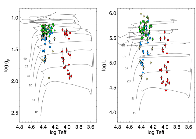
Figure 5: Hertzsprung-Russell diagram of the supergiant stars of this study compared with evolutionary tracks from Eckström et al. (2012). Left: spectroscopic HRD; Right: classic HRD. The different samples are shown in different colours: blue–MagE, green–FEROS, gold–VFTS.

Fig. 5, right-hand side, shows the Hertzsprung-Russell diagram (HRD) of the supergiants investigated by our spectroscopic study. We have used A${}_{\!\mbox{\scriptsize\,\sc v}}$ and bolometric correction BC as given in the tables and a distance modulus m-M = 18.494 mag (Pietrzynski et al., 2013) to obtain absolute bolometric magnitudes. The theoretical evolutionary tracks overplotted are from Eckström et al. (2012) and calculated for solar metallicity and with a rotation rate on the zero age main sequence of 40% of the critical break-up velocity. The evolved evolutionary status of our targets is obvious from the comparison with the tracks.

An alternative way to discuss stellar evolution, which has been introduced by Langer & Kudritzki (2014), is the use of the “spectroscopic” HRD (sHRD), which replaces the absolute bolometric magnitude by the logarithm of the flux-weighted gravity $\log\,g_{\!\mbox{\scriptsize\,\sc f}}$. The sHRD is particularly useful in cases where the stellar distances are uncertain. In addition, in situations where the distance is well know, the differential comparison of the position of supergiants relative to evolutionary tracks in the HRD versus the sHRD can reveal extreme outliers for which the stellar masses are not consistent with stellar evolution and the location in the HRD (see Langer & Kudritzki 2014). We, therefore, show the sHRD of our targets in the left-hand side panel of Fig. 5. While for some of our objects one might infer different masses from the inspection of the two diagrams, we do not see a reason to exclude objects from the sample.

4.2 Metallicity

The major focus of our work is the recalibration of the FGLR. Thus, we postpone the detailed investigation of the chemical composition of our sample to a forthcoming publication. However, since we have adopted a metallicity a factor of 0.4 lower than the Sun for our model atmosphere calculations and for the fit of the spectra, we need a straightforward check whether this assumption is basically correct. Therefore, we use two elements, Mg and Fe, as proxies for metallicity. Strong Mg lines are present in the spectra of both the BA and OB supergiants and, thus, we determined Mg abundances for the whole sample. The spectra of the BA show multiple Fe ii features, as well as weaker Fe i lines, that can be individually resolved at the resolution and SNR of our sample. On the other hand, the OB supergiants show only a handful of extremely weak Fe iii lines in their optical spectra, which makes the determination of iron abundances for these objects uncertain. We, thus, determine iron abundances only for the BA supergiant subsample.

4.2.1 Iron abundances from BA supergiants

Individual Fe abundances derived from our sample of BA supergiant stars are collected in Tab. 6. These are based on the set of spectral lines defined in Tab. 5. The mean and standard deviation of the BA sample is $\big{\langle}Fe/H\big{\rangle}\,=\,7.16\pm 0.11$ dex. There are no significant outliers; the median absolute deviation is 0.09 dex, indicating chemical homogeneity for the BA stars analysed in this work. In terms of relative values with respect to the Sun and the solar neighbourhood, our value corresponds to $\left[Fe/H\right]\,=\,-0.34,\,-0.36$ dex, depending on the reference value used for Fe: $7.50\pm 0.04$ dex for photospheric abundance of Fe in the Sun (Asplund et al., 2009) or $7.52\pm 0.04$ dex for the mean Fe abundance of a sample of B-type dwarf/giant stars in the solar neighbourhood (Nieva & Przybilla, 2012).

The derived Fe abundances from our BA sample agree well with the values obtained for classic Cepheids by Luck et al. (1998), $\left[Fe/H\right]\,=\,-0.35\pm 0.15$ dex, and more recently by Romaniello et al. (2008), $\left[Fe/H\right]\,=\,-0.33\pm 0.10$ dex. This is very encouraging, giving the different nature of the objects, analysis techniques and models that are employed in these studies, when compared to ours. This would give support to the idea that, for more distant galaxies, where metallicity studies of Cepheids are currently not possible, blue supergiant stars (in this particular case, BA-type supergiants) can be used as good proxies for the iron content of Cepheids, even though these objects belong to a somewhat older population.

4.2.2 Magnesium abundance throughout the sample

Individual Mg abundances derived for all the stars in the sample are presented in Tab. 6 (BA supergiants) and Tab. 7, 8 and  9 (OB supergiants). Before discussing the results, there are a few aspects to consider. First, Mg abundances are not affected by stellar evolution, hence we would expect for both samples to show a high degree of homogeneity. Secondly, the set of model atmosphere/line formation codes are different for the two groups (see previous sections). But, more importantly, whilst treated in non-LTE, the Mg model atom used is also not the same for both groups. Hence, slight differences in the zero point of both sub-samples are possible. But at the same time, each group should be highly homogeneous internally.

The mean and standard deviation of the BA subsample is $\big{\langle}Mg/H$⟩ = 7.33$\pm 0.07$ dex. For the OB subsample, we obtained $\big{\langle}Mg/H$⟩ = 7.20$\pm 0.12$ dex, a value which agrees well with the LMC B-supergiant studies by Dufton et al. (2006) and Trundle et al. (2007). As expected, both groups are individually highly homogeneous. Also, not totally unexpected given the different atomic data employed for each group, there is a zero point difference of 0.13 dex. Disregarding this difference, the value for the combined sample is $\big{\langle}Mg/H$⟩ = 7.24$\pm 0.14$ dex. There are arguments supporting the idea that the value from the BA sample should be preferred (for once, there are more lines included in the analysis; only Mg ii 4481 is observed in the OB supergiants). However, for the time being, we will adopt the mean value from the full sample as the representative value for the present-day Mg abundance in the LMC. Comparing our value with the Sun and solar neighbourhood (see references in previous section), we obtain $\left[Mg/H\right]\,=\,-0.36,\,-0.32$ dex (Sun: 7.60$\pm$0.04 dex; solar neighbourhood: 7.56$\pm$0.05).

Whilst a detailed discussion on the chemical abundances is deferred to a dedicated paper, we would like to mention here that our Mg abundance (an $\alpha$-element), regardless of the solar reference considered, agrees very well with the corresponding oxygen value obtained by Bresolin (2011) for a sample of LMC H ii regions, $12+\log\,(O/H)\,=\,8.36\pm\,0.10$ dex, or $\left[O/H\right]\,=\,-0.33\pm 0.10$ dex, reinforcing the concept that blue supergiants’ and H ii region abundances (based on the electronic temperature of the gas, the so-called direct method) yield consistent results at metallicities below solar.

Combining the Mg abundances with the previously discussed Fe abundances from the BA supergiants, it seems clear that our sample is chemically homogeneous, and that it shows a “metallicity” that corresponds to $\left[Z\right]\,=\,-0.35\pm 0.09$ dex, where Z represents the characteristic metallicity based on Fe (iron-group) and Mg ($\alpha$-element) abundances (weighted mean and sigma of their relative values with respect to the solar values). One can compare this result with the one obtained recently by Davies et al. (2015), based on the analysis of mid resolution IR spectra of a sample of 9 LMC red supergiant stars. Using LTE hydrostatic model atmospheres and detailed non-LTE calculations of Si i, Ti i and Fe i lines, these authors find $\left[Z\right]\,=\,-0.37\pm 0.14$ dex. We want to stress out once more that this agreement is remarkable, given the differences in the analysis techniques, model atmospheres, atomic data and nature of the objects analysed in this work.

4.3 Effects of spectral resolution

The Flux-weighted Gravity as defined by Kudritzki et al. (2003), $g_{\!\mbox{\scriptsize\,\sc f}}$$\equiv$ g/$T_{\!\mbox{\scriptsize\em eff}}^{4}$, requires the determination of surface gravity and effective temperature of the star. These fundamental parameters can in principle be easily determined from the quantitative analysis of the optical spectrum of B- and A-type supergiant stars, as shown in previous sections. But, whilst the surface gravity diagnostic lines (the hydrogen Balmer lines) are strong enough so that they remain accessible even at the low spectral resolutions required for the extragalactic work beyond the Local Group, this is not the case of the ionisation equilibria required for the determination of the effective temperature of BA-type supergiants, based on weak lines from neutral species (chiefly Mg i and Fe i). For OB supergiants, ionization equilibria (Si ii/iii/iv and He i/ii, see section 3.3) can still be used at low resolution, since the lines are strong enough and fairly isolated (Urbaneja et al., 2003).

To circumvent the issue of the lack of ionization equilibria for BA-supergiants at low spectral resolution Kudritzki et al. (2008) utilised the Balmer jump (Balmer discontinuity, located at $\sim$3650 Å) as an alternative diagnostic. This technique was then used in many of the extragalactic FGLR applications cited in the introduction. Our LMC observations of BA supergiants provide an excellent opportunity to compare the two alternative diagnostic methods. This comparison is carried out in the following subsections.

We also note that more recently Hosek et al. (2014) and Kudritzki et al. (2014) have introduced a technique, which determines $T_{\!\mbox{\tiny\em eff}}$ from information encoded in the spectra: the strength of He i lines and/or the relative strength of Ti ii and Fe ii lines. This alternative method has already been thoroughly tested by Hosek et al. (2014) and we, thus, refrain from an additional test here.

4.3.1 Consistency between Balmer jump and ionization equilibrium based temperatures

The relative flux calibration of the data collected during the two nights in October 2014 is regarded as very good, as is shown by the high consistency between the Balmer jump measurements for the different standard stars observed during these nights. It was not possible however to achieve the same satisfactory relative calibration for the data collected during the third night. Hence, the results shown in this section refer only to a subsample of our stars, 17 BA supergiant stars (see Tab. 10).

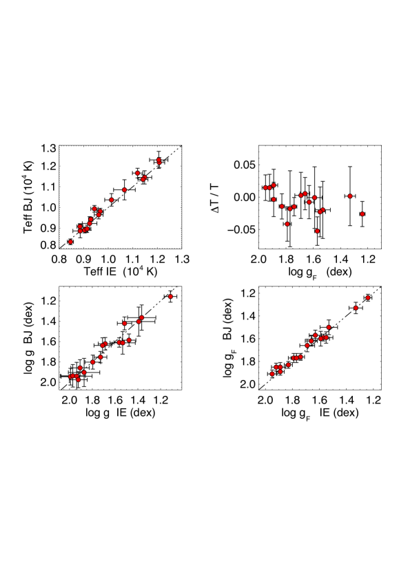
Figure 6: Comparison of Balmer jump based and IE based results. Clockwise: effective temperatures; relative difference in Teff against flux–weighted gravity; flux weighted gravities; surface gravities. See text for a discussion.

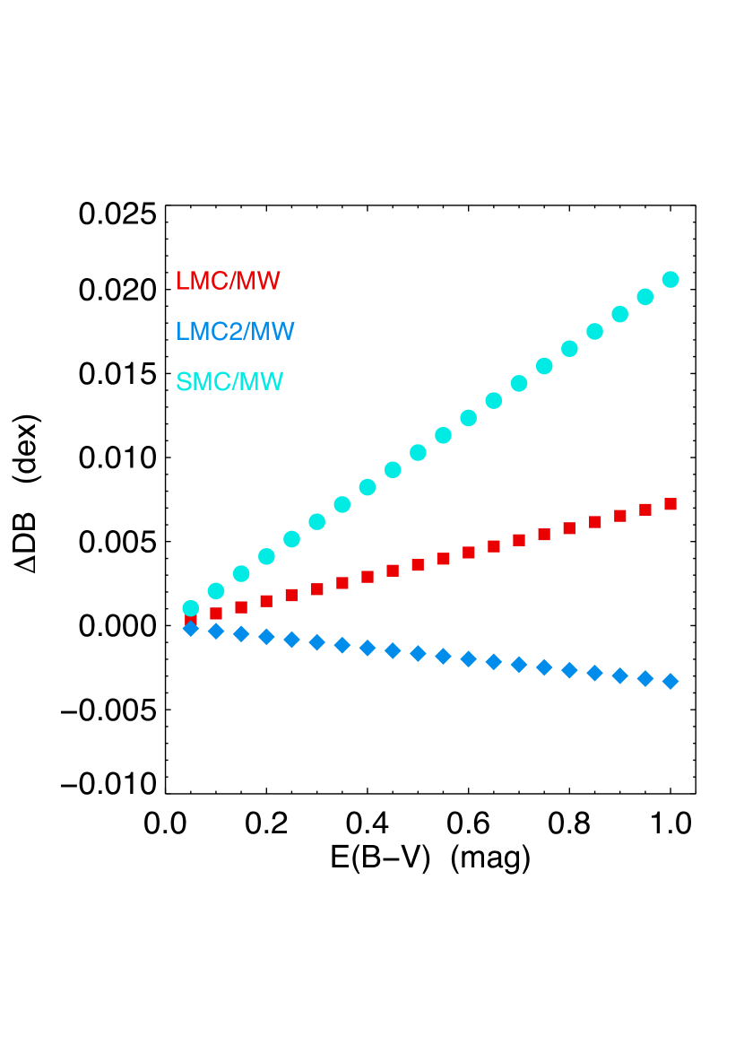
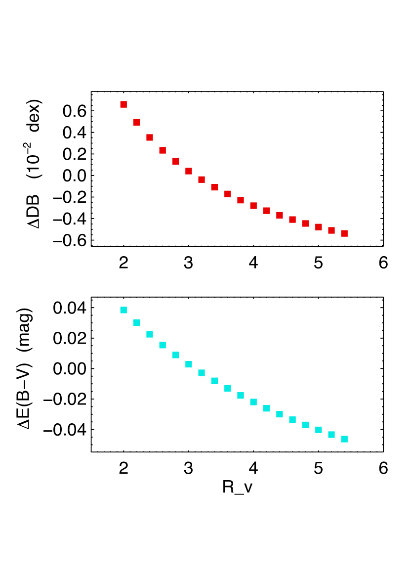
Figure 8: Effects of the reddening law on the Balmer jump. Different reddening laws are considered: MW–Cardelli et al. 1989, LMC and LMC2–Misselt et al. 1999, SMC–Gordon et al. 2003. See text for discussion.

First, we conducted two separated analyses, one considering the ionisation equilibrium of Mg i/ii and Fe i/ii, and a second one using the D${}_{\!\mbox{\scriptsize\,\sc b}}$ index as $T_{\!\mbox{\tiny\em eff}}$ indicator. The results are summarized in Fig. 6, and the measurements of the Balmer jump D${}_{\!\mbox{\scriptsize\,\sc b}}$ as defined in Kudritzki et al. (2008) are given in Tab 10. Within the uncertainties of the analyses, the results show a high consistency between the temperatures derived via the application of an ionisation equilibrium and the ones obtained through the D${}_{\!\mbox{\scriptsize\,\sc b}}$ index. As for the latter, the measurement of D${}_{\!\mbox{\scriptsize\,\sc b}}$ could be potentially affected by the particular form of the extinction law modifying the intrinsic spectral energy distribution of each star individually. However, as shown in Fig. 8, this is not the case. The left hand side of this figure illustrates the difference between the true D${}_{\!\mbox{\scriptsize\,\sc b}}$ index measured from a synthetic spectral energy distribution of a typical A0 supergiant star, reddened by the amount indicated in the x-axis, when considering different forms of the reddening law (MW–Cardelli et al. 1989, LMC–Misselt et al. 1999, SMC–Gordon et al. 2003), and the measured D${}_{\!\mbox{\scriptsize\,\sc b}}$ value under the assumption that the form of the extinction law is given by Cardelli et al. (1989), with $\mbox{R${}_{\!\mbox{\scriptsize\,\sc v}}$}/E\left(B-V\right)=3.1$. An error in D${}_{\!\mbox{\scriptsize\,\sc b}}$ of 0.02 dex, comparable to the accuracy achievable in external galaxies (i.e. Kudritzki et al., 2008; Urbaneja et al., 2008), would require the combination of a significantly different form of the extinction law (SMC versus MW) and a high reddening value, $E\left(B-V\right)\sim 0.9$ mag. It is very unlikely that a star showing such high reddening (hence extinction) would be selected for spectroscopic observations, since it will appear as a faint, reddish target.

The right-hand side of Fig. 8 illustrates the effects of assuming a fix R${}_{\!\mbox{\scriptsize\,\sc v}}$$\,=\,$3.1 value (for an extinction curve given by Cardelli et al. parametrisation) when our typical A0 star is reddened with different R${}_{\!\mbox{\scriptsize\,\sc v}}$ values (x-axis). It is also considered in this case that the observed photometric colour is V-I, hence there is a contribution from the translation from $E\left(V-I\right)$ to $E\left(B-V\right)$, which is R${}_{\!\mbox{\scriptsize\,\sc v}}$ dependent, also present. The lower right-hand side panel shows the difference in $E\left(B-V\right)$ (real minus recovered) for different values of R${}_{\!\mbox{\scriptsize\,\sc v}}$, whilst the upper panel displays the (negligible) effect on D${}_{\!\mbox{\scriptsize\,\sc b}}$ .

We conclude that the Balmer jump is in fact an excellent $T_{\!\mbox{\tiny\em eff}}$ discriminant in the B8–A3 spectral range, rivalling in accuracy with the standard techniques used at high spectral resolution. We note that this conclusions also agrees with the results obtained by Firnstein & Przybilla (2012), who studied a large sample of Milky Way BA supergiants. Fig. 6 also demonstrates that flux-weighted gravities are not systematically affected by the choice of the method used for the determination of $T_{\!\mbox{\tiny\em eff}}$.

4.3.2 Consistency between low and high spectral resolution results for the flux-weighted gravity.

In the preceding subsection we used our high spectral resolution observations to compare the results of the two alternative methods, the Balmer jump or ionization equilibria, as a constraint for the determination of effective temperature. However, in the extragalactic application of the FGLR-method for distance determinations spectra of moderate resolution of only 4.5 or 5 Å are used because of the faintess of the targets at large distances. The transition from high to moderate resolution could introduce systematic effects affecting temperatures and, most importantly, flux-weighted gravities.

In order to investigate these effects we degraded the resolution of the spectra of the BA supergiants in Tab. 10 to 5 Å and repeated the spectral analysis again using the Balmer jump for temperature (note that we adopted a general uncertainty of 0.02 dex for the Balmer jump to be consistent with the extragalactic work. This is larger than in the previous section and leads to larger $T_{\!\mbox{\tiny\em eff}}$ errors).

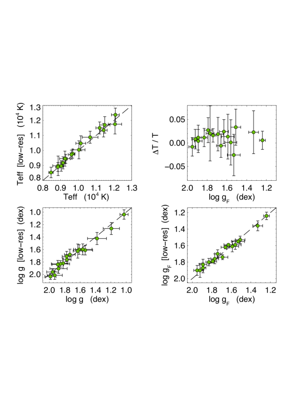
Figure 7: Comparison of flux-weighted gravities and temperatures derived from high- and low-resolution optical spectra. Clockwise: effective temperatures (based on IE at high-res, based on the Balmer jump at low-res); relative difference in Teff against flux–weighted gravity; flux weighted gravities; surface gravities. See text for a discussion.

Fig. 7 shows the comparison between temperatures and gravities obtained in this way with the values resulting from the ionization equilibrium analysis of the high resolution spectra. Within the error margins no systematic effects are found.

Table 10: BA Supergians results based on the Balmer jump as $T_{\!\mbox{\tiny\em eff}}$ indicator, at nominal and degraded spectral resolution.

Star	D${}_{\!\mbox{\scriptsize\,\sc b}}$	$T_{\!\mbox{\tiny\em eff}}$	$\log\,g_{\!\mbox{\scriptsize\,\sc f}}$	$T_{\!\mbox{\tiny\em eff}}$	$\log\,g_{\!\mbox{\scriptsize\,\sc f}}$
	(dex)	($\times 10^{4}$ K)	(dex)	($\times 10^{4}$ K)	(dex)
NGC 2004 8	0.21	1.1455$\pm$ 0.0290	1.66$\pm$ 0.06	1.1700$\pm$ 0.0248	1.74$\pm$ 0.03
Sk-65 67	0.29	0.9935$\pm$ 0.0075	1.59$\pm$ 0.03	1.0045$\pm$ 0.0192	1.59$\pm$ 0.05
Sk-67 19	0.43	0.8865$\pm$ 0.0150	1.60$\pm$ 0.07	0.8980$\pm$ 0.0167	1.61$\pm$ 0.06
Sk-67 137	0.16	1.2300$\pm$ 0.0375	1.50$\pm$ 0.07	1.1750$\pm$ 0.0215	1.55$\pm$ 0.02
Sk-67 140	0.36	0.9815$\pm$ 0.0070	1.83$\pm$ 0.03	0.9790$\pm$ 0.0138	1.80$\pm$ 0.05
Sk-67 141	0.49	0.8910$\pm$ 0.0065	1.91$\pm$ 0.04	0.8965$\pm$ 0.0108	1.90$\pm$ 0.06
Sk-67 143	0.29	1.0365$\pm$ 0.0140	1.59$\pm$ 0.05	1.0475$\pm$ 0.0189	1.53$\pm$ 0.05
Sk-67 155	0.38	0.9430$\pm$ 0.0045	1.76$\pm$ 0.03	0.9440$\pm$ 0.0144	1.70$\pm$ 0.05
Sk-67 157	0.19	1.1355$\pm$ 0.0200	1.62$\pm$ 0.05	1.1350$\pm$ 0.0301	1.62$\pm$ 0.02
Sk-67 170	0.39	0.9648$\pm$ 0.0090	1.89$\pm$ 0.03	0.9725$\pm$ 0.0143	1.87$\pm$ 0.06
Sk-67 171	0.17	1.2175$\pm$ 0.0220	1.57$\pm$ 0.05	1.2375$\pm$ 0.0245	1.59$\pm$ 0.01
Sk-69 2A	0.62	0.8340$\pm$ 0.0065	1.85$\pm$ 0.04	0.8535$\pm$ 0.0140	1.90$\pm$ 0.09
Sk-69 24	0.26	1.0855$\pm$ 0.0220	1.77$\pm$ 0.04	1.0880$\pm$ 0.0103	1.76$\pm$ 0.06
Sk-69 39A	0.47	0.8970$\pm$ 0.0080	1.85$\pm$ 0.04	0.9175$\pm$ 0.0109	1.83$\pm$ 0.06
Sk-69 113	0.25	0.9230$\pm$ 0.0150	1.33$\pm$ 0.05	0.9455$\pm$ 0.0196	1.36$\pm$ 0.06
Sk-69 299	0.26	0.9080$\pm$ 0.0065	1.24$\pm$ 0.03	0.8900$\pm$ 0.0158	1.24$\pm$ 0.05
Sk-70 45	0.23	1.1660$\pm$ 0.0210	1.77$\pm$ 0.04	1.1500$\pm$ 0.0185	1.79$\pm$ 0.02

Note. — First (second) $T_{\!\mbox{\tiny\em eff}}$–$\log\,g_{F}$ pair corresponds to the values derived at nominal (degraded) spectral resolution. The uncertainty in the measured D${}_{\!\mbox{\scriptsize\,\sc b}}$ index at the nominal resolution is in all cases smaller than 0.01 dex. See text for details.

4.4 Individual reddenings and total to selective extinction ratios, E(B-V) and R${}_{\!\mbox{\scriptsize\,\sc v}}$.

Once the fundamental parameters of each star are known, we calculate a tailored model for each object. By comparing the predicted spectral energy distribution with the observed one, individual filter pass-band integrated reddening values E(B-V) and R${}_{\!\mbox{\scriptsize\,\sc v}}$= A_V/E(B-V) can be derived for each object. Our procedure to determine the reddening, E(B-V) and R${}_{\!\mbox{\scriptsize\,\sc v}}$, is based entirely on the use of observed photometric colours and magnitudes, which are then compared to colours obtained from the spectral energy distribution of our model atmospheres. We do not use monochromatic fluxes for the determination of E(B-V) and R${}_{\!\mbox{\scriptsize\,\sc v}}$.

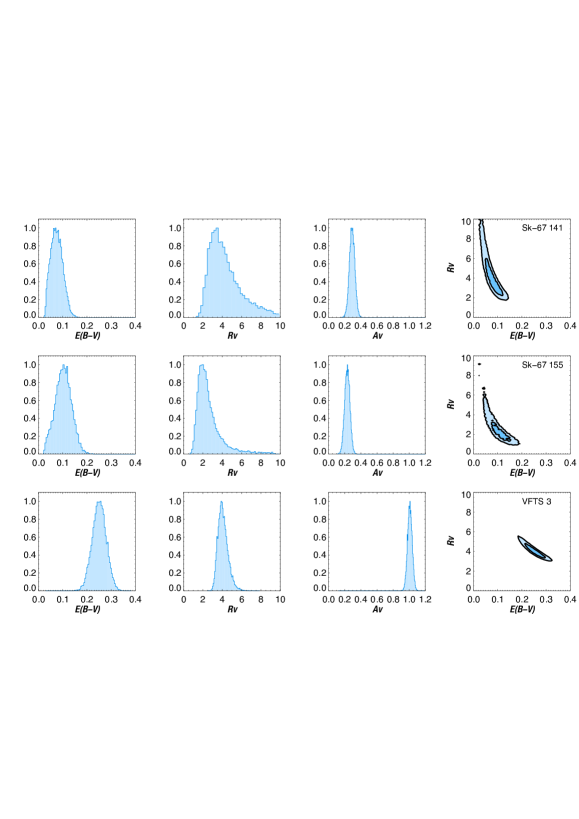
Figure 9: Monte Carlo Marko Chain determination of E(B-V),R${}_{\!\mbox{\scriptsize\,\sc v}}$ and A${}_{\!\mbox{\scriptsize\,\sc v}}$ for the stars Sk-67 141, Sk-67 155 and VFTS 3. For each target posterior probability distribution functions for each variable are displayed together with the conditional E(B-V)–R${}_{\!\mbox{\scriptsize\,\sc v}}$ probability function, showing the isocontours enclosing 67%and 95% of the solutions.

We proceed as follows: (1) a pair of monochromatic E(4405-5495) and R${}_{5495}\,=\,$A₅₄₉₅/E(4405-5495) values are drawn. This is done because the reddening laws, for which we have applied our procedure (see below), are defined as monochromatic laws and the key parameter characterizing them is R₅₄₉₅. (2) the synthetic spectral energy distribution, SED, predicted by the tailored model calculated with the results obtained in our spectroscopic analysis, is then reddened using the Cardelli et al. (1989) monochromatic reddening law (the use of other reddening laws has no significant effect on the final FGLR, see below); (3) the corresponding B-V, V-J, V-H and V-Ks model colours are calculated from the reddened SED; (4) the differences between model and observed colours are calculated and enter the calculation of the cost function. Errors of the colour differences account for the observed values and a contribution from the synthetic photometry (assumed to be a constant 0.01 mag); (5) steps 1 to 4 are repeated in a Monte Carlo Markov Chain (MCMC) procedure, minimizing the cost function (a $\chi^{2}$ with 2 degrees of freedom, since we are using four colours two solve simultaneously for two variables). Fig. 9 displays the results of our MCMC procedure for three of the targets in our sample. Posterior probability distribution functions for E(B-V),R${}_{\!\mbox{\scriptsize\,\sc v}}$ and A${}_{\!\mbox{\scriptsize\,\sc v}}$ are shown, as well as the conditional E(B-V)–R${}_{\!\mbox{\scriptsize\,\sc v}}$ distribution function, with the isocontours enclosing 67% and 95% of the solutions obtained. We determine mean values and (asymmetric) uncertainties from the posterior probability distribution functions. Note that R₅₄₉₅ and E(4405-5495) are converted to the corresponding filter integrated quantities using the final model atmospheres SEDs. These values of R${}_{\!\mbox{\scriptsize\,\sc v}}$ and E(B-V) are then used to calculate the extinction A${}_{\!\mbox{\scriptsize\,\sc v}}$. Fig. 10 summarizes the results for the full sample. Whilst the uncertainties of R${}_{\!\mbox{\scriptsize\,\sc v}}$ become large for small values of reddenig, the extinction A${}_{\!\mbox{\scriptsize\,\sc v}}$ remains well constrained with relatively small errors. The reason is explained by the isocontours shown in Fig. 9, which demonstrate that errors in R${}_{\!\mbox{\scriptsize\,\sc v}}$ and E(B-V) are anticorrelated.

Note that whilst IRAC/Spitzer photometry is available for most of the sample, we used it just as a posterior validation of the result, and not in the derivation of R${}_{\!\mbox{\scriptsize\,\sc v}}$.

We decided to work with line-of-sight values, i.e. we do not consider separated contributions for the Milky Way and the LMC. The values derived for the full sample are collected in Tab. 6 through Tab. 9. There are 4 stars in common with the work by Gordon et al. (2003): Sk-69 270, Sk-67 2, Sk-68 26 and VFTS 696 (aka Sk-68 140). Note that Gordon et al. (2003) implicitly “corrected” for Galactic extinction, since they use lightly reddened LMC stars as comparisons to estimate these values (whilst we use model atmospheres instead). Nonetheless, our E(B-V) and R${}_{\!\mbox{\scriptsize\,\sc v}}$ values are in agreement with theirs, when considering our larger uncertainties for R${}_{\!\mbox{\scriptsize\,\sc v}}$; our derived E(B-V) values are $\sim$0.05–0.08 mag higher, which can be easily understood as the combined Galactic and LMC contributions to reddening of the stars used as reference by these authors (Gordon et al., 2003, see Tab. 2). Unfortunately a comparison with the recent study by Maíz Apellániz et al. (2014) is not possible since we do not have stars in common with this work.

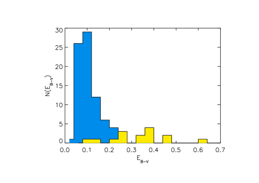
Figure 11: Histogram of observed E(B-V) values. The yellow histograms correspond to the subsample of stars in the Tarantula region (VFTS sample).

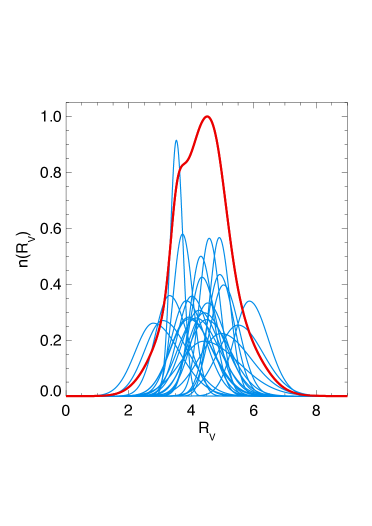
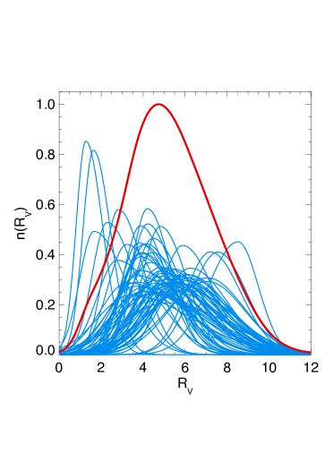
Figure 12: Probability distribution N(R${}_{\!\mbox{\scriptsize\,\sc v}}$) for all targets with E(B-V)$\geq$0.15 mag (left,red), and E(B-V)$<$0.15 mag. The distributions are obtained by adding the assymetric Gaussian distributions of all individual targets (plotted in blue) and subsequent re-normalization.

The E(B-V) distribution is shown in Fig. 11. For the sample of targets observed with MagE and FEROS the distribution peaks strongly at E(B-V) = 0.08 mag. However, there are also line-of-sights with significantly higher reddening, in particular, for targets located in the Tarantula Nebula shown as a yellow histogram in the plot. Of particular, interest is the distribution of R${}_{\!\mbox{\scriptsize\,\sc v}}$-values. However, because of the relatively large errors of R${}_{\!\mbox{\scriptsize\,\sc v}}$ a simple histogram is not useful. Instead, we construct a probability distribution for the total sample by assuming asymmetric Gaussian distributions for each individual star, which are them summed up to obtain the total distribution. The results are shown in Fig. 12 for target subsamples with E(B-V) larger and smaller than 0.15 mag respectively. It is evident that we encounter a relatively wide range of R${}_{\!\mbox{\scriptsize\,\sc v}}$ values between 3 and 6,in agreement with previous work (see for example Maíz Apellániz et al., 2017). Also worth mentioning are the three cases with very low values of R${}_{\!\mbox{\scriptsize\,\sc v}}$ (namely Sk -67 137, Sk -67 154 and Sk -67 170). Interestingly, all these three objects are members of the cluster NGC 2004, but they are not spatially concentrated (see Fig. 16 in Evans et al. 2006). These putatively low values are not modified when using any other available photometry. In this regard, we would like to point out that there are indications of low values of R${}_{\!\mbox{\scriptsize\,\sc v}}$ in lines of sight of SN Ia, ranging from R${}_{\!\mbox{\scriptsize\,\sc v}}$= 1.0 to R${}_{\!\mbox{\scriptsize\,\sc v}}$= 2.5 (Cikota et al., 2016).

Finally, we note that the standard assumption for extragalactic distance determinations using stellar distance indicators such as cepheids or blue supergiants is to use a standard value of R${}_{\!\mbox{\scriptsize\,\sc v}}$ = 3.1 or 3.3. However, Fig. 11 indicates that this may introduce systematic errors, in particular, with respect to the ambitious goal to increase the precision of the Hubble constant to a few percent (see, for instance Riess et al., 2011).

5 Flux-weighted Gravity–Luminosity Relationship of LMC supergiants

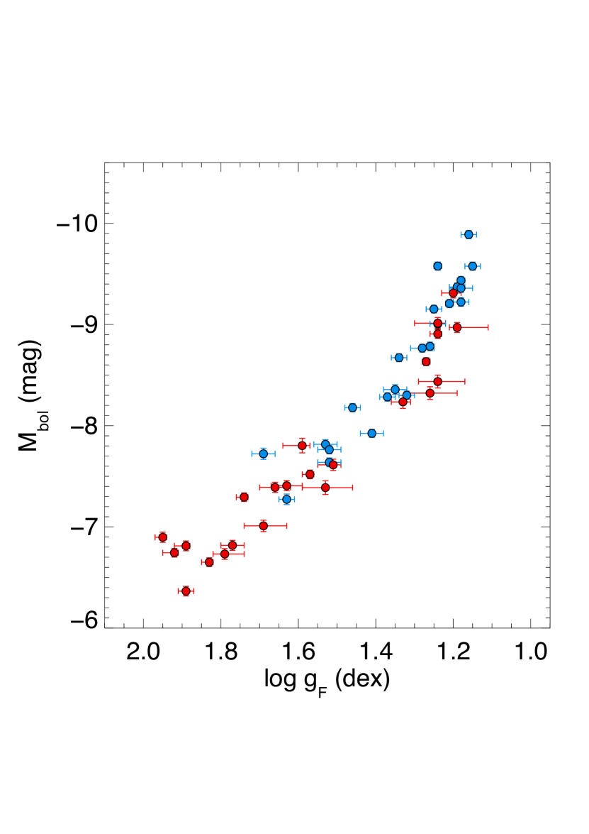
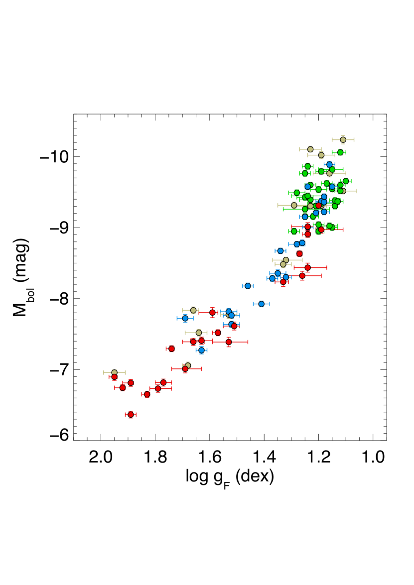
Figure 13: Observed FGLR of LMC supergiants. Left: Sample of supergiants observed with MagE (BA-supergiants: red, OB-supergiants: blue). Right: The full sample including targets observed with FEROS (green) and VFTS (gold).

Fig. 13 shows a plot of absolute bolometric magnitudes versus flux-weighted gravities. As mentioned before, we used a distance modulus to the LMC of m-M = 18.494 mag (Pietrzynski et al., 2013) together with the values of E(B-V), R${}_{\!\mbox{\scriptsize\,\sc v}}$ and bolometric correction as given in the tables to obtain M_bol. The left hand side shows the the subsample of supergiants observed with the MagE spectrograph only. This was the starting point of our investigation to accomplish a new calibration of the FGLR. Realizing that the data indicate a change in the slope of the FGLR for $\log\,g_{\!\mbox{\scriptsize\,\sc f}}$ values smaller than 1.30 dex we decided to supplement our MagE sample with the FEROS and VLT/FLAMES spectra to enlarge the sample. The full sample is then given on the right hand side and the change in the slope is now very apparent.

A straightforward fit to the data is to introduce a flux-weighted gravity $\log\,g_{\!\mbox{\scriptsize\,\sc f}}^{\!\mbox{\scriptsize\,break}}$, where the slope of the FGLR changes. For flux-weighted gravities larger than or equal to this value we adopt a FGLR of the form of eq. (1) and determine the coefficients $a$ and $b$ by a linear regression that accounts for errors both in $\log\,g_{\!\mbox{\scriptsize\,\sc f}}$ and M_bol. For flux-weighted gravities smaller than $\log\,g_{\!\mbox{\scriptsize\,\sc f}}^{\!\mbox{\scriptsize\,break}}$ we than adopt an FGLR with a different slope, which meets the high gravity FGLR at $\log\,g_{\!\mbox{\scriptsize\,\sc f}}^{\!\mbox{\scriptsize\,break}}$. This latter slope is obtained by $\chi^{2}$-minimalization again accounting for errors both in $\log\,g_{\!\mbox{\scriptsize\,\sc f}}$ and M_bol. In this way we have

$$\mbox{$\log\,g_{\!\mbox{\scriptsize\,\sc f}}$}\,\geq\,\log\,g_{\!\mbox{\scriptsize\,\sc f}}^{\!\mbox{\scriptsize\,break}}:\,M_{\rm bol}\,=\,a(\mbox{$\log\,g_{\!\mbox{\scriptsize\,\sc f}}$}\,-\,1.5)\,+\,b$$ (2)

and

$$\mbox{$\log\,g_{\!\mbox{\scriptsize\,\sc f}}$}\leq\,\log\,g_{\!\mbox{\scriptsize\,\sc f}}^{\!\mbox{\scriptsize\,break}}\,:\,M_{\rm bol}\,=\,a_{\rm low}(\mbox{$\log\,g_{\!\mbox{\scriptsize\,\sc f}}$}\,-\,\log\,g_{\!\mbox{\scriptsize\,\sc f}}^{\!\mbox{\scriptsize\,break}})\,+\,b_{\!\mbox{\scriptsize\,break}}$$ (3)

with

$$b_{\!\mbox{\scriptsize\,break}}\,=\,a(\log\,g_{\!\mbox{\scriptsize\,\sc f}}^{\!\mbox{\scriptsize\,break}}\,-\,1.5)\,+\,b.$$ (4)

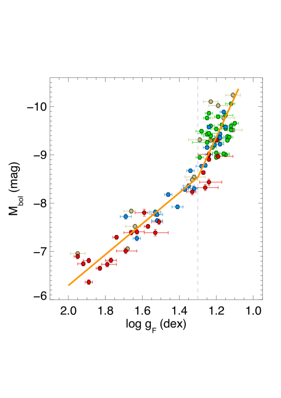
Figure 14: Linear regression fits (orange) to the observed FGLR of Fig. 13 for the flux-weighted gravity intervals log g_F larger or smaller than 1.29 dex (see text). The grey vertical dashed line indicates the the flux-weighted gravity log g${}_{F}^{break}$ = 1.29 dex, where the slopes of the regressions change.

We select $\log\,g_{\!\mbox{\scriptsize\,\sc f}}^{\!\mbox{\scriptsize\,break}}=1.30$ dex and obtain a = 3.20$\pm$0.08, b = -7.90$\pm$0.02 mag and a_low = 8.34$\pm$0.25. The standard deviations from the fit are $\sigma\,=\,0.24$ mag for $\log\,g_{\!\mbox{\scriptsize\,\sc f}}\geq 1.30$ dex and 0.42 mag for $\log\,g_{\!\mbox{\scriptsize\,\sc f}}<1.30$ dex. Fig. 14 shows the corresponding fit to the data. We note that for gravities above $\log\,g_{\!\mbox{\scriptsize\,\sc f}}^{\!\mbox{\scriptsize\,break}}$ the slope obtained for our LMC sample is slightly lower than the slope found in the original calibration by Kudritzki et al. (2008), while the intercept corresponds to absolute magnitudes 0.12 mag fainter ($a_{\rm old}$ = 3.41$\pm$0.16, $b_{\rm old}$ = -8.02$\pm$0.04 mag).

The detection of an obvious break in the slope of the FGLR is a surprise. The previous data sets leading to the detection of the FGLR (Kudritzki et al., 2003) and used for the first calibration (Kudritzki et al., 2008) contained only a few objects with flux-weighted gravities lower than $\log\,g_{\!\mbox{\scriptsize\,\sc f}}^{\!\mbox{\scriptsize\,break}}$ and did not provide any hints that an FGLR with two slopes would be needed to fit the data. On the other hand, as discussed in these early papers, the theory of stellar evolution predicts a mildly curved FGLR with a steeper slope at the high luminosity end, in particular at lower metallicity. Observationally, a first indication in this regard was recognized by Hosek et al. (2014) in the FGLR observations of NGC 3109 and a combined sample of blue supergiants of all FGLR-studied galaxies so far.

As first noticed by Kudritzki et al. (2008), in the simple interpretation of the FGLR as a result of stellar evolution across the HRD with constant luminosity and mass the slope of the FGLR a is related to the exponent $x$ of the mass-luminosity relationship

$$L\sim M^{x}$$ (5)

through the simple equation

$$a=-2.5{x\over 1-x}.$$ (6)

A small exponent $x$ as predicted by stellar evolution theory for very massive stars would result in a steep slope of the FGLR (for instance $x$ = 1.5 would lead to $a$ = 7.5), whereas a larger exponent x as encountered for stars of lower mass would flatten the slope of the FGLR ($x$ = 4 would result in $a$ = 3.3).

However, in reality the situation is more complicated. Massive stars after having left the main sequence phase do not exactly evolve at constant luminosity and their masses, when they enter the blue supergiant stage, depend on the history of mass-loss. Meynet et al. (2015) have studied these effects in detail using state-of-the-art stellar evolution calculations and confirmed the general concept of the FGLR. While this work investigated the role of metallicity and the question whether blue supergiants are mostly in an evolutionary phase evolving towards or back from the red supergiant stage, it did not focus on the slope of the FGLR at its high luminosity end. However, a careful inspection of their population synthesis results based on stellar evolution, in particular their Figure 9 (right hand side), indicates that the FGLR should indeed significantly steepen for flux-weighted gravities lower than 1.30 dex. A detailed extension of this work for the metallicity of the LMC (their Figure 9 is for solar metallicity) concentrating on the high luminosity end of the FGLR and also re-investigating the role of mass-loss on the main sequence and during the blue supergiant stage would be a crucial step to understand whether stellar evolution theory reproduces the observed FGLR of our LMC sample of blue supergiants.

6 Conclusions and future work

The results obtained in this study of LMC blue supergiant stars confirm the existence of a tight relationship between absolute bolometric magnitude and flux-weighted gravity. However, from the much larger sample investigated relative to previous calibration attempts it is now evident that the FGLR changes its slope at a flux weighted gravity of $\log\,g_{\!\mbox{\scriptsize\,\sc f}}$$\,\approx 1.29$ dex. For lower gravities the relationship becomes significantly steeper and shows a somewhat larger scatter. As noted in the previous section, it is not clear at this point whether stellar evolution theory is able to reproduce and explain the observations presented here. An investigation of this question will require a detailed study combining population synthesis and stellar evolution in future work.

The regression fit applied to the observed FGLR data of our LMC sample provides an accurate new calibration of the relationship, which can be used for distance determinations. An obvious next step for future work will be the application of this new calibration for improved distance determinations to the set of galaxies for which blue supergiant observations have already been carried out or will be obtained in the near future. This application will include a careful investigation how the uncertainty of the slope at the upper end affects the accuracy of the distances determined. Since the FGLR data in the galaxies studied so far usually cover a wide range in luminosity and flux-weighted gravity, we are optimistic that the new calibration will yield accurate distances. The important advantage of the FGLR-method for distance determinations is that reddening and extinction, including variations of the reddening law, can be determined individually for each stellar target by the combination of spectroscopy and photometry as demonstrated in this work. This is of particular importance in all situations, where R${}_{\!\mbox{\scriptsize\,\sc v}}$, the ratio of visual extinction to reddening, varies over a wide range in a similar way as we have found for the LMC in this work. We note that extragalactic distance determinations using Cepheid stars usually assume a standard reddening law with R${}_{\!\mbox{\scriptsize\,\sc v}}$= 3.1 to either calculate “reddening-free” magnitudes or to apply a reddening correction to apparent distance moduli obtained in different filter passbands. Even in cases where the HST photometry of Cepheids is extended to the H-band in the near-infrared, this has the potential to introduce systematic errors of a few percent, when the reddening is a few tenths of a magnitude and the deviations from the standard reddening law are substantial. In this sense it will be interesting to compare distances obtained with the FGLR with distances using Cepheids and also with other methods such as the tip of the red giant branch. In view of the ambitious goal to determine the Hubble constant with a precision of one percent (Riess et al., 2011) the FGLR-method with the new calibration obtained in this work can contribute to investigate the role of systematic effects for the determination of extragalactic distances.

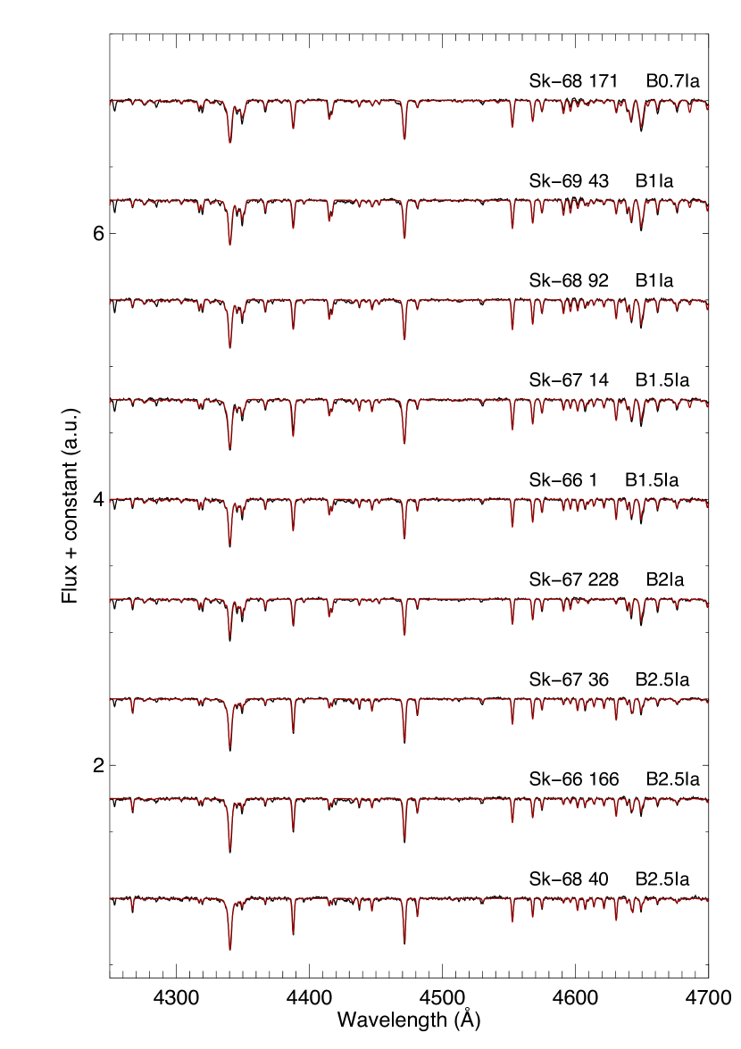
Figure 2: Example fits for some OB supergiants of our sample as a function of spectral type.

Figure 10: E(B-V), R${}_{\!\mbox{\scriptsize\,\sc v}}$, A${}_{\!\mbox{\scriptsize\,\sc v}}$ and uncertainties for the full sample. (a) R${}_{\!\mbox{\scriptsize\,\sc v}}$ vs. E(B-V). (b) Possitive (blue) and negative (red) uncertatinties in R${}_{\!\mbox{\scriptsize\,\sc v}}$ vs. E(B-V). (c) Possitive (blue) and negative (red) uncertainties in A${}_{\!\mbox{\scriptsize\,\sc v}}$ vs. E(B-V).

Appendix A Photometric data used in this investigation

Table 11: LMC Supergiants – Optical photometry.

Star	V	B-V	U-B	Reference
N11 24	13.45	-0.05	-0.87	Brunet et al. (1975)
N11 36	13.72	-0.15	$\cdots$	Evans et al. (2006)
N11 54	14.10	-0.06	$\cdots$	Evans et al. (2006)
NGC 2004 8	12.43	-0.03	$\cdots$	Evans et al. (2007)
NGC 2004 12	13.39	-0.20	$\cdots$	Evans et al. (2006)
NGC 2004 21	13.67	-0.14	$\cdots$	Evans et al. (2006)
NGC 2004 22	13.77	-0.17	$\cdots$	Evans et al. (2006)
Sk-65 67	11.44	0.05	-0.31	Ardeberg et al. (1972)
Sk-66 1	11.61	-0.06	-0.86	Isserstedt (1982)
Sk-66 5	10.73	-0.03	-0.78	Ardeberg et al. (1972)
Sk-66 15	12.81	-0.12	-0.95	Isserstedt (1979)
Sk-66 23	13.09	0.08	-0.64	Isserstedt (1979)
Sk-66 26	12.91	-0.05	-0.81	Isserstedt (1975)
Sk-66 27	11.82	0.02	-0.74	Isserstedt (1975)
Sk-66 35	11.60	-0.07	-0.89	Nicolet (1978)
Sk-66 36	11.35	0.07	-0.76	Isserstedt (1975)
Sk-66 37	12.98	-0.09	-0.89	Isserstedt (1979)
Sk-66 50	10.63	0.02	-0.67	Ardeberg et al. (1972)
Sk-66 106	11.72	-0.08	-0.91	Isserstedt (1975)
Sk-66 118	11.81	-0.05	-0.86	Nicolet (1978)
Sk-66 166	11.71	-0.04	-0.79	Ardeberg et al. (1972)
Sk-67 2	11.26	0.08	-0.77	Ardeberg et al. (1972)
Sk-67 14	11.52	-0.10	-0.91	Ardeberg et al. (1972)
Sk-67 19	11.19	0.14	-0.10	Ardeberg et al. (1972)
Sk-67 28	12.28	-0.14	-0.97	Isserstedt (1982)
Sk-67 36	12.01	-0.08	-0.81	Isserstedt (1975)
Sk-67 78	11.26	-0.04	-0.73	Ardeberg et al. (1972)
Sk-67 90	11.29	-0.09	-0.90	Ardeberg et al. (1972)
Sk-67 112	11.90	-0.13	-0.98	Ardeberg et al. (1972)
Sk-67 133	12.59	-0.05	-0.75	Isserstedt (1975)
Sk-67 137	11.93	0.04	-0.58	Ardeberg et al. (1972)
Sk-67 140	12.42	0.07	-0.23	Ardeberg et al. (1972)
Sk-67 141	12.01	0.07	-0.03	Ardeberg et al. (1972)
Sk-67 143	11.46	0.05	-0.42	Ardeberg et al. (1972)
Sk-67 150	12.24	-0.11	-0.92	Isserstedt (1975)
Sk-67 154	12.61	-0.06	-0.87	Isserstedt (1979)
Sk-67 155	11.60	0.09	-0.18	Ardeberg et al. (1972)
Sk-67 157	11.95	0.00	-0.51	Ardeberg et al. (1972)
Sk-67 169	12.18	-0.12	-0.90	Isserstedt (1975)
Sk-67 170	12.48	0.05	-0.22	Ardeberg et al. (1972)
Sk-67 171	12.04	-0.03	-0.57	Ardeberg et al. (1972)
Sk-67 172	11.88	-0.07	-0.81	Ardeberg et al. (1972)
Sk-67 173	12.04	-0.12	-0.96	Isserstedt (1975)
Sk-67 201	9.87	0.07	$\cdots$	Feast et al. (1960)
Sk-67 204	10.87	0.04	-0.53	Ardeberg et al. (1972)
Sk-67 206	12.00	-0.11	-0.95	Isserstedt (1975)
Sk-67 228	11.49	-0.05	-0.82	Ardeberg et al. (1972)
Sk-67 256	11.90	-0.08	-0.89	Isserstedt (1975)
Sk-68 26	11.63	0.12	-0.78	Gordon et al. (2003)
Sk-68 40	11.71	-0.07	-0.79	Ardeberg et al. (1972)
Sk-68 41	12.01	-0.14	-0.97	Isserstedt (1982)
Sk-68 45	12.03	-0.11	-0.94	Ardeberg et al. (1972)
Sk-68 92	11.71	-0.07	-0.88	Ardeberg et al. (1972)
Sk-68 111	12.01	-0.08	-0.89	Ardeberg et al. (1972)
Sk-68 171	12.01	-0.09	-0.89	Ardeberg et al. (1972)
Sk-69 2A	12.47	0.23	0.20	Ardeberg et al. (1972)
Sk-69 24	12.52	0.10	-0.41	Ardeberg et al. (1972)
Sk-69 39A	12.35	0.10	-0.17	Isserstedt (1975)
Sk-69 43	11.94	-0.07	-0.88	Ardeberg et al. (1972)
Sk-69 82	10.92	0.04	-0.57	Ardeberg et al. (1972)
Sk-69 89	11.39	-0.05	-0.82	Isserstedt (1975)
Sk-69 113	10.71	0.09	-0.42	Isserstedt (1979)
Sk-69 170	10.34	0.13	-0.52	Ardeberg et al. (1972)
Sk-69 214	12.19	0.01	-0.84	Isserstedt (1975)
Sk-69 228	12.12	0.07	-0.76	Isserstedt (1975)
Sk-69 237	12.08	-0.03	-0.86	Isserstedt (1975)
Sk-69 270	11.27	0.14	-0.66	Ardeberg et al. (1972)
Sk-69 274	11.21	0.04	-0.74	Ardeberg et al. (1972)
Sk-69 299	10.24	0.23	-0.26	Ardeberg et al. (1972)
Sk-70 45	12.53	0.01	-0.46	Isserstedt (1975)
Sk-70 78	11.29	-0.08	-0.89	Ardeberg et al. (1972)
Sk-70 111	11.85	-0.07	-0.87	Ardeberg et al. (1972)
Sk-70 120	11.59	-0.06	-0.88	Ardeberg et al. (1972)
Sk-71 14	10.62	0.09	-0.45	Ardeberg et al. (1972)
Sk-71 42	11.17	-0.04	-0.88	Isserstedt (1982)
VFTS 3	11.59	0.11	-0.73	Feitzinger & Isserstedt (1983)
VFTS 28	13.40	0.31	-0.71	Brunet et al. (1975)
VFTS 69	13.59	0.17	$\cdots$	Evans et al. (2011)
VFTS 82	13.61	-0.06	$\cdots$	Evans et al. (2011)
VFTS 232	14.52	0.50	$\cdots$	Evans et al. (2011)
VFTS 270	14.35	-0.07	$\cdots$	Evans et al. (2011)
VFTS 302	15.53	0.32	$\cdots$	Evans et al. (2011)
VFTS 315	14.81	0.03	$\cdots$	Evans et al. (2011)
VFTS 431	12.05	0.11	$\cdots$	Selman et al. (1999)
VFTS 533	11.82	0.29	$\cdots$	Selman et al. (1999)
VFTS 590	12.49	0.22	$\cdots$	Selman et al. (1999)
VFTS 696	12.74	0.09	-0.79	Isserstedt (1975)
VFTS 732	13.00	0.20	-0.66	Isserstedt (1982)
VFTS 831	13.04	0.29	$\cdots$	Evans et al. (2011)
VFTS 867	14.63	0.13	$\cdots$	Evans et al. (2011)

Note. — Unfortunately, individual errors in the photometric measurements for the full sample are not readily available. Many of the works do not provide this valuable information. In what follows, we list the uncertainties quoted in the those references listed: a) Ardeberg et al. (1972) : sig(V)=0.017, sig(B-V)=0.013, sig(U-B)=0.017 b) Isserstedt (1975, 1979, 1982) : sig(V)=0.025, sig(B-V)=0.020, sig(U-B)=0.025 c) Nicolet (1978) : sig(V)=0.02, sig(B-V)=0.015, sig(U-B)=0.02 d) Gordon et al. (2003) – for Sk-68 26: sig(V)=0.003, sig(B-V)=0.002, sig(U-B)=0.001. In lieu of this information being missing for all the other references, we adopted a flat error of sig(B-V)=0.02 mag and sig(V) = 0.02 mag for all the optical photometry used in this work.

Table 12: LMC Supergiants – 2MASS photometry (Skrutskie et al., 2006).

Star	SSTISAGEMC	J	H	Ks
		(mag)	(mag)	(mag)
N11 24	J045532.92-662527.7	13.529 $\pm$ 0.022	13.602 $\pm$ 0.025	13.633 $\pm$ 0.030
N11 36	J045740.99-662956.6	13.937 $\pm$ 0.029	13.956 $\pm$ 0.037	14.007 $\pm$ 0.032
N11 54	J045718.33-662559.7	14.080 $\pm$ 0.023	14.080 $\pm$ 0.025	14.110 $\pm$ 0.032
NGC 2004 8	J053040.09-671638.0	12.296 $\pm$ 0.022	12.278 $\pm$ 0.027	12.263 $\pm$ 0.026
NGC 2004 12	J053037.48-671653.6	13.847 $\pm$ 0.026	13.928 $\pm$ 0.029	13.923 $\pm$ 0.035
NGC 2004 21	J053042.02-672141.7	14.087 $\pm$ 0.035	14.153 $\pm$ 0.041	14.166 $\pm$ 0.048
NGC 2004 22	J053047.33-671723.3	13.889 $\pm$ 0.036	13.849 $\pm$ 0.050	13.820 $\pm$ 0.063
Sk-65 67	J053435.20-653852.8	11.168 $\pm$ 0.022	11.189 $\pm$ 0.024	11.105 $\pm$ 0.023
Sk-66 1	J045219.10-664353.2	11.656 $\pm$ 0.023	11.627 $\pm$ 0.023	11.665 $\pm$ 0.028
Sk-66 5	J045330.03-665528.1	10.797 $\pm$ 0.021	10.808 $\pm$ 0.024	10.810 $\pm$ 0.023
Sk-66 15	J045522.35-662819.0	13.020 $\pm$ 0.022	13.089 $\pm$ 0.024	13.090 $\pm$ 0.026
Sk-66 23	J045617.53-661818.9	12.839 $\pm$ 0.024	12.805 $\pm$ 0.026	12.761 $\pm$ 0.032
Sk-66 26	J045620.57-662713.8	13.086 $\pm$ 0.022	13.124 $\pm$ 0.025	13.128 $\pm$ 0.026
Sk-66 27	J045623.48-662951.9	11.679 $\pm$ 0.021	11.686 $\pm$ 0.024	11.691 $\pm$ 0.025
Sk-66 35	J045704.43-663438.5	11.722 $\pm$ 0.021	11.738 $\pm$ 0.025	11.717 $\pm$ 0.026
Sk-66 36	J045708.85-662325.0	11.104 $\pm$ 0.023	11.075 $\pm$ 0.026	10.973 $\pm$ 0.026
Sk-66 37	J045722.10-662427.5	13.094 $\pm$ 0.023	13.069 $\pm$ 0.024	13.106 $\pm$ 0.025
Sk-66 50	J050308.81-665734.9	10.480 $\pm$ 0.023	10.445 $\pm$ 0.027	10.403 $\pm$ 0.025
Sk-66 106	J052900.98-663827.8	11.849 $\pm$ 0.026	11.921 $\pm$ 0.027	11.942 $\pm$ 0.026
Sk-66 118	J053051.90-665409.1	11.964 $\pm$ 0.024	11.988 $\pm$ 0.022	11.985 $\pm$ 0.024
Sk-66 166	J053604.15-661343.6	11.726 $\pm$ 0.023	11.742 $\pm$ 0.027	11.735 $\pm$ 0.026
Sk-67 2	J044704.44-670653.1	11.019 $\pm$ 0.023	11.003 $\pm$ 0.024	10.917 $\pm$ 0.019
Sk-67 14	J045431.87-671524.6	11.784 $\pm$ 0.023	11.779 $\pm$ 0.024	11.799 $\pm$ 0.025
Sk-67 19	J045521.60-672611.3	10.790 $\pm$ 0.023	10.734 $\pm$ 0.025	10.658 $\pm$ 0.023
Sk-67 28	J045839.21-671118.7	12.561 $\pm$ 0.024	12.600 $\pm$ 0.030	12.632 $\pm$ 0.033
Sk-67 36	J050122.56-672009.9	12.134 $\pm$ 0.024	12.146 $\pm$ 0.030	12.193 $\pm$ 0.028
Sk-67 78	J052019.07-671805.6	11.423 $\pm$ 0.026	11.452 $\pm$ 0.035	11.378 $\pm$ 0.024
Sk-67 90	J052300.66-671122.0	11.499 $\pm$ 0.023	11.479 $\pm$ 0.024	11.510 $\pm$ 0.023
Sk-67 112	J052656.46-673935.1	12.282 $\pm$ 0.038	12.352 $\pm$ 0.040	12.338 $\pm$ 0.038
Sk-67 133	J052921.70-672011.2	12.754 $\pm$ 0.024	12.758 $\pm$ 0.023	12.835 $\pm$ 0.029
Sk-67 137	J052942.60-672047.7	11.983 $\pm$ 0.033	11.964 $\pm$ 0.049	11.965 $\pm$ 0.042
Sk-67 140	J052956.50-672730.8	12.152 $\pm$ 0.024	12.102 $\pm$ 0.021	12.111 $\pm$ 0.024
Sk-67 141	J053001.23-671436.9	11.712 $\pm$ 0.027	11.676 $\pm$ 0.025	11.636 $\pm$ 0.027
Sk-67 143	J053007.07-671543.2	11.283 $\pm$ 0.026	11.253 $\pm$ 0.025	11.217 $\pm$ 0.023
Sk-67 150	J053031.69-670053.3	12.438 $\pm$ 0.022	12.509 $\pm$ 0.028	12.478 $\pm$ 0.029
Sk-67 154	J053103.75-672120.5	$\cdots$	13.069 $\pm$ 0.026	13.073 $\pm$ 0.029
Sk-67 155	J053112.81-671508.0	11.367 $\pm$ 0.022	11.317 $\pm$ 0.025	11.296 $\pm$ 0.021
Sk-67 157	J053127.92-672444.2	11.845 $\pm$ 0.023	11.919 $\pm$ 0.027	11.834 $\pm$ 0.026
Sk-67 169	J053151.57-670222.2	12.377 $\pm$ 0.026	12.446 $\pm$ 0.027	12.444 $\pm$ 0.026
Sk-67 170	J053152.97-671215.3	12.332 $\pm$ 0.026	12.320 $\pm$ 0.028	12.317 $\pm$ 0.032
Sk-67 171	J053200.76-672023.0	12.004 $\pm$ 0.021	12.023 $\pm$ 0.024	11.998 $\pm$ 0.027
Sk-67 172	J053207.30-672914.0	12.027 $\pm$ 0.024	12.113 $\pm$ 0.028	12.054 $\pm$ 0.028
Sk-67 173	J053210.72-674025.1	12.282 $\pm$ 0.024	12.378 $\pm$ 0.030	12.369 $\pm$ 0.034
Sk-67 201	J053422.45-670123.4	9.604 $\pm$ 0.023	9.540 $\pm$ 0.022	9.474 $\pm$ 0.024
Sk-67 204	J053450.17-672112.4	10.700 $\pm$ 0.024	10.702 $\pm$ 0.023	10.657 $\pm$ 0.023
Sk-67 206	J053455.11-670237.2	12.276 $\pm$ 0.024	12.333 $\pm$ 0.021	12.397 $\pm$ 0.029
Sk-67 228	J053740.99-674316.5	11.554 $\pm$ 0.024	11.515 $\pm$ 0.026	11.492 $\pm$ 0.025
Sk-67 256	J054425.03-671349.4	11.934 $\pm$ 0.023	12.008 $\pm$ 0.025	11.982 $\pm$ 0.023
Sk-68 26	J050132.23-681043.0	11.343 $\pm$ 0.023	11.265 $\pm$ 0.024	11.251 $\pm$ 0.026
Sk-68 40	J050515.18-680214.2	11.744 $\pm$ 0.022	11.760 $\pm$ 0.024	11.785 $\pm$ 0.024
Sk-68 41	J050527.09-681002.6	12.233 $\pm$ 0.022	12.298 $\pm$ 0.022	12.239 $\pm$ 0.027
Sk-68 45	J050607.26-680706.2	12.360 $\pm$ 0.027	12.419 $\pm$ 0.035	12.440 $\pm$ 0.027
Sk-68 92	J052816.15-685145.6	11.860 $\pm$ 0.021	11.867 $\pm$ 0.022	11.900 $\pm$ 0.026
Sk-68 111	J053100.82-685357.1	12.161 $\pm$ 0.021	12.254 $\pm$ 0.025	12.225 $\pm$ 0.028
Sk-68 171	J055022.99-681124.7	12.180 $\pm$ 0.026	12.221 $\pm$ 0.026	12.219 $\pm$ 0.032
Sk-69 2A	J044733.21-691432.9	11.799 $\pm$ 0.022	11.724 $\pm$ 0.024	11.642 $\pm$ 0.021
Sk-69 24	J045359.50-692242.6	12.231 $\pm$ 0.021	12.211 $\pm$ 0.022	12.199 $\pm$ 0.026
Sk-69 39A	J045540.43-692640.8	11.873 $\pm$ 0.023	11.854 $\pm$ 0.025	11.812 $\pm$ 0.025
Sk-69 43	J045610.43-691538.3	12.110 $\pm$ 0.023	12.126 $\pm$ 0.027	12.179 $\pm$ 0.030
Sk-69 82	J051431.55-691353.5	10.724 $\pm$ 0.022	10.714 $\pm$ 0.028	10.668 $\pm$ 0.025
Sk-69 89	J051717.52-694644.1	11.431 $\pm$ 0.025	11.429 $\pm$ 0.025	11.415 $\pm$ 0.025
Sk-69 113	J052122.38-692707.9	10.435 $\pm$ 0.023	10.369 $\pm$ 0.027	10.336 $\pm$ 0.026
Sk-69 170	J053050.06-693129.4	10.007 $\pm$ 0.024	9.882 $\pm$ 0.025	9.779 $\pm$ 0.023
Sk-69 214	J053616.41-693126.8	12.178 $\pm$ 0.023	12.217 $\pm$ 0.026	12.173 $\pm$ 0.026
Sk-69 228	J053709.18-692019.4	12.001 $\pm$ 0.027	11.947 $\pm$ 0.031	11.956 $\pm$ 0.034
Sk-69 237	J053801.30-692213.9	12.186 $\pm$ 0.024	12.179 $\pm$ 0.027	12.179 $\pm$ 0.026
Sk-69 270	J054120.37-690507.2	10.983 $\pm$ 0.024	10.954 $\pm$ 0.026	10.892 $\pm$ 0.026
Sk-69 274	J054127.71-694803.8	11.077 $\pm$ 0.021	11.128 $\pm$ 0.024	11.035 $\pm$ 0.025
Sk-69 299	J054516.60-685952.0	9.690 $\pm$ 0.021	9.615 $\pm$ 0.024	9.545 $\pm$ 0.023
Sk-70 45	J050217.78-702656.8	12.493 $\pm$ 0.026	12.461 $\pm$ 0.030	12.463 $\pm$ 0.028
Sk-70 78	J050616.04-702935.7	11.495 $\pm$ 0.023	11.548 $\pm$ 0.025	11.563 $\pm$ 0.026
Sk-70 111	J054136.82-700052.7	12.034 $\pm$ 0.022	12.050 $\pm$ 0.024	12.047 $\pm$ 0.027
Sk-70 120	J055120.76-701709.4	11.781 $\pm$ 0.021	11.801 $\pm$ 0.027	11.840 $\pm$ 0.029
Sk-71 14	J050938.92-712402.2	10.306 $\pm$ 0.024	10.218 $\pm$ 0.026	10.155 $\pm$ 0.020
Sk-71 42	J053047.82-710402.4	11.163 $\pm$ 0.023	11.227 $\pm$ 0.025	11.211 $\pm$ 0.026
VFTS 3	J053655.17-691137.4	11.390 $\pm$ 0.020	11.260 $\pm$ 0.010	11.210 $\pm$ 0.020
VFTS 28	J053717.86-690946.1	12.580 $\pm$ 0.023	12.339 $\pm$ 0.026	12.281$\pm$ 0.028
VFTS 69	J053733.73-690813.0	12.801 $\pm$ 0.024	12.643 $\pm$ 0.030	12.554 $\pm$ 0.030
VFTS 82	J053736.08-690645.0	13.498 $\pm$ 0.023	13.496 $\pm$ 0.027	13.416 $\pm$ 0.028
VFTS 232	J053804.78-690905.4	13.347 $\pm$ 0.036	13.157 $\pm$ 0.044	12.988 $\pm$ 0.057
VFTS 302	J053818.97-691112.5	14.498 $\pm$ 0.025	14.305 $\pm$ 0.032	14.223 $\pm$ 0.041
VFTS 315	J053820.57-691537.7	14.698 $\pm$ 0.023	14.715 $\pm$ 0.035	14.686 $\pm$ 0.054
VFTS 431	J053836.95-690508.1	11.579 $\pm$ 0.036	11.480 $\pm$ 0.038	11.384 $\pm$ 0.043
VFTS 696	J053857.14-685653.0	12.491 $\pm$ 0.026	12.426 $\pm$ 0.024	12.380 $\pm$ 0.031
VFTS 732	J053904.76-690409.9	12.337 $\pm$ 0.029	12.180 $\pm$ 0.037	12.074 $\pm$ 0.036
VFTS 831	J053939.86-691204.2	12.229 $\pm$ 0.029	12.152 $\pm$ 0.038	12.027 $\pm$ 0.035
VFTS 867	J054001.31-690759.4	14.273 $\pm$ 0.030	14.174 $\pm$ 0.033	14.189 $\pm$ 0.039

Table 13: LMC Supergiants – IRAC photometry (Meixner et al., 2006).

Star	SSTISAGEMC	[3.6]	[4.5]	[5.8]	[8.0]
		(mag)	(mag)	(mag)	(mag)
N11 24	J045532.92-662527.7	13.579 $\pm$ 0.043	13.571 $\pm$ 0.037	13.353 $\pm$ 0.102	$\cdots$
N11 36	J045740.99-662956.6	14.082 $\pm$ 0.031	14.091 $\pm$ 0.039	14.022 $\pm$ 0.114	$\cdots$
N11 54	J045718.33-662559.7	14.071 $\pm$ 0.030	14.043 $\pm$ 0.039	14.114 $\pm$ 0.093	$\cdots$
NGC 2004 8	J053040.09-671638.0	12.149 $\pm$ 0.036	12.163 $\pm$ 0.025	12.190 $\pm$ 0.045	12.265 $\pm$ 0.046
NGC 2004 12	J053037.48-671653.6	13.868 $\pm$ 0.052	13.874 $\pm$ 0.044	14.018 $\pm$ 0.071	$\cdots$
NGC 2004 21	J053042.02-672141.7	14.220 $\pm$ 0.031	14.286 $\pm$ 0.044	14.276 $\pm$ 0.070	$\cdots$
NGC 2004 22	J053047.33-671723.3	$\cdots$	14.444 $\pm$ 0.052	14.247 $\pm$ 0.107	$\cdots$
Sk-65 67	J053435.20-653852.8	11.068 $\pm$ 0.023	11.030 $\pm$ 0.026	11.028 $\pm$ 0.031	11.010 $\pm$ 0.036
Sk-66 1	J045219.10-664353.2	11.521 $\pm$ 0.027	11.503 $\pm$ 0.026	11.437 $\pm$ 0.034	11.423 $\pm$ 0.040
Sk-66 5	J045330.03-665528.1	10.725 $\pm$ 0.020	10.685 $\pm$ 0.027	10.628 $\pm$ 0.031	10.624 $\pm$ 0.030
Sk-66 15	J045522.35-662819.0	13.132 $\pm$ 0.030	13.073 $\pm$ 0.026	13.024 $\pm$ 0.039	12.772 $\pm$ 0.089
Sk-66 23	J045617.53-661818.9	12.708 $\pm$ 0.034	12.661 $\pm$ 0.024	12.620 $\pm$ 0.052	12.556 $\pm$ 0.127
Sk-66 26	J045620.57-662713.8	13.071 $\pm$ 0.053	13.073 $\pm$ 0.051	12.983 $\pm$ 0.061	$\cdots$
Sk-66 27	J045623.48-662951.9	11.633 $\pm$ 0.029	11.581 $\pm$ 0.022	11.553 $\pm$ 0.035	11.521 $\pm$ 0.065
Sk-66 35	J045704.43-663438.5	11.620 $\pm$ 0.027	11.571 $\pm$ 0.024	11.534 $\pm$ 0.035	11.467 $\pm$ 0.045
Sk-66 36	J045708.85-662325.0	10.923 $\pm$ 0.042	10.801 $\pm$ 0.070	10.683 $\pm$ 0.143	$\cdots$
Sk-66 37	J045722.10-662427.5	13.111 $\pm$ 0.044	13.063 $\pm$ 0.048	12.953 $\pm$ 0.084	$\cdots$
Sk-66 50	J050308.81-665734.9	10.255 $\pm$ 0.023	10.240 $\pm$ 0.023	10.221 $\pm$ 0.023	10.173 $\pm$ 0.027
Sk-66 106	J052900.98-663827.8	11.780 $\pm$ 0.028	11.811 $\pm$ 0.026	11.766 $\pm$ 0.032	11.684 $\pm$ 0.037
Sk-66 118	J053051.90-665409.1	11.844 $\pm$ 0.031	11.887 $\pm$ 0.025	11.841 $\pm$ 0.038	11.793 $\pm$ 0.040
Sk-66 166	J053604.15-661343.6	11.628 $\pm$ 0.036	11.589 $\pm$ 0.023	11.526 $\pm$ 0.033	11.549 $\pm$ 0.034
Sk-67 2	J044704.44-670653.1	10.804 $\pm$ 0.022	10.744 $\pm$ 0.026	10.712 $\pm$ 0.025	10.648 $\pm$ 0.054
Sk-67 14	J045431.87-671524.6	11.772 $\pm$ 0.032	11.713 $\pm$ 0.018	11.661 $\pm$ 0.042	11.622 $\pm$ 0.030
Sk-67 19	J045521.60-672611.3	10.539 $\pm$ 0.024	10.494 $\pm$ 0.017	10.454 $\pm$ 0.021	10.452 $\pm$ 0.023
Sk-67 28	J045839.21-671118.7	12.531 $\pm$ 0.031	12.529 $\pm$ 0.029	12.509 $\pm$ 0.046	12.523 $\pm$ 0.058
Sk-67 36	J050122.56-672009.9	12.181 $\pm$ 0.031	12.124 $\pm$ 0.026	12.082 $\pm$ 0.044	12.107 $\pm$ 0.042
Sk-67 78	J052019.07-671805.6	11.307 $\pm$ 0.028	11.266 $\pm$ 0.022	11.237 $\pm$ 0.026	11.217 $\pm$ 0.030
Sk-67 90	J052300.66-671122.0	11.502 $\pm$ 0.027	11.472 $\pm$ 0.020	11.420 $\pm$ 0.027	11.410 $\pm$ 0.029
Sk-67 112	J052656.46-673935.1	12.359 $\pm$ 0.035	12.331 $\pm$ 0.022	12.302 $\pm$ 0.044	12.318 $\pm$ 0.045
Sk-67 133	J052921.70-672011.2	12.790 $\pm$ 0.024	12.771 $\pm$ 0.027	12.731 $\pm$ 0.045	12.772 $\pm$ 0.084
Sk-67 137	J052942.60-672047.7	11.939 $\pm$ 0.025	11.915 $\pm$ 0.027	11.878 $\pm$ 0.033	11.838 $\pm$ 0.041
Sk-67 140	J052956.50-672730.8	11.988 $\pm$ 0.028	11.966 $\pm$ 0.021	11.949 $\pm$ 0.033	11.914 $\pm$ 0.032
Sk-67 141	J053001.23-671436.9	11.568 $\pm$ 0.033	11.518 $\pm$ 0.024	11.496 $\pm$ 0.032	11.514 $\pm$ 0.031
Sk-67 143	J053007.07-671543.2	11.159 $\pm$ 0.024	11.129 $\pm$ 0.027	11.101 $\pm$ 0.027	11.063 $\pm$ 0.033
Sk-67 150	J053031.69-670053.3	12.458 $\pm$ 0.031	12.406 $\pm$ 0.029	12.472 $\pm$ 0.047	12.356 $\pm$ 0.042
Sk-67 154	J053103.75-672120.5	13.091 $\pm$ 0.029	13.043 $\pm$ 0.026	12.999 $\pm$ 0.036	12.996 $\pm$ 0.049
Sk-67 155	J053112.81-671508.0	11.210 $\pm$ 0.031	11.198 $\pm$ 0.027	11.136 $\pm$ 0.029	11.142 $\pm$ 0.034
Sk-67 157	J053127.92-672444.2	11.772 $\pm$ 0.021	11.770 $\pm$ 0.027	11.715 $\pm$ 0.032	11.716 $\pm$ 0.035
Sk-67 169	J053151.57-670222.2	12.454 $\pm$ 0.028	12.439 $\pm$ 0.027	12.409 $\pm$ 0.038	12.402 $\pm$ 0.063
Sk-67 170	J053152.97-671215.3	12.152 $\pm$ 0.032	12.181 $\pm$ 0.027	12.176 $\pm$ 0.034	12.274 $\pm$ 0.051
Sk-67 171	J053200.76-672023.0	11.964 $\pm$ 0.025	11.980 $\pm$ 0.025	11.927 $\pm$ 0.035	11.965 $\pm$ 0.045
Sk-67 172	J053207.30-672914.0	12.003 $\pm$ 0.026	12.011 $\pm$ 0.018	11.972 $\pm$ 0.034	11.965 $\pm$ 0.031
Sk-67 173	J053210.72-674025.1	12.418 $\pm$ 0.035	12.341 $\pm$ 0.025	12.342 $\pm$ 0.049	$\cdots$
Sk-67 201	J053422.45-670123.4	9.272 $\pm$ 0.030	9.246 $\pm$ 0.018	9.197 $\pm$ 0.020	9.152 $\pm$ 0.026
Sk-67 204	J053450.17-672112.4	10.558 $\pm$ 0.020	10.533 $\pm$ 0.021	10.513 $\pm$ 0.021	10.496 $\pm$ 0.026
Sk-67 206	J053455.11-670237.2	12.293 $\pm$ 0.046	12.266 $\pm$ 0.028	12.226 $\pm$ 0.045	12.188 $\pm$ 0.044
Sk-67 228	J053740.99-674316.5	11.393 $\pm$ 0.019	11.285 $\pm$ 0.022	11.237 $\pm$ 0.026	11.152 $\pm$ 0.028
Sk-67 256	J054425.03-671349.4	11.967 $\pm$ 0.026	11.973 $\pm$ 0.030	11.899 $\pm$ 0.033	11.829 $\pm$ 0.040
Sk-68 26	J050132.23-681043.0	11.111 $\pm$ 0.022	11.004 $\pm$ 0.027	11.004 $\pm$ 0.025	10.869 $\pm$ 0.033
Sk-68 40	J050515.18-680214.2	11.653 $\pm$ 0.027	11.631 $\pm$ 0.029	11.565 $\pm$ 0.038	11.556 $\pm$ 0.046
Sk-68 41	J050527.09-681002.6	12.271 $\pm$ 0.034	12.270 $\pm$ 0.031	12.233 $\pm$ 0.046	12.261 $\pm$ 0.072
Sk-68 45	J050607.26-680706.2	12.372 $\pm$ 0.034	12.352 $\pm$ 0.036	12.359 $\pm$ 0.045	12.391 $\pm$ 0.055
Sk-68 92	J052816.15-685145.6	11.836 $\pm$ 0.034	11.764 $\pm$ 0.024	11.743 $\pm$ 0.031	11.660 $\pm$ 0.036
Sk-68 111	J053100.82-685357.1	12.087 $\pm$ 0.030	12.120 $\pm$ 0.026	12.038 $\pm$ 0.034	11.975 $\pm$ 0.044
Sk-68 171	J055022.99-681124.7	12.189 $\pm$ 0.039	12.124 $\pm$ 0.029	12.141 $\pm$ 0.038	12.007 $\pm$ 0.043
Sk-69 2A	J044733.21-691432.9	11.551 $\pm$ 0.025	11.535 $\pm$ 0.025	11.500 $\pm$ 0.036	11.487 $\pm$ 0.037
Sk-69 24	J045359.50-692242.6	12.053 $\pm$ 0.034	12.066 $\pm$ 0.028	12.088 $\pm$ 0.040	$\cdots$
Sk-69 39A	J045540.43-692642.8	$\cdots$	$\cdots$	$\cdots$	$\cdots$
Sk-69 43	J045610.43-691538.3	12.152 $\pm$ 0.027	12.058 $\pm$ 0.025	12.044 $\pm$ 0.036	12.007 $\pm$ 0.055
Sk-69 82	J051431.55-691353.5	10.611 $\pm$ 0.025	10.594 $\pm$ 0.023	10.583 $\pm$ 0.027	10.583 $\pm$ 0.043
Sk-69 89	J051717.52-694644.1	11.343 $\pm$ 0.024	11.334 $\pm$ 0.023	11.288 $\pm$ 0.029	11.233 $\pm$ 0.033
Sk-69 113	J052122.38-692707.9	10.208 $\pm$ 0.023	10.175 $\pm$ 0.020	10.152 $\pm$ 0.025	10.100 $\pm$ 0.022
Sk-69 170	J053050.06-693129.4	9.666 $\pm$ 0.027	9.629 $\pm$ 0.021	9.569 $\pm$ 0.026	9.507 $\pm$ 0.028
Sk-69 214	J053616.41-693126.8	12.122 $\pm$ 0.037	12.120 $\pm$ 0.030	12.095 $\pm$ 0.043	12.059 $\pm$ 0.071
Sk-69 228	J053709.18-692019.4	11.807 $\pm$ 0.057	11.801 $\pm$ 0.027	11.697 $\pm$ 0.034	11.676 $\pm$ 0.055
Sk-69 237	J053801.30-692213.9	11.974 $\pm$ 0.035	11.969 $\pm$ 0.025	11.883 $\pm$ 0.038	11.954 $\pm$ 0.048
Sk-69 270	J054120.37-690507.2	10.804 $\pm$ 0.026	10.745 $\pm$ 0.026	10.705 $\pm$ 0.031	10.731 $\pm$ 0.040
Sk-69 274	J054127.71-694803.8	10.970 $\pm$ 0.029	10.909 $\pm$ 0.025	10.862 $\pm$ 0.035	10.748 $\pm$ 0.035
Sk-69 299	J054516.60-685952.0	9.315 $\pm$ 0.041	9.264 $\pm$ 0.020	9.201 $\pm$ 0.024	9.168 $\pm$ 0.030
Sk-70 45	J050217.78-702656.8	12.396 $\pm$ 0.032	12.368 $\pm$ 0.024	12.384 $\pm$ 0.048	12.374 $\pm$ 0.035
Sk-70 78	J050616.04-702935.7	11.435 $\pm$ 0.024	11.389 $\pm$ 0.024	11.339 $\pm$ 0.046	11.362 $\pm$ 0.039
Sk-70 111	J054136.82-700052.7	11.930 $\pm$ 0.040	11.995 $\pm$ 0.038	11.894 $\pm$ 0.068	11.793 $\pm$ 0.061
Sk-70 120	J055120.76-701709.4	11.707 $\pm$ 0.036	11.653 $\pm$ 0.021	11.610 $\pm$ 0.035	11.599 $\pm$ 0.036
Sk-71 14	J050938.92-712402.2	10.076 $\pm$ 0.021	10.010 $\pm$ 0.021	10.000 $\pm$ 0.024	9.975 $\pm$ 0.027
Sk-71 42	J053047.82-710402.4	11.089 $\pm$ 0.025	11.025 $\pm$ 0.021	11.058 $\pm$ 0.031	11.014 $\pm$ 0.037
VFTS 3	J053655.17-691137.4	10.951 $\pm$ 0.032	10.896 $\pm$ 0.029	10.853 $\pm$ 0.039	10.807 $\pm$ 0.078
VFTS 28	J053717.86-690946.1	12.084 $\pm$ 0.039	11.980 $\pm$ 0.025	12.038 $\pm$ 0.060	$\cdots$
VFTS 69	J053733.73-690813.0	12.414 $\pm$ 0.036	12.357 $\pm$ 0.024	12.271$\pm$ 0.065	$\cdots$
VFTS 82	J053736.08-690645.0	13.388 $\pm$ 0.069	13.294 $\pm$ 0.047	12.654 $\pm$ 0.117	$\cdots$
VFTS 232	J053804.78-690905.4	12.821 $\pm$ 0.057	12.787 $\pm$ 0.041	11.932 $\pm$ 0.149	$\cdots$
VFTS 302	J053818.97-691112.5	14.034 $\pm$ 0.067	13.999 $\pm$ 0.055	13.262 $\pm$ 0.163	$\cdots$
VFTS 315	J053820.57-691537.7	14.655 $\pm$ 0.040	14.646 $\pm$ 0.052	14.601$\pm$ 0.121	$\cdots$
VFTS 431	J053836.95-690508.1	11.259 $\pm$ 0.055	$\cdots$	$\cdots$	$\cdots$
VFTS 696	J053857.14-685653.0	12.267 $\pm$ 0.035	12.218 $\pm$ 0.029	12.128 $\pm$ 0.046	$\cdots$
VFTS 732	J053904.76-690409.9	11.846 $\pm$ 0.050	11.731 $\pm$ 0.071	11.298 $\pm$ 0.113	$\cdots$
VFTS 831	J053939.86-691204.2	12.013 $\pm$ 0.058	12.011 $\pm$ 0.042	11.978 $\pm$ 0.042	11.986 $\pm$ 0.066
VFTS 867	J054001.31-690759.4	14.120 $\pm$ 0.045	14.086 $\pm$ 0.044	13.945 $\pm$ 0.084	$\cdots$

References

- Ardeberg et al. (1972) Ardeberg, A., Brunet, J. P., Maurice, E., & Prevot, L. 1972, A&AS, 6, 249
- Asplund et al. (2009) Asplund, M., Grevesse, N., Sauval, A. J., & Scott, P. 2009, ARA&A, 47, 481
- Bochanski et al. (2009) Bochanski, J. J., Hennawi, J. F., Simcoe, R. A., et al. 2009, PASP, 121, 1409
- Bresolin (2011) Bresolin, F. 2011, ApJ, 729, 56
- Brott et al. (2011) Brott, I., de Mink, S. E., Cantiello, M., et al. 2011, A&A, 530, A115
- Brunet et al. (1975) Brunet, J. P., Imbert, M., Martin, N., et al. 1975, A&AS, 21, 109
- Buttker & Giddings (1985) Butler, K. & Giddings, J. R., in Newsletter on Analysis of Astronomical Spectra, No. 9 (London: Univ. London)
- Cardelli et al. (1989) Cardelli, J. A., Clayton, G. C., & Mathis, J. S. 1989, ApJ, 345, 245
- Cikota et al. (2016) Cikota, A., Deustua, S., & Marleau, F. 2016, ApJ, 819, 152
- Crampton (1979) Crampton, D., 1979, ApJ, 230, 717
- Davies et al. (2015) Davies, B., Kudritzki, R.-P., Gazak, Z., et al. 2015, ApJ, 806, 21
- Dufton et al. (2006) Dufton, P. L., Ryans, R. S. I., Sim n-D az, S. et al., 2006, A&A, 451, 603
- Eckström et al. (2012) Eckström, S., Georgy, C., Eggenberger, P., et al. 2012, A&A, 537, A146
- Evans et al. (2006) Evans, C. J., Lennon, D. J., Smartt, S. J., & Trundle, C. 2006, A&A, 456, 623
- Evans et al. (2007) Evans, C. J., Lennon, D. J., Smartt, S. J., & Trundle, C. 2007, A&A, 464, 289
- Evans et al. (2011) Evans, C. J., Taylor, W. D., Hénault-Brunet, V., et al. 2011, A&A, 530, A108
- Feast et al. (1960) Feast, M. W., Thackeray, A. D., & Wesselink, A. J. 1960, MNRAS, 121, 337
- Feitzinger & Isserstedt (1983) Feitzinger, J. V., & Isserstedt, J. 1983, A&AS, 51, 505
- Firnstein & Przybilla (2012) Firnstein, M., & Przybilla, N. 2012, A&A, 543, AA80
- Fitzpatrick (1987) Fitzpatrick, E. L. 1987, ApJ, 312, 596
- Fitzpatrick (1988) Fitzpatrick, E. L. 1988, ApJ, 335, 703
- Fitzpatrick (1991) Fitzpatrick, E. L. 1991, PASP, 103, 1123
- Giddings (1981) Giddings, J. R. 1981, Ph.D. Thesis, Univ. London
- Gordon et al. (2003) Gordon, K. D., Clayton, G. C., Misselt, K. A., Landolt, A. U., & Wolff, M. J. 2003, ApJ, 594, 279
- Henden et al. (2016) Henden, A. A., Templeton, M., Terrell, D., et al. 2016, VizieR Online Data Catalog, 2336,
- Hill et al. (1986) Hill, G. M., Walker, G. A. M., & Yang, S., 1986, PASP, 98, 1186
- Hosek et al. (2014) Hosek, M. W., Jr., Kudritzki, R.-P., Bresolin, F., et al. 2014, ApJ, 785, 151
- Hubble (1936) Hubble, E., 1936, ApJ, 84, 158
- Humphreys (1988) Humphreys, R. M., 1988, in The Extragalactic Distance Scale, ed. S. van den Bergh & C. J. Pritchet (Provo: Brigham Young Univ. Press), 103
- Isserstedt (1975) Isserstedt, J. 1975, A&AS, 19, 259
- Isserstedt (1979) Isserstedt, J. 1979, A&AS, 38, 239
- Isserstedt (1982) Isserstedt, J. 1982, A&AS, 50, 7
- Kudritzki & Puls (2000) Kudritzki, R.-P., & Puls, J. 2000, ARA&A, 38, 613
- Kudritzki et al. (2003) Kudritzki, R. P., Bresolin, F., & Przybilla, N. 2003, ApJ, 582, L83
- Kudritzki et al. (2008) Kudritzki, R.-P., Urbaneja, M. A., Bresolin, F., et al. 2008, ApJ, 681, 269
- Kudritzki et al. (2012) Kudritzki, R.-P., Urbaneja, M. A., Gazak, Z., et al. 2012, ApJ, 747, 15
- Kudritzki et al. (2014) Kudritzki, R.-P., Urbaneja, M. A., Bresolin, F., Hosek, M. W., Jr., & Przybilla, N. 2014, ApJ, 788, 56
- Kurucz (1993) Kurucz, R. L. 1993, Kurucz CD-ROM, Cambridge, MA: Smithsonian Astrophysical Observatory, —c1993, December 4, 1993,
- Langer & Kudritzki (2014) Langer, N., Kudritzki, R. P. 2014, A&A, 564, A52
- Luck et al. (1998) Luck, R. E., Moffett, T. J., Barnes, T. G., III, & Gieren, W. P. 1998, AJ, 115, 605
- Maíz Apellániz et al. (2014) Maíz Apellániz, J., Evans, C. J., Barbá, R. H., et al. 2014, A&A, 564, A63
- Maíz Apellániz et al. (2017) Maíz Apellániz, J., Trigueros Páez, E., Bostroem, A. K., Barbá, R. H., & Evans, C. J. 2017, Highlights on Spanish Astrophysics IX, Proceedings of the XII Scientific Meeting of the Spanish Astronomical Society held on July 18-22, 2016, in Bilbao, Spain, ISBN 978-84-606-8760-3. S. Arribas, A. Alonso-Herrero, F. Figueras, C. Hernández-Monteagudo, A. Sánchez-Lavega, S. Pérez-Hoyos (eds.), 2017 , p. 510-510, 510
- Marshall et al. (2008) Marshall, J. L., Burles, S., Thompson, I. B., et al. 2008, Proc. SPIE, 7014, 701454
- Massey et al. (1995) Massey, P., Lang, C. C., Degioia-Eastwood, K., & Garmany, C. D. 1995, ApJ, 438, 188
- Massey (2002) Massey, P. 2002, ApJS, 141, 81
- Massey (2010) Massey, P. 2010, Hot and Cool: Bridging Gaps in Massive Star Evolution, 425, 3
- McEvoy et al. (2015) McEvoy, C. M., Dufton, P. L., Evans, C. J., et al. 2015, A&A, 575, A70
- Meixner et al. (2006) Meixner, M., Gordon, K. D., Indebetouw, R., et al. 2006, AJ, 132, 2268
- Meynet et al. (2015) Meynet, G., Kudritzki, R.-P., & Georgy, C. 2015, A&A, 581, A36
- Misselt et al. (1999) Misselt, K. A., Clayton, G. C., & Gordon, K. D. 1999, ApJ, 515, 128
- Nicolet (1978) Nicolet, B. 1978, A&AS, 34, 1
- Nieva & Przybilla (2012) Nieva, M.-F., & Przybilla, N. 2012, A&A, 539, AA143
- Petrie (1965) Petrie, R. M., 1965, Publ. Dom. Astrophys. Obs. Victoria, 12, 317
- Pietrzynski et al. (2013) Pietrzynski, G., Gracyk, D., Gieren, W., et al. 2013, Nature, 495, 76
- Przybilla et al. (2006) Przybilla, N., Butler, K., Becker, S. R., & Kudritzki, R. P. 2006, A&A, 445, 1099
- Puls et al. (2005) Puls, J., Urbaneja, M. A., Venero, R., et al. 2005, A&A, 435, 669
- Riess et al. (2011) Riess, A. G., Macri, L., Casertano, S. et al. 2011, ApJ, 730, 119
- Romaniello et al. (2008) Romaniello, M., Primas, F., Mottini, M., et al. 2008, A&A, 488, 731
- Santolaya-Rey et al. (1997) Santolaya-Rey, A. E., Puls, J., & Herrero, A. 1997, A&A, 323, 488
- Selman et al. (1999) Selman, F., Melnick, J., Bosch, G., & Terlevich, R. 1999, A&A, 341, 98
- Skrutskie et al. (2006) Skrutskie, M. F., Cutri, R. M., Stiening, R., et al. 2006, AJ, 131, 1163
- Stock et al. (1976) Stock, J., Osborn, W., & Ibanez, M. 1976, A&AS, 24, 35
- Trundle et al. (2007) Trundle, C., Dufton, P. L., Hunter, I., et al. 2007, A&A, 471, 625
- Tully & Wolff (1984) Tully, R. B., Wolff, S. C, 1984, ApJ, 281, 67
- U et al. (2009) U, V., Urbaneja, M. A., Kudritzki, R.-P., Jacobs, B. A., Bresolin, F., & Przybilla, N. 2009, ApJ, 704, 1120
- Urbaneja et al. (2003) Urbaneja, M. A., Herrero, A., Bresolin, F., et al. 2003, ApJ, 584, L73
- Urbaneja et al. (2005) Urbaneja, M. A., Herrero, A., Kudritzki, R.-P., et al. 2005, ApJ, 635, 311
- Urbaneja et al. (2008) Urbaneja, M. A., Kudritzki, R.-P., Bresolin, F., et al., 2008, ApJ, 684, 118
- Urbaneja et al. (2011) Urbaneja, M. A., Herrero, A., Lennon, D. J., Corral, L. J., & Meynet, G. 2011, ApJ, 735, 39
- Walborn et al. (2002) Walborn, N. R., Fullerton, A. W., Crowther, P. A., et al. 2002, ApJS, 141, 443
- Zaritsky et al. (2004) Zaritsky, D., Harris, J., Thompson, I. B., & Grebel, E. K. 2004, AJ, 128, 1606