Coherence retrieval using trace regularization

Abstract

The mutual intensity and its equivalent phase-space representations quantify an optical field’s state of coherence and are important tools in the study of light propagation and dynamics, but they can only be estimated indirectly from measurements through a process called coherence retrieval, otherwise known as phase-space tomography. As practical considerations often rule out the availability of a complete set of measurements, coherence retrieval is usually a challenging high-dimensional ill-posed inverse problem. In this paper, we propose a trace-regularized optimization model for coherence retrieval and a provably-convergent adaptive accelerated proximal gradient algorithm for solving the resulting problem. Applying our model and algorithm to both simulated and experimental data, we demonstrate an improvement in reconstruction quality over previous models as well as an increase in convergence speed compared to existing first-order methods.

78M30, 78M50, 90C22

1 Introduction

Coherence retrieval is the unified mathematical treatment for two analogous physical measurement processes: estimating the density matrix of a quantum state, and reconstructing the mutual intensity of partially coherent light. Many, if not most coherence retrieval methods in optics originate from the seminal phase-space tomography approach [34, 27]. This reconstructed mutual intensity, or equivalent phase-space representations such as the Wigner distribution, is highly useful in that it can predict the three-dimensional distribution of light intensity after propagation through any known linear optical system [9, 22]. Likewise, knowledge of both the input and output coherence state of a system enables study of its dynamics [15]. Furthermore, the mutual intensity’s phase-space representations enable intuitive understanding of light propagation [42] and form the physical basis for light field imaging in the field of computational photography [31, 30, 23, 50].

In a coherence retrieval experiment, stationary quasimonochromatic light, i.e., narrow in temporal frequency with mean wavelength $\lambda$, in some unknown state of coherence is sent through one or more known optical systems, with the intensity measured at their outputs. The spatial coherence properties of this light source, e.g., the mutual intensity, are then recovered from these measurements [43, 1, 4, 28, 24, 3, 34, 27, 18, 35, 44, 47, 45, 40]. More concretely, the electric field for quasimonochromatic light on some source plane is described by a complex-valued stochastic function $U(\mathbfit{p})$, where $\mathbfit{p}\in\mathbb{R}^{2}$ denotes a position on this plane. For the special case of a fully coherent field, such as light from a laser, $U(\mathbfit{p})$ is deterministic, yielding the amplitude and phase for the wave function. However, in this paper we consider the general case where the field is not necessarily coherent, such as one emanating from a light emitting diode (LED), and thus $U(\mathbfit{p})$ can take on many possible values [25]. The mutual intensity is the correlation function describing this electric field, given by:

(1) $$J(\mathbfit{p}_{1},\mathbfit{p}_{2})=\operatorname{E}\big{[}U(\mathbfit{p}_{1})U^{\ast}(\mathbfit{p}_{2})\big{]}=\iint\upsilon_{1}\upsilon_{2}^{\ast}P_{U}(\upsilon_{1},\upsilon_{2};\mathbfit{p}_{1},\mathbfit{p}_{2})\mathop{\mathrm{d}\upsilon_{1}}\mathop{\mathrm{d}\upsilon_{2}}\text{,}$$

where $\operatorname{E}[\cdot]$ denotes the expected value (i.e., the ensemble average), ^∗ denotes the complex conjugate, and $P_{U}(\upsilon_{1},\upsilon_{2};\mathbfit{p}_{1},\mathbfit{p}_{2})$ is the joint probability density function for $U(\mathbfit{p}_{1})=\upsilon_{1}$ and $U(\mathbfit{p}_{2})=\upsilon_{2}$. Other phase-space representations such as the Wigner distribution and ambiguity function can be obtained from the mutual intensity via Fourier transforms [42].

In typical experimental conditions, the optical field propagates linearly from a source point $\mathbfit{p}$ to one of the $M$ measurement points $\mathbfit{q}_{m}\in\mathbb{R}^{3}$, traversing various parts of an experimental apparatus. This linear relationship is characterized by the possibly stochastic kernel $K(\mathbfit{p},\mathbfit{q}_{m})$, known as the transmission function [9] or the amplitude spread function [22]:

$$V(\mathbfit{q}_{m})=\int U(\mathbfit{p})K(\mathbfit{p},\mathbfit{q}_{m})\mathop{\mathrm{d}\mathbfit{p}}$$

where $V(\mathbfit{q}_{m})$ describes the output field at position $\mathbfit{q}_{m}$. The resulting intensity is the expected value of the magnitude of the field squared, yielding the Hopkins integral:

$$I(\mathbfit{q}_{m})=\operatorname{E}\big{[}V(\mathbfit{q}_{m})V^{\ast}(\mathbfit{q}_{m})\big{]}=\iint\operatorname{E}\big{[}U(\mathbfit{p}_{1})U^{\ast}(\mathbfit{p}_{2})\big{]}\operatorname{E}\big{[}K(\mathbfit{p}_{1},\mathbfit{q}_{m})K^{\ast}(\mathbfit{p}_{2},\mathbfit{q}_{m})\big{]}\mathop{\mathrm{d}\mathbfit{p}_{1}}\mathop{\mathrm{d}\mathbfit{p}_{2}}$$

if we assume that the statistical fluctuations in the optical field are independent of the statistical fluctuations in $K$, typically the case in practical scenarios.

To enable numerical computation, we choose some basis $\left\{\,{\xi_{i}}\,\right\}_{i}$ and approximate the field on the source plane as $U(\mathbfit{p})\approx\sum_{i=1}^{N}\nolimits u_{i}\xi_{i}(\mathbfit{p})$ where $\left\{\,{u_{i}}\,\right\}_{i}$ are complex-valued random variables. This naturally yields a discretization for the mutual intensity (1) as a Hermitian positive semidefinite matrix $\mathbfit{X}=\operatorname{E}\left(\mathbfit{u}\mathbfit{u}^{\mathsf{H}\!}\,\right)$ such that

(2) $$J(\mathbfit{p}_{1},\mathbfit{p}_{2})\approx\mathbfit{\xi}^{\mathsf{T}\!}(\mathbfit{p}_{1})\mathbfit{X}\mathbfit{\xi}^{*}(\mathbfit{p}_{2})\text{,}$$

where ${}^{\mathsf{T}\!}$ denotes transpose, ${}^{\mathsf{H}\!}$ denotes conjugate transpose, $\mathbfit{u}=\big{[}u_{1},u_{2},\ldots,u_{N}\big{]}^{\mathsf{T}\!}\in\mathbb{C}^{N}$, and $\mathbfit{\xi}(\mathbfit{p})=\big{[}\xi_{1}(\mathbfit{p}),\xi_{2}(\mathbfit{p}),\ldots,\xi_{N}(\mathbfit{p})\big{]}^{\mathsf{T}\!}$. The basis $\{\xi_{i}\}_{i}$ is chosen based on both ease of computation and efficiency in representing the field and mutual intensity; typical basis functions can be constructed from $\operatorname{sinc}$ functions, Hermite functions and the prolate spheroidal functions.

Using the definition of the mutual intensity (1) as well as our discretization scheme (2), we obtain:

(3) $$I(\mathbfit{q}_{m})\approx\iint\mathbfit{\xi}^{\mathsf{T}\!}(\mathbfit{p}_{1})\mathbfit{X}\mathbfit{\xi}^{*}(\mathbfit{p}_{2})\operatorname{E}\big{[}K(\mathbfit{p}_{1},\mathbfit{q}_{m})K^{\ast}(\mathbfit{p}_{2},\mathbfit{q}_{m})\big{]}\mathop{\mathrm{d}\mathbfit{p}_{1}}\mathop{\mathrm{d}\mathbfit{p}_{2}}$$

Now let us define a vector $\mathbfit{k}_{m}\in\mathbb{C}^{N}$ with $n$th element $\mathbfit{k}_{m}[n]=\int\xi_{n}(\mathbfit{p})K(\mathbfit{p},\mathbfit{q}_{m})\mathop{\mathrm{d}\mathbfit{p}}$ being a random variable with probability density $P_{\mathbfit{k}_{m}}\left(\mathbfit{\hat{k}}_{m}\right)$ for each possible realization $\mathbfit{\hat{k}}_{m}\in\mathbb{C}^{N}$. We can then construct a discretized measurement operator that characterizes propagation of light from the source to point $\mathbfit{r}_{m}$:

$$\mathbfit{K}_{m}=\operatorname{E}\Big{[}\mathbfit{k}_{m}^{\ast}\mathbfit{k}^{\mathsf{T}\!}_{m}\Big{]}=\int P_{\mathbfit{k}_{m}}\left(\mathbfit{\hat{k}}_{m}\right)\mathbfit{\hat{k}}_{m}^{\ast}\mathbfit{\hat{k}}^{\mathsf{T}\!}_{m}\mathop{\mathrm{d}\mathbfit{\hat{k}}_{m}}\text{.}$$

Substituting these new definitions back into (3), we obtain that the intensity is an inner product of the source mutual intensity matrix $\mathbfit{X}$ and the discretized measurement operator $\mathbfit{K}_{m}$ (i.e., the sum of the elementwise product of $\mathbfit{X}$ with the complex conjugate of $\mathbfit{K}_{m}$):

$$I(\mathbfit{q}_{m})\approx\langle\mathbfit{K}_{m},\mathbfit{X}\rangle=\operatorname{tr}\left(\mathbfit{K}^{\mathsf{H}\!}_{m}\mathbfit{X}\right)$$

where $\langle\mathbfit{A},\mathbfit{B}\rangle$ denotes the inner product of matrices $\mathbfit{A}$ and $\mathbfit{B}$, and $\operatorname{tr}\left(\cdot\right)$ denotes the trace. We note that the $\mathbfit{K}_{m}$s are Hermitian, but we keep the conjugate transpose notation here to be consistent with later uses of inner products in the paper, which involve matrices which may or may not be Hermitian. In many situations, the $\mathbfit{K}_{m}$s are low-rank; for example, rank-one operators were used in [44, 49].

We can model measurement noise as an additive term:

(4) $$y_{m}=\operatorname{tr}(\mathbfit{K}^{\mathsf{H}\!}_{m}\mathbfit{X})+n_{m},$$

where $y_{m}$ denotes the $m$th measured value, and $n_{m}$ denotes the noise term. The $n_{m}$s can be well-approximated by zero-mean normal distributions with standard deviations $\sigma_{m}$s if measurements are from a standard camera sensor pixel with at least $\sim 10$ photons recorded and the noise level before quantization is much larger than a single quantization level, i.e., if the noise is predominantly Poisson and the rate parameter is high enough.

The problem of coherence retrieval is then about recovering $\mathbfit{X}$ from the measured intensities $\{y_{m}\}_{m}$, which can be formulated as solving a weighted least-squares semidefinite problem:

(5) $$\underset{\mathbfit{X}}{\text{minimize}} \sum_{m=1}^{M}\frac{1}{2\sigma_{m}^{2}}\left(\operatorname{tr}(\mathbfit{K}^{\mathsf{H}\!}_{m}\mathbfit{X})-y_{m}\right)^{2} \mathbfit{X}\in\mathcal{S}_{+}^{N},$$ subject to

where $\mathcal{S}^{N}$ is the set of $N\times N$ Hermitian matrices, $\mathcal{S}_{+}^{N}$ is the set of $N\times N$ positive semidefinite matrices in $\mathcal{S}^{N}$, and $M$ is the total number of measurements.

Unlike the phase retrieval problem [21, 20, 13, 12], the rank of $\mathbfit{X}$ is generally bigger than one; only in the special case of a coherent field do we have that $\operatorname{rank}\mathbfit{X}=1$, and that is what is referred to as phase retrieval. With coherent light in phase retrieval, the goal is to reconstruct the field, represented by a deterministic vector $\mathbfit{u}$; the lifting approach [13, 12] reformulates the problem as seeking the rank-one matrix $\mathbfit{u}\mathbfit{u}^{\mathsf{H}\!}$ instead, with low-rank promoters to rule out higher rank solutions. However, with coherence retrieval, we consider the more general partially coherent fields [25]—$\mathbfit{u}$ is a stochastic vector, and we seek to reconstruct $\mathbfit{X}=\operatorname{E}\left(\mathbfit{u}\mathbfit{u}^{\mathsf{H}\!}\right)$, which can have rank greater than $1$ due to $\mathbfit{X}$ being an expectation across many possible rank-one matrices. Hence, our goal in coherence retreival is not to recover a single $N$-dimensional vector lifted to matrix form as was the case in phase retrieval, but rather to recover an $N\times N$ matrix, which is not necessarily rank-one and might not even be low rank.

In practice, coherence retrieval is usually an ill-posed inverse problem. Recovering the $N\times N$ coefficient matrix $\mathbfit{X}$ requires $O(N^{2})$ measurements and thus a forward operator of size $O(N^{4})$, which would require prohibitively high computational and storage costs. Furthermore, even with smaller values of $N$, sometimes it is not straight-forward to take enough measurements for the forward operator to have a reasonable condition number. For example, in translation-only phase-space tomography, the camera would need to be translated infinitely far away as well as behind the source to capture a complete set of measurements.

To tackle these difficulties, one could introduce optical elements such as lenses [27, 26], but this can also introduce systematic error in the solution without accurate enough calibration of optical element positioning and aberrations. Another approach is to add a regularization term to (5); for example, nuclear norm regularization is used in [44] to promote low-rank solutions. However, the low-rank prior may not be reasonable in many coherence retrieval scenarios in practice, and a single scalar parameter for the regularizer may not be flexible enough, either.

This paper aims to develop an effective approach for coherence retrieval. We propose a trace-regularized model based on a penalty term physically analogous to the total intensity of light after passing through a chosen (virtual) linear system. The proposed regularization is motivated by the concept that for a set of solutions with similar likelihood, the one which is least energetic is likely to be closer to the truth—the extra intensity could simply be an artifact due to noise. Flexibility in choosing an arbitrary virtual system enables encoding additional a priori information about the solution as well. These concepts lead to the following trace-regularized optimization formulation for coherence retrieval:

(6) $$\underset{\mathbfit{X}}{\text{minimize}} \sum_{m=1}^{M}\frac{1}{2\sigma_{m}^{2}}\left[\operatorname{tr}\big{(}\mathbfit{K}^{\mathsf{H}\!}_{m}\mathbfit{X}\big{)}-y_{m}\right]^{2}+\mu\operatorname{tr}\big{(}\mathbfit{R}^{\mathsf{H}\!}\mathbfit{X}\big{)} \mathbfit{X}\in\mathcal{S}_{+}^{N},$$ subject to

where $\mu>0$ is the penalty parameter and $\mathbfit{R}\in\mathcal{S}_{+}^{N}$ is a virtual measurement operator encoding our choice of virtual system. Given a priori information, we can set $\mathbfit{R}$ to a value other than $\mathbfit{I}$ to penalize unlikely values of $\mathbfit{X}$. Candidates for the matrix $\mathbfit{R}$ include diagonal weighting matrices as well as difference operators or high-pass filters constructed from wavelet tight frames. While previous literature [13, 12, 44] have used the $\mathbfit{R}=\mathbfit{I}$ special case to promote low-rank solutions, our goal here is not to specifically promote low-rank solutions, but rather to promote less noisy solutions and encode other a priori information such as smoothness or soft constraints on support.

Although many convex optimization methods can be applied to solve our new model (6), we present an efficient first-order scheme tailored for this particular problem. It is based on the accelerated proximal gradient (APG) method [6] with adaptive restart [32, 41], and we introduce a new restart criterion so that under some mild conditions on the measurement operators $\mathbfit{K}_{m}$s, we can prove that the proposed algorithm is globally convergent—the generated sequence converges to a global minimum of (6). Furthermore, we also propose a sufficient condition for when our algorithm is provably linearly convergent. Numerical results show the advantage of the proposed model with both simulated and experimental data, and the proposed numerical algorithm also outperforms other state-of-the-art methods in terms of computational efficiency for these data sets.

The rest of the paper is organized as follows: we explain the principles guiding our trace-regularized approach in Section 2, give a numerical algorithm to solve the proposed model in Section 3, analyze its convergence in Section 4, present numerical experiments for both simulated and experimental data in Section 5, and discuss the results in Section 6.

2 The trace-regularized coherence retrieval model

For notational brevity, we first summarize our proposed convex problem for regularized coherence retrieval as follows:

(7) $$\underset{\mathbfit{X}}{\text{minimize}} \tfrac{1}{2}\big{\lVert}\mathscr{A}(\mathbfit{X})-\mathbfit{b}\big{\rVert}_{2}^{2}+\mu\operatorname{tr}\big{(}\mathbfit{R}^{\mathsf{H}\!}\mathbfit{X}\big{)} \mathbfit{X}\in\mathcal{S}_{+}^{N},$$ subject to

where linear operator $\mathscr{A}:\mathcal{S}^{N}\rightarrow\mathbb{R}^{M}$ has $m$th element $\mathscr{A}(\mathbfit{X})[m]=\operatorname{tr}\big{(}\mathbfit{K}^{\mathsf{H}\!}_{m}\mathbfit{X}\big{)}/\sigma_{m}$, and vector $\mathbfit{b}\in\mathbb{R}^{M}$ has $m$th element $\mathbfit{b}[m]=y_{m}/\sigma_{m}$.

Our choice of using regularizers of the form $\operatorname{tr}\big{(}\mathbfit{R}^{\mathsf{H}\!}\mathbfit{X}\big{)}$ derives from several motivations. The first is that $\operatorname{tr}\big{(}\mathbfit{R}^{\mathsf{H}\!}\mathbfit{X}\big{)}$ for positive semidefinte $\mathbfit{R}$ corresponds to a physical quantity: the resulting intensity if the source is channeled through an optical apparatus defined by measurement operator $\mathbfit{R}$. This interpretation allows us to pose the problem as seeking the least physically energetic solution that satisfies the measurements to an acceptable degree. Minimizing the energy is a common approach in many inverse problems, and this interpretation is more widely applicable than the rank-minimization interpretation [13, 12, 44]—not many partially coherent fields are exactly low-rank despite having decaying eigenvalues.

Furthermore, by not being restricted to setting $\mathbfit{R}=\mathbfit{I}$, we enable some flexibility in encoding other a priori information. For example, we can encode the unequal likelihood of the spatial basis functions by setting $\mathbfit{R}=\mathbfit{W}$, where $\mathbfit{W}$ is a diagonal matrix whose entries give the relative negative log-likelihood of the spatial basis functions. This can be used to enforce a soft constraint on the spatial support of the solution (see for example [7]) if the basis functions are spatially localized, e.g., $\operatorname{sinc}$ functions. Unlike a hard spatial support constraint, this soft constraint allows us to embed uncertainty into the solution—for example, imaging an aperture using a lens will likely not result in a sharp aperture due to aberrations, so forcing the solution to be zero outside the image of the aperture is overly restrictive.

The well-studied Gaussian Schell-model source and their relatives (see for example [39, 38, 33, 36]) have smooth underlying wave functions, and the statistics of natural images also suggest a decay property in amplitude of the Fourier transform of the intensity profile [10, 19, 46]. These optical fields will be more likely to have lower energy content at higher spatial frequencies, and this suggests setting $\mathbfit{R}$ in such a way so that $\operatorname{tr}\big{(}\mathbfit{R}^{\mathsf{H}\!}\mathbfit{X}\big{)}$ is more sensitive to high frequency content. We can do this by setting $\mathbfit{R}=\mathbfit{D}=\mathbfit{H}^{\mathsf{H}\!}\mathbfit{H}$, where $\mathbfit{H}$ is defined such that the continuous function $\mathbfit{\xi}^{\mathsf{T}\!}(\mathbfit{p})\mathbfit{H}\mathbfit{u}$ is equal to $\mathbfit{\xi}^{\mathsf{T}\!}(\mathbfit{p})\mathbfit{u}$ with its high frequency components boosted. Therefore, $\operatorname{tr}\big{(}\mathbfit{H}^{\mathsf{H}\!}\mathbfit{H}\mathbfit{X}\big{)}=\operatorname{tr}\big{(}\mathbfit{H}\mathbfit{X}\mathbfit{H}^{\mathsf{H}\!}\big{)}$ is the trace of matrix $\mathbfit{X}$ after boosting its high frequency components, resulting in a higher penalty value for nonsmooth solutions. In this paper, we obtain good results from the use of simple matrices for $\mathbfit{H}$ such as one that extracts the high-pass component using the Haar wavelet, whereas a more powerful and flexible approach would be to design $\mathbfit{R}$ based on the concept of high-pass filters of wavelet tight frames [17], which has been shown to have a close relationship to the difference operators [11].

We now present a numerical example that shows how trace regularization and choice of $\mathbfit{R}$ affects reconstruction quality in an idealized coherence retrieval scenario wherein closed-form solutions exist, in order to avoid complications due to algorithmic differences. In this example, we seek to reconstruct a one-dimensional Gaussian Schell-model source [39] with parameter $\beta=1$ from simulated noisy measurements through an ideal apparatus, i.e,, the linear operator $\mathscr{A}(\cdot)$ has unit singular values and $\mathbfit{b}$ is drawn from an i.i.d. Gaussian ensemble. For simplicity, we chose a spatial basis consisting of the first $32$ Hermite functions $\phi_{n}(x)$ given in [39], and thus the ground truth $\mathbfit{X}_{\star}\in\mathcal{S}_{+}^{N}$ is a diagonal $32\times 32$ matrix whose $n$th element is equal to $2^{n-1}\left(3+\sqrt{5}\right)^{1-n}$. Note that while $\mathbfit{X}_{\star}$ has decaying eigenvalues, it is not low rank. To see the effect of regularization, we consider the following four closed-form solutions:

1. $\mathbfit{X}_{\text{U}}=\mathbfit{X}_{\star}+\sigma\mathbfit{G}$ is the solution to (5) where positivity is ignored, i.e., where we replace $\mathcal{S}_{+}^{N}$ with $\mathcal{S}^{N}$; $\sigma$ gives the noise level and $\mathbfit{G}$ is drawn from a Gaussian unitary ensemble. We use this primarily as a point of reference for the other reconstruction approaches.

2. $\mathbfit{X}_{\text{0}}=\operatorname{Proj}_{\mathcal{S}_{+}^{N}}\left(\mathbfit{X}_{\star}+\sigma\mathbfit{G}\right)$ is the solution to (5).

3. $\mathbfit{X}_{\text{I}}=\operatorname{Proj}_{\mathcal{S}_{+}^{N}}\left(\mathbfit{X}_{\star}+\sigma\mathbfit{G}-\mu\mathbfit{I}\right)$ is the solution to (7) with $\mathbfit{R}=\mathbfit{I}$.

4. $\mathbfit{X}_{\text{D}}=\operatorname{Proj}_{\mathcal{S}_{+}^{N}}\left(\mathbfit{X}_{\star}+\sigma\mathbfit{G}-\mu\mathbfit{D}\right)$ is the solution to (7) with $\mathbfit{R}=\mathbfit{D}=\mathbfit{\hat{D}}^{\mathsf{T}\!}\mathbfit{\hat{D}}$, where $\mathbfit{\hat{D}}$ acting on a discretized field $\mathbfit{u}$ is equivalent to performing a derivative on the continuous quantity that $\mathbfit{u}$ represents. This choice of $\mathbfit{R}$ is used to incorporate the idea that Gaussian Schell-modes are generally smooth, and hence contain less high frequency content. With Hermite functions as the spatial basis, the $(i,j)$ entry of $\mathbfit{\hat{D}}$ is given by:

   $$\hat{D}_{i,j}=\begin{cases}-\sqrt{j+1},&\text{if }i=j+1\\ \sqrt{j},&\text{if }i=j-1\\ 0,&\text{otherwise.}\end{cases}$$

The noise level parameter $\sigma$ was allowed to take on $11$ different values exponentially equally spaced between $10^{-3}\lVert\mathbfit{X}_{\star}\rVert_{\mathsf{F}}$ and $10^{-1}\lVert\mathbfit{X}_{\star}\rVert_{\mathsf{F}}$. For each noise level, the regularization parameter $\mu$ that minimized the average reconstruction error was found using the bisection method, with different parameters for the $\mathbfit{R}=\mathbfit{I}$ and $\mathbfit{R}=\mathbfit{D}$ cases. The resulting spread of reconstruction error across $256$ realizations for each method and noise level is shown in Fig. 1. While adding a $\operatorname{tr}(\mathbfit{X})$ term to the optimization results in an improvement in reconstruction quality over the unregularized result, using $\operatorname{tr}\big{(}\mathbfit{D}^{\mathsf{H}\!}\mathbfit{X}\big{)}$ results in even less error, due to incorporating a priori information about the smoothness of the solution. We also display a scatter of the reconstruction error as a function of both $\operatorname{tr}(\mathbfit{X})$ and $\operatorname{tr}\big{(}\mathbfit{D}^{\mathsf{H}\!}\mathbfit{X}\big{)}$ in Fig. 2. Note that the trace regularization terms and the reconstruction error are positively correlated in the unregularized case; while desiring a less energetic solution is a good physical rule of thumb, this correlation could explain why it is good mathematically with further study.

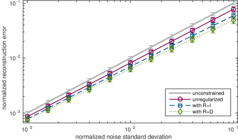
Figure 1: Normalized reconstruction error $\lVert\mathbfit{X}-\mathbfit{X}_{\star}\rVert_{\mathsf{F}}/\lVert\mathbfit{X}_{\star}\rVert$ as a function of the normalized noise level $\sigma/\lVert\mathbfit{X}_{\star}\rVert$. The mean is plotted for the four different solution methods, where $\mathbfit{X}$ is set to $\mathbfit{X}_{\text{U}}$, $\mathbfit{X}_{\text{0}}$, $\mathbfit{X}_{\text{I}}$ and $\mathbfit{X}_{\text{D}}$ for the “unconstrained”, “unregularized”, “with R=I” and “with R=D” cases, respectively. Error bars indicate three standard deviations for each case.

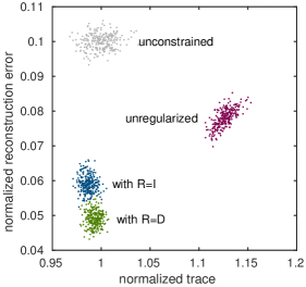
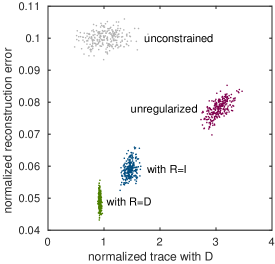
Figure 2: Normalized reconstruction error $\lVert\mathbfit{X}-\mathbfit{X}_{\star}\rVert_{\mathsf{F}}/\lVert\mathbfit{X}_{\star}\rVert$ versus normalized trace $\operatorname{tr}(\mathbfit{X})/\operatorname{tr}(\mathbfit{X}_{\star})$ (left) and $\operatorname{tr}\big{(}\mathbfit{D}^{\mathsf{H}\!}\mathbfit{X}\big{)}/\operatorname{tr}(\mathbfit{D}^{\mathsf{H}\!}\mathbfit{X}_{\star})$ (right) for the four different reconstruction approaches, represented as a scatter plot showing each of the $256$ realizations.

3 Numerical algorithm

We will now briefly review the accelerated proximal gradient (APG) method [6] and then present a novel restart condition for solving (7).

3.1 The accelerated proximal gradient method

Define

(8) $$f(\mathbfit{X})=\tfrac{1}{2}\big{\lVert}\mathscr{A}(\mathbfit{X})-\mathbfit{b}\big{\rVert}_{2}^{2}+\mu\langle\mathbfit{R},\mathbfit{X}\rangle,\quad g(\mathbfit{X})=\iota_{\mathcal{S}_{+}^{N}}(\mathbfit{X})$$

where $\langle\mathbfit{A},\mathbfit{B}\rangle=\operatorname{tr}(\mathbfit{A}^{\mathsf{H}\!}\mathbfit{B})$ is the inner product and $\iota_{\mathcal{S}_{+}^{N}}(\cdot)$ is the indicator function for the set of positive semidefinite Hermitian matrices, i.e., $\iota_{\mathcal{S}_{+}^{N}}(\mathbfit{X})=0$ if $\mathbfit{X}\in\mathcal{S}_{+}^{N}$ and $\iota_{\mathcal{S}_{+}^{N}}(\mathbfit{X})=+\infty$ if $\mathbfit{X}\notin\mathcal{S}_{+}^{N}$. Then, equation (7) is equivalent to the composite convex minimization problem

(9) $$\underset{\mathbfit{X}\in\mathcal{S}^{N}}{\text{minimize}}\ h(\mathbfit{X})=f(\mathbfit{X})+g(\mathbfit{X})\text{.}$$

One representative method to solve (9) is the so-called accelerated proximal gradient (APG) method [6]. Given a function $g$ and $\alpha>0$, define the proximal operator of $g$ as

$$\operatorname{Prox}_{g}^{\alpha}(\mathbfit{X})=\operatorname*{arg\,min}_{\mathbfit{Y}}\bigg{\{}g(\mathbfit{Y})+\tfrac{1}{2\alpha}\lVert\mathbfit{Y}-\mathbfit{X}\rVert^{2}_{\mathsf{F}}\bigg{\}}$$

where $\lVert\cdot\rVert_{\mathsf{F}}$ is the Frobenius norm. Then, the APG method constructs two sequences $\{\mathbfit{X}_{k}\}$ and $\{\mathbfit{Y}_{k}\}$ via the following steps:

(10a) $$t_{k}=\left(\sqrt{4(t_{k-1})^{2}+1}+1\right)/2,$$

(10b) $$\mathbfit{Y}_{k}=\mathbfit{X}_{k}+\tfrac{t_{k-1}-1}{t_{k}}(\mathbfit{X}_{k}-\mathbfit{X}_{k-1}),$$

(10c) $$\mathbfit{X}_{k+1}=\operatorname{Prox}_{g}^{\alpha_{k}}(\mathbfit{Y}_{k}-\alpha_{k}\nabla f(\mathbfit{Y}_{k})),$$

where $t_{0}=1$, $0<\alpha_{k}\leq 1/L$, and $L$ is the maximal eigenvalue of $\mathscr{A}^{\mathsf{H}\!}\mathscr{A}$ with $\mathscr{A}^{\mathsf{H}\!}$ being the adjoint operator for $\mathscr{A}$. With $\mathcal{X}_{\star}$ being the set of minimizers of (9) and $h_{\star}$ being the minimal value, it is well known that the APG method has the following convergence property [6]:

Theorem 3.1.

Let $\mathbfit{X}_{k}$ be the sequence generated by (10a)-(10c) and $\alpha_{k}=1/L,\forall k$. Then for any $k\geq 1$

$$h(\mathbfit{X}_{k})-h_{\star}\leq\frac{2L\operatorname{dist}(\mathbfit{X}_{0},\mathcal{X}_{\star})^{2}}{(k+1)^{2}},$$

where $\operatorname{dist}(\mathbfit{X},\mathcal{X}_{\star})=\inf\{\lVert\mathbfit{X}-\mathbfit{Y}\rVert_{\mathsf{F}}:\mathbfit{Y}\in\mathcal{X}_{\star}\}$.

3.2 The proposed algorithm

Indeed, the attractive $O(1/k^{2})$ convergence rate of the APG method is optimal when solving a convex problem when only first order information is available [29]. However, it has been observed that the objective value (the value of $f$ in this case) sequence generated by the APG method shows oscillations, which slows down convergence speed in practice [32]. To avoid these oscillations, restarting techniques were proposed in [32] wherein $t_{k}$ is reset to $1$ when certain criteria are met. Despite the numerical success of this adaptive restart APG method, it is still unknown whether this method is guaranteed to converge. We therefore propose a new restart criterion that leads to a globally convergent numerical algorithm for solving the trace-regularized coherence retrieval problem (7). Given per-iteration step size $\alpha_{k}>0$, define

(11) $$\mathbfit{Z}_{k+1}=\operatorname{Prox}_{g}^{\alpha_{k}}(\mathbfit{Y}_{k}-\alpha_{k}\nabla f(\mathbfit{Y}_{k})),\quad\mathbfit{U}_{k}=\mathbfit{Y}_{k}-\mathbfit{Z}_{k+1},\quad\mathbfit{V}_{k}=\mathbfit{X}_{k}-\mathbfit{Z}_{k+1}\text{.}$$

When $\mathbfit{X}_{k}\neq\mathbfit{Y}_{k}$, we restart our APG method by setting $t_{k}=1$ if the following does not hold:

(12) $$\langle\mathbfit{U}_{k},\mathbfit{V}_{k}\rangle-\alpha_{k}\langle\mathscr{A}(\mathbfit{U}_{k}),\mathscr{A}(\mathbfit{V}_{k})\rangle\geq\gamma\lVert\mathbfit{V}_{k}\rVert_{\mathsf{F}}^{2}$$

where $\gamma>0$ is a small constant. We note that no extra computation is needed for checking criterion (12) due to the linearity of $\mathscr{A}$ and the necessary quantities having been computed either during step size estimation or in a previous iteration. We summarize our proposed adaptive APG algorithm in Algorithm 1.

Remark 3.2.

$\operatorname{Prox}_{g}^{\alpha}(\mathbfit{X})$ is equal to a projection onto $\mathcal{S}_{+}^{N}$, independent of the value of $\alpha$:

$$\operatorname{Prox}_{g}^{\alpha}(\mathbfit{X})=\operatorname{Proj}_{\mathcal{S}_{+}^{N}}(\mathbfit{X})=\sum_{i=1}^{N}\nolimits\max(\lambda_{i},0)\mathbfit{q}_{i}\mathbfit{q}^{\mathsf{H}\!}_{i}\text{,}$$

where $\left\{\,{\lambda_{i}}\,\right\}_{i}$ and $\left\{\,{\mathbfit{q}_{i}}\,\right\}_{i}$ are the eigenvalues and eigenvectors, respectively, of $\mathbfit{X}$. The gradient of quadratic function $f(\mathbfit{X})$ is equal to:

$$\operatorname{\boldsymbol{\nabla}{}\!}f(\mathbfit{X})=\mathscr{A}^{\mathsf{H}\!}\big{[}\mathscr{A}\left(\mathbfit{X}\right)-\mathbfit{b}\big{]}+\mu\mathbfit{R}^{\mathsf{H}\!}\text{.}$$

In practice, the majority of computation is spent on evaluating $\mathscr{A}$ and $\mathscr{A}^{\mathsf{H}\!}$ as well as the eigenvalue decomposition in the proximal operator. Eigenvalue decomposition scales asymptotically as $\mathcal{O}\left(N^{3}\right)$, whereas evaluating $\mathscr{A}$ and $\mathscr{A}^{\mathsf{H}\!}$ scales as $\mathcal{O}\left(N^{2}M\right)$ in the worst case, with $\mathcal{O}\left(N^{3}\right)$ being the best possible complexity via reduced measurements [14] or exploiting the structure of $\mathscr{A}$ using fast Fourier transforms or separable tensor contractions [37].

Algorithm 1 Adaptive APG algorithm

1:Initialize $\mathbfit{X}_{1}=\mathbfit{Y}_{1}=\mathbfit{Y}_{0}=\mathbfit{X}_{0}$, $t_{1}=1$, $k_{\text{max}},k_{\text{maxres}}\in\mathbb{N}$, $k=1$, $k_{\text{res}}=0$, and $\rho\in(0,1)$

2:while $k\leq k_{\text{max}}$ do

3:     Estimate step size $\alpha_{k}$ using Algorithm 2 and obtain $\mathbfit{Z}_{k+1}=\operatorname{Prox}_{g}^{\alpha_{k}}(\mathbfit{Y}_{k}-\alpha_{k}\operatorname{\boldsymbol{\nabla}{}\!}f(\mathbfit{Y}_{k}))$.

4:     if { $\mathbfit{X}_{k}=\mathbfit{Y}_{k}$ or (12) holds } and $k-k_{\text{res}}\leq k_{\text{maxres}}$  then

5:         Set $\mathbfit{X}_{k+1}=\mathbfit{Z}_{k+1}$.

6:         Set $t_{k+1}=\tfrac{1}{2}\left(\sqrt{4t_{k}^{2}+1}+1\right)$.

7:         Set $\mathbfit{Y}_{k+1}=\mathbfit{X}_{k+1}+\frac{t_{k}-1}{t_{k+1}}(\mathbfit{X}_{k+1}-\mathbfit{X}_{k})$.

8:         Set $k=k+1$.

9:     else

10:         Reset $t_{k}=1$ and update $k_{\text{res}}=k$.

11:         Set $\mathbfit{Y}_{k}=\mathbfit{X}_{k}$.

12:     end if

13:end while

3.2.1 Step size estimation

Setting $\alpha_{k}=1/L$ might be too conservative when the Lipschitz constant $L$ is large. We would like to adaptively choose $\alpha_{k}$ by first initializing with the Barzilai-Borwein (BB) method [5]; our choice of the form with the squared norm in the denominator is motivated by numerical considerations—an inner product is sensitive to cancellation errors and placing it in the denominator can result in numerical instability. After initialization, we then use a standard backtracking technique and adopt the step size $\alpha_{k}$ at $\mathbfit{Y}_{k}$ whenever the following inequality holds:

(13) $$h(\mathbfit{Y}_{k})-h(\mathbfit{Z}_{k+1})\geq\delta\lVert\mathbfit{Y}_{k}-\mathbfit{Z}_{k+1}\rVert_{\mathsf{F}}^{2},$$

where $\delta>0$ is a small constant. It is noted that (13) holds whenever $\alpha_{k}\leq 1/(L+\delta)$ and hence backtracking must terminate. In practice, we find that BB initialization gives a good estimate for the step size and that backtracking is rare. A detailed listing for this step size estimation algorithm is given in Algorithm 2.

Algorithm 2 Estimation of step size $\alpha_{k}$

1:Inputs: $\mathbfit{X}_{k}$, $\mathbfit{Y}_{k}$, $\mathbfit{Y}_{k-1}$, $\operatorname{\boldsymbol{\nabla}{}\!}f(\mathbfit{Y}_{k})$, $\operatorname{\boldsymbol{\nabla}{}\!}f(\mathbfit{Y}_{k-1})$, $\rho<1$ and $\alpha_{\text{min}},\alpha_{\text{max}}>0$.

2:Outputs: Step size $\alpha_{k}$, proximal point $\mathbfit{Z}_{k+1}$

3:if k=1 then

4:     Initialize $\beta=\lVert\mathbfit{b}-\mathscr{A}(\mathbfit{Y}_{k})\rVert_{\mathsf{F}}^{2}/\left\lVert\mathscr{A}^{\mathsf{H}\!}\left[\mathbfit{b}-\mathscr{A}(\mathbfit{Y}_{k})\right]\right\rVert_{\mathsf{F}}^{2}$.

5:else

6:     Calculate $\mathbfit{S}_{k}=\mathbfit{Y}_{k}-\mathbfit{Y}_{k-1}$ and $\mathbfit{T}_{k}=\nabla f(\mathbfit{Y}_{k})-\nabla f(\mathbfit{Y}_{k-1})$.

7:     Initialize $\beta=\lvert\langle\mathbfit{S}_{k},\mathbfit{T}_{k}\rangle\rvert/\lVert\mathbfit{T}_{k}\rVert_{\mathsf{F}}^{2}$.

8:end if

9:for $j=1,2\ldots$ do

10:     Calculate $\mathbfit{Z}_{k+1}=\operatorname{Prox}_{g}^{\beta}\left[\mathbfit{Y}_{k}-\beta\operatorname{\boldsymbol{\nabla}{}\!}f(\mathbfit{Y}_{k})\right]$.

11:     if { $\mathbfit{X}_{k}\neq\mathbfit{Y}_{k}$ and (12) fails to hold } or (13) holds or $\beta<\alpha_{\text{min}}$ then

12:         break

13:     else

14:         Backtrack $\beta=\rho\beta$.

15:     end if

16:end for

17:Set $\alpha_{k}=\min\left[\max(\alpha_{\text{min}},\beta),\alpha_{\text{max}}\right]$.

4 Convergence analysis

In this section, we focus on convergence analysis for Algorithm 1 including an analysis regarding global convergence as well as on the convergence rate. Before proceeding, we first introduce some notation and definitions to be used in the analysis.

4.1 Notation and definitions

Denote $\mathcal{X}_{\star}$ to be the solution set of (7). Given a point $\mathbfit{x}$ and $\epsilon>0$, we define $\mathbb{B}(\mathbfit{x},\epsilon)=\left\{\,{\mathbfit{y}:\lVert\mathbfit{x}-\mathbfit{y}\rVert_{2}\leq\epsilon}\,\right\}$. Given a set $\mathcal{X}$, the relative interior of $\mathcal{X}$, denoted by $\operatorname{ri}(\mathcal{X})$, is defined as

$$\operatorname{ri}(\mathcal{X}):=\left\{\,{\mathbfit{x}\in\mathcal{X}:\exists\epsilon>0,\mathbb{B}(\mathbfit{x},\epsilon)\cap\operatorname{aff}(\mathcal{X})\subseteq\mathcal{X}}\,\right\},$$

where $\operatorname{aff}(\mathcal{X})$ is the affine hull of $\mathcal{X}$. Given a set $\mathcal{X}$ and a member $\mathbfit{x}$, the distance from $\mathbfit{x}$ to $\mathcal{X}$, denoted by $\operatorname{dist}(\mathbfit{x},\mathcal{X})$, is defined as $\operatorname{dist}(\mathbfit{x},\mathcal{X})=\inf\left\{\,{\lVert\mathbfit{x}-\mathbfit{y}\rVert_{2}:\mathbfit{y}\in\mathcal{X}}\,\right\}$. Given a function $f$ and $b\in\mathbb{R}$, we define the sub-level set $\left[f(\mathbfit{x})\leq b\right]$ to be $\left\{\,{\mathbfit{x}:f(\mathbfit{x})\leq b}\,\right\}$. We use $\partial f$ to denote the (limiting) subgradient of $f$.

Let $\mathcal{A}$ and $\mathcal{B}$ be finite dimensional Euclidean spaces and $\Gamma:\mathcal{A}\rightrightarrows\mathcal{B}$ be a set-valued mapping. The graph, domain and inverse of $\Gamma$ are defined by

$$\operatorname{gph}(\Gamma):=\left\{\,{(\mathbfit{u},\mathbfit{v}):\mathbfit{v}\in\Gamma(\mathbfit{u})}\,\right\}\text{, }\operatorname{dom}(\Gamma):=\left\{\,{\mathbfit{u}:\Gamma(\mathbfit{u})\neq\emptyset}\,\right\}\text{, }\Gamma^{-1}(v):=\left\{\,{\mathbfit{u}:\Gamma(\mathbfit{u})=\mathbfit{v}}\,\right\}.$$

In the following context, we define a useful property for set-valueed mappings.

Definition 4.1.

A set-valued mapping $\Gamma:\mathcal{A}\rightrightarrows\mathcal{B}$ is said to be metrically subregular at $\mathbfit{\bar{x}}\in\mathcal{A}$ for $\mathbfit{\bar{y}}\in\mathcal{B}$ if $(\mathbfit{\bar{x}},\mathbfit{\bar{y}})\in\operatorname{gph}(\Gamma)$ and there exist $\kappa,\epsilon>0$ such that

(14) $$\operatorname{dist}(\mathbfit{x},\Gamma^{-1}(\mathbfit{\bar{y}}))\leq\kappa\operatorname{dist}(\mathbfit{\bar{y}},\Gamma(\mathbfit{x})),\ \forall\mathbfit{x}\in\mathbb{B}(\mathbfit{\bar{x}},\epsilon).$$

4.2 Global convergence

We first show that Algorithm 1 converges to a global minimum, provided the generated sequence is bounded.

Theorem 4.2.

Let $\{\mathbfit{X}_{k}\}$ be the sequence generated by Algorithm 1. If $\{\mathbfit{X}_{k}\}$ is bounded, then $\{\mathbfit{X}_{k}\}$ converges to a global minimum of (7), denoted as $\mathbfit{\bar{X}}$.

Proof 4.3.

See Appendix A.

Remark 4.4.

The proof is based on the recently established Kurdyka-Łojasiewicz (KL) property [2, 8], which provides a framework for typical descent algorithms whose generated sequences are bounded. However, the boundedness condition might not hold for semidefinite programming problems such as (7).

In coherence retrieval, we will show that the boundedness condition on $\{\mathbfit{X}_{k}\}$ holds when the measurement operator $\mathscr{A}$ satisfies a certain mild condition. Let $\mathbfit{A}=(\mathbfit{\hat{K}}_{1},\ldots,\mathbfit{\hat{K}}_{M})^{\mathsf{H}\!}\in{\mathbb{C}}^{{MN}\times{N}}$ where the $\mathbfit{\hat{K}}_{m}\text{s}\in{\mathbb{C}}^{{N}\times{N}}$ are such that $\mathbfit{K}_{m}=\mathbfit{\hat{K}}_{m}\mathbfit{\hat{K}}^{\mathsf{H}\!}_{m}$ for all $m\in\left\{\,{1,\ldots,M}\,\right\}$. We make the following assumption on $\mathbfit{A}$:

Assumption 4.1.

The matrix $\mathbfit{A}$ has full column rank.

In practice, 4.1 always holds because either the measurements are designed to ensure $\mathbfit{A}$ is full rank, or a smaller set of basis functions are used to remove the ambiguity, e.g., we can choose a larger sampling interval in the case of $\operatorname{sinc}$ basis functions, or we can use the nonzero right singular vectors of $\mathbfit{A}$ to set a new basis based on our original basis.

Proposition 4.5.

Let $\{\mathbfit{X}_{k}\}$ to be the sequence generated by Algorithm 1. Suppose 4.1 holds. Then, $\{\mathbfit{X}_{k}\}$ is bounded.

Proof 4.6.

See Appendix B.

Combining Theorem 4.2 and Proposition 4.5, we obtain that Algorithm 1 is globally convergent under 4.1.

Corollary 4.7.

Let $\{\mathbfit{X}_{k}\}$ to be the sequence generated by Algorithm 1. Suppose 4.1 holds. Then, $\{\mathbfit{X}_{k}\}$ converges to a global minimum of (7), denoted as $\mathbfit{\bar{X}}$.

4.3 Convergence rate analysis

In this section, we first impose a reasonable condition on the solution set $\mathcal{X}_{\star}$. Using this condition, we prove that Algorithm 1 converges linearly.

Assumption 4.2.

We make the following assumptions on $\mathcal{X}_{\star}$: a) $\mathcal{X}_{\star}\neq\emptyset$. b) There exists an $\mathbfit{X}_{\star}\in\mathcal{X}_{\star}$ satisfying

(15) $$\mathbf{0}\in\operatorname{\boldsymbol{\nabla}{}\!}f(\mathbfit{X}_{\star})+\operatorname{ri}\left(\mathcal{N}_{\mathcal{S}_{+}^{N}}(\mathbfit{X}_{\star})\right)$$

where $\mathcal{N}_{\mathcal{S}_{+}^{N}}(\mathbfit{X})$ denotes the normal cone of $\mathcal{S}_{+}^{N}$ at $\mathbfit{X}$.

Remark 4.8.

The first order optimality condition of $h$ implies

(16) $$0\in\operatorname{\boldsymbol{\nabla}{}\!}f(\mathbfit{X})+\mathcal{N}_{\mathcal{S}_{+}^{N}}(\mathbfit{X}),\ \forall\mathbfit{X}\in\mathcal{X}_{\star}.$$

Condition (15) is slightly more restrictive than (16), but (15) only needs to hold at one point of $\mathcal{X}_{\star}$. Moreover, from the proof of Proposition 4.9, one sufficient condition for ensuring (15) is that there exists some $\mathbfit{X}_{\star}\in\mathcal{X}_{\star}$ such that $\operatorname{rank}(\mathbfit{X}_{\star})=N$, i.e., $\mathbfit{X}_{\star}$ is full rank.

Based on recent work [16], we ensure $\partial h$ is metrically sub-regular at any $\bar{\mathbfit{X}}\in\mathcal{X}_{\star}$ for $\mathbf{0}$ in the next proposition.

Proposition 4.9.

Let $h=f+g$ be defined in (8). Suppose 4.2 holds. Then, for any $\bar{\mathbfit{X}}\in\mathcal{X}_{\star}$, $\partial h$ is metrically sub-regular at $\bar{\mathbfit{X}}$ for $0$.

Proof 4.10.

See Appendix C.

Remark 4.11.

Proposition 3.2 in [16] is a characterization of metric sub-regularity for real symmetric positive semidefinite matrices. However, the analysis in [16] can easily be extended for Hermitian positive semidefinite matrices over $\mathbb{R}$.

Now, we can establish local linear convergence for Algorithm 1 via the following:

Theorem 4.12.

Let $h=f+g$ be defined in (8) and the sequence $\{\mathbfit{X}_{k}\}$ be generated by Algorithm 1. Suppose 4.1 and 4.2 holds. Then, there exists some $\bar{\mathbfit{X}}\in\mathcal{X}_{\star}$ such that one of the following assertions holds:
1. $\left\{\,{\mathbfit{X}_{k}}\,\right\}$ converges to $\bar{\mathbfit{X}}$ in finite steps.
2. $\left\{\,{h(\mathbfit{X}_{k})}\,\right\}$ and $\left\{\,{\mathbfit{X}_{k}}\,\right\}$ linearly converge to $h(\bar{\mathbfit{X}})$ and $\bar{\mathbfit{X}}$, respectively, i.e., there exist $c_{1},c_{2}>0$, $w_{1},w_{2}\in(0,1)$ and $k_{\ell}>0$ such that

$$h(\mathbfit{X}_{k})-h(\bar{\mathbfit{X}})\leq c_{1}w_{1}^{k}\text{, and }\lVert\mathbfit{X}_{k}-\bar{\mathbfit{X}}\rVert_{\mathsf{F}}\leq c_{2}w_{2}^{k},\ \forall k>k_{\ell}.$$

Proof 4.13.

See Appendix D.

5 Results

We now apply our algorithm to two data sets from translation-only one-dimensional phase-space tomography [35, 44]. One is a simulation with realistic noise of two coherent Gaussian beams that are slightly decohered with respect to each other. Another is experimental data from [49] consisting of a Schell-model source imaged by a single positive lens. In both cases, the data consists of intensity profiles captured at $250\text{\,}\mathrm{\SIUnitSymbolMicro m}$ axial intervals by a single row of pixels in a $3.2\text{\,}\mathrm{\SIUnitSymbolMicro m}$ pitch camera with wavelength $\lambda$ equal to $532\text{\,}\mathrm{nm}$.

While our approach can be applied to more complicated tomographic apparatuses [27, 26] as long as the amplitude transfer function $K(\mathbfit{p},\mathbfit{q}_{m})$ is known, we focus on the translation-only one-dimensional phase-space tomography example as it is well-studied and a good base from which to extrapolate insights.

With one-dimensional phase-space tomography, the optical field as well as the mutual intensity are assumed to be constant along one of the spatial axes, i.e., $U(\mathbfit{p})$ can be written as a one-dimensional function $U(x)$, being constant along $y$, and thus $J(\mathbfit{p}_{1},\mathbfit{p}_{2})$ can also be written as $J(x_{1},x_{2})$. We assume that the optical field can be Nyquist sampled at intervals of $\Delta$ and has negligible energy when $\lvert x\rvert>N\Delta/2$. Thus, we employ the following $\operatorname{sinc}$ basis functions:

$$\xi_{n}(x)=\sqrt{\Delta}\sin\big{[}\pi(x/\Delta-n+n_{0})\big{]}\big{/}\big{[}\pi(x/\Delta-n+n_{0})\big{]}$$

where $n=1,\dots,N$ and $n_{0}=(N+1)/2$.

For translation-only one-dimensional phase-space tomography, the light from the source propagates through free space towards the measurement points $\mathbfit{r}_{m}$, each of which can be fully specified by transverse position $x_{m}$ and axial position $z_{m}$; a camera sensor is translated to the various axial positions and intensity measurements are obtained from the pixel values in a single row. We assume $\Delta\gg\lambda$ and thus use the Fresnel diffraction integral to compute the forward model $\mathbfit{k}_{m}$s and thus the measurement operators $\mathbfit{K}_{m}$s:

$$\mathbfit{k}_{m}[n] =\int\xi_{n}(x)\exp\left[\frac{\mathrm{i}2\pi}{\lambda z_{m}}(x_{m}-x)^{2}\right]\Big{/}\sqrt{\mathrm{i}\lambda z_{m}}\mathop{\mathrm{d}x}$$

$$=\frac{\exp\left(\alpha_{m,n}\right)}{2\sqrt{\mathrm{i}\lambda z_{m}/\Delta}}\left\{\operatorname{erf}\left[-\sqrt{\alpha_{m,n}}+\frac{\sqrt{\mathrm{i}\pi\lambda z_{m}}}{2\Delta}\right]-\operatorname{erf}\left[-\sqrt{\alpha_{m,n}}-\frac{\sqrt{\mathrm{i}\pi\lambda z_{m}}}{2\Delta}\right]\right\},$$

where $\mathrm{i}$ is the imaginary constant, $\sqrt{\mathrm{i}}=(1+\mathrm{i})/\sqrt{2}$, $\operatorname{erf}(\zeta)=\tfrac{2}{\sqrt{\pi}}\int_{0}^{\zeta}\exp(-t^{2})\mathop{\mathrm{d}t}$ is the error function, and $\alpha_{m,n}=\mathrm{i}\pi(x_{m}-n\Delta)^{2}/(\lambda z_{m})$. Since these $\mathbfit{k}_{m}$s are deterministic, $\mathbfit{K}_{m}=\mathbfit{k}^{\mathsf{T}\!}_{m}\mathbfit{k}_{m}$.

The constant parameters we chose for our numerical algorithm were:

$$\mathbfit{X}_{0}=\mathbf{0} \delta=10^{-8} \gamma=10^{-5} \rho=\tfrac{1}{2}$$

$$\alpha_{\text{min}}=10^{-8} \alpha_{\text{max}}=10^{8} k_{\text{max}}=1000 k_{\text{maxres}}=250$$

For comparison, we also run standard proximal gradients (PG), accelerated proximal gradients (APG) and adaptive restart accelerated proximal gradients (restart APG) using publicly available code accompanying [32]. For instrumentation, we added code to the official source code in order to record the time taken and acceleration parameter at each iteration. Furthermore, each algorithm was run a second time wherein the value of $\mathbfit{X}$ at each iteration was recorded in order to compute the value of the merit function at each iteration. All computations were performed using MATLAB running on an Intel Xeon E5-2630 CPU.

5.1 Simulated Data

We simulate a mostly coherent sum of two parallel Gaussian beams with coplanar waists, as given by the following mutual intensity function:

$$J(x_{1},x_{2}) =G(x_{1};x_{0})G(x_{2};x_{0})+G(x_{1};-x_{0})G(x_{2};-x_{0})$$

$$\quad+\chi\big{[}G(x_{1};x_{0})G(x_{2};-x_{0})+G(x_{1};-x_{0})G(x_{2};x_{0})\big{]}$$

where $G(x;a)=\exp\left[-(x-a)^{2}/(2\sigma^{2})\right]$, $x_{0}=$64\text{\,}\mathrm{\SIUnitSymbolMicro m}$$, $\sigma=$32\text{\,}\mathrm{\SIUnitSymbolMicro m}$$ and $\chi=0.9$. This partially coherent field, discretized into a $51\text{\times}51$ mutual intensity matrix ($N=51$) using a sampling interval of $\Delta=$6.4\text{\,}\mathrm{\SIUnitSymbolMicro m}$$, is then propagated to $201$ axial positions spaced $250\text{\,}\mathrm{\SIUnitSymbolMicro m}$ apart. For each axial position, we consider $101$ intensity point samples spaced $3.2\text{\,}\mathrm{\SIUnitSymbolMicro m}$ apart for the measurements. This set of true intensities is shown in Figure 3 under the heading ``noiseless''. The smallest and largest singular values of matrix $\mathbfit{A}$ as it is defined in Section 4.2 were $a_{\text{min}}=3.094$ and $a_{\text{max}}=7.925$, respectively.

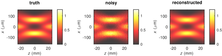
Figure 3: Noisy measurements of the intensity are shown on left, with the true intensity shown on right. Propagated intensity of a regularized reconstructed result is shown in center. In all images, light propagates from left to right, and the intensity is in arbitrary units.

To emulate real world conditions where the $\sigma_{m}$s are unknown, we simulate collecting $16$ measurements for each intensity point sample, with their mean treated as the $y_{m}$s in our model and the standard deviation across these $16$ samples used as an approximation to $\sigma_{m}\sqrt{16}$. The noisy data for each measurement is generated by first drawing from a Poisson distribution whose rate parameter is proportional to the true intensity at that point, with the sum of all the rate parameters made to equal $1.02\text{\times}{10}^{5}\text{\,}\mathrm{p}$hotons. We then add Gaussian noise with standard deviation equal to $0.01$ times the maximum of all the rate parameters; this is to simulate readout and quantization noise that would be typically expected of an 8-bit sensor. This set of simulated measurements is shown in Figure 3 under the heading ``noisy''. We then run our algorithm with the following inputs:

• noiseless: The $y_{m}$s are set to the ideal noiseless intensity, with the $\sigma_{m}$s set to $1$ and $\mu=0$ (i.e., no regularization).

• unregularized: The $y_{m}$s and $\sigma_{m}$s are set to our simulated noisy data, with $\mu=0$ (i.e., no regularization).

• nuclear: This uses the simulated noisy data and $\mathbfit{R}=\mathbfit{I}$ (i.e., nuclear norm regularization). $\mu$ is set such that $\tfrac{1}{2}\lVert\mathscr{A}(\mathbfit{X})-\mathbfit{b}\rVert_{2}^{2}\approx\alpha M/2$ upon convergence. The $\alpha M/2$ threshold for $\tfrac{1}{2}\lVert\mathscr{A}(\mathbfit{X})-\mathbfit{b}\rVert_{2}^{2}$ arises from the fact that the norm-squared expression follows a chi-squared distribution with $M$ degrees of freedom assuming that the $\sigma_{m}$s are correct values for the standard deviations of the Gaussian noise. $M/2$ would be the mean for such a distribution, and $\alpha$ is used to adjust the threshold to take into account how well estimated the $\sigma_{m}$s are and how much of the distribution we want to include. For this particular set of data, we are fairly confident of our estimates of $\sigma_{m}$ and have thus set $\alpha=1.5$.

• gradient: This uses the simulated noisy data and $\mathbfit{R}=\mathbfit{D}$, a tridiagonal matrix with all the elements in the diagonal equal to $1$ and all the off-diagonal elements equal to $-\tfrac{1}{2}$. $\mu$ is set such that $\tfrac{1}{2}\lVert\mathscr{A}(\mathbfit{X})-\mathbfit{b}\rVert_{2}^{2}\approx\alpha M/2$ upon convergence. The penalty term $\operatorname{tr}(\mathbfit{D}^{\mathsf{H}\!}\mathbfit{X})$ is thus equivalent to applying a Haar wavelet to both the rows and columns of $\mathbfit{X}$, keeping only the high frequency components and then taking the trace. The application of $\mathbfit{D}$ is a simple approximation for a derivative operator on $x_{1}$ and $x_{2}$ in the continuous domain, and it physically corresponds to a desire to reduce the energy present in the first order spatial derivative of the optical wave function. Mathematically, it penalizes nonsmooth solutions to our problem, and it is motivated by our a priori knowledge that the true solution is smooth.

• early stop: This is the same as the unregularized case, except we terminate our algorithm when $\tfrac{1}{2}\lVert\mathscr{A}(\mathbfit{X})-\mathbfit{b}\rVert_{2}^{2}$ drops below $\alpha M/2$ where $\alpha=1.5$. This result is used as a point of reference for comparison with the regularized results, since these results all have approximately the same level of measurement mismatch, and therefore the differences are due to the presence of and choice of regularizer.

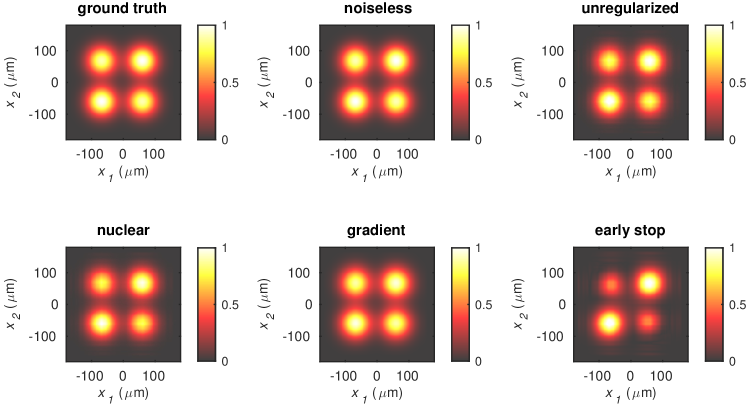
Figure 4: Magnitude of the mutual intensity functions for the simulated data. They are all drawn using the same scale, normalized to the maximum magnitude of the ground truth.

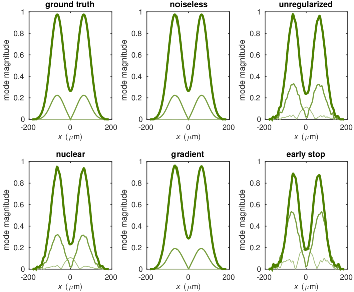
Figure 5: Amplitude plots of the $3$ highest energy coherent modes for each mutual intensity function.

	noiseless	unregularized	nuclear	gradient	early stop
normalized error	$7.524\text{\times}{10}^{-5}$	$0.1147$	$0.1438$	$0.039\,79$	$0.3977$
trace distance	$6.103\text{\times}{10}^{-5}$	$0.079\,08$	$0.076\,58$	$0.025\,34$	$0.2887$

Table 1: Quantitative measurements of error for the different reconstructed mutual intensity matrices. The normalized error is defined as $\lVert\mathbfit{X}-\mathbfit{X}_{\text{true}}\rVert_{\mathsf{F}}/\lVert\mathbfit{X}_{\text{true}}\rVert_{\mathsf{F}}$. The trace distance, a quantity used to describe the difference between two quantum states, is equal to half the sum of the singular values of $\rho-\rho_{\text{true}}$, where $\rho$ and $\rho_{\text{true}}$ are equal to $\mathbfit{X}/\operatorname{tr}(\mathbfit{X})$ and $\mathbfit{X}_{\text{true}}/\operatorname{tr}(\mathbfit{X}_{\text{true}})$ respectively.

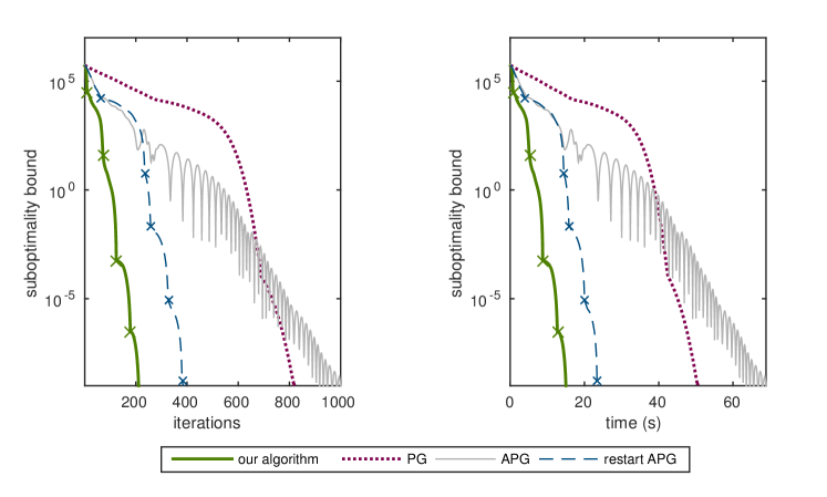
Figure 6: Comparison of convergence across different algorithms for the simulated data. The vertical axis is the difference between the value of $f(\mathbfit{X})$ and the lowest attained value of $f(\mathbfit{X})$ across all algorithms, which in turn gives an upper bound on the suboptimality. On left, the horizontal axis is the number of iterations. On right, the horizontal axis is time taken. The $\times$s mark where restarts occurred.

The magnitude of the reconstructed mutual intensity functions are shown in Figure 4, and the magnitude of their coherent modes [48] are given in Figure 5. The propagated intensity using the gradient result is shown in Figure 3. Since the ground truth is known, we give a summary of the reconstruction error using various metrics in Table 1. A convergence comparison between algorithms for the gradient input is shown in Figure 6.

As is evident from the results, especially Figure 5, noise introduces additional energy (as seen in the increased amplitude for the second mode) as well as an additional mode, resulting in a reconstructed mutual intensity that appears less coherent than the ground truth. Furthermore, noise also induces additional high frequency content in the reconstructed result. For the specific value of $\alpha$ used, regularization using the nuclear norm only yields marginal improvements over the unregularized reconstruction, whereas regularization using the smoothness-inducing regularizer both smooths the result and reduces the number of significant modes back down to the correct number of modes. Of course, we can increase the $\mu$ parameter for the nuclear norm case to reduce the number of modes, but it does not fully smooth the result and results in a mutual intensity that does not match the measurements as well as the smooth-prior regularized result. We note that the early stop result has the same amount of measurement mismatch as the two regularized solutions, showing how ill-posed the problem is and the necessity for regularization.

Our algorithm also converges faster than the three other methods given in Figure 6, albeit restart APG converges asymptotically as fast. Non-restarting APG oscillates due to excess critical momentum, as described in [32]. The advantages of our algorithm are that: (1) it is provably convergent, whereas to the best of our knowledge no proof of convergence has been given for the algorithm given in [32], and (2) it converges much faster than the provably convergent non-restarting APG (i.e., FISTA [6]).

5.2 Experimental Data

We use the experimental data from [49], wherein the intensity profile of a partially coherent beam is imaged at $201$ positions along the optical axis. The partially coherent beam was generated by focusing an LED light source through a $532\text{\,}\mathrm{nm}$ bandpass filter onto a $100\text{\,}\mathrm{\SIUnitSymbolMicro m}$ slit located at the front focal plane of a $100\text{\,}\mathrm{mm}$ focal length cylindrical lens. A $500\text{\,}\mathrm{\SIUnitSymbolMicro m}$ slit placed at the back focal plane is illuminated by light passing through the cylindrical lens, and this slit is imaged using a $50\text{\,}\mathrm{mm}$ cylindrical lens placed $150\text{\,}\mathrm{mm}$ after the slit. Based on visual inspection, the axial positions captured were located between $z=$-30.25\text{\,}\mathrm{mm}$$ and $z=$19.75\text{\,}\mathrm{mm}$$ relative to the image of the slit.

The experimental data $y_{m}$s are taken from a single row on a camera with $3.2\text{\,}\mathrm{\SIUnitSymbolMicro m}$ pitch, and the standard deviation $\sigma_{m}$s were estimated from the neighboring $16$ rows. A visualization of the measured and theoretical intensities are shown in Figure 7. We use a $\operatorname{sinc}$ basis with sampling interval $\Delta=$6.4\text{\,}\mathrm{\SIUnitSymbolMicro m}$$ to discretize the mutual intensity into a $101\text{\times}101$ matrix ($N=101$). We note that the field does not necessarily have a spatial band-limit compatible with the sampling interval, but since we only measure the intensity at intervals of $3.2\text{\,}\mathrm{\SIUnitSymbolMicro m}$, it would be very difficult to recover any information at a higher sampling rate and hence we ignore the higher frequency components. The smallest and largest singular values of the matrix $\mathbfit{A}$ as it is defined in Section 4.2 were $a_{\text{min}}=7.625$ and $a_{\text{max}}=14.18$.

An aberration-free theoretical estimate of the mutual intensity is:

$$J(x_{1},x_{2}) \propto\operatorname{rect}(\beta_{1}x_{1})\operatorname{rect}(\beta_{1}x_{2})\operatorname{sinc}\big{[}\beta_{2}(x_{1}-x_{2})\big{]}\exp\big{[}\mathrm{i}\beta_{3}(x_{1}^{2}-x_{2}^{2})\big{]}$$

$$\quad\otimes\operatorname{sinc}(x_{1}/\Delta)\operatorname{sinc}(x_{2}/\Delta)$$

where $\beta_{1}=$4\text{\,}{\mathrm{mm}}^{-1}$$, $\beta_{2}^{-1}=$532\text{\,}\mathrm{\SIUnitSymbolMicro m}$$, $\beta_{3}=$1.9684\text{\times}{10}^{-4}\text{\,}{\mathrm{\SIUnitSymbolMicro m}}^{-2}$$, and $\otimes$ denotes convolution. Since ground truth is not available, we use this aberration-free estimate as a rough point of reference; it is not intended to be interpreted as the ground truth, which may be slightly blurred or distorted by aberrations.

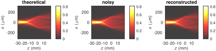
Figure 7: Noisy measurements of the intensity are shown on left, with the theoretical aberration-free intensity profile shown on the right. Propagated intensity of a regularized reconstructed result is shown in center. In all images, light propagates from left to right, and the intensity is in arbitrary units. The theoretical intensity is provided as a point of reference and is not necessarily the ground truth.

We again use several different sets of parameters for our algorithm, although we replaced two of the input sets and used a different value of $\alpha$ for the target value of $\tfrac{1}{2}\lVert\mathscr{A}(\mathbfit{X})-\mathbfit{b}\rVert_{2}^{2}$ in the regularized reconstructions. Instead of the early stop and noiseless input parameter sets, we added the nuclear+support and window input parameter sets. The former uses the same regularizer as the nuclear data set, but additionally forces coefficients of basis functions whose centers lie outside the center $250\text{\,}\mathrm{\SIUnitSymbolMicro m}$ region to be zero, as a way to demonstrate the state of the art nuclear norm regularizer combined with a hard support constraint. The window input parameter set uses $\mathbfit{R}=\mathbfit{W}$, a diagonal matrix whose entries are unity in the center $250\text{\,}\mathrm{\SIUnitSymbolMicro m}$ region and increase linearly away from this region, up to a maximum of $391$ at the ends. The idea with these additional input sets is to demonstrate how one can incorporate a priori information about the support of the solution—since we know our slit should be imaged to a region that wide, we would like to penalize any contributions outside of this region. While nuclear+support uses a hard constraint, it is not necessarily appropriate because the field may not actually be exactly zero outside the region, due to the presence of possible aberrations in the system. The window approach is a gentler way of finding a less energetic solution while at the same time preferring to remove energy from areas where we do not expect much energy to be present, i.e., it is a soft support constraint. Coincidentally, this regularizer is also equivalent to imposing a smoothness constraint on the intensity in the far field of the partially coherent beam. We also chose a value of $\alpha=5$ to account for additional possible errors in $\mathscr{A}$ (due to imperfect equipment and calibration) and standard deviation estimation.

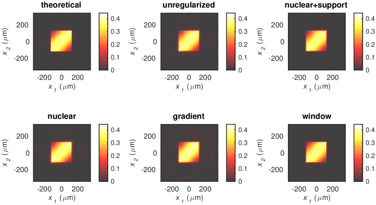
Figure 8: Magnitude of the mutual intensity functions for the experimental data. They are all drawn using the same scale, with values in arbitrary units.

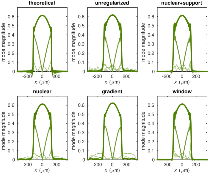
Figure 9: Magnitude plots of the $4$ highest energy coherent modes for each mutual intensity function.

	unregularized	nuclear+support	nuclear	gradient	window
normalized RMSE	$0.2363$	$0.2336$	$0.2317$	$0.2189$	$0.2176$
trace distance	$0.1795$	$0.1717$	$0.1666$	$0.1743$	$0.1486$

Table 2: Quantitative measurements of the difference between the mutual intensity matrices reconstructed from experimental data and the aberration-free mutual intensity estimate. The quantities are defined in the same way as Table 1, with the aberration-free mutual intensity estimate taken as the ``truth''.

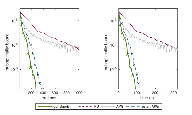
Figure 10: Comparison of convergence across different algorithms for the experimental data. The vertical axis is the difference between the value of $f(\mathbfit{X})$ and the lowest attained value of $f(\mathbfit{X})$ across all algorithms, which in turn gives an upper bound on the suboptimality. On left, the horizontal axis is the number of iterations. On right, the horizontal axis is time taken. The $\times$s mark where restarts occurred.

The reconstructed mutual intensity functions are shown in Figure 8 with modes shown in Figure 9. We give quantitative comparisons between the theoretical mutual intensity and the reconstructed mutual intensity in Table 2, and a comparison of algorithm convergence for the window input set is given in Figure 10. All regularized solutions remove some amount of noise, as evident in the increased smoothness and reduction of high order mode energy in the coherent modes visualization. The nuclear result cleans up the reconstruction compared to the noisy reconstruction, but it still leaves a lot of excess energy in the higher order modes, especially energy outside the region occupied by the slit. The gradient regularizer is good at reducing the number of modes, but it oversmoothes the result—the third mode spills outside of the region occupied by the slit and resembles neither the third mode from the theoretical results nor that of the noisy results, and the sharp edges of the second mode are gone. The image of the magnitude of the mutual intensity in Figure 8 is also quite blurry. While the nuclear result is an improvement over the unregularized result, it is obvious that applying additional prior information about the support yields a much better reconstruction, as can be seen in the nuclear+support and window cases. However, the application of a hard support constraint might not be suitable in this particular situation, as we do not know about the extent of aberrations in the imaging system. Furthermore, window does manage to reconstruct the third mode better than all of the other methods; nuclear+support still does not perform as well, and leaves excess energy in the fourth mode.

The experimental data convergence results in Figure 10 are quite similar to the one for the simulated data—our algorithm has an asymptotic convergence rate comparable to gradient restart APG, albeit we again reach the fast convergence regime faster.

6 Conclusion

We have demonstrated that trace-regularized coherence retrieval can be a powerful tool in recovering the mutual intensity when the inverse problem is ill-conditioned. The generalization of the nuclear-norm enables flexibility in applying a priori information, leading to higher quality reconstructions. Furthermore, we have demonstrated an efficient numerical scheme for our coherence retrieval model, with performance at worst comparable to the state-of-the-art adaptive restart APG scheme while simultaneously being provably globally convergent, with mild conditions required for linear convergence.

This work uses very simple $\mathbfit{R}$ matrices for regularization, with good results, but more flexibility and power can be attained by leveraging the framework of tight frames through further study. Furthermore, a method for exploiting redundant information in the measurements to calibrate real-world $\mathbfit{K}_{m}$s as well as methods to reduce the memory and computational footprint for high dimensional structured mutual intensity matrices are all potential avenues for future exploration.

Appendix A Proof of Theorem 4.2

Given $\eta\in(0,+\infty]$, define $\Phi_{\eta}$ be the class of all concave and continuous functions $\phi:[0,\eta)\rightarrow\mathbb{R}_{+}$ that satisfy $\phi(0)=0$, $\phi$ is $C^{1}$ on $(0,\eta)$ and continuous at $0$, and $\phi^{{}^{\prime}}(s)>0,\ \forall s\in(0,\eta)$.

Definition A.1.

Let $f:\mathbb{R}^{n}\rightarrow(-\infty,+\infty]$ be proper and lower semicontinuous. The function $f$ is said to satisfy the Kurdyka-Łojasiewicz (KL) inequality at $\mathbfit{\bar{x}}\in\operatorname{dom}(\partial f)$ if there exist $\eta\in(0,+\infty]$, a neighborhood $\mathcal{U}$ of $\mathbfit{\bar{x}}$ and a function $\phi\in\Phi_{\eta}$, such that for all $\mathbfit{x}\in\mathcal{U}\cap\left[f(\mathbfit{\bar{x}})<f(\mathbfit{x})<f(\mathbfit{\bar{x}})+\eta\right]$, the following inequality holds:

(17) $$\phi^{{}^{\prime}}(f(\mathbfit{x})-f(\mathbfit{\bar{x}}))\operatorname{dist}(\mathbf{0},\partial f(\mathbfit{x}))\geq 1.$$

A function $f(\mathbfit{x})$ is called a KL function if $f$ satisfies the KL property at every $\mathbfit{x}\in\operatorname{dom}(\partial f)$.

We will now show some basic properties of Algorithm 1 in the following lemmas and use them to prove the global convergence of Algorithm 1.

Lemma A.2.

Let $\{\mathbfit{X}_{k}\}$ be the sequence generated by Algorithm 1. Then, there exists $a,b>0$ and $\bar{w}\in[0,1)$ such that for all $k\geq 0$, we have

(18) $$h(\mathbfit{X}_{k})-h(\mathbfit{X}_{k+1}) \geq a\lVert\mathbfit{X}_{k}-\mathbfit{X}_{k+1}\rVert_{\mathsf{F}}^{2},$$

(19) $${\operatorname{dist}}(0,\partial h(\mathbfit{X}_{k+1})) \leq b\left(\lVert\mathbfit{X}_{k+1}-\mathbfit{X}_{k}\rVert_{\mathsf{F}}+\bar{w}\lVert\mathbfit{X}_{k}-\mathbfit{X}_{k-1}\rVert_{\mathsf{F}}\right).$$

Proof A.3.

Define

(20) $$\mathbfit{W}_{k+1}=\operatorname{Prox}_{g}^{\alpha_{k}}(\mathbfit{X}_{k}-\alpha_{k}\operatorname{\boldsymbol{\nabla}{}\!}f(\mathbfit{X}_{k})).$$

Let $\Omega_{1}=\left\{\,{k:\mathbfit{X}_{k+1}=\mathbfit{W}_{k+1},k>1}\,\right\}$ and $\Omega_{2}=\left\{\,{k:\mathbfit{X}_{k+1}=\mathbfit{Z}_{k+1}}\,\right\}$ where $\mathbfit{Z}_{k+1}$ is defined in (11). Then, $\Omega_{1}\cap\Omega_{2}=\emptyset$ and $\Omega_{1}\cup\Omega_{2}=\mathbb{N}$. We consider two cases: (I) $k\in\Omega_{1}$ and (II) $k\in\Omega_{2}$.

Case I. $k\in\Omega_{1}$ implies that $\mathbfit{X}_{k}=\mathbfit{Y}_{k}$, and hence $h(\mathbfit{X}_{k})-h(\mathbfit{X}_{k+1})\geq\delta\lVert\mathbfit{X}_{k}-\mathbfit{X}_{k+1}\rVert_{\mathsf{F}}^{2}$ due to inequality (13) from the step size estimation process. From the optimality condition of (20), we know

(21) $$\tfrac{1}{\alpha_{k}}(\mathbfit{X}_{k}-\mathbfit{X}_{k+1})-\operatorname{\boldsymbol{\nabla}{}\!}f(\mathbfit{X}_{k})\in\partial g(\mathbfit{X}_{k+1}).$$

The inequality (21) implies

$$\operatorname{dist}(0,\partial h(\mathbfit{X}_{k+1})) \leq\left\lVert\operatorname{\boldsymbol{\nabla}{}\!}f(\mathbfit{X}_{k+1})+\tfrac{1}{\alpha_{k}}(\mathbfit{X}_{k}-\mathbfit{X}_{k+1})-\operatorname{\boldsymbol{\nabla}{}\!}f(\mathbfit{X}_{k})\right\rVert_{\mathsf{F}}$$

$$\leq(L+1/\alpha_{\text{min}})\lVert\mathbfit{X}_{k+1}-\mathbfit{X}_{k}\rVert_{\mathsf{F}}.$$

since $\alpha_{k}\geq\alpha_{\text{min}}>0,\forall k$.
Case II: $k\in\Omega_{2}$. From the first order optimality condition of (11), we have

(22) $$\tfrac{1}{\alpha_{k}}(\mathbfit{Y}_{k}-\mathbfit{Z}_{k+1})-\operatorname{\boldsymbol{\nabla}{}\!}f(\mathbfit{Y}_{k})\in\partial g(\mathbfit{Z}_{k+1}).$$

Then, together with the convexity of $h$ and the fact that $\mathbfit{X}_{k+1}=\mathbfit{Z}_{k+1}$, we have

$$h(\mathbfit{X}_{k})-h(\mathbfit{X}_{k+1}) \geq\left\langle\operatorname{\boldsymbol{\nabla}{}\!}f(\mathbfit{Z}_{k+1})+\tfrac{1}{\alpha_{k}}(\mathbfit{Y}_{k}-\mathbfit{Z}_{k+1})-\operatorname{\boldsymbol{\nabla}{}\!}f(\mathbfit{Y}_{k}),\mathbfit{X}_{k}-\mathbfit{Z}_{k+1}\right\rangle$$

$$=\left\langle\left(\tfrac{1}{\alpha_{k}}\mathbf{I}-\mathscr{A}^{\mathsf{H}\!}\mathscr{A}\right)(\mathbfit{Y}_{k}-\mathbfit{Z}_{k+1}),\mathbfit{X}_{k}-\mathbfit{Z}_{k+1}\right\rangle$$

$$\geq\frac{\gamma}{\alpha_{\text{max}}}\lVert\mathbfit{X}_{k}-\mathbfit{X}_{k+1}\rVert_{\mathsf{F}}^{2},$$

since the inequality (12) holds and $0<\alpha_{\text{min}}\leq\alpha_{k}\leq\alpha_{\text{max}}$. Moreover, the inequality

$$\begin{split}\operatorname{dist}\left(0,\partial h(\mathbfit{X}_{k+1})\right)&\leq\left\lVert\operatorname{\boldsymbol{\nabla}{}\!}f(\mathbfit{Z}_{k+1})+\tfrac{1}{\alpha_{k}}(\mathbfit{Y}_{k}-\mathbfit{Z}_{k+1})-\operatorname{\boldsymbol{\nabla}{}\!}f(\mathbfit{Y}_{k})\right\rVert_{\mathsf{F}}\\ &\leq(L+1/\alpha_{\text{min}})\left(\lVert\mathbfit{X}_{k+1}-\mathbfit{X}_{k}\rVert_{\mathsf{F}}+\bar{w}\lVert\mathbfit{X}_{k}-\mathbfit{X}_{k-1}\rVert_{\mathsf{F}}\right)\end{split}$$

holds where $\bar{w}\in[0,1)$ since $(t_{k}-1)/t_{k+1}<1$ for all $k\leq k_{\text{maxres}}$.

Consequently, the two cases yield that the inequality (18) holds with $a=\min(\delta,\gamma/\alpha_{\text{max}})>0$ and the inequality (19) holds with $b=L+1/\alpha_{\text{min}}>0$.

Denote $w(\mathbfit{X}_{0})$ to be the limiting points of $\{\mathbfit{X}_{k}\}$. The next lemma shows that Algorithm 1 is subsequence convergent, i.e., all the convergent subsequences converge to a minimal point when the generated sequence is bounded.

Lemma A.4.

Let $\{\mathbfit{X}_{k}\}$ be the sequence generated by Algorithm 1 starting from $\mathbfit{X}_{0}$. If $\{\mathbfit{X}_{k}\}$ is bounded, then $w(\mathbfit{X}_{0})$ is a non-empty compact set, and $w(\mathbfit{X}_{0})\subseteq\mathcal{X}_{\star}\neq\emptyset$.

Proof A.5.

Since the sequence $\{\mathbfit{X}_{k}\}$ is bounded, $w(\mathbfit{X}_{0})$ is non-empty. Meanwhile, $w(\mathbfit{X}_{0})$ is compact since it is the intersection of compact sets, i.e., $w(\mathbfit{X}_{0})=\cap_{q\in\mathbb{N}}\overline{\cup_{k\geq q}\{\mathbfit{X}_{k}\}}$, where $\overline{\mathcal{A}}$ denotes the closure of set $\mathcal{A}$. Let $\bar{\mathbfit{X}}$ be any point in $w(\mathbfit{X}_{0})$ and $\{\mathbfit{X}_{k_{j}}\}$ be a convergent subsequence of $\{\mathbfit{X}_{k}\}$ such that $\mathbfit{X}_{k_{j}}\rightarrow\bar{\mathbfit{X}}$ as $j\rightarrow+\infty$. Since $\mathbfit{R}\in\mathcal{S}_{+}^{N}$, $h(\mathbfit{X})\geq 0,\forall\mathbfit{X}$. Together with the inequality (18), we know there exists some $\bar{h}$ such that $h(\mathbfit{X}_{k})\rightarrow\bar{h}$ as $k\rightarrow+\infty$. Moreover, (18) implies

$$a\sum_{k=0}^{\infty}\lVert\mathbfit{X}_{k}-\mathbfit{X}_{k+1}\rVert_{\mathsf{F}}^{2}\leq\sum_{k=0}^{\infty}(h(\mathbfit{X}_{k})-h(\mathbfit{X}_{k+1}))\leq h(\mathbfit{X}_{0})-\bar{h}<+\infty.$$

So, we have $\lVert\mathbfit{X}_{k_{j}+1}-\mathbfit{X}_{k_{j}}\rVert_{\mathsf{F}}\rightarrow 0$ and $\lVert\mathbfit{X}_{k_{j}}-\mathbfit{X}_{k_{j}-1}\rVert_{\mathsf{F}}\rightarrow 0$ as $k\rightarrow+\infty$. Moreover, from the above facts, it is easy to prove that $\{\mathbfit{X}_{k_{j}+1}\}$ also converges to $\bar{X}$. Together with (19), we know $\operatorname{dist}(\mathbf{0},\partial h(\mathbfit{X}_{k_{j}+1}))\rightarrow 0$ as $j\rightarrow+\infty$. Let $\mathcal{U}$ be a neighborhood of $\bar{\mathbfit{X}}$ with radius $M$. Then, we have

(23) $$h(\mathbfit{X})\geq h(\mathbfit{X}_{k_{j}+1})-\operatorname{dist}(\mathbf{0},\partial h(\mathbfit{X}_{k_{j}+1}))\lVert\mathbfit{X}-\mathbfit{X}_{k_{j}+1}\rVert_{\mathsf{F}},\ \forall\mathbfit{X}\in\mathcal{U}.$$

Since $\lim\limits_{j\rightarrow+\infty}h(\mathbfit{X}_{k_{j}+1})=h(\bar{\mathbfit{X}})$, taking the limit $j\rightarrow+\infty$ in (23), we have $h(\mathbfit{X})\geq h(\bar{\mathbfit{X}})$ for all $\mathbfit{X}\in\mathcal{U}$. By the convexity of $h$, $\bar{\mathbfit{X}}$ is a global minima of (7), i.e. $\mathbf{0}\in\partial h(\bar{\mathbfit{X}})$.

Based on the proof of Theorem 1 in [8], we can prove Theorem 4.2 as follows.

Proof A.6.

It is noted that the objective function $h$ in (7) is a KL function as both $f$ and $g$ are semi-algebraic. Since $\{\mathbfit{X}_{k}\}$ is bounded, $w(\mathbfit{X}_{0})$ is not empty. Denote $h(\mathbfit{X})=\bar{h}$ for all $\mathbfit{X}\in w(\mathbfit{X}_{0})$ as $\mathbf{0}\in\partial h(\mathbfit{X}),\forall\mathbfit{X}\in w(\mathbfit{X}_{0})$ from Lemma A.4. Let $\{\mathbfit{X}_{k_{j}}\}$ be a convergent subsequence of $\{\mathbfit{X}_{k}\}$ such that $\mathbfit{X}_{k_{j}}\rightarrow\bar{\mathbfit{X}}$ as $j\rightarrow+\infty$. Since $\mathbfit{X}_{k}\in\mathcal{S}_{+}^{N},\forall k$ the decreasing property (18) yields $\lim\limits_{k\rightarrow+\infty}h(\mathbfit{X}_{k})=\lim\limits_{j\rightarrow+\infty}h(\mathbfit{X}_{k_{j}})=\bar{h}$. Moreover, we assume that $h(\mathbfit{X}_{k})>\bar{h}$ for all $k$. Otherwise, if there exists some $k_{0}$ such that $h(\mathbfit{X}_{k_{0}})=\bar{h}$, from the decreasing property (18) and $h(\mathbfit{X}_{k})\geq\bar{h}$, we know $\mathbfit{X}_{k}=\mathbfit{X}_{k_{0}}$ for all $k\geq k_{0}$. By the definition of $w(\mathbfit{X}_{0})$, we have $\lim\limits_{k\rightarrow+\infty}\operatorname{dist}(\mathbfit{X}_{k},w(\mathbfit{X}_{0}))=0$. Applying the uniformized KL property ([8], Lemma 6) of $h$ on $w(\mathbfit{X}_{0})$, there exist $k_{\ell}>0$, $\eta>0$ and $\phi\in\Phi_{\eta}$ such that for all $\bar{\mathbfit{X}}\in w(\mathbfit{X}_{0})$, we have

(24) $$\phi^{{}^{\prime}}(h(\mathbfit{X}_{k})-\bar{h})\operatorname{dist}(\mathbf{0},\partial h(\mathbfit{X}_{k}))\geq 1,\ \forall k>k_{\ell}.$$

By the inequality (19), (24) implies

(25) $$\phi^{{}^{\prime}}(h(\mathbfit{X}_{k})-\bar{h})\geq\frac{1}{b(\lVert\mathbfit{X}_{k}-\mathbfit{X}_{k-1}\rVert_{\mathsf{F}}+\bar{w}\lVert\mathbfit{X}_{k-1}-\mathbfit{X}_{k-2}\rVert_{\mathsf{F}})},\ \forall k>k_{\ell}.$$

By the concavity of $\phi$ (18) and (25), we know that

(26) $$\begin{split}\Delta_{k,k+1}:&=\phi(h(\mathbfit{X}_{k})-\bar{h})-\phi(h(\mathbfit{X}_{k+1})-\bar{h})\\ &\geq\phi^{{}^{\prime}}(h(\mathbfit{X}_{k})-\bar{h})(h(\mathbfit{X}_{k})-h(\mathbfit{X}_{k+1}))\geq\frac{a\lVert\mathbfit{X}_{k+1}-\mathbfit{X}_{k}\rVert_{\mathsf{F}}^{2}}{b(\lVert\mathbfit{X}_{k}-\mathbfit{X}_{k-1}\rVert_{\mathsf{F}}+\bar{w}\lVert\mathbfit{X}_{k-1}-\mathbfit{X}_{k-2}\rVert_{\mathsf{F}})}\end{split}$$

Define $C=b/a>0$ in (26) and from the geometric inequality, we have

(27) $$2\lVert\mathbfit{X}_{k}-\mathbfit{X}_{k+1}\rVert_{\mathsf{F}}\leq\lVert\mathbfit{X}_{k}-\mathbfit{X}_{k-1}\rVert_{\mathsf{F}}+\bar{w}\lVert\mathbfit{X}_{k-1}-\mathbfit{X}_{k-2}\rVert_{\mathsf{F}}+C\Delta_{k,k+1}$$

For any $k>k_{\ell}$, summing up (27) from $i=k_{\ell}+1,\ldots,k$, we have

(28) $$\begin{split}2\sum_{i=k_{\ell}+1}^{k}\lVert\mathbfit{X}_{i}-\mathbfit{X}_{i+1}\rVert_{\mathsf{F}}&\leq\sum_{i=k_{\ell}+1}^{k}\lVert\mathbfit{X}_{i}-\mathbfit{X}_{i-1}\rVert_{\mathsf{F}}+\bar{w}\lVert\mathbfit{X}_{i-1}-\mathbfit{X}_{i-2}\rVert_{\mathsf{F}}+C\Delta_{i,i+1}\\ &\leq(1+\bar{w})\sum_{i=k_{\ell}-1}^{k}\lVert\mathbfit{X}_{i+1}-\mathbfit{X}_{i}\rVert_{\mathsf{F}}+C\Delta_{k_{\ell}+1,k+1}\end{split}$$

where the last inequality is from the fact that $\Delta_{p,q}+\Delta_{q,r}=\Delta_{p,r}$ for all $p,q,r\in\mathbb{N}$. Since $\phi\geq 0$ and $\bar{w}\in[0,1)$, the inequality (28) implies

(29) $$(1-\bar{w})\sum_{i=k_{\ell}+1}^{k}\lVert\mathbfit{X}_{i}-\mathbfit{X}_{i+1}\rVert_{\mathsf{F}}\leq(1+\bar{w})\sum_{i=k_{\ell}-1}^{k_{\ell}}\lVert\mathbfit{X}_{i+1}-\mathbfit{X}_{i}\rVert_{\mathsf{F}}+C\phi\left(h\left(\mathbfit{X}_{k_{\ell}}\right)-\bar{h}\right)$$

Let $k\rightarrow+\infty$ in (29), and thus $\sum_{k=1}^{+\infty}\lVert\mathbfit{X}_{k}-\mathbfit{X}_{k-1}\rVert_{\mathsf{F}}<+\infty$, which implies that $\{\mathbfit{X}_{k}\}$ converges to an $\bar{\mathbfit{X}}$, the sole member of $w(\mathbfit{X}_{0})$. Hence, $\mathbf{0}\in\partial h(\bar{\mathbfit{X}})$.

Appendix B Proof of Proposition 4.5

By the decreasing property (18), it is sufficient to show that the sub-level set $\left[h(\mathbfit{X})\leq h_{0}\right]$ is bounded where $h_{0}=h(\mathbfit{X}_{0})$. Given any $\mathbfit{X}\in\left[h(\mathbfit{X})\leq h_{0}\right]$, we have $\mathbfit{X}\in\mathcal{S}_{+}^{N}$ and $f(\mathbfit{X})\leq h_{0}$. Then, there exists some $\mathbfit{Y}\in\mathbb{C}^{N\times N}$ such that $\mathbfit{X}=\mathbfit{Y}\mathbfit{Y}^{\mathsf{H}\!}$ with

(30) $$\tfrac{1}{2}\left\lVert\mathscr{A}\left(\mathbfit{Y}\mathbfit{Y}^{\mathsf{H}\!}\right)-\mathbfit{b}\right\rVert_{2}^{2}+\mu\langle\mathbfit{R},\mathbfit{Y}\mathbfit{Y}^{\mathsf{H}\!}\,\rangle\leq h_{0}\text{.}$$

By the triangle inequality, (30) implies

$$\left\lVert\mathscr{A}\left(\mathbfit{Y}\mathbfit{Y}^{\mathsf{H}\!}\right)\right\rVert_{2}\leq\sqrt{2h_{0}}+\lVert\mathbfit{b}\rVert_{2}\text{.}$$

as $\mathbfit{R}\in\mathcal{S}_{+}^{N}$ and $\mu\geq 0$. Standard norm inequalities gives:

$$\left\lVert\mathscr{A}\left(\mathbfit{Y}\mathbfit{Y}^{\mathsf{H}\!}\right)\right\rVert_{1}\leq\sqrt{M}\left(\sqrt{2h_{0}}+\lVert\mathbfit{b}\rVert_{2}\right)\text{.}$$

We note here that we can also write

Conjecture 2 $$\mathscr{A}\left(\mathbfit{Y}\mathbfit{Y}^{\mathsf{H}\!}\right)=\mathbfit{C}\Big{[}\left(\mathbfit{A}\mathbfit{Y}\right)\odot\left(\mathbfit{A}\mathbfit{Y}\right)$$

where $\odot$ denotes the element-wise (Hadamard) product, $\mathbf{1}\in\mathbb{R}^{N}$ of all $1$s, and $\mathbfit{C}\in{\mathbb{R}}^{{M}\times{MN}}$ is a blockwise diagonal matrix whose $m$th block is equal to $\mathbf{1}^{\mathsf{T}\!}/\sigma_{m}$. Let $\sigma_{\text{max}}$ denote the minimal value among the $\sigma_{m}$s. Since the bracketed expression is the element-wise magnitude squared of $\mathbfit{A}\mathbfit{Y}$ and hence nonnegative, we then have

$$\left\lVert\mathbfit{A}\mathbfit{Y}\right\rVert_{\mathsf{F}}^{2}\leq\sigma_{\text{max}}\sqrt{M}\left(\sqrt{2h_{0}}+\lVert\mathbfit{b}\rVert_{2}\right)\text{.}$$

Since $\mathbfit{A}$ has full column rank, we obtain that

$$\left\lVert\mathbfit{Y}\right\rVert_{\mathsf{F}}^{2}\leq\frac{\sigma_{\text{max}}\sqrt{M}}{a_{\text{min}}^{2}}\left(\sqrt{2h_{0}}+\lVert\mathbfit{b}\rVert_{2}\right)\text{,}$$

where $a_{\text{min}}>0$ the smallest nonzero singular value of $\mathbfit{A}$. Since $\mathbfit{X}=\mathbfit{Y}\mathbfit{Y}^{\mathsf{H}\!}\,$, the above inequality implies that the nuclear norm of $\mathbfit{X}$ is bounded:

$$\left\lVert\mathbfit{X}\right\rVert_{*}\leq\frac{\sigma_{\text{max}}\sqrt{M}}{a_{\text{min}}^{2}}\left(\sqrt{2h_{0}}+\lVert\mathbfit{b}\rVert_{2}\right)$$

and hence $\mathbfit{X}$ must be bounded assuming bounded $\mathbfit{b}$ and finite $\sigma_{\text{max}}$, and hence the sub-level set must also be bounded.

Appendix C Proof of Proposition 4.9

The dual problem of (7) is

(31) $$\min_{\mathbfit{w},\mathbfit{S}}~{}\tfrac{1}{2}\lVert\mathbfit{w}-\mathbfit{b}\rVert_{2}^{2}+\iota_{\mathcal{S}_{+}^{N}}(\mathbfit{S}),\ \mbox{s.t.}\ \mathscr{A}^{\mathsf{H}\!}(\mathbfit{w})+\mathbfit{S}=\mathbfit{R}.$$

The Lagrangian function $\ell$ associated with the problem (31) is

$$\ell(\mathbfit{w},\mathbfit{S};\mathbfit{X})=\tfrac{1}{2}\lVert\mathbfit{w}-\mathbfit{b}\rVert_{2}^{2}+\iota_{\mathcal{S}_{+}^{N}}(\mathbfit{S})+\langle\mathbfit{X},\mathscr{A}^{\mathsf{H}\!}(\mathbfit{w})+\mathbfit{S}-\mathbfit{R}\rangle.$$

Since (31) is strongly convex with respect to $\mathbfit{w}$ and $\mathbfit{S}$ is uniquely determined by $\mathbfit{w}$, thus (31) admits a unique solution, denoted by $(\bar{\mathbfit{w}},\bar{\mathbfit{S}})$. By the Slater's condition and $\mathbfit{X}_{\star}\in\mathcal{X}_{\star}$, the point $(\bar{\mathbfit{w}},\bar{\mathbfit{S}},\mathbfit{X}_{\star})$ satisfies the KKT equations:

(32) $$0=\bar{\mathbfit{w}}-\mathbfit{b}+\mathscr{A}(\mathbfit{X}_{\star}),\ 0\in\mathbfit{X}_{\star}+\mathcal{N}_{\mathcal{S}_{+}^{N}}(\bar{\mathbfit{S}}),\ 0=\mathscr{A}^{\mathsf{H}\!}(\bar{\mathbfit{w}})+\bar{\mathbfit{S}}-\mathbfit{R}.$$

Combining the first and the last equalities in (32), we know $\bar{\mathbfit{S}}=(\mathscr{A}^{\mathsf{H}\!}(\mathscr{A}(\mathbfit{X}_{\star})-\mathbfit{b}))+\mathbfit{R}=\operatorname{\boldsymbol{\nabla}{}\!}f(\mathbfit{X}_{\star})$. It is from (15) and the Proposition 3.2 in [16] that $\operatorname{rank}(\mathbfit{X}_{\star})+\operatorname{rank}(\bar{\mathbfit{S}})=N$. Then, applying the Corollary 3.1 in [16], we obtain that for any $\bar{\mathbfit{X}}\in\mathcal{X}_{\star}$, $\partial h$ is metrically subregular at $\bar{\mathbfit{X}}$ for $0$.

Appendix D Proof of Theorem 4.12

We first present a lemma that establishes the relationship between metric sub-regularity of $\partial h$ and the KL inequality at critical points.

Lemma D.1.

Let $h=f+g$ be defined as they are in (8) and assume $\mathcal{X}_{\star}\neq\emptyset$. If $\partial h$ is metrically subregular at $\bar{\mathbfit{X}}$ for $\mathbf{0}$, then $h$ satisfies the KL inequality at $\bar{\mathbfit{X}}$ with $\phi(x)=c\sqrt{x}$ for some $c>0$.

Proof D.2.

Since $h$ is convex, we know $\mathcal{X}_{\star}=\partial h^{-1}(\mathbf{0})$. If $\partial h$ is metrically subregular at $\bar{\mathbfit{X}}$ for $\mathbf{0}$, then there exist $\kappa$ and $\epsilon>0$ such that

(33) $$\operatorname{dist}(\mathbfit{X},\mathcal{X}_{\star})=\operatorname{dist}\left(\mathbfit{X},\partial h^{-1}(\mathbf{0})\right)\leq\kappa\operatorname{dist}(\mathbf{0},\partial h(\mathbfit{X})),\ \forall\mathbfit{x}\in\mathbb{B}\left(\bar{\mathbfit{X}},\epsilon\right).$$

Thus, for any $\mathbfit{X}\in\mathbb{B}(\bar{\mathbfit{X}},\epsilon)\cap[h(\mathbfit{X})>h(\bar{\mathbfit{X}})]$, we have

(34) $$\begin{split}h(\mathbfit{X})-h(\bar{\mathbfit{X}})&=h(\mathbfit{X})-h(\mathbfit{X}_{\star})\leq\lVert\mathbfit{U}\rVert_{\mathsf{F}}\lVert\mathbfit{X}_{\star}-\mathbfit{X}\rVert_{\mathsf{F}},\ \forall\mathbfit{X}_{\star}\in\mathcal{X}_{\star},\ \forall\mathbfit{U}\in\partial h(\mathbfit{X}),\end{split}$$

where the inequality is a consequence of the convexity of $h$ and the Cauchy-Schwartz inequality. Taking the infimum over all $\mathbfit{X}_{\star}\in\mathcal{X}_{\star}$ and over all $\mathbfit{U}\in\partial h(\mathbfit{X})$ in (34) and then using (33), we have

$$h(\mathbfit{X})-h(\bar{\mathbfit{X}})\leq\kappa\operatorname{dist}\left(\mathbf{0},\partial h(\mathbfit{X})\right)^{2},$$

which implies $h$ satisfies the KL property with $\phi(x)=2\sqrt{\kappa x}$.

Now, inspired by the analysis in [2], we are ready to present the proof for Theorem 4.12.

Proof D.3.

Let $\bar{\mathbfit{X}}\in\mathcal{X}_{\star}$ such that $\lim\limits_{k\rightarrow+\infty}\mathbfit{X}_{k}=\bar{\mathbfit{X}}$. Assume that $h(\mathbfit{X}_{k})>h(\bar{\mathbfit{X}})$ for all $k$. Otherwise, by the decrease property (18), it is easy to know $h(\mathbfit{X}_{k})=h(\bar{\mathbfit{X}})$ and $\mathbfit{X}_{k}=\bar{\mathbfit{X}}$ for all $k>k_{0}$ whenever $h(\mathbfit{X}_{k_{0}})=h(\bar{\mathbfit{X}})$. Define $r_{k}=h(\mathbfit{X}_{k})-h(\bar{\mathbfit{X}})$. The fact that $\mathbfit{X}_{k}\rightarrow\bar{\mathbfit{X}}$ as $k\rightarrow+\infty$ combined with Proposition 4.9 and Lemma D.1 establishes the existence of some $k_{\ell}>0$ such that the following inequality holds:

(35) $$h(\mathbfit{X}_{k})-h(\bar{\mathbfit{X}})\leq\kappa\operatorname{dist}(\mathbf{0},\partial h(\mathbfit{X}_{k}))^{2},\ \forall k>k_{\ell}.$$

Applying (19) and (18) to (35), we obtain that

(36) $$r_{k} \leq\kappa b^{2}\left(\lVert\mathbfit{X}_{k}-\mathbfit{X}_{k-1}\rVert_{\mathsf{F}}+\bar{w}\lVert\mathbfit{X}_{k-1}-\mathbfit{X}_{k-2}\rVert_{\mathsf{F}}\right)^{2}$$

$$\leq 2\kappa b^{2}\left(\lVert\mathbfit{X}_{k}-\mathbfit{X}_{k-1}\rVert_{\mathsf{F}}^{2}+\bar{w}^{2}\lVert\mathbfit{X}_{k-1}-\mathbfit{X}_{k-1}\rVert_{\mathsf{F}}^{2}\right)$$

$$\leq 2\kappa a^{-1}b^{2}\left\{F(\mathbfit{X}_{k-1})-F(\mathbfit{X}_{k})+\bar{w}^{2}\Big{[}F(\mathbfit{X}_{k-2})-F(\mathbfit{X}_{k-1})\Big{]}\right\}$$

$$=c\big{(}r_{k-1}-r_{k}+\bar{w}(r_{k-2}-r_{k-1})\big{)}$$

where $c=2\kappa a^{-1}b^{2}$ and the second inequality is from the geometric inequality. Since $r_{k}\leq r_{k-1}$ for all $k$, the inequality (36) implies

$$r_{k}\leq\frac{c}{1+c}\bigg{[}(1-\bar{w})r_{k-1}+\bar{w}r_{k-2}\bigg{]}\leq\frac{cr_{k-2}}{1+c}\leq r_{k_{\ell}}\bigg{(}\frac{c}{1+c}\bigg{)}^{\frac{k-k_{\ell}-1}{2}},\ \forall k>k_{\ell}.$$

Furthermore, using (29), for all $\hat{k}>k>k_{\ell}$, we have

(37) $$(1-\bar{w})\lVert\mathbfit{X}_{\hat{k}}-\mathbfit{X}_{k}\rVert_{\mathsf{F}} \leq(1-\bar{w})\sum_{i=k}^{\hat{k}-1}\nolimits\lVert\mathbfit{X}_{i+1}-\mathbfit{X}_{i}\rVert_{\mathsf{F}}$$

$$\leq(1+\bar{w})\sum_{i=k-2}^{k}\nolimits\lVert\mathbfit{X}_{i+1}-\mathbfit{X}_{i}\rVert_{\mathsf{F}}+b\sqrt{r_{k}}/a$$

$$\leq(1+\bar{w})\sum_{i=k-2}^{k}\sqrt{\frac{h(\mathbfit{X}_{i+1})-h(\mathbfit{X}_{i})}{a}}+b\sqrt{r_{k}}/a\leq\tilde{\nu}\sqrt{r_{k-2}}$$

where $\tilde{\nu}=(1+\bar{w})\sqrt{2/a}+b/a$. Letting $\hat{k}\rightarrow+\infty$ in (37), we thus know that for all $k>k_{\ell}+2$

$$\lVert\mathbfit{X}_{k}-\bar{\mathbfit{X}}\rVert_{\mathsf{F}}\leq\nu\sqrt{r_{k_{\ell}}}\bigg{(}\frac{c}{1+c}\bigg{)}^{\frac{k-k_{\ell}-3}{4}},$$

where $\nu=(1-\bar{w})^{-1}\tilde{\nu}$.

References

- [1] T. Asakura, H. Fujii, and K. Murata, Measurement of spatial coherence using speckle patterns, Optica Acta: Int. J. Opt., 19 (1972), pp. 273–290.
- [2] H. Attouch, J. Bolte, P. Redont, and A. Soubeyran, Proximal alternating minimization and projection methods for nonconvex problems: An approach based on the Kurdyka-Łojasiewicz inequality, Math. Oper. Res., 35 (2010), pp. 438–457.
- [3] J. C. Barreiro and J. Ojeda-Castañeda, Degree of coherence: a lensless measuring technique, Opt. Lett., 18 (1993), pp. 302–304.
- [4] H. O. Bartelt, K.-H. Brenner, and A. W. Lohmann, The Wigner distribution function and its optical production, Opt. Commun., 32 (1980), pp. 32–38.
- [5] J. Barzilai and J. M. Borwein, Two-point step size gradient methods, IAM J. Numer. Anal., 8 (1988), pp. 141–148.
- [6] A. Beck and M. Teboulle, A fast iterative shrinkage-thresholding algorithm for linear inverse problems, SIAM J. Imaging Sci., 2 (2009), pp. 183–202.
- [7] G. L. Besnerais, S. Lacour, L. M. Mugnier, E. Thiebaut, G. Perrin, and S. Meimon, Advanced imaging methods for long-baseline optical interferometry, IEEE Journal of Selected Topics in Signal Processing, 2 (2008), pp. 767–780.
- [8] J. Bolte, S. Sabach, and M. Teboulle, Proximal alternating linearized minimization for nonconvex and nonsmooth problems, Math. Prog., 146 (2014), pp. 459–494.
- [9] M. Born and E. Wolf, Principles of Optics, 7th. ed., Cambridge University Press, Cambridge, UK, 2005.
- [10] G. J. Burton and I. R. Moorhead, Color and spatial structure in natural scenes, Appl. Opt., 26 (1987), pp. 157–170.
- [11] J.-F. Cai, B. Dong, S. Osher, and Z. Shen, Image restoration: total variation, wavelet frames, and beyond, J. Am. Math. Soc., 25 (2012), pp. 1033–1089.
- [12] E. J. Candès, Y. C. Eldar, T. Strohmer, and V. Voroninski, Phase retrieval via matrix completion, SIAM J. Imaging Sci., 6 (2013), pp. 199–225.
- [13] A. Chai, M. Moscoso, and G. Papanicolaou, Array imaging using intensity-only measurements, Inverse Probl., 27 (2011), p. 015005.
- [14] J. Chen, H. Dawkins, Z. Ji, N. Johnston, D. Kribs, F. Shultz, and B. Zeng, Uniqueness of quantum states compatible with given measurement results, Phys. Rev. A, 88 (2013), p. 012109.
- [15] J. N. Clark, X. Huang, R. J. Harder, and I. K. Robinson, Dynamic imaging using ptychography, Phys. Rev. Lett., 112 (2014), p. 113901.
- [16] Y. Cui, D. Sun, and K.-C. Toh, On the asymptotic superlinear convergence of the augmented lagrangian method for semidefinite programming with multiple solutions, arXiv preprint arXiv:1610.00875, (2016).
- [17] B. Dong and Z. Shen, MRA-based wavelet frames and applications, IAS/Park city mathematics series: the mathematics of image processing, 19 (2010), pp. 7–158.
- [18] D. Dragoman, Unambiguous coherence retrieval from intensity measurements, J. Opt. Soc. Am. A, 20 (2003), pp. 290–295.
- [19] D. J. Field, Relations between the statistics of natural images and the response properties of cortical cells, J. Opt. Soc. Am. A, 4 (1987), pp. 2379–2394.
- [20] J. R. Fienup, Phase retrieval algorithms: A comparison, Appl. Opt., 21 (1982), pp. 2758–2769.
- [21] R. W. Gerchberg and W. O. Saxton, A practical algorithm for the determination of the phase from image and diffraction plane pictures, Optik, 35 (1972), pp. 237–246.
- [22] J. W. Goodman, Statistical Optics, Wiley Interscience, New York, 1985.
- [23] M. Levoy, Z. Zhang, and I. McDowall, Recording and controlling the 4D light field in a microscope, J. Microsc., 235 (2009), pp. 144–162.
- [24] Y. Li, G. Eichmann, and M. Conner, Optical Wigner distribution and ambiguity function for complex signals and images, Opt. Commun., 67 (1988), pp. 177–179.
- [25] L. Mandel and E. Wolf, Optical Coherence and Quantum Optics, Cambridge University Press, Sept. 1995.
- [26] D. M. Marks, R. A. Stack, and D. J. Brady, Astigmatic coherence sensor for digital imaging, Opt. Lett., 25 (2000), pp. 1726–1728.
- [27] D. F. McAlister, M. Beck, L. Clarke, A. Mayer, and M. G. Raymer, Optical phase retrieval by phase-space tomography and fractional-order Fourier transforms, Opt. Lett., 20 (1995), pp. 1181–1183.
- [28] M. Michalski, E. E. Sicre, and H. J. Rabal, Display of the complex degree of coherence due to quasi-monochromatic spatially incoherent sources, Opt. Lett., 10 (1985), pp. 585–587.
- [29] Y. Nesterov, Introductory lectures on convex optimization: A basic course, vol. 87, Springer Science & Business Media, 2013.
- [30] R. Ng, Fourier slice photography, in Proc. ACM SIGGRAPH, 2005.
- [31] R. Ng, M. Levoy, M. Brédif, G. Duval, M. Horowitz, and P. Hanrahan, Light field photography with a hand-held plenoptic camera, Tech. Report CTSR 2005-02, Stanford University, 2005.
- [32] B. O'Donoghue and E. Candès, Adaptive restart for accelerated gradient schemes, Found. Comp. Math., 15 (2015), pp. 715–732.
- [33] Y. Qiu, H. Guo, and Z. Chen, Paraxial propagation of partially coherent hermite–gauss beams, Optics Communications, 245 (2005), pp. 21 – 26.
- [34] M. G. Raymer, M. Beck, and D. McAlister, Complex wave-field reconstruction using phase-space tomography, Phys. Rev. Lett., 72 (1994), pp. 1137–1140.
- [35] C. Rydberg and J. Bengtsson, Numerical algorithm for the retrieval of spatial coherence properties of partially coherent beams from transverse intensity measurements, Opt. Express, 15 (2007), pp. 13613–13623.
- [36] S. Sahin and O. Korotkova, Light sources generating far fields with tunable flat profiles, Opt. Lett., 37 (2012), pp. 2970–2972.
- [37] J. Shang, Z. Zhang, and H. K. Ng, Superfast maximum-likelihood reconstruction for quantum tomography, Phys. Rev. A, 95 (2017), p. 062336.
- [38] R. Simon and N. Mukunda, Twisted gaussian schell-model beams, J. Opt. Soc. Am. A, 10 (1993), pp. 95–109.
- [39] A. Starikov and E. Wolf, Coherent-mode representation of Gaussian Schell-model sources and of their radiation fields, J. Opt. Soc. Am., 72 (1982), pp. 923–928.
- [40] B. Stoklasa, L. Motka, J. Rehacek, Z. Hradil, and L. Sánchez-Soto, Wavefront sensing reveals optical coherence, Nat. Commun., 5 (2014).
- [41] W. Su, S. Boyd, and E. Candes, A differential equation for modeling Nesterov's accelerated gradient method: Theory and insights, in NIPS, 2014, pp. 2510–2518.
- [42] M. Testorf, B. Hennelly, and J. Ojeda-Castañeda, Phase-Space Optics: Fundamentals and Applications, McGraw-Hill Education, 2009.
- [43] B. J. Thompson and E. Wolf, Two-beam interference with partially coherent light, J. Opt. Soc. Am., 47 (1957), p. 895.
- [44] L. Tian, J. Lee, S. B. Oh, and G. Barbastathis, Experimental compressive phase space tomography, Opt. Express, 20 (2012), pp. 8296–8308.
- [45] L. Tian, Z. Zhang, J. C. Petruccelli, and G. Barbastathis, Wigner function measurement using a lenslet array, Opt. Express, 21 (2013), pp. 10511–10525.
- [46] D. J. Tolhurst, Y. Tadmor, and T. Chao, Amplitude spectra of natural images, Ophthalmic and Physiological Optics, 12 (1992), pp. 229–232.
- [47] L. Waller, G. Situ, and J. W. Fleischer, Phase-space measurement and coherence synthesis of optical beams, Nat. Photon., 6 (2012), pp. 474–479.
- [48] E. Wolf, New theory of partial coherence in the space-frequency domain. Part I: spectra and cross spectra of steady-state sources, J. Opt. Soc. Am., 72 (1982), pp. 343–351.
- [49] Z. Zhang, Z. Chen, S. Rehman, and G. Barbastathis, Factored form descent: a practical algorithm for coherence retrieval, Opt. Express, 21 (2013), pp. 5759–5780.
- [50] Z. Zhang and M. Levoy, Wigner distributions and how they relate to the light field, in ICCP, 2009, pp. 1–10.