Long-Term Video Interpolation with Bidirectional Predictive Network

Abstract

This paper considers the challenging task of long-term video interpolation. Unlike most existing methods that only generate few intermediate frames between existing adjacent ones, we attempt to speculate or imagine the procedure of an episode and further generate multiple frames between two non-consecutive frames in videos. In this paper, we present a novel deep architecture called bidirectional predictive network (BiPN) that predicts intermediate frames from two opposite directions. The bidirectional architecture allows the model to learn scene transformation with time as well as generate longer video sequences. Besides, our model can be extended to predict multiple possible procedures by sampling different noise vectors. A joint loss composed of clues in image and feature spaces and adversarial loss is designed to train our model. We demonstrate the advantages of BiPN on two benchmarks Moving 2D Shapes and UCF101 and report competitive results to recent approaches.

I Introduction

Video understanding has been one of the most important tasks in computer vision. Compared to still images, the temporal component of videos provides richer descriptions of visual world, which offers possibilities to predict unknown situations. By observing two nonadjacent frames in a natural video, humans have an uncanny ability to speculate what happens in the intermediate frames. As shown in Fig. 1, in spite of the loss of in-between frames, we can still easily imagine how the high jumper jumps up, clears the bar and falls down. In this paper, we explore whether machine learning algorithms can be endowed with this ability to predict events and further perform long-term interpolation in videos. Long-term video interpolation techniques can not only be applied to frame rate conversion in video or film production, but also provide potentials for missing frames recovery, new scene generation and anomaly detection in surveillance videos.

Most traditional frame interpolation methods utilize optical flow algorithms to estimate dense motion between two consecutive frames and then interpolate along optical flow vectors [1] [2] [3]. However, these methods require accurate estimation of dense correspondence which is challenging for large and fast motions. [4] employs a deep fully CNN to combine estimation motion and pixel synthesis into a single process. Deep voxel flow (DVF) method proposed by [5] flows pixels from existing frames to produce new frames. Recently, predictive models have received increasing attention for video prediction. Advanced works have developed kinds of generative models to anticipate future frames and report promising results [6] [7].

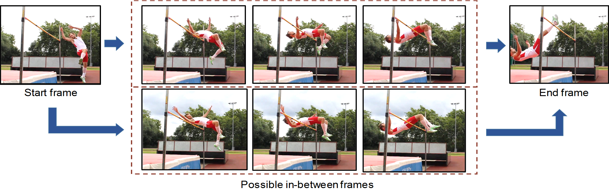
Figure 1: Task of video interpolation. Given a start frame and end frame, humans can speculate or imagine several possible in-between frames. Here shows two possible ways how the high jumper gets over the bar.

In this paper, we aim to tackle the more difficult task of long-term video interpolation, where the missing frames can not receive enough “hints” from nearby frames. We borrow the idea from the predictive models and formulate the process of interpolation as one of bidirectional prediction. Given two non-consecutive frames, we train a convolutional encoder-decoder network to regress to the missing intermediate frames from two opposite directions. We refer to our model as bidirectional predictive network (BiPN), as it consists of a bidirectional encoder-decoder that predicts the future forward from start frame and “predicts” the past backward from end frame at the same time. The bidirectional architecture comes from two critical considerations: (1) Intermediate frames generation requires understanding appearance and motion signals from both start frame and end frame to learn scene transform with time. (2) High-quality long-term predictions are still difficult to achieve since the noise amplifies quickly through time and the prediction degrades dramatically as argued in [8]. Predicting in two direction is a reasonable idea to synthesize roughly double decent intermediate frames.

Our model can understand the input frames and produce a plausible hypothesis for the missing intermediate frames. However, there may exist multiple ways to recover the missing frames as humans can usually imagine multiple paths to get to the final state. As we can see in Fig. 1, a high jumper may get over the bar in different poses. Therefore, this task is inherently multi-modal and much difficult. We make attempts to tackle this multi-modal problem by extending the BiPN with noise vector input. See Section II.C for details.

To produce such frames with more accurate appearance and realistic looking, we combine a loss in image space and feature space with an adversarial loss [9] to train our network. Similar efforts have demonstrated effectivity for generative models such as inpainting [10] and new frames synthesis [8].

The main contributions of this paper are summarized as follows. First, we propose a deep bidirectional predictive network (BiPN) for the challenging task of long-term video interpolation. Second, we extend the BiPN to deal with the multi-modal problem aiming to mimic the diversity of human imagination. Finally, we evaluate our model on a synthetic dataset Moving 2D Shapes and a natural video dataset UCF101 and report competitive results compared to recent approaches both in quantity and quality.

II Approach

We now introduce BiPN, a convolutional encoder-decoder that can predict long-term intermediate frames from two non-consecutive frames. We first present the general architecture and a multi-scale version of BiPN for single procedure generation, then extend the model to tackle the multi-model issue and finally describe the details of training and implementation.

II-A Bidirectional Predictive Network (BiPN)

The general architecture of our BiPN is an encoder-decoder pipeline, including a bidirectional encoder and a single decoder. The bidirectional encoder encodes information from both start frame and end frame and produces a latent feature representation. The decoder takes this feature representation as input to predict multiple missing frames between the two given frames. Fig. 2(b) shows an overview of our architecture.

Bidirectional Encoder. Intuitively, it is inappropriate to predict in-between sequences only utilizing the start frame or the end frame. Instead, predicting multiple intermediate frames requires to understand the appearance and motion signals from both the start and end frames. To this end, we design our encoder as a bidirectional structure, including a forward encoder and a reverse encoder. The forward encoder takes the start frame $f_{st}$ as input and extracts an abstract feature representation $z_{f}$ while the reverse encoder produces representation $z_{r}$ from the end frame $f_{ed}$. Notably, the channels of the end frame are reversed before fed into the reverse encoder. The forward and reverse encoders have the same network architecture, both consisting of several convolutional layers, each with a rectified linear unit (ReLU) followed. The $z_{f}$ and $z_{r}$ are then concatenated into one latent representation $z$.

Decoder. The second half of our pipeline is a single decoder, which processes the latent feature representation $z$ from the above encoder to generate pixels of the in-between frames. The decoder is composed of a series of up-convolutional layers [11] and ReLUs. Finally, the decoder outputs a feature map with the size of $l\times h\times w\times c$ as the prediction of the target in-between frames, where $l$ is the length of frames to be predicted, $h$, $w$ and $c$ are the height, width and the number of channels respectively for each frame ($c=3$ for RGB images).

The BiPN has the advantage to learn temporal dependencies from both start frame and end frame. The bidirectional architecture also comes from another critical consideration: most generative CNNs can only produce decent first few predictions and then the prediction degrades dramatically. Predicting from the start frame and the end frame bidirectionally can synthesize roughly double high quality in-between frames.

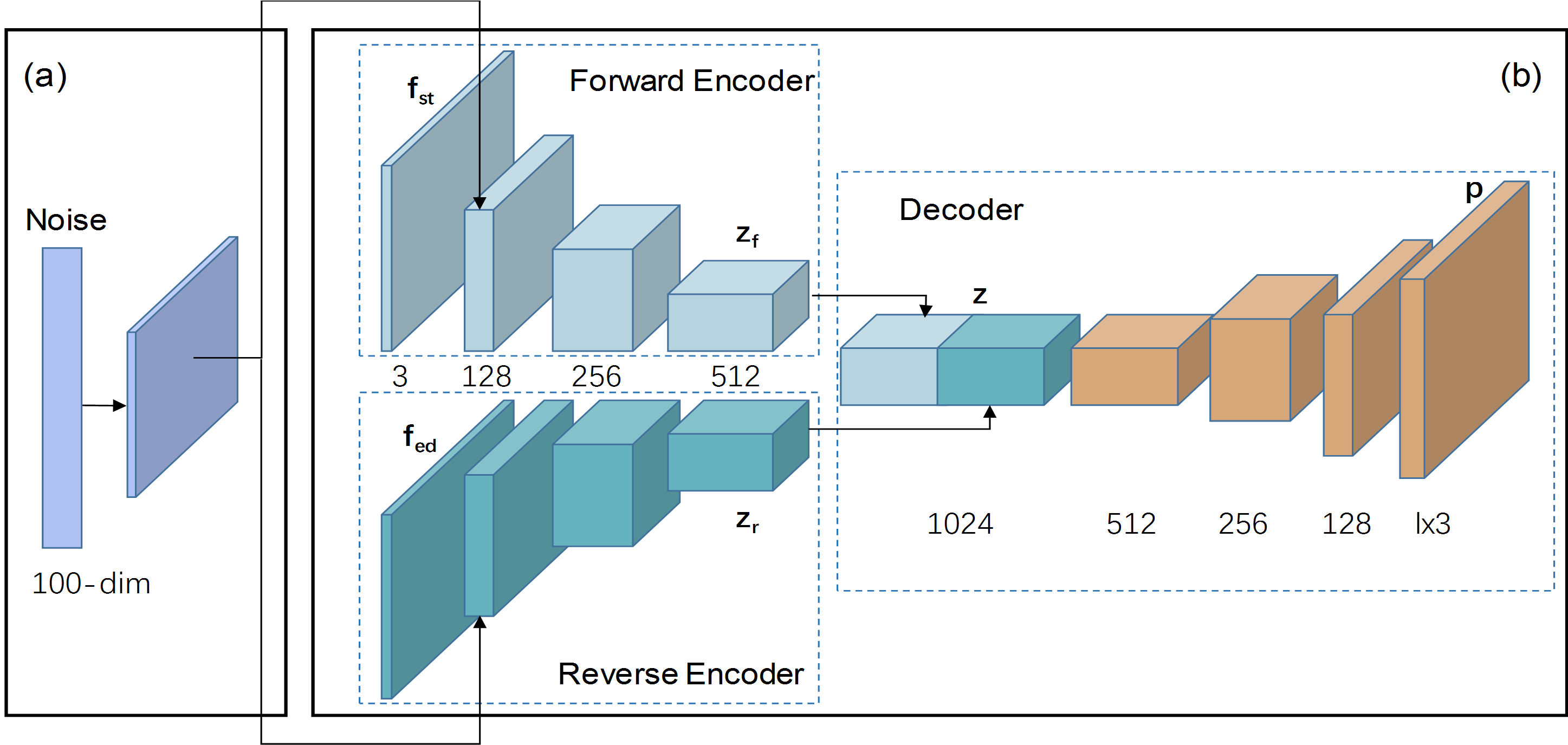
Figure 2: Bidirectional Predictive Network (BiPN). (a) Extended noise input to the network to produce multiple possible intermediate procedures. (b) General architecture of BiPN. The given started frame $f_{st}$ and end frame $f_{ed}$ are passed through the forward encoder and reverse encoder respectively to obtain features $z_{f}$ and $z_{r}$, which are connected to the decoder after concatenated. The decoder finally predicts $l$ in-between frames $p$.

II-B Multi-scale Architecture

Limited by the size of the kernels, convolutions only account for short-range dependencies. This limitation bring difficulties for generative CNNs to encode both large and small motions in a given scene. To tackle this problem, we enrich our BiPN into a multi-scale architecture, which has been adopted in many prediction works [6] [5] and proved to be effective.

We employ $4$ scales ($k=1,2,3,4$) and design $4$ BiPNs in practice. The multi-scale architecture is shown in Fig. 3. Given an origin frame of size $s\times s$ for scale $k=4$, denoted as $x_{4}$, the frame is resized to $\frac{1}{2}s\times\frac{1}{2}s$, $\frac{1}{4}s\times\frac{1}{4}s$ and $\frac{1}{8}s\times\frac{1}{8}s$ images (defined as $x_{3},x_{2},x_{1}$) for $k=3,2,1$ respectively. These images of different sizes are fed into different BiPNs to produce multiple scales of in-between frames $p_{k}$. It is worth noting that these BiPNs do not process images $x_{1,2,3,4}$ in a parallel but a sequential way. In more details, the first prediction $p_{1}$ produced by $\textnormal{BiPN}_{1}$ is upsampled to $\frac{1}{4}s\times\frac{1}{4}s$ and then concatenated to $x_{2}$ as input of $\textnormal{BiPN}_{2}$. In the same way, $p_{2}$ and $p_{3}$ are used as auxiliary inputs to $\textnormal{BiPN}_{3}$ and $\textnormal{BiPN}_{4}$. The output $p_{4}$ of $\textnormal{BiPN}_{4}$ is chosen as the final prediction.

II-C Multi-modal Procedures

Given an initial state and a final state, the BiPN presented above can only predict one possible procedure for a specific scene. However, in most cases, people tend to imagine multiple potential pathways or situations to get to the target state as shown in Fig. 1. To mimic this human behavior, we extend our BiPN to explore the space of possible actions by adding a random Gaussian noise to the encoder. Passing the start and end frames as input and sampling from the noise variable allow the model to predict multiple possible sets of in-between frames according to multiple different input noises. The extended part of the architecture is shown in Fig. 2. To the best of our knowledge, we are the first to address the multi-modal problem in long-term video interpolation.

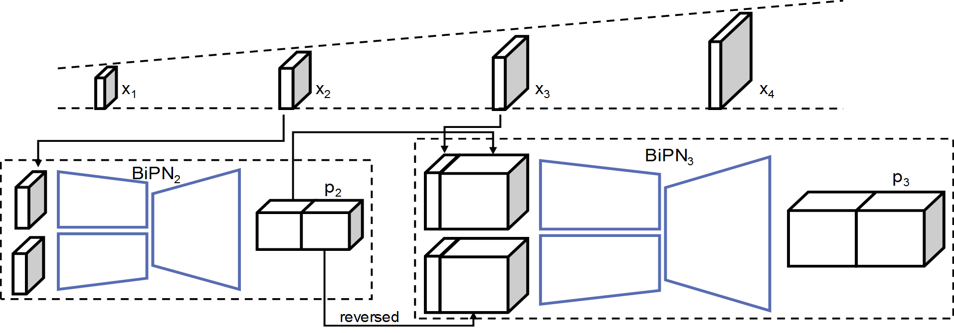
Figure 3: Multi-scale BiPN. Intermediate frames are obtained from a coarse to fine scale. Prediction from lower resolutions are split into two halves and next concatenated to start frame and end frame at higher resolutions as auxiliary inputs. We only show the details of scale $2$ and $3$ here.

II-D Training

We train BiPN by regressing to the ground truth in-between frames. We clip each video into small sequences to construct training and test sets. Given a training sequence $X=\{x_{1},x_{2},...,x_{T}\}$, we use $x_{1}$ and $x_{T}$ as start frame and end frame. The remaining frames are used as ground truth.

To synthesize high-quality and realistic frames, we optimize our network to minimize distance between the predicted frames and target frames in both image space and feature space, as well as minimize the adversarial loss [9]. Thus the joint loss function of our network can be defined as:

$$L=L_{rec}+L_{feat}+L_{adv},$$ (1)

where $L_{rec}$ is the $L_{2}$ reconstruction loss responsible for producing a rough outline of the predicted frames. However, $L_{2}$ loss often results in blurry averaged images. $L_{feat}$ is the loss in feature space aiming to predict frames with more accurate appearance. We use the feature maps from the last convolutional layer of AlexNet [12]. $L_{adv}$ is the adversarial loss, which is introduced by GAN [9] and has been adopted by many recent generative models to produce realistic images. Since our BiPN produces a small video sequence instead of a single image each time, we need to design a discriminator $D$ that tries to distinguish real and fake videos. We utilize multiple spatio-temporal convolutional layers to construct $D$. The $L_{rec}$, $L_{feat}$ and $L_{adv}$ can be expressed as following:

$$L_{rec}=\sum\nolimits_{k=1}^{N_{scales}}\left\|p_{k}-\hat{p_{k}}\right\|_{2}^{2},$$ (2)

$$L_{feat}=\sum\nolimits_{k=1}^{N_{scales}}\left\|Alex(p_{k})-Alex(\hat{p_{k}})\right\|_{2}^{2},$$ (3)

$$L_{adv}=\sum\nolimits_{k=1}^{N_{scales}}L_{bce}(D_{k}(\hat{p_{k}}),1)$$ (4)

where $p_{k}$ and $\hat{p_{k}}$ are ground truth frames and our prediction respectively at scale $k$. $Alex(\cdot)$ indicates extracted features from all images in the sequence using AlexNet. $L_{bce}$ is the binary cross-entropy loss. During the multi-modal training, $L_{rec}$ is not used since it will restrict the diversity of outputs.

II-E Implementation Details

Our model is implemented using TensorFlow and deployed on the Tesla K80 GPU. For a multi-scale deterministic BiPN model, both forward encoder and reverse encoder consist of $3$ convolutional layers while the decoder contains $4$ up-convolutional layers. The sizes of convolution kernels are diverse at different depths and scales. For multi-scale non-deterministic BiPN model, the basic architecture is almost the same with the deterministic one but adding an additional 100-dimensional noise vector as input. The noise is first passed through a fully-connected layer, reshaped to a feature map, and then concatenated to the intermediate feature map of the forward and reverse encoders. All input frames are resized to $64\times 64$ in training while kept the original sizes during testing.

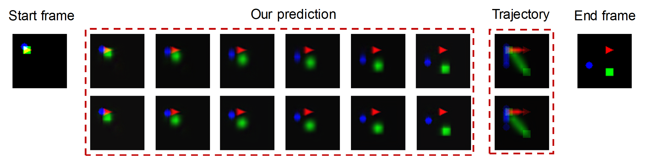
Figure 4: Two different sets of possible in-between frames are predicted by sampling different noise. Differences can be seen from two trajectory images.

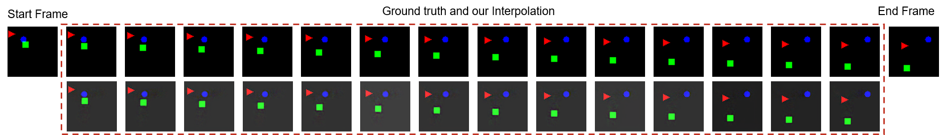
Figure 5: 2D Shape results of interpolating $14$ frames. All objects of our interpolation in second row can move to the right positions as well as keep their original appearance unchanged compared to the ground truth in the first row.

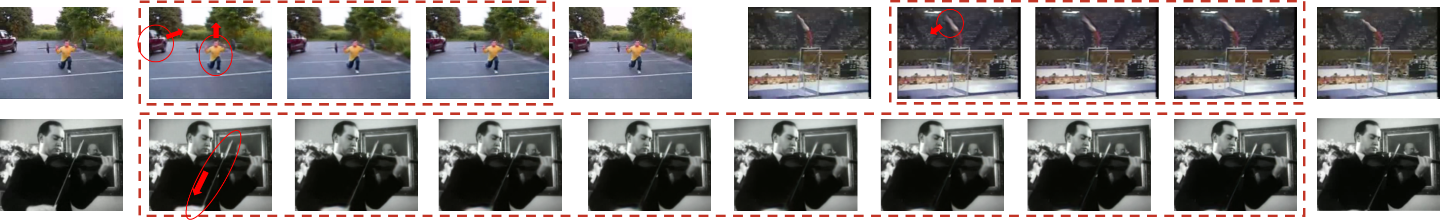
Figure 6: UCF101 results. First row: $2$ examples of interpolating $3$ frames. Notice the movements of the car, the weightlifter (ex$1$.) and the feet of the gymnast (ex$2$.). Second row: $1$ example of interpolating 8 frames that details how the violinist plays the violin. The red arrows indicate the moving directions.

III Experiments

In this section, we evaluate our model on two datasets. We first conduct experiments using the dataset of synthetic 2D shapes to perform qualitative analysis. We then experiment our model for natural high-resolution videos using the UCF101 dataset and compare the results to recent outstanding methods.

III-A Moving 2D Shapes

Moving 2D Shapes is a synthetic dataset containing three types of objects moving inside $64\times 64$ frames, where circles, squares and triangles move in random direction (vertically, horizontally or diagonally) with random velocity. Fig. 5 shows our qualitative results with $14$ frames generated from only $2$ input frames. We can see that our interpolation results are quite close to the ground truth. In addition, as can be seen in Fig. 4, adding different noise samples to the non-deterministic model can produce multiple plausible motions as expected.

Experiments on this toy dataset demonstrate that our BiPN model can predict long-term in-between frames, capture the trajectories of different objects accurately and has the ability to produce multiple possible intermediate procedures.

III-B UCF101 Dataset

The UCF101 dataset [13] contains $13,320$ videos belonging to $101$ action categories and each video has a resolution of $240\times 320$. We sample $200,000$ video sequences from the training set to train BiPN and use the same test set with [6] [5] as benchmarks. Both Peak Signal to Noise Ratio (PSNR) and Structural Similarity Index Measure (SSIM) [14] are used to assess the image quality of the predicted frames, where higher PSNR and SSIM are better.

Fig. 7 shows the change of generator loss and SharpDiff of the single-scale and multi-scale BiPN with different training iterations. We can see that the multi-scale BiPN obtains lower loss and higher SharpDiff than the single one. We further compare our approach against several outstanding methods, including the optical flow technique EpicFlow [3] and DVF [5]. To be comparable, we evaluate BiPN on single-frame generation as the published results of EpicFlow and DVF are obtained by only evaluating one in-between frame. The results are reported in Table I, which shows that multi-scale BiPN brings moderate improvement to the single-scale one. Also, our model can achieve better PSNR than EpicFlow and DVF as well as competitive performance in terms of SSIM.

Speculating the long-term procedures of events and further synthesizing frames in natural videos are rather difficult. Our BiPN can generate more than $8$ decent frames as shown in Fig. 6. More results can be found in our supplementary material.

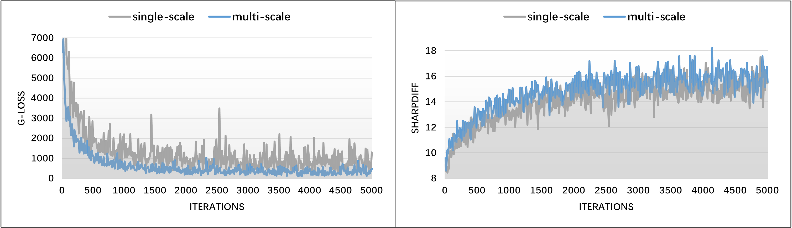
Figure 7: Generator loss and SharpDiff [6] (a measure for sharpness, higher is better) comparison of single-scale and multi-scale BiPN on UCF101 dataset.

IV Conclusion

This paper introduces a bidirectional predictive network (BiPN) for long-term video interpolation. BiPN is built as an encoder-decoder model that can predict the intermediate frames in two opposite direction. A multi-scale version of BiPN is also developed to capture both small and large motions. To enable the model to imagine multiple possible motions, we feed the BiPN with an extra noise vector input as exploratory experiment. We demonstrate the advantages of BiPN on Moving 2D Shapes and UCF101 dataset and report competitive results to the recent approaches.

TABLE I: PSNR and SSIM comparison on UCF101.

Model	PSNR	SSIM
EpicFlow [3]	30.2	0.93
DVF [5]	30.9	0.94
Single-scale BiPN (ours)	30.6	0.92
Multi-scale BiPN (ours)	31.4	0.94

References

- [1] S. Baker, D. Scharstein, J. Lewis, S. Roth, M. J. Black, and R. Szeliski, “A database and evaluation methodology for optical flow,” IJCV, vol. 92, no. 1, pp. 1–31, 2011.
- [2] C. Zhang and T. Chen, “A survey on image-based rendering representation, sampling and compression,” Signal Processing: Image Communication, vol. 19, no. 1, pp. 1–28, 2004.
- [3] J. Revaud, P. Weinzaepfel, Z. Harchaoui, and C. Schmid, “Epicflow: Edge-preserving interpolation of correspondences for optical flow,” in CVPR, 2015, pp. 1164–1172.
- [4] S. Niklaus, L. Mai, and F. Liu, “Video frame interpolation via adaptive convolution,” arXiv preprint arXiv:1703.07514, 2017.
- [5] Z. Liu, R. Yeh, X. Tang, Y. Liu, and A. Agarwala, “Video frame synthesis using deep voxel flow,” arXiv preprint arXiv:1702.02463, 2017.
- [6] M. Mathieu, C. Couprie, and Y. LeCun, “Deep multi-scale video prediction beyond mean square error,” arXiv preprint arXiv:1511.05440, 2015.
- [7] C. Vondrick, H. Pirsiavash, and A. Torralba, “Generating videos with scene dynamics,” in NIPS, 2016, pp. 613–621.
- [8] R. Villegas, J. Yang, Y. Zou, S. Sohn, X. Lin, and H. Lee, “Learning to generate long-term future via hierarchical prediction,” arXiv preprint arXiv:1704.05831, 2017.
- [9] I. Goodfellow, J. Pouget-Abadie, M. Mirza, B. Xu, D. Warde-Farley, S. Ozair, A. Courville, and Y. Bengio, “Generative adversarial nets,” in NIPS, 2014, pp. 2672–2680.
- [10] D. Pathak, P. Krahenbuhl, J. Donahue, T. Darrell, and A. A. Efros, “Context encoders: Feature learning by inpainting,” in CVPR, 2016, pp. 2536–2544.
- [11] A. Dosovitskiy, J. Tobias Springenberg, and T. Brox, “Learning to generate chairs with convolutional neural networks,” in CVPR, 2015, pp. 1538–1546.
- [12] A. Krizhevsky, I. Sutskever, and G. E. Hinton, “Imagenet classification with deep convolutional neural networks,” in NIPS, 2012, pp. 1097–1105.
- [13] K. Soomro, A. R. Zamir, and M. Shah, “Ucf101: A dataset of 101 human actions classes from videos in the wild,” arXiv preprint arXiv:1212.0402, 2012.
- [14] Z. Wang, A. C. Bovik, H. R. Sheikh, and E. P. Simoncelli, “Image quality assessment: from error visibility to structural similarity,” IEEE transactions on image processing, vol. 13, no. 4, pp. 600–612, 2004.