Analyzing the Robustness of Nearest Neighbors to Adversarial Examples
Abstract
Motivated by safety-critical applications, test-time attacks on classifiers via adversarial examples has recently received a great deal of attention. However, there is a general lack of understanding on why adversarial examples arise; whether they originate due to inherent properties of data or due to lack of training samples remains ill-understood. In this work, we introduce a theoretical framework analogous to bias-variance theory for understanding these effects. We use our framework to analyze the robustness of a canonical non-parametric classifier – the -nearest neighbors. Our analysis shows that its robustness properties depend critically on the value of – the classifier may be inherently non-robust for small k, but its robustness approaches that of the Bayes Optimal classifier for fast-growing . We propose a novel modified -nearest neighbor classifier, and guarantee its robustness in the large sample limit. Our experiments 111Code available at: https://github.com/EricYizhenWang/robust_nn_icml suggest that this classifier may have good robustness properties even for reasonable data set sizes.
1 Introduction
Machine learning is increasingly applied in security-critical domains such as automotive systems, healthcare, finance and robotics. To ensure safe deployment in these applications, there is an increasing need to design machine-learning algorithms that are robust in the presence of adversarial attacks.
A realistic attack paradigm that has received a lot of recent attention [12, 26, 28, 25] is test-time attacks via adversarial examples. Here, an adversary has the ability to provide modified test inputs to an already-trained classifier, but cannot modify the training process in any way. Their goal is to perturb legitimate test inputs by a “small amount” in order to force the classifier to report an incorrect label. An example is an adversary that replaces a stop sign by a slightly defaced version in order to force an autonomous vehicle to recognize it as an yield sign. This attack is undetectable to the human eye if the perturbation is small enough.
Prior work has considered adversarial examples in the context of linear classifiers [19], kernel SVMs [3] and neural networks [28, 12, 25, 26, 22]. However, most of this work has either been empirical, or has focussed on developing theoretically motivated attacks and defenses. Consequently, there is a general lack of understanding on why adversarial examples arise; whether they originate due to inherent properties of data or due to lack of training samples remains ill-understood.
This work develops a theoretical framework for robust learning in order to understand the effects of distributional properties and finite samples on robustness. Building on traditional bias-variance theory [10], we posit that a classification algorithm may be robust to adversarial examples due to three reasons. First, it may be distributionally robust, in the sense that the output classifier is robust as the number of training samples grow to infinity. Second, even the output of a distributionally robust classification algorithm may be vulnerable due to too few training samples – this is characterized by finite sample robustness. Finally, different training algorithms might result in classifiers with different degrees of robustness, which we call algorithmic robustness. These quantities are analogous to bias, variance and algorithmic effects respectively.
Next, we analyze a simple non-parametric classification algorithm: -nearest neighbors in our framework. Our analysis demonstrates that large sample robustness properties of this algorithm depend very much on .
Specifically, we identify two distinct regimes for with vastly different robustness properties. When is constant, we show that -nearest neighbors has zero robustness in the large sample limit in regions where lies in . This is in contrast with accuracy, which may be quite high in these regions. For , where is the data dimension and is the sample size, we show that the robustness region of -nearest neighbors approaches that of the Bayes Optimal classifier in the large sample limit. This is again in contrast with accuracy, where convergence to the Bayes Optimal accuracy is known for a much slower growing [7, 5].
Since is too high to use in practice with nearest neighbors, we next propose a novel robust version of the -nearest neighbor classifier that operates on a modified training set. We provably show that in the large sample limit, this algorithm has superior robustness to standard -nearest neighbors for data distributions with certain properties.
Finally, we validate our theoretical results by empirically evaluating our algorithm on three datasets against several popular attacks. Our experiments demonstrate that our algorithm performs better than or about as well as both standard -nearest neighbors and nearest neighbors with adversarial training – a popular and effective defense mechanism. This suggests that although our performance guarantees hold in the large sample limit, our algorithm may have good robustness properties even for realistic training data sizes.
1.1 Related Work
Adversarial examples have recently received a great deal of attention [12, 3, 26, 28, 25]. Most of the work, however, has been empirical, and has focussed on developing increasingly sophisticated attacks and defenses.
1.1.1 Related Work on Adversarial Examples
Prior theoretical work on adversarial examples falls into two categories – analysis and theory-inspired defenses. Work on analysis includes [9], which analyzes the robustness of linear and quadratic classifiers under random and semi-random perturbations. [13] provides robustness guarantees on linear and kernel classifiers trained on a given data set. [11] shows that linear classifiers for high dimensional datasets may have inherent robustness-accuracy trade-offs.
Work on theory-inspired defenses include [20, 15, 1], who provide defense mechanisms for adversarial examples in neural networks that are relaxations of certain principled optimization objectives. [14] shows how to use program verification to certify robustness of neural networks around given inputs for small neural networks.
Our work differs from these in two important ways. First, unlike most prior work which looks at a given training dataset, we consider effects of the data distribution and number of samples, and analyze robustness properties in the large sample limit. Second, unlike prior work which largely focuses on parametric methods such as neural networks, our focus is on a canonical non-parametric method – the nearest neighbors classifier.
1.1.2 Related Work on Nearest Neighbors
There has been a body of work on the convergence and consistency of nearest-neighbor classifiers and their many variants [6, 27, 17, 8, 5, 16]; all these works however consider accuracy and not robustness.
In the asymptotic regime, [6] shows that the accuracy of -nearest neighbors converges in the large sample limit to where is the error rate of the Bayes Optimal classifier. This implies that even -nearest neighbor may achieve relatively high accuracy even when is not or . In contrast, we show that -nearest neighbor is inherently non-robust when under some continuity conditions.
For larger , the accuracy of -nearest neighbors is known to converge to that of the Bayes Optimal classifier if and as the sample size . We show that the robustness also converges to that of the Bayes Optimal classifier when grows at a much higher rate – fast enough to ensure uniform convergence. Whether this high rate is necessary remains an intriguing open question.
Finite sample rates on the accuracy of nearest neighbors are known to depend heavily on properties of the data distribution, and there is no distribution free rate as in parametric methods [8]. [5] provides a clean characterization of the finite sample rates of nearest neighbors as a function of natural interiors of the classes. Here we build on their results by defining a stricter, more robust version of interiors and providing bounds as functions of these new robust quantities.
1.1.3 Other Related Work
[2] provides a method for generating adversarial examples for nearest neighbors, and shows that the effectiveness of attacks grow with intrinsic dimensionality. Finally, [24, 25] provides black-box attacks on substitute classifiers; their experiments show that attacks from other types of substitute classifiers are not successful on nearest neighbors; our experiments corroborate these results.
2 The Setting and Definitions
2.1 The Basic Setup
We consider test-time attacks in a white box setting, where the adversary has full knowledge of the training process – namely, the type of classifier used, the training data and any parameters – but cannot modify training in any way.
Given an input , the adversary’s goal is to perturb it so as to force the trained classifier to report a different label than . The amount of perturbation is measured by an application-specific metric , and is constrained to be within a radius . Our analysis can be extended to any metric, but for this paper we assume that is the Euclidean distance for mathematical simplicity; we also focus on binary classification, and leave extensions to multiclass for future work.
Finally, we assume that unlabeled instances are drawn from an instance space , and their labels are drawn from the label space . There is an underlying data distribution that generates labeled examples; the marginal over of is and the conditional distribution of labels given is denoted by .
2.2 Robustness and astuteness
We begin by defining robustness, which for a classifier at input is measured by the robustness radius.
Definition 2.1 (Robustness Radius).
The robustness radius of a classifier at an instance , denoted by , is the shortest distance between and an input to which assigns a label different from :
Observe that the robustness radius measures a classifier’s local robustness. A classifier with robustness radius at guarantees that no adversarial example of with norm of perturbation less than can be created using any attack method. A plausible way to extend this into a global notion is to require a lower bound on the robustness radius everywhere; however, only the constant classifier will satisfy this condition. Instead, we consider robustness around meaningful instances, that we model as examples drawn from the underlying data distribution.
Definition 2.2 (Robustness with respect to a Distribution).
The robustness of a classifier at radius with respect to a distribution over the instance space , denoted by , is the fraction of instances drawn from for which the robustness radius is greater than or equal to .
Finally, observe that we are interested in classifiers that are both robust and accurate. This leads to the notion of astuteness, which measures the fraction of instances on which a classifier is both accurate and robust.
Definition 2.3 (astuteness).
The astuteness of a classifier with respect to a data distribution and a radius is the fraction of examples on which it is accurate and has robustness radius at least ; formally,
Observe that astuteness is analogous to classification accuracy, and we argue that it is a more appropriate metric if we are concerned with both robustness and accuracy. Unlike accuracy, astuteness cannot be directly empirically measured unless we have a way to certify a lower bound on the robustness radius. In this work, we will prove bounds on the astuteness of classifiers, and in our experiments, we will approximate it by measuring resistance to standard attacks.
2.3 Sources of Robustness
There are three plausible reasons why classifiers lack robustness – distributional, finite sample and algorithmic. These sources are analogous to bias, variance, and algorithmic effects respectively in standard bias-variance theory.
Distributional robustness measures the effect of the data distribution on robustness when an infinitely large number of samples are used to train the classifier. Formally, if is a training sample of size drawn from and is a classifier obtained by applying the training procedure on , then the distributional robustness at radius is .
In contrast, for finite sample robustness, we characterize the behaviour of for finite – usually by putting high probability bounds over the training set. Thus, finite sample robustness depends on the training set size , and quantifies how it changes with sample size. Finally, robustness also depends on the training algorithm itself; for example, some variants of nearest neighbors may have higher robustness than nearest neighbors itself.
2.4 Nearest Neighbor and Bayes Optimal Classifiers
Given a training set and a test example , we use the notation to denote the -th nearest neighbor of in , and to denote the label of .
Given a test example , the -nearest neighbor classifier outputs:
| otherwise. |
The Bayes optimal classifier over a data distribution has the following classification rule:
| (1) |
3 Robustness of Nearest Neighbors
How robust is the -nearest neighbor classifier? We show that it depends on the value of . Specifically, we identify two distinct regimes – constant and where is the data dimension – and show that nearest neighbors has different robustness properties in the two.
3.1 Low Regime
In this region, is a constant that does not depend on the training set size . Provided certain regularity conditions hold, we show that -nearest neighbors is inherently non-robust in this regime unless – in the sense that the distributional robustness becomes in the large sample limit.
Theorem 3.1.
Let such that (a) is absolutely continuous with respect to the Lebesgue measure (b) (c) is continuous with respect to the Euclidean metric in a neighborhood of . Then, for fixed , converges in probability to .
Remarks.
Observe that Theorem 3.1 implies that the distributional robustness (and hence astuteness) in a region where is . This is in contrast with accuracy; for -NN, the accuracy converges to as , where is the error rate of the Bayes Optimal classifier, and thus may be quite high.
The proof of Theorem 3.1 in the Appendix shows that the absolute continuity of with respect to the Lebesgue measure is not strictly necessary; absolute continuity with respect to an embedded manifold will give the same result, but will result in a more complex proof.
In the Appendix A (Theorem A.2), we show that -nearest neighbor is astute in the interior of the region where , and provide finite sample rates for this case.
3.2 High Regime
Prior work has shown that in the large sample limit, the accuracy of the nearest neighbor classifiers converge to the Bayes Optimal, provided is set properly. We next show that if is , the regions of robustness and the astuteness of the nearest neighbor classifiers also approach the corresponding quantities for the Bayes Optimal classifier as . Thus, if the Bayes Optimal classifier is robust, then so is -nearest neighbors in the large sample limit.
The main intuition is that is large enough for uniform convergence – where, with high probability, all Euclidean balls with examples have the property that the empirical averages of their labels are close to their expectations. This guarantees that for any , the -nearest neighbor reports the same label as the Bayes Optimal classifier for all close to . Thus, if the Bayes Optimal classifier is robust, so is nearest neighbors.
3.2.1 Definitions
We begin with some definitions that we can use to characterize the robustness of the Bayes Optimal classifier. Following [5], we use the notation to denote an open ball and to denote a closed ball of radius around . We define the probability radius of a ball around as:
We next define the -robust -strict interiors as follows:
What is the significance of these interiors? Let be an instance such that all have . If , then the points closest to have . Provided the average of the labels of these points is close to expectation, which happens when is large relative to , -nearest neighbor outputs label on . When is in the -robust -strict interior region , this is true for all within distance of , which means that -nearest neighbors will be robust at . Thus, the -robust -strict interior is the region where we natually expect -nearest neighbor to have robustness radius , when is large relative to and .
Readers familiar with [5] will observe that the set of all for which forms a stricter version of the -interiors of the region that was defined in this work; these also represent the region where -nearest neighbors are accurate when . The -robust -strict interior is thus a somewhat stricter and more robust version of this definition.
3.2.2 Main Results
We begin by characterizing where the Bayes Optimal classifier is robust.
Theorem 3.2.
The Bayes Optimal classifier has robustness radius at . Moreover, its astuteness is .
The proof is in the Appendix, along with analogous results for astuteness. The following theorem, along with a similar result for astuteness, proved in the Appendix, characterizes robustness in the large regime.
Theorem 3.3.
For any , pick a and a . There exist constant and such that if , and , then, with probability , -NN has robustness radius in .
Remarks.
Some remarks are in order. First, observe that as , and tend to ; thus, provided certain continuity conditions hold, approaches , the robustness region of the Bayes Optimal classifier.
4 A Robust 1-NN Algorithm
Section 3 shows that nearest neighbors is robust for as large as . However, this is too high to use in practice – high values of require even higher sample sizes [5], and lead to higher running times. Thus a natural question is whether we can find a more robust version of the algorithm for smaller . In this section, we provide a more robust version of -nearest neighbors, and analytically demonstrate its robustness.
Our algorithm is motivated by the observation that -nearest neighbor is robust when oppositely labeled points are far apart, and when test points lie close to training data. Most training datasets however contain nearby points that are oppositely labeled; thus, we propose to remove a subset of training points to enforce this property.
Which points should we remove? A plausible approach is to keep the largest subset where oppositely labeled points are far apart; however, this subset has poor stability properties even for large . Therefore, we propose to keep all points such that: (a) we are highly confident about the label of and its nearby points and (b) all points close to have the same label. Given that all such are kept, we remove as few points as possible, and execute nearest neighbors on the remaining dataset.
The following definition characterizes data where oppositely labeled points are far apart.
Definition 4.1 (-separated set).
A set of labeled examples is said to be -separated if for all pairs , implies .
The full algorithm is described in Algorithm 1 and Algorithm 2. Given confidence parameters and , Algorithm 2 returns a label when this label agrees with the average of points closest to ; otherwise, it returns . is chosen such that with probability , the empirical majority of labels agrees with the majority in expectation, provided the latter is at least away from .
Algorithm 2 is used to determine whether an should be kept. Let be the output of Algorithm 2 on . If and if for all , , then we mark as red. Finally, we compute the largest -separated subset of the training data that includes all the red points; this reduces to a constrained matching problem as in [16]. The resulting set, returned by Algorithm 1, is our new training set. We observe that this set is -separated from Lemma B.2 in the Appendix, and thus oppositely labeled points are far apart. Moreover, we keep all when we are confident about the label of and its nearby points. Observe that our final procedure is a 1-NN algorithm, even though neighbors are used to determine if a point should be retained in the training set.
4.1 Performance Guarantees
The following theorem establishes performance guarantees for Algorithm 1.
Theorem 4.2.
Pick a and , and set . Pick a margin parameter . Then, there exist constants and such that the following hold. If we set , and define the set:
Then, with probability over the training set, Algorithm 1 run with parameters , and has robustness radius at least on .
Remarks.
The proof is in the Appendix, along with an analogous result for astuteness. Observe that is roughly the high density subset of the -robust strict interior . Since is constrained to be greater than or less than in this region, as opposed to or , this is an improvement over standard nearest neighbors when the data distribution has a large high density region that intersects with the interiors.
A second observation is that as is an arbitrary constant, we can set to it be quite small and still satisfy the condition on for a large fraction of ’s when is very large. This means that in the large sample limit, may be close to and may be close to the high density subset of for a lot of smooth distributions.
5 Experiments
The results in Section 4 assume large sample limits. Thus, a natural question is how well Algorithm 1 performs with more reasonable amounts of training data. We now empirically investigate this question.
Since there are no general methods that certify robustness at an input, we assess robustness by measuring how our algorithm performs against a suite of standard attack methods. Specifically, we consider the following questions:
-
1.
1. How does our algorithm perform against popular white box and black box attacks compared with standard baselines?
-
2.
2. How is performance affected when we change the training set size relative to the data dimension?
These questions are considered in the context of three datasets with varying training set sizes relative to the dimension, as well as two standard white box attacks and black box attacks with two kinds of substitute classifiers.
5.1 Methodology
5.1.1 Data
We use three datasets – Halfmoon, MNIST 1v7 and Abalone – with differing data sizes relative to dimension. Halfmoon is a popular -dimensional synthetic data set for non-linear classification. We use a training set of size and a test set of size generated with standard deviation . The MNIST 1v7 data set is a subset of the -dimensional MNIST data. For training, we use images each of Digit 1 and 7, and for test, images of each digit. Finally, for the Abalone dataset [18], our classification task is to distinguish whether an abalone is older than 12.5 years based on physical measurements. For training, we use and for test, samples. In addition, a validation set with the same size as the test set is generated for each experiment for parameter tuning.
5.1.2 Baselines
We compare Algorithm 1, denoted by RobustNN, against three baselines. The first is the standard -nearest neighbor algorithm, denoted by StandardNN. We use two forms of adversarially-trained nearest neighbors - ATNN and ATNN-all. Let be the training set used by standard nearest neighbors. In ATNN, we augment by creating, for each , an adversarial example using the attack method in the experiment, and adding . The ATNN classifier is -nearest neighbor on this augmented data. In ATNN-all, for each , we create adversarial examples using all the attack methods in the experiment, and add them all to . ATNN-all is the nearest neighbor classifier on this augmented data. For example, for white box Direct Attacks in Section 5.2, ATNN includes adversarial examples generated by the Direct Attack, and ATNN-all includes adversarial examples generated by both Direct and Kernel Substitute Attacks.
Observe that all algorithms except StandardNN have parameters to tune. RobustNN has three input parameters – and a defense radius which is an approximation to the robustness radius. For simplicity, we set , and tune on the validation set; this can be viewed as tuning the parameter in Theorem 4.2. For ATNN and ATNN-all, the methods that generate the augmenting adversarial examples need a perturbation magnitude ; we call this the defense radius. To be fair to all algorithms, we tune the defense radius for each. We consider the adversary with the highest attack perturbation magnitude in the experiment, and select the defense radius that yields the highest validation accuracy against this adversary.
5.2 White-box Attacks and Results
To evaluate the robustness of Algorithm 1, we use two standard classes of attacks – white box and black box. For white-box attacks, the adversary knows all details about the classifier under attack, including its training data, the training algorithm and any hyperparameters.
5.2.1 Attack Methods
Direct Attack. This attack takes as input a test example , an attack radius , and a training dataset (which may be an augmented or reduced dataset). It finds an that is closest to but has a different label, and returns the adversarial example .
Kernel Substitute Attack. This method attacks a substitute kernel classifier trained on the same training set. For a test input , a set of training points with one-hot labels , a kernel classifier predicts the class probability as:
The adversary trains a kernel classifier on the training set of the corresponding nearest neighbors, and then generates adversarial examples against this kernel classifier. The advantage is that the prediction of the kernel classifier is differentiable, which allows the use of standard gradient-based attack methods. For our experiments, we use the popular fast-gradient-sign method (FSGM). The parameter is tuned to yield the most effective attack, and is set to for Halfmoon and MNIST, and for Abalone.
5.2.2 Results
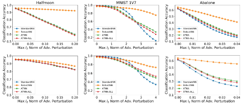
Figure 1 shows the results. We see that RobustNN outperforms all baselines for Halfmoon and Abalone for all attack radii. For MNIST, for low attack radii, RobustNN’s classification accuracy is slightly lower than the others, while it outperforms the others for large attack radii. Additionally, as is to be expected, the Direct Attack results in lower general accuracy than the Kernel Substitute Attack.
These results suggest that our algorithm mostly outperforms the baselines StandardNN, ATNN and ATNN-all. As predicted by theory, the performance gain is higher when the training set size is large relative to the dimension – which is the setting where nearest neighbors work well in general. It has superior performance for Halfmoon and Abalone, where the training set size is large to medium relative to dimension. In contrast, in the sparse dataset MNIST, our algorithm has slightly lower classification accuracy for small attack radii, and higher otherwise.
5.3 Black-box Attacks and Results
[25] has observed that some defense methods that work by masking gradients remain highly amenable to black box attacks. In this attack, the adversary is unaware of the target classifier’s nature, parameters or training data, but has access to a seed dataset drawn from the same distribution which they use to train and attack a substitute classifier. To establish robustness properties of Algorithm 1, we therefore validate it against black box attacks based on two types of substitute classifiers.
5.3.1 Attack Methods
We use two types of substitute classifiers – kernel classifiers and neural networks. The adversary trains the substitute classifier using the method of [25] and uses the adversarial examples against the substitute to attack the target classifier.
Kernel Classifier. The kernel classifier substitute is the same as the one in Section 5.2, but trained using the seed data and the method of [25].
Neural Networks. The neural network for MNIST is the ConvNet in [23]’s tutorial. For Halfmoon and Abalone, the network is a multi-layer perceptron with hidden layers.
Procedure. To train the substitute classifier, the adversary uses the method of [24] to augment the seed data for two rounds; labels are obtained by querying the target classifier. Adversarial examples against the substitutes are created by FGSM, following [24]. As a sanity check, we verify the performance of the substitute classifiers on the original training and test sets. Details are in Table 1 in the Appendix. Sanity checks on the performance of the substitute classifiers are presented in Table 1 in the Appendix.
5.3.2 Results
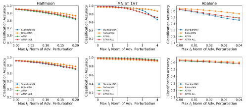
Figure 2 shows the results. For all algorithms, black box attacks are less effective than white box, which corroborates the results of [24], who observed that black-box attacks are less successful against nearest neighbors. We also find that the kernel substitute attack is more effective than the neural network substitute, which is expected as kernel classifiers have similar structure to nearest neighbors. Finally, for Halfmoon and Abalone, our algorithm outperforms the baselines for both attacks; however, for MNIST neural network substitute, our algorithm does not perform as well for small attack radii. This again confirms the theoretical predictions that our algorithm’s performance is better when the training set is large relative to the data dimension – the setting in which nearest neighbors work well in general.
5.4 Discussion
The results show that our algorithm performs either better than or about the same as standard baselines against popular white box and black box attacks. As expected from our theoretical results, it performs better for denser datasets which have high or medium amounts of training data relative to the dimension, and either slightly worse or better for sparser datasets, depending on the attack radius. Since non-parametric methods such as nearest neighbors are mostly used for dense data, this suggests that our algorithm has good robustness properties even with reasonable amounts of training data.
6 Conclusion
We introduce a novel theoretical framework for learning robust to adversarial examples, and introduce notions of distributional and finite-sample robustness. We use these notions to analyze a non-parametric classifier, -nearest neighbors, and introduce a novel modified -nearest neighbor algorithm that has good robustness properties in the large sample limit. Experiments show that these properties are still retained for reasonable data sizes.
Many open questions remain. The first is to close the gap in analysis of -nearest neighbors for in between our two regimes. The second is to develop nearest neighbor algorithms with better robustness guarantees. Finally, we believe that our work is a first step towards a comprehensive analysis of how the size of training data affects robustness; we believe that an important line of future work is to carry out similar analyses for other supervised learning methods.
Acknowledgement
We thank NSF under IIS 1253942 for support. This work was also partially supported by ARO under contract number W911NF-1-0405. We thank all anonymous reviewers for their constructive comments.
We also thank Rabanus Derr from University of Tübingen for pointing about a minor mistake in the proof of Lemma B.3. The proof is fixed in the latest version.
References
- [1] John Duchi Aman Sinha, Hongseok Namkoong. Certifiable distributional robustness with principled adversarial training. International Conference on Learning Representations, 2018.
- [2] Laurent Amsaleg, James Bailey, Sarah Erfani, Teddy Furon, Michael E Houle, Miloš Radovanović, and Nguyen Xuan Vinh. The vulnerability of learning to adversarial perturbation increases with intrinsic dimensionality. 2016.
- [3] Battista Biggio, Igino Corona, Davide Maiorca, Blaine Nelson, Nedim Šrndić, Pavel Laskov, Giorgio Giacinto, and Fabio Roli. Evasion attacks against machine learning at test time. In Joint European Conference on Machine Learning and Knowledge Discovery in Databases, pages 387–402. Springer, 2013.
- [4] Kamalika Chaudhuri and Sanjoy Dasgupta. Rates of convergence for the cluster tree. In J. D. Lafferty, C. K. I. Williams, J. Shawe-Taylor, R. S. Zemel, and A. Culotta, editors, Advances in Neural Information Processing Systems 23, pages 343–351. Curran Associates, Inc., 2010.
- [5] Kamalika Chaudhuri and Sanjoy Dasgupta. Rates of convergence for nearest neighbor classification. In Advances in Neural Information Processing Systems, pages 3437–3445, 2014.
- [6] T. Cover and P.E. Hart. Nearest neighbor pattern classification. IEEE Transactions on Information Theory, 13:21–27, 1967.
- [7] Luc Devroye, Laszlo Gyorfi, Adam Krzyzak, and Gabor Lugosi. On the strong universal consistency of nearest neighbor regression function estimates. The Annals of Statistics, pages 1371–1385, 1994.
- [8] Luc P Devroye and Terry J Wagner. The strong uniform consistency of nearest neighbor density estimates. The Annals of Statistics, pages 536–540, 1977.
- [9] Alhussein Fawzi, Seyed-Mohsen Moosavi-Dezfooli, and Pascal Frossard. Robustness of classifiers: from adversarial to random noise. In D. D. Lee, M. Sugiyama, U. V. Luxburg, I. Guyon, and R. Garnett, editors, Advances in Neural Information Processing Systems 29, pages 1632–1640. Curran Associates, Inc., 2016.
- [10] Jerome Friedman, Trevor Hastie, Robert Tibshirani, et al. Additive logistic regression: a statistical view of boosting (with discussion and a rejoinder by the authors). The annals of statistics, 28(2):337–407, 2000.
- [11] Justin Gilmer, Luke Metz, Fartash Faghri, Samuel S Schoenholz, Maithra Raghu, Martin Wattenberg, and Ian Goodfellow. Adversarial spheres. arXiv preprint arXiv:1801.02774, 2018.
- [12] Ian J Goodfellow, Jonathon Shlens, and Christian Szegedy. Explaining and harnessing adversarial examples. arXiv preprint arXiv:1412.6572, 2014.
- [13] Matthias Hein and Maksym Andriushchenko. Formal guarantees on the robustness of a classifier against adversarial manipulation. In Advances in Neural Information Processing Systems, pages 2263–2273, 2017.
- [14] Guy Katz, Clark Barrett, David L Dill, Kyle Julian, and Mykel J Kochenderfer. Towards proving the adversarial robustness of deep neural networks. arXiv preprint arXiv:1709.02802, 2017.
- [15] J Zico Kolter and Eric Wong. Provable defenses against adversarial examples via the convex outer adversarial polytope. arXiv preprint arXiv:1711.00851, 2017.
- [16] Aryeh Kontorovich and Roi Weiss. A bayes consistent 1-nn classifier. In Artificial Intelligence and Statistics Conference, 2015.
- [17] S. Kulkarni and S. Posner. Rates of convergence of nearest neighbor estimation under arbitrary sampling. IEEE Transactions on Information Theory, 41(4):1028–1039, 1995.
- [18] M. Lichman. UCI machine learning repository, 2013.
- [19] Daniel Lowd and Christopher Meek. Adversarial learning. In Proceedings of the eleventh ACM SIGKDD international conference on Knowledge discovery in data mining, pages 641–647. ACM, 2005.
- [20] Aleksander Mądry, Aleksandar Makelov, Ludwig Schmidt, Dimitris Tsipras, and Adrian Vladu. Towards deep learning models resistant to adversarial attacks. stat, 1050:9, 2017.
- [21] Michael Mitzenmacher and Eli Upfal. Probability and computing: Randomized algorithms and probabilistic analysis. Cambridge university press, 2005.
- [22] Seyed-Mohsen Moosavi-Dezfooli, Alhussein Fawzi, and Pascal Frossard. Deepfool: a simple and accurate method to fool deep neural networks. IEEE Conference on Computer Vision and Pattern Recognition (CVPR), 2016.
- [23] Nicolas Papernot, Nicholas Carlini, Ian Goodfellow, Reuben Feinman, Fartash Faghri, Alexander Matyasko, Karen Hambardzumyan, Yi-Lin Juang, Alexey Kurakin, Ryan Sheatsley, Abhibhav Garg, and Yen-Chen Lin. cleverhans v2.0.0: an adversarial machine learning library. arXiv preprint arXiv:1610.00768, 2017.
- [24] Nicolas Papernot, Patrick McDaniel, and Ian Goodfellow. Transferability in machine learning: from phenomena to black-box attacks using adversarial samples. arXiv preprint arXiv:1605.07277, 2016.
- [25] Nicolas Papernot, Patrick McDaniel, Ian Goodfellow, Somesh Jha, Berkay Celik, and Ananthram Swami. Practical black-box attacks against deep learning systems using adversarial examples. In Proceedings of the 2017 ACM Asia Conference on Computer and Communications Security, 2017.
- [26] Nicolas Papernot, Patrick McDaniel, Somesh Jha, Matt Fredrikson, Z. Berkay Celik, and Ananthram Swami. The limitations of deep learning in adversarial settings. In Proceedings of the 1st IEEE European Symposium on Security and Privacy. arXiv preprint arXiv:1511.07528, 2016.
- [27] C. Stone. Consistent nonparametric regression. Annals of Statistics, 5:595–645, 1977.
- [28] Christian Szegedy, Wojciech Zaremba, Ilya Sutskever, Joan Bruna, Dumitru Erhan, Ian Goodfellow, and Rob Fergus. Intriguing properties of neural networks. arXiv preprint arXiv:1312.6199, 2013.
Appendix A Proofs from Section 3
A.1 Proofs for Constant
Proof.
(Of Theorem 3.1) To show convergence in probability, we need to show that for all , there exists an such that for .
The proof will again proceed in two stages. First, we show in Lemma A.1 that if the conditions in the statement of Theorem 3.1 hold, then there exists some such that for , with probability at least , there exists two points and in such that (a) all nearest neighbors of have label , (b) all nearest neighbors of have label , and (c) .
Next we show that if the event stated above happens, then . This is because and . No matter what is, we can always find a point that lies in such that the prediction at is different from . ∎
Lemma A.1.
If the conditions in the statement of Theorem 3.1 hold, then there exists some such that for , with probability at least , there are two points and in such that (a) all nearest neighbors of have label , (b) all nearest neighbors of have label , and (c) .
Proof.
(Of Lemma A.1) The proof consists of two major components. First, for large enough , with high probability there are many disjoint balls in the neighborhood of such that each ball contains at least points in . Second, with high probability among these balls, there exists a ball such that the neareast neighbors of its center all have label . Similarly, there exists a ball such that the nearest neighbor of its center all have label .
Since is absolutely continuous with respect to Lebesgue measure in the neighborbood of and is continuous, then for any , we can always find balls such that (a) all balls are disjoint, and (b) for all , we have , and for . For simplicity, we use to denote and to denote the number of points in . Also, let . Then by Hoeffding’s inequality, for each ball and for any ,
where the randomness comes from drawing sample . Then taking the union bound over all balls, we have
| (2) |
which implies that when , with probability at least , each of contains at least points in .
An important consequence of the above result is that with probability at least , the set of nearest neighbors of each center of is completely different from another center ’s, so the labels of ’s nearest neighbors are independent of the labels of ’s nearest neighbors.
Now let and . Both and are greater than 0 by the construction requirements of . For any ,
Then,
| (3) |
which implies when , with probability at least , there exists an s.t. its nearest neighbors all have label . This is our .
Similarly,
| (4) |
and when , with probability at least , there exists an s.t. its nearest neighbors all have label . This is our .
Combining the results above, we show that for
with probability at least , the statement in Lemma A.1 is satisfied. ∎
A.2 Theorem and proof for k-nn robustness lower bound.
Theorem 3.1 shows that k-NN is inherently non-robust in the low regime if . On the contrary, k-NN can be robust at if . We define the -robust -interior as follows:
The definition is similar to the strict -robust -interior in Section 4, except replacing and with and . Theorem A.2 show that k-NN is robust at radius in the -robust -interior with high high probability. Corollary A.3 shows the finite sample rate of the robustness lowerbound.
Theorem A.2.
Let such that (a) is absolutely continuous with respect to the Lebesgue measure (b) . Then, for fixed , there exists an such that for ,
for all in for all .
In addition, with probability at least , the astuteness of the k-NN classifier is at least:
Proof.
The k-NN classifier is robust at radius at if for every , a) there are training points in , and b) more than of them have the same label as . Without loss of generality, we look at a point . The second condition is satisfied since for all training points in by the definition of .
It remains to check the first condition. Let be a ball in and be the number of training points in . Lemma 16 of [4] suggests that with probability at least , for all in ,
| (5) |
implies , where is a constant term. Let . By the definition of , . Then as , Inequality 5 will eventually be satisfied, which implies contains at least training points. The first condition is then met.
The astuteness result follows because in and in with probability 1. ∎
Corollary A.3.
For where
, with probability at least , for all in and for all .
In addition, with probability at least , the astuteness of the k-NN classifier is at least:
Proof.
Without loss of generality, we look at a point . Let , and be the empirical estimation of . Notice that is the number of training points in , because for all by the definition of -robust -interior. It remains to find a threshold such that for all ,
| (6) |
By Lemma A.5, with probability ,
| (7) |
for all . ∎
Therefore it suffices to find a threshold that satisfies
| (8) |
where .
Solving this quadratic inequality yields
| (9) |
which can be re-written as
| (10) |
by substituting the expression for . This inequality does not admit an analytic solution. Nevertheless, we observe that for all . Therefore it suffices to find an such that
| (11) |
Let . Inequality 11 can be re-written as
| (12) |
Solving this quadratic inequality with respct to gives
| (13) |
Letting
, we find a desired threshold
| (14) |
The astuteness result follows in a similar way to Theorem A.2.
A.3 Proofs for High
A.3.1 Robustness of the Bayes Optimal Classifier
Proof.
(Of Theorem 3.2) Suppose . Then, . Consider any ; by definition, , which implies that as well. Thus, . The other case ( is symmetric.
Consider an (the other case is symmetric). We just showed that has robustness radius at . Moreover, ; therefore, predicts the correct label at with probability . The theorem follows by integrating over all in . ∎
A.3.2 Robustness of -Nearest Neighbor
We begin by stating and proving a more technical version of Theorem 3.3.
Theorem A.4.
For any and data dimension , define:
where is the constant in Theorem 15 of [4]. Now, pick and so that and the following condition is satisfied:
and set
Then, with probability , -NN has robustness radius at all . In addition, with probability , the astuteness of -NN is at least:
Before we prove Theorem A.4, we need some definitions and lemmas.
For any Euclidean ball in , define and as the corresponding empirical quantity.
Lemma A.5.
With probability , for all balls in , we have:
where .
Proof.
Lemma A.6.
For an Euclidean ball in , define the function as:
and let be the class of all such functions. Then the VC-dimension of is at most .
Proof.
(Of Lemma A.6) Let be a set of points in ; as the VC dimension of balls in is , cannot be shattered by balls in . Let be a labeling of that cannot be achieved by any ball (with pluses inside and minuses outside); the corresponding -dimensional points cannot be labeled accordingly by . Since is an arbitrary set of points, this implies that any set of points in cannot be shattered by . The lemma follows. ∎
Lemma A.7.
Let . Then, with probability , for all , , and .
Proof.
Proof.
(Of Theorem A.4)
From Lemma A.7, by uniform convergence of , with probability , for all , and . If , this implies that for all , . Therefore, for such an , . Since for , , . Thus we can apply Lemma A.5 to conclude that
which implies that . The first part of the theorem follows.
For the second part, observe that for an , the label is equal to with probability and for an , the label is equal to with probability . Combining this with the first part completes the proof. ∎
| Abalone | ||||
|---|---|---|---|---|
| target | % training | % test | % test | |
| accuracy | accuracy | same as | ||
| Kernel | StandardNN | 100% | 61.3% | 72.6% |
| RobustNN | 100% | 62.5% | 90.9% | |
| ATNN | 100% | 61.4% | 73.7% | |
| ATNN-All | 100% | 63.5% | 73.5% | |
| Neural Nets | StandardNN | 69.1% | 68.9% | 68.6% |
| RobustNN | 87.2% | 64.1% | 86.9% | |
| ATNN | 68.8% | 68.4% | 68.4% | |
| ATNN-All | 66.5% | 65.0% | 66.6% | |
| Halfmoon | ||||
|---|---|---|---|---|
| target | % training | % test | % test | |
| accuracy | accuracy | same as | ||
| Kernel | StandardNN | 95.9% | 95.6% | 95.5% |
| RobustNN | 97.7% | 94.9% | 97.6% | |
| ATNN | 96.4% | 95.1% | 96.0% | |
| ATNN-All | 97.6% | 96.8% | 97.3% | |
| Neural Nets | StandardNN | 94.5% | 94.0% | 94.4% |
| RobustNN | 94.2% | 90.5% | 94.1% | |
| ATNN | 95.3% | 94.2% | 95.2% | |
| ATNN-All | 96.9% | 96.2% | 96.5% | |
| MNIST 1v7 | ||||
|---|---|---|---|---|
| target | % training | % test | % test | |
| accuracy | accuracy | same as | ||
| Kernel | StandardNN | 100% | 98.9% | 99.3% |
| RobustNN | 100% | 95.4% | 97.6% | |
| ATNN | 100% | 98.9% | 99.3% | |
| ATNN-All | 100% | 98.7% | 99.3% | |
| Neural Nets | StandardNN | 99.9% | 98.9% | 99.1% |
| RobustNN | 99.8% | 94.8% | 98.7% | |
| ATNN | 100% | 98.8% | 99.2% | |
| ATNN-All | 99.7% | 98.9% | 99.3% | |
Appendix B Proofs from Section 4
We begin with a statement of Chernoff Bounds that we use in our calculations.
Theorem B.1.
[21] Let be a random variable and let . Then,
Lemma B.2.
Suppose we run Algorithm 1 with parameter . Then, the points marked as red by the algorithm form an -separated subset of the training set.
Proof.
Let denote the output of Algorithm 2 on . If is a Red point, then for all ; therefore, cannot be marked as Red by the algorithm as . The other case, where is a Red point is similar. ∎
Lemma B.3.
Proof.
Lemma B.4.
Let be a ball such that: (a) for all , and (b) . Then, with probability , all such balls have at least one such that and .
Proof.
Observe that . Applying Theorem 16 of [4], this implies that , which gives the theorem. ∎
Lemma B.5.
Proof.
Consider a such that , and consider any such that . From Lemma A.7, for all such , ; this means that all -nearest neighbors of such an have .
Finally, we are ready to prove the main theorem of this section, which is a slightly more technical form of Theorem 4.2.
Theorem B.6.
Proof.
Due to the condition on , from Lemma B.4, with probability , all have the property that there exists a in such that and . Without loss of generality, suppose that , so that . Then, from the properties of -robust interiors, this .
Appendix C Experiment Visualization and Validation
First, we show adversarial examples created by different attacks on the MNIST dataset in order to illustrate characteristics of each attack. Next, we show the subset of training points selected by Algorithm 1 on the halfmoon dataset. The visualization illustrates the intuition behind Algorithm 1 and also validates its implementation. Finally, we validate how effective the black-box subsitute classifiers emulate the target classifier.
C.1 Adversarial Examples Created by Different Attacks
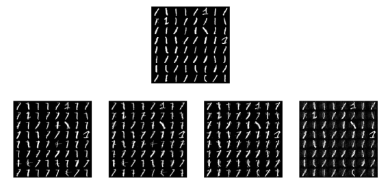
Figure 4 shows adversarial examples created on MNIST digit 1 images with attack radius . First, we observe that the perturbations added by direct attack, white-box kernel attack and black-box kernel attack are clearly targeted: either a faint horizontal stroke or a shadow of digit 7 are added to the original image. The perturbation budget is used on "key" pixels that distinguish digit 1 and digit 7, therefore the attack is effective. On the contrary, black-box attacks with neural nets substitute adds perturbation to a large number of pixels. While such perturbation often fools a neural net classifier, it is not effective against nearest neighbors. Consider a pixel that is dark in most digit 1 and digit 7 training images; adding brightness to this pixel increases the distance between the test image to training images from both classes, therefore may not change the nearest neighbor to the test image.
Figure 4 also illustrates the break-down attack radius of visual similarity. At , the true class of adversarial examples created by effective attacks becomes ambiguous even to humans. Our defense is successful as the Robust_1NN classifiers still have non-trivial classification accuracy at such attack radius. Meanwhile, we should not expect robustness against even larger attack radius since the adversarial examples at are already close to the boundary of human perception.
C.2 Training Subset Selected by Robust_1NN
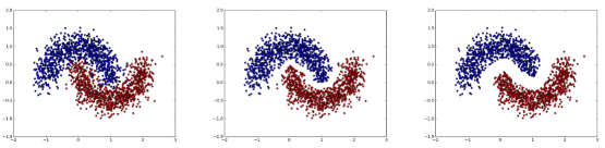
Figure 3 shows the training set selected by Robust_1NN on a halfmoon training set of size . On the original training set, we see a noisy region between the two halfmoons where both red and blue points appear. Robust_1NN cleans training points in this region so as to create a gap between the red and blue halfmoons, and the gap width increases with defense radius .
C.3 Performance of Black-box Attack Substitutes
We validate the black-box substitute training process by checking the substitute’s accuracy on its training set, the clean test set and the percentage of predictions agreeing with the target classifier on the clean test set. The results are shown in Table 1. For the halfmoon and MNIST dataset, the substitute classifiers both achieve high accuracy on both the training and test sets, and are also consistent with the target classifier on the test set. The subsitutute classifiers do not emulate the target classifier on the Abalone dataset as close as on the other two datasets due to the high noise level in the Abalone dataset. Nonetheless, the substitute classifier still achieve test time accuracy comparable to the target classifier.