Comparisons and Applications of Four Independent Numerical Approaches for Linear Gyrokinetic Drift Modes

Abstract

To help reveal the complete picture of linear kinetic drift modes, four independent numerical approaches, based on integral equation, Euler initial value simulation, Euler matrix eigenvalue solution and Lagrangian particle simulation, respectively, are used to solve the linear gyrokinetic electrostatic drift modes equation in Z-pinch with slab simplification and in tokamak with ballooning space coordinate. We identify that these approaches can yield the same solution with the difference smaller than 1%, and the discrepancies mainly come from the numerical convergence, which is the first detailed benchmark of four independent numerical approaches for gyrokinetic linear drift modes. Using these approaches, we find that the entropy mode and interchange mode are on the same branch in Z-pinch, and the entropy mode can have both electron and ion branches. And, at strong gradient, more than one eigenstate of the ion temperature gradient mode (ITG) can be unstable and the most unstable one can be on non-ground eigenstates. The propagation of ITGs from ion to electron diamagnetic direction at strong gradient is also observed, which implies that the propagation direction is not a decisive criterion for the experimental diagnosis of turbulent mode at the edge plasmas.

I Introduction and motivation

Drift modes or instabilities are micro-instabilities, driven by equilibrium non-uniformity, such as temperature and density gradients, and magnetic field non-uniformity. Those non-uniformities can lead to various particle drifts (e.g., gradient drift, curvature drift), and these particle drifts may cause particular eigen oscillation or instability, and thus these corresponding modes are called drift modes. Drift wave turbulence is considered to be the major cause for anomalous transport Horton1999 , which is an active research field in plasma physics. Thus, it is important to understand drift modes.

Gyrokinetic theory Brizard2007 , more accurate than fluid theory, is a major tool to study the low frequency ($\omega\ll\Omega_{ci}$, where $\Omega_{ci}$ is ion cyclotron frequency) drift modes. In principle, different approaches to solve the same model should give the same solution. We noticed that the discrepancy between different numerical solvers can be larger than $10\%$ (cf. Ref.Kotschenreuther1995 ; Rewoldt2007 ) for weak gradient core plasma and even larger than $50\%$ for strong gradient edge plasma (cf. Ref.Wang2012 ) in literature. We have also noticed a recent carefully verification of global gyrokinetic tokamak Euler and particle codes in Ref.Tronko2017 , where two codes GENE and ORB5 yield similar gyrokinetic models but still have visible (around 5%) deviations in real frequency and growth rate. To reveal the reasons (e.g., model difference, boundary condition difference, grids convergence, limitation of numerical approach) for this discrepancy is crucial to quantitatively study the drift modes. It also seems that no detailed benchmarks of four different approaches (based on integral equation, Euler initial value simulation, Euler eigenvalue solution and Lagrangian particle simulation, respectively) for the same gyrokinetic model are found in the literature. In this work, we use exactly the same model equation for all four approaches, in contrast to many inter-code benchmarks where both the numerics and the model equations differ to some degree. Thus, we hope this work can also be useful as a reference base, and help other researchers to choose which approach to use for their own purposes in consideration of the balance of computational time and accuracy. We have implemented all the four approaches to the code series MGK (Multi-approach GyroKinetic code).

We also find that it is very useful to understand the distribution of the linear solutions by cross checking the solutions of each approach. For example, using these four independent approaches, we apply them to reveal the relation between the interchange mode and entropy mode in Z-pinchRicci2006 and find that they are on the same branch and only one unstable mode exists in the system for small $\eta$, with $\eta=L_{n}/L_{T}$ the ratio of temperature gradient to density gradient. These approaches are also used to study the multi-eigenstates of ion temperature gradient modes coexisting in strong gradient at tokamak edge.

In the following sections, Sec.II gives the model linearized gyrokinetic equation. Sec.III gives the details of four approaches to solve the kinetic ion and electron zero-dimensional (0D) model in Z-pinch. Sec.IV extends the 0D approaches to one-dimensional (1D) model to study the ion temperature gradient mode in tokamak using kinetic ion but adiabatic electron with ballooning coordinate. Sec.V studies the drift modes under strong gradient. Sec.VI summarizes the present study.

II Gyrokinetic Linear Model

Gyrokinetic modelAntonsen1980 ; Chen1991 ; Brizard2007 can describe the low frequency physics accurately under the assumptions: $\omega/\Omega_{ci}\sim\rho_{i}/L\sim k_{\parallel}/k_{\perp}\sim\delta\ll 1$. Assuming Maxwellian equilibrium distribution function $F_{0}=n_{0}F_{M}$, $F_{M}=(\frac{m}{2\pi T})^{3/2}e^{-m\epsilon/T}$, where $\epsilon=v^{2}/2$, $v^{2}=v_{\parallel}^{2}+v_{\perp}^{2}$, $\mu=v_{\perp}^{2}/2B$, the perturbed distribution function after gyrophase average is

$$f_{\alpha}=\frac{q_{\alpha}}{m_{\alpha}}\phi\frac{\partial F^{\alpha}_{0}}{\partial\epsilon}+J_{0}(k_{\perp}\rho_{\alpha})h_{\alpha},$$ (1)

where the Bessel function of the first kind $J_{0}$ comes from gyrophase average, the non-adiabatic linearized gyrokinetic response $h_{\alpha}$ satisfies

$$(\omega-\omega_{D\alpha}+iv_{\parallel}{\bf b}\cdot{\bf\nabla})h_{\alpha}=-(\omega-\omega_{*\alpha}^{T})\frac{\partial F^{\alpha}_{0}}{\partial\epsilon}\frac{q_{\alpha}}{m_{\alpha}}J_{0}\phi.$$ (2)

Here the collision operator is neglected, and the parameters are

$$\rho_{\alpha} = \frac{v_{\perp}}{\Omega_{\alpha}},~{}~{}~{}~{}\Omega_{\alpha}=\frac{q_{\alpha}B}{m_{\alpha}c},$$

$$\frac{\partial F^{\alpha}_{0}}{\partial\epsilon} = -\frac{m_{\alpha}F_{0}^{\alpha}}{T_{\alpha}},$$

$$\omega_{*\alpha}^{T} = \frac{{\bf k}_{\perp}\times{\bf b}\cdot{\bf\nabla}F^{\alpha}_{0}}{-\Omega_{\alpha}F^{\alpha}_{0\epsilon}},$$

$$\omega_{D\alpha} = {\bf k}_{\perp}\cdot{\bf v}_{d}={\bf k}_{\perp}\cdot{\bf b}\times\frac{\mu\nabla B+v_{\parallel}^{2}{\bf b}\cdot\nabla{\bf b}}{\Omega_{\alpha}},$$

$${\bf b} = {\bf B}/B,$$

$\alpha=i,e$ represents particle species. Here, ${\bf B}$ is the magnetic field, and $q_{\alpha}$, $m_{\alpha}$, $T_{\alpha}$, $\Omega_{\alpha}$, $\rho_{\alpha}$, $\omega_{*\alpha}^{T}$ and $\omega_{D\alpha}$ are the charge, mass, temperature, cyclotron frequency, gyroradius, diamagnetic drift frequency and magnetic (gradient and curvature) drift frequency for the species $\alpha$, respectively. In electrostatic case, the quasi-neutrality condition (Poisson equation)

$$\sum_{\alpha}q_{\alpha}\int f_{\alpha}d^{3}v=0.$$ (3)

is used for field equation, where the notation for velocity integral $\int d^{3}v\equiv 2\pi\int_{-\infty}^{\infty}dv_{\parallel}\int_{0}^{\infty}v_{\perp}dv_{\perp}$, and the gyrophase average yielded $J_{0}$ has been contained in Eq.(1). In this work, we will treat both zero-dimensional (0D) model for Z-pinch and one-dimensional (1D, along field line) model for tokamak. For 1D, ${\bf b}\cdot{\bf\nabla}=\partial_{l}$; for 0D, ${\bf b}\cdot{\bf\nabla}=ik_{\parallel}$.

III Outline of Four approaches

In Z-pinch, $\omega_{*\alpha}=-\frac{cT_{0\alpha}}{q_{\alpha}Bn_{0}}\nabla n_{0}\cdot{\bm{b}}\times{\bm{k}}=k\rho_{\alpha}\frac{v_{t\alpha}}{L_{n}}$, $\omega_{d\alpha}=\frac{v_{t\alpha}^{2}}{\Omega_{c\alpha}B^{2}}{\bm{B}}\times\nabla B\cdot{\bm{k}}=k\rho_{\alpha}\frac{v_{t\alpha}}{R}=\omega_{*\alpha}L_{n}/R$, where $L_{n}^{-1}=-d\ln n_{0}/dr$, ${\bm{b}}$ being the unit vector of the magnetic field $\bm{B}$, and $q_{\alpha}$, $v_{t\alpha}=\sqrt{T_{0\alpha}/m_{\alpha}}$, $\Omega_{c\alpha}=q_{\alpha}B_{\theta}/(m_{\alpha}c)$, $m_{\alpha}$, and $\rho_{c\alpha}=v_{t\alpha}/\Omega_{c\alpha}$ being the charge, thermal velocity, cyclotron frequency, mass and gyroradius for the species $\alpha$, respectively (note $\rho_{e}<0$), $\tau=\tau_{e}=T_{0e}/T_{0i}$. For $b\ll 1$, the Bessel function $J_{0}^{2}(b)=1-b^{2}/2$. We will treat $q_{i}=-q_{e}=e$ by default. For $\tau=1$, $\omega_{*}=\omega_{*i}=-\omega_{*e}$ and $\omega_{d}=\omega_{di}=-\omega_{de}$. We also define $\kappa_{n}\equiv R/L_{n}$, $\kappa_{T}\equiv R/L_{T}$, $\epsilon_{n}\equiv L_{n}/R$ and $\eta=\kappa_{T}/\kappa_{n}$, with $L_{T}=(-d\ln T/dr)^{-1}$. One should note that: In this section, the ion diamagnetic drift frequency $\omega_{di}>0$, to be consistent with Ref.Ricci2006 ; Whereas, in the next section to study tokamak ITG mode, $\omega_{di}<0$, to be consistent with standard tokamak community notation, e.g., Ref.Dong1992 .

Figure 1: Benchmark and comparison of four approaches for entropy mode.

III.1 Integral Dispersion relation

In the 0D slab limit, the gyrokinetic model Eqs.(2) and (3) can readily be solved and yield the following integral dispersion relation

$$\sum_{\alpha}\frac{q_{\alpha}^{2}}{T_{\alpha}}\Big{\{}1-\int\frac{(\omega-\omega_{*\alpha}^{T})}{(\omega-\omega_{D\alpha}-k_{\parallel}v_{\parallel})}J_{0}^{2}F_{M\alpha}d^{3}v\Big{\}}=0,$$ (4)

where all particle species (ion and electron) are treated by gyrokinetic model. Eq.(4) is an integral equation. Without analytical continuation to $Im(\omega)\leq 0$, the above equation can only represent the $Im(\omega)>0$ growing modes correctly. The double integration $dv_{\parallel}dv_{\perp}$ can be evaluated by adaptive Simpson method. Using spectral method for $dv_{\parallel}$ Weideman1994 ; Xie2013 and Gauss-Kronrod method for $dv_{\perp}$ Gurcan2014 , the above double integration can be evaluated $\sim 200$ times faster. In practical test, we find that the Gauss method is difficult to obtain high accuracy for $\omega\to 0$ and thus is not accurate to study some parameters (especially for $k_{\perp}\rho_{i}\ll 1$ and $\gg 1$) for the entropy mode in subsection III.5. Hence, we mainly use adaptive Simpson method in this work, which is easily to control the computation precision.

Define $y=v/v_{t\alpha}$, the integral Eq.(4) is normalized to

$$\sum_{\alpha=e,i}\frac{q_{\alpha}^{2}}{T_{\alpha}}\Big{\{}1-\frac{1}{\sqrt{2\pi}}\int\frac{(\omega-\omega_{*\alpha}^{T})J_{0}^{2}(k_{\alpha}y_{\perp})}{(\omega-\omega_{D\alpha}-k_{z\alpha}v_{\parallel})}e^{-\frac{y^{2}}{2}}y_{\perp}dy_{\perp}dy_{\parallel}\Big{\}}=0,$$ (5)

with $\omega_{*\alpha}^{T}=\omega_{d\alpha}[\kappa_{n}+\kappa_{T}(y^{2}/2-3/2)]$, $\omega_{D\alpha}=\omega_{d\alpha}(y_{\parallel}^{2}+y_{\perp}^{2}/2)$, $v_{te}=v_{ti}\sqrt{\tau m_{i}/m_{e}}$, $\Omega_{e}=\frac{q_{e}m_{i}}{q_{i}m_{e}}\Omega_{i}$, $\rho_{e}=\rho_{i}\frac{q_{i}}{q_{e}}\sqrt{\tau\frac{m_{e}}{m_{i}}}$, $k_{\alpha}=k_{\perp}\rho_{\alpha}$, $k_{z\alpha}=k_{\parallel}v_{t\alpha}$. Normalized by $\omega_{0}=v_{0}/R_{0}$, with $v_{0}=v_{ti}$ and $R_{0}=R$. Thus, $\omega_{di}=k_{\perp}$, $\omega_{de}=k_{\perp}\tau\frac{q_{i}}{q_{e}}$, $k_{i}=k_{\perp}$, $k_{e}=k_{\perp}\frac{q_{i}}{q_{e}}\sqrt{\tau\frac{m_{e}}{m_{i}}}$, $k_{zi}=k_{\parallel}R$ and $k_{ze}=k_{\parallel}R\sqrt{\tau m_{i}/m_{e}}$. The dispersion relation can be solved by standard root finding approach.

III.2 Euler initial value problem

Define $g_{\alpha}(v_{\parallel},v_{\perp})=h_{\alpha}-\frac{q_{\alpha}}{T_{\alpha}}F_{0}^{\alpha}J_{0}\phi$, and using $\omega=i\partial_{t}$, we can transform the original equation to

$$\partial_{t}g_{\alpha} = -i(\omega_{D\alpha}+k_{z\alpha}y_{\parallel})g_{\alpha}-i[\omega_{D\alpha}-\omega_{T\alpha}]\phi J_{0\alpha}e^{-\frac{y^{2}}{2}},$$ (6)

$$\phi = \frac{c}{\sqrt{2\pi}}\int\Big{(}g_{i}J_{0i}+\frac{g_{e}J_{0e}}{\tau}\Big{)}y_{\perp}dy_{\perp}dy_{\parallel},$$ (7)

where $c=\frac{1}{[1-\Gamma_{0i}+(1-\Gamma_{0e})/\tau]}$, $\omega_{T\alpha}=\omega^{T}_{*\alpha}$, $J_{0\alpha}=J_{0}(k_{\alpha}y_{\perp})$, $\Gamma_{0\alpha}=I_{0}(b_{\alpha})e^{-b_{\alpha}}$, $b_{\alpha}=k_{\perp}^{2}\rho_{\alpha}^{2}=k_{\alpha}^{2}$.

The above equation can be solved as initial value problem via Euler discretization of the velocity coordinate $(v_{\parallel},v_{\perp})$. We also notice that the electron and ion can be treated in the same time scale in the above equations, since their velocities can be normalized by their own thermal velocities, i.e., $y=v/v_{t\alpha}$. This only happens when the parallel and perpendicular dynamics can be treated via the parameters $k_{\parallel}$ and $k_{\perp}$.

III.3 Euler eigenvalue problem

Eqs.(6) and (7) can also be solved as eigenvalue problem using the same Euler discretization as an initial value problem, via $\partial_{t}=-i\omega$, $\lambda X=AX$, $X=[g_{i}^{n_{y_{\parallel}}\times n_{y_{\perp}}},g_{e}^{n_{y_{\parallel}}\times n_{y_{\perp}}},\phi]^{T}$. To keep the matrix sparse, we have done a further time derivative $\partial_{t}$ on the field equation (7). This is similar to the latter 1D case Eq.(20).

We notice that this matrix eigenvalue approach may be the best approach for the present model, considering that it can give all the solutions in the system at the same time and thus will not miss solutions. This approach can be both accurate and fast for matrix dimension $N=2\times n_{y_{\parallel}}\times n_{y_{\perp}}+1\leq 5000$. Numerical results will be shown later. It should be noticed that only direct matrix solvers can give all the eigenmodes of the system. However, their execution time and memory scale with $O(N^{p})$, where usually $2.0<p\sim 2.6<3.0$. For more realistic systems (e.g. edge tokamak cases with large resolution requirements), such solvers therefore quickly become too expensive to use, and have to be replaced by iterative solvers, which will return a limited number of solutions according to a certain selection criterion. Thus, in more realistic systems, we can use low resolution to obtain all solutions and which can show the distributions of the solutions in the $\omega_{i}$ vs. $\omega_{r}$ complex plane. Then, we use the rough solution (e.g., we may be only interested in the most unstable solutions) as initial guess to obtain high resolution solution(s) via sparse matrix iterative approach, e.g., the eigs() function in MATLAB.

III.4 Particle simulation

The above model can also be solved using $\delta f$ approach Parker1993 : defining particle weight $w_{\alpha}=g_{\alpha}/F_{0}$, $F_{0}=e^{-y^{2}/2}$, initial loading $g_{\alpha}(y_{\parallel},y_{\perp},w)$ with Gaussian random number $y_{\parallel j}=randn(n_{p},1)$, $y_{\perp j}=\sqrt{randn(n_{p},1)^{2}+randn(n_{p},1)^{2}}$, and with weight being a small value, e.g., $w_{j}=10^{-6}$. Here, $n_{p}$ is particle number, $j=1,2,\cdots,n_{p}$ is particle index, and $randn()$ generates normal distribution $F_{0}=\frac{1}{\sqrt{2\pi}}e^{-x^{2}/2}$. The particle simulation evolution equations are

$$\dot{w}_{j} = -i(\omega_{D\alpha}+k_{z\alpha}y_{\parallel j})w_{j}-i[\omega_{D\alpha}-\omega_{T\alpha}]\phi J_{0}(k_{\alpha}y_{\perp}),$$ (8)

$$\phi = c\sum_{j}\Big{(}w_{ij}J_{0i}+w_{ej}J_{0e}/\tau\Big{)},$$ (9)

$\dot{y}_{\parallel j}=0$ and $\dot{y}_{\perp j}=0$.

This particle simulation approach can be seen as Monte-Carlo method, and one can refer to Ref.Aydemir1994 for the general theory and validity of it. Since this approach is based on Monte-Carlo sample, the noise level is $\sim 1/\sqrt{n_{p}}$. Thus, if we want the relative error decreasing from $10\%$ to $1\%$, we need $n^{\prime}_{p}=100n_{p}$. In this viewpoint, particle approach is not a good choice to obtain high accuracy. The benefit is that this approach is straightforward and easily coding and parallelizing.

Table 1: To converge to $\omega_{i}=0.0770$ ($\omega_{r}=0.0017$) for $k_{\perp}\rho_{i}=0.7$ with error less than $1\%$, the typical grids and computation times required.

Approach	Grids	Typical cputime
DR	accurate to $10^{-6}$	$<$1s
matrix	$n_{v_{\parallel}}=64$, $n_{v_{\perp}}=64$	$\sim$1s
ivp	$n_{v_{\parallel}}=64$, $n_{v_{\perp}}=64$, $\Delta t=0.01$, $n_{t}=10^{4}$	$\sim$5min
pic	$n_{p}=4\times 10^{5}$, $\Delta t=0.01$, $n_{t}=10^{4}$	$\sim$20min

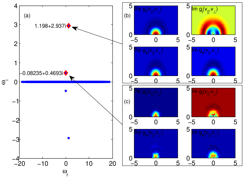
Figure 2: (a) The matrix method can give all solutions in the system. Two unstable modes exist under parameters $\eta=1.5$, $k_{\perp}\rho_{i}=0.5$, $\epsilon_{n}=0.3$, and the corresponding mode structures in velocity space are shown in (b) and (c), with $n_{v_{\parallel}}=n_{v_{\perp}}=32$. By refining the grids, the accurate values of these two solutions are $\omega=1.199+2.936i$ and $-0.019+0.471i$, which are also verified by DR method.

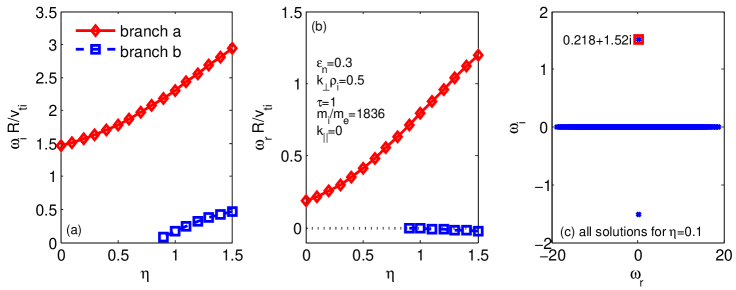
Figure 3: Scan $\eta$ for entropy mode under parameters $k_{\perp}\rho_{i}=0.5$, $\epsilon_{n}=0.3$, which shows that at $\eta>0.9$, two modes are unstable; whereas only one unstable mode for small $\eta$. (a) and (b) are obtained from DR method. (c) is from matrix method, which verifies that for $\eta=0.1$, only one unstable mode exists.

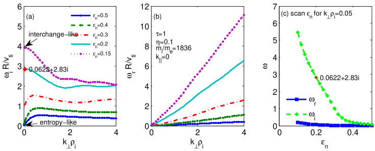
Figure 4: The entropy-like mode and interchange-like mode is on the same branch via scanning $\epsilon_{n}$.

III.5 Benchmark, comparisons of four approaches and applications

In this section, we use the mgk0d version. In the present study, all four approaches are implemented using MATLAB, and run with single core. We firstly benchmark our four approaches with the GS2 results of Fig. 4 of Ref.Ricci2006 for the entropy mode, with parameters $\eta=0$, $\tau=1$, $k_{\parallel}=0$, $\epsilon_{n}=0.95$ and $m_{i}/m_{e}=1836$. Here, entropy mode is one type of drift mode which can be unstable when macro-scale interchange mode is stable Ricci2006 . Fig.1 shows that our four approaches can be almost identical to each other, with error less than $1\%$. If we refine the grids, they can be even more close. The result is also close to Ref.Ricci2006 . Hence, we can conclude that all these four approaches can correctly study the linear physics of the gyrokinetic drift modes.

For the $k_{\perp}\rho_{i}=0.2$ case, the typical grid numbers and computation time required for each approach are listed at Table 1, where we find the most accurate and fast approach is the integral dispersion relation (DR) method, and the matrix eigenvalue approach (matrix) is also very fast and accurate. The Euler initial value (ivp) and particle (PIC) method are slow for this case, because large number of time steps $n_{t}$ is required to diagnose the complex frequency accurately. For $k_{\perp}\rho_{i}>1.5$, the grids need at least double to make sure the error less than $1\%$, and thus the computation times for both approaches are usually larger than 1hr.

Dispersion relation can only give the complex frequency $\omega$, whereas the other three approaches can also give the structure of $g(v_{\parallel},v_{\perp})$ directly, which can help to show the resonance structure in the phase space. To calculate the mode structure of $g(v_{\parallel},v_{\perp})$ in DR method, one needs to plug the solution back into the equation for the distribution function. Particle simulation and initial value simulation can also easily study the most weakly damped mode (see next section for 1D case). The matrix method can not represent the damping mode correctly. We will show these features step by step. Since DR and matrix methods are both fast and accurate, we will mainly use these two approaches for the following studies.

The purpose of the present work is not merely to show that four approaches can give the same solution, but to help to reveal the unclear physics when single approach is not sufficient to draw a conclusion. Now, we begin to show a more complete picture of entropy mode, i.e., how many unstable solutions exist, ion mode or electron mode, what is the relationship with interchange mode.

Firstly, we show all solutions in the system via matrix eigenvalue method. For $\eta=1.5$, $\tau=1$, $k_{\parallel}=0$, $\epsilon_{n}=0.3$ $k_{\perp}\rho_{i}=0.5$ and $m_{i}/m_{e}=1836$, all solution in the system is shown in Fig.2a. We find that only two unstable modes exist and one is in ion diamagnetic direction and one is in electron diamagnetic direction, i.e., there exist two types of entropy mode. And we call them ion mode and electron mode respectively. In Fig.2b and c, we can find that the phase space structure is wider for ion mode and narrow for electron mode by comparison with their thermal velocities. Fig.3a and b shows more clearly of the two branches. And for large $\eta_{i}>\eta_{c}$, two modes can coexist; whereas for small $\eta$, only electron mode exists. Fig.3c confirms that for $\eta_{i}=0.1$, only one unstable mode exists in the system. The critical gradient $\eta_{c}$ is around $2/3$. In this aspect, the ion entropy mode is similar to ion temperature gradient mode (ITG) in tokamak which is unstable at larger $\eta_{i}$; and electron entropy mode is electron drift mode which can be driven to be unstable by density gradient alone.

Secondly, we try to understand the relationship of entropy mode and interchange mode. Usually, the interchange mode and entropy mode are considered to be two different modes (cf. Ref.Ricci2006 ), because of their different behaviors in parameters space: For $k_{\parallel}=0$ and $k_{\perp}\to 0$, the local interchange mode $\gamma\to\gamma_{0}\neq 0$; whereas the entropy mode $\gamma\to 0$. If this is the case, there should be a parameter range that both modes are unstable or the transition from one mode to another in parameter space should be non-smooth. Entropy mode is considered to be driven to become unstable by pressure gradient when magnetohydrodynamic interchange mode is stable. Thus, we scan the gradient parameter $\epsilon_{n}$. In Fig.4a, we find that indeed an interchange-like mode exists for $\epsilon_{n}\leq 0.2$ and an entropy-like mode exists for $\epsilon_{n}\geq 0.4$. However, in Fig.4c, via scanning of $\epsilon_{n}$ at small $k_{\perp}\rho_{i}=0.05$, we find the transition between these two types of mode are smooth, i.e., they are in the same branch. This also agrees with our previous study (Fig.3) that for small $\eta_{i}$, only one unstable mode exists in the system, either ‘interchange-like’ or ‘entropy-like’.

In summary, different numerical approaches can yield the same solution at convergent limit, but each approach has their own advantages and disadvantages. DR method is fast but requires good initial guess and can not give phase space structure directly; IVP and PIC are slow but can simulate damped mode directly. Matrix method is the best method for the present study, which can give all solution in the system and are also fast. However, matrix method can not treat damped mode correctly, which is probably because damped mode is the combination of Case-van Kampen modes and not a real eigenmode (cf. Ref.Xie2013b and references in for more detailed discussions). Combination of multi-approaches can help to cross check each other and can help to reveal unclear physics in single approach, as shown by the two examples above.

IV Extension to 1D

In this section, we treat the 1D toroidal ion temperature gradient mode (ITG). The electron is assumed adiabatic $h_{e}=0$.

We focus on the linearized electrostatic gyrokinetic ITG equation in ballooning space, ${\bf b}\cdot{\bf\nabla}=\partial_{l}=\frac{1}{qR}\frac{\partial}{\partial\theta}$, where $\theta$ is the ballooning angle coordinate. The gyrokinetic equation changes to Dong1992 :

$$\frac{iv_{\parallel}}{qR}\frac{\partial}{\partial\theta}h+(\omega-\omega_{D})h = (\omega-\omega_{*T})J_{0}(\beta)F_{M}\frac{en_{0i}}{T_{i}}\phi(\theta),$$ (10)

$$(1+1/\tau_{e})\frac{en_{0i}}{T_{i}}\phi = \int d^{3}vJ_{0}(\beta)h,$$ (11)

where $\beta=k_{\perp}v_{\perp}/\Omega_{ci}$, $q_{i}=-q_{e}=e$, $b_{i}=k_{\perp}^{2}\rho_{ti}^{2}$, $\rho_{ti}=v_{ti}/\Omega_{ci}$, $v_{ti}=(T_{i}/m_{i})^{1/2}$, $\Omega_{ci}=eB/m_{i}c$, $h$ is non-adiabatic response of ion, $\omega_{*T}=\omega_{*i}\{1+\eta_{i}[v_{\perp}^{2}/(2v_{ti}^{2})+v_{\parallel}^{2}/(2v_{ti}^{2})-3/2]\}$, $\omega_{D}=2\epsilon_{n}\omega_{*i}[\cos\theta+s(\theta-\theta_{k})\sin\theta](v_{\perp}^{2}/2+v_{\parallel}^{2})/(2v_{ti}^{2})$, $\omega_{*i}=-(ck_{\theta}T_{i})/(eBL_{n})$, $L_{n}=-(d\ln n/dr)^{-1}$, $\eta_{i}=L_{n}/L_{T_{i}}$, $\tau_{e}=T_{e}/T_{i}$, $s=(r/q)(dq/dr)$, $F_{M}=(\frac{m_{i}}{2\pi T_{i}})^{3/2}e^{-m_{i}v^{2}/2T_{i}}$, $k_{\perp}^{2}=k_{\theta}^{2}[1+s^{2}(\theta-\theta_{k})^{2}]$. $\theta_{k}$ is ballooning angle parameter. We consider only passing particles, with also $v_{\parallel}$ unchanged along the field line.

Normalization: ${\hat{\omega}}=\omega/\omega_{0}$, $\omega_{0}=v_{0}/r_{0}$, $v_{0}=v_{ti}$, $r_{0}=R$. ${\hat{k}}=k\rho_{ti}$, ${\hat{v}}=v/v_{ti}$. ${\hat{\phi}}=e\phi/T_{i}$, ${\hat{h}}=hv_{ti}^{3}/n_{0i}$. In the below, we omit the hat symbol. The normalized equation is

$$\frac{iv_{\parallel}}{q}\frac{\partial}{\partial\theta}h+(\omega-\omega_{D})h = (\omega-\omega_{*T})J_{0}(\beta)F_{M}\phi(\theta),$$ (12)

$$(1+1/\tau_{e})\phi = \int d^{3}vJ_{0}(\beta)h,$$ (13)

where $\beta=k_{\perp}v_{\perp}$, $b_{i}=k_{\perp}^{2}$, $\omega_{*T}=\omega_{*i}[1+\eta_{i}(v_{\perp}^{2}+v_{\parallel}^{2}-3)/2]$, $\omega_{D}=\omega_{di}[\cos\theta+s(\theta-\theta_{k})\sin\theta](v_{\perp}^{2}/2+v_{\parallel}^{2})$, $\omega_{*i}=-k_{\theta}/\epsilon_{n}$, $\omega_{di}=-k_{\theta}$ and $F_{M}=(2\pi)^{-3/2}e^{-v^{2}/2}$, $\int d^{3}v=2\pi\int_{-\infty}^{\infty}dv_{\parallel}\int_{0}^{\infty}v_{\perp}dv_{\perp}$.

IV.1 Integral Dispersion relation

For completeness, in this subsection, we outline the derivation of integral equation of the solution to the Eqs.(12) and (13). As from Eq.(12)

$$\frac{\partial}{\partial\theta}\Big{[}h\exp\Big{(}-i\int^{\theta}d\theta^{\prime}(\omega-\omega_{D})\frac{q}{v_{\parallel}}\Big{)}\Big{]}=-iF_{M}$$

$$\frac{q}{v_{\parallel}}J_{0}(\omega-\omega_{*T})\delta\phi(\theta)\exp\Big{(}-i\int^{\theta}d\theta^{\prime}(\omega-\omega_{D})\frac{q}{v_{\parallel}}\Big{)},$$

we can obtain

$$h^{+}(\theta)=-i\int_{-\infty}^{\theta}d\theta^{\prime}F_{M}\frac{q}{|v_{\parallel}|}J_{0}(\omega-\omega_{*T})\delta\phi(\theta^{\prime})\exp(-iI_{\theta}^{\theta^{\prime}}),$$

and

$$h^{-}(\theta)=-i\int_{\theta}^{\infty}d\theta^{\prime}F_{M}\frac{q}{|v_{\parallel}|}J_{0}(\omega-\omega_{*T})\delta\phi(\theta^{\prime})\exp(+iI_{\theta}^{\theta^{\prime}}),$$

where

$$I_{\theta}^{\theta^{\prime}}=\int_{\theta}^{\theta^{\prime}}d\theta^{\prime\prime}(\omega-\omega_{D})\frac{q}{|v_{\parallel}|}.$$

Or, we combine the $h^{+}$ and $h^{-}$

$$h(v_{\parallel}>0)+h(v_{\parallel}<0)=-i\int_{-\infty}^{\infty}d\theta^{\prime}F_{M}\frac{q}{|v_{\parallel}|}$$

$$J_{0}(\beta^{\prime})(\omega-\omega_{*T})\delta\phi(\theta^{\prime})\exp\Big{[}i\int_{\theta^{\prime}}^{\theta}d\theta^{\prime\prime}(\omega-\omega_{D})\frac{qS}{|v_{\parallel}|}\Big{]},$$

where $S\equiv sign(\theta-\theta^{\prime})$. And thus the following Fredholm integral equation is obtained via substituting the above solution of $h$ in to the field equation (13)

$$L\delta\phi(\theta)\equiv(1+\tau)\delta\phi(\theta)-\int_{0}^{\infty}dv_{\parallel}\int_{0}^{\infty}dv_{\perp}\int_{-\infty}^{\infty}d\theta^{\prime}K_{0}=0,$$ (14)

$$K_{0}(v_{\parallel},v_{\perp},\theta,\theta^{\prime},\omega)\equiv-2\pi iv_{\perp}\tau\frac{q}{|v_{\parallel}|}(\omega-\omega_{*T})$$

$$J(\beta^{\prime})J(\beta)F_{0}\delta\phi(\theta^{\prime})\exp\Big{[}i\int_{\theta^{\prime}}^{\theta}d\theta^{\prime\prime}\frac{\omega-\omega_{D}}{|v_{\parallel}|}qS\Big{]},$$

with boundary condition $\delta\phi\to 0$ at $\theta\to\pm\infty$, and

$$\int_{\theta^{\prime}}^{\theta}d\theta^{\prime\prime}\frac{\omega-\omega_{D}}{|v_{\parallel}|}qS=\frac{\omega}{|v_{\parallel}|}q|\theta-\theta^{\prime}|-\frac{\omega_{di}}{|v_{\parallel}|}q(v_{\perp}^{2}/2+v_{\parallel}^{2})$$

$$~{}~{}~{}~{}~{}~{}S[(1+s)\sin\theta^{\prime\prime}+s(\theta_{k}-\theta^{\prime\prime})\cos\theta^{\prime\prime}]\Big{|}_{\theta^{\prime}}^{\theta}.$$

The above derivation is similar to Ref.Romanelli1989 and Lu2017 .

In numerical aspect, we use Ritz method via basis functions expansion

$$\delta\phi(\theta) = \sum_{m}\delta\phi_{m}h_{m}(\theta-\theta_{c}),$$

$$h_{m}(\theta) = \exp[-(c_{1}\theta)^{2}/2]H_{m}(c_{1}\theta)\sqrt{\frac{c_{1}}{2^{m}m!\sqrt{\pi}}},$$

where $c_{1}$ and $\theta_{c}$ are adjustable parameters,

$$\int_{-\infty}^{\infty}dxh_{m}(x)h_{m^{\prime}}(x)=\delta_{mm^{\prime}}$$

and $H_{m}$ is the $m$-th Hermite polynomial, i.e.,

$$H_{0}(x)=1,~{}~{}H_{1}(x)=2x,$$

$$H_{2}(x)=4x^{2}-2,~{}~{}H_{3}(x)=8x^{3}-12x,~{}~{}\cdots$$

Thus, Eq.(12) is solved as matrix eigenvalue problem

$$M_{mm^{\prime}}\delta\phi_{m}=0,$$ (15)

$$M_{mm^{\prime}}=(1+\tau)\delta_{mm^{\prime}}-\int_{-\infty}^{\infty}d\theta h_{m^{\prime}}(\theta)\int_{0}^{\infty}dv_{\parallel}\int_{0}^{\infty}dv_{\perp}\int_{-\infty}^{\infty}d\theta^{\prime}K_{0}.$$ (16)

The above approach is also used in FULL codeRewoldt1982 and Ref.Lu2017 , whereas HD7Dong1992 code use a rectangle and triangle basis functions.

IV.2 Euler initial value problem

Define $g(\theta,v_{\parallel},v_{\perp})\equiv h(\theta,v_{\parallel},v_{\perp})-J_{0}(\beta)F_{M}(v_{\parallel},v_{\perp})\phi(\theta)$, and use $\omega=i\partial_{t}$, we obtain

$$\partial_{t}g = -\frac{v_{\parallel}}{q}[\partial_{\theta}g+J_{0}F_{M}\partial_{\theta}\phi+(\partial_{\theta}J_{0})F_{M}\phi]$$ (17)

$$-i\omega_{D}g+i(\omega_{*T}-\omega_{D})J_{0}F_{M}\phi,$$

$$\phi = \frac{1}{(1+1/\tau_{e}-\Gamma_{0})}\int d^{3}vJ_{0}g,$$ (18)

where $\Gamma_{0}=I_{0}(b_{i})e^{-b_{i}}$, and $I_{0}$ is the modified Bessel function. And $\partial_{\theta}J_{0}=-J_{1}(\beta)k_{\theta}v_{\perp}s^{2}(\theta-\theta_{k})/\sqrt{1+s^{2}(\theta-\theta_{k})^{2}}$, since $J_{0}^{\prime}(x)=-J_{1}(x)$. This approach is similar to GS2 Kotschenreuther1995 code.

IV.3 Euler eigenvalue problem

With Euler discretization to eigen matrix and $\lambda=\partial_{t}=-i\omega$, we obtain

$$\omega g = -i\frac{v_{\parallel}}{q}[\partial_{\theta}g+J_{0}F_{M}\partial_{\theta}\phi+(\partial_{\theta}J_{0})F_{M}\phi]$$ (19)

$$+\omega_{D}g-(\omega_{*T}-\omega_{D})J_{0}F_{M}\phi,$$

$$\omega\phi = \frac{1}{(1+1/\tau_{e}-\Gamma_{0})}\int d^{3}vJ_{0}\omega g,$$ (20)

The $\omega g$ in the integral of Eq.(20) is replaced by the right hand side of Eq.(19), and yields

$$\int d^{3}vJ_{0}\omega g=2\pi\int_{-\infty}^{\infty}dv_{\parallel}\int_{0}^{\infty}v_{\perp}dv_{\perp}J_{0}[-i\frac{v_{\parallel}}{q}\partial_{\theta}g+\omega_{D}g]$$

$$+\{\omega_{di}f_{d}[(2-b_{i})\Gamma_{0}+b_{i}\Gamma_{1}]-\omega_{*i}[(1-b_{i}\eta_{i})\Gamma_{0}+b_{i}\eta_{i}\Gamma_{1}]\}\phi,$$

where $f_{d}=\cos\theta+s(\theta-\theta_{k})\sin\theta$. The eigenvalue problem is $\omega X=MX$, where $X=[g(\theta,v_{\parallel},v_{\perp}),\phi(\theta)]$. For the central difference of $\partial_{\theta}$, we noticed that high order finite difference is required, e.g., we find the 4th order coefficients $(1/12,-2/3,0,2/3,-1/12)$ for $\phi_{j-2,j-1,j,j+1,j+2}$ is much better than the 2nd order coefficients $(-1/2,0,1/2)$ for $\phi_{j-1,j,j+1}$.

IV.4 Particle simulation

The 1D model can also be solved via particle simulation. Defining the $\delta f$ weight $w=g/F_{M}$, the gyrokinetic system changes to

$$\frac{d\theta}{dt}=\frac{v_{\parallel}}{q},$$ (21)

$$\frac{dw}{dt} = -i\omega_{D}w+i(\omega_{*T}-\omega_{D})J_{0}\phi-$$ (22)

$$\frac{v_{\parallel}}{q}[J_{0}\partial_{\theta}\phi+(\partial_{\theta}J_{0})\phi],$$

$$\Big{(}1+\frac{1}{\tau_{e}}-\Gamma_{0}\Big{)}\phi=\int J_{0}gd^{3}v.$$ (23)

The simulation steps (here $j=1,2,\cdots,n_{p}$ is particles index, and $n_{p}$ is the total particle number) are:

• 1. Loading particles, $\theta$ uniform $rand(np)$, $v_{\parallel}$ Maxwellian $randn(np)\times v_{t}$, the perpendicular velocity should be careful $v_{\perp}=\sqrt{randn(np)^{2}+randn(np)^{2}}\times v_{t}$;

• 2. Calculating $k_{\perp}v_{\perp}$, $\omega_{*T}$, $\omega_{D}$ for each particle $j$;

• 3. Push particles $\theta_{j}$, update $w_{j}$ for each particle;

• 4. Calculating $\phi(\theta)$, with $J_{0}$ and $\partial_{\theta}(J_{0})$, $\int J_{0}g_{i}dv^{3}$;

• 5. Back to step 2.

This approach is similar to the approach in Ref.Zhao2002 and AWECS Bierwage2008 code.

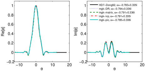
Figure 5: Benchmark and comparisons of four approaches with Ref.Dong1992 ITG solution. Both complex frequency and mode structure are close to each other.

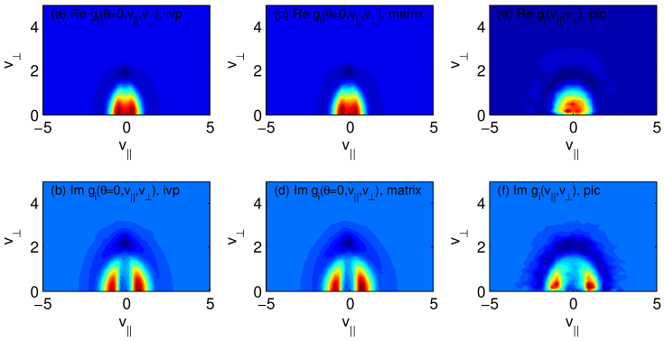
Figure 6: Comparisons of $g_{i}(v_{\parallel},v_{\perp})$ with the same case of Fig.5.

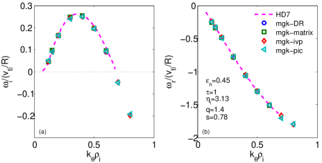
Figure 7: Benchmark and comparisons of four approaches with the Cyclone parameters.

Table 2: Typical grids and cpu time for mgk1d.

Approach	Grids	Typical cputime
DR	$n_{\theta}=400$, $n_{M}=25$, $n_{v_{\parallel}}=31$, $n_{v_{\perp}}=31$	$\sim$5min
matrix	$n_{\theta}=200$, $n_{v_{\parallel}}=32$, $n_{v_{\perp}}=32$	$\sim$1min
ivp	$n_{\theta}=128$, $n_{v_{\parallel}}=64$, $n_{v_{\perp}}=64$, $\Delta t=0.01$, $n_{t}=10^{3}$	$\sim$30min
pic	$n_{\theta}=128$, $n_{p}=4\times 10^{5}$, $\Delta t=0.01$, $n_{t}=10^{3}$	$\sim$30min

IV.5 Benchmark and comparisons

We benchmark the present solvers with Ref.Dong1992 , which is also based on integral method. However, the equation solved in Ref.Dong1992 has adopted analytical integral along $v_{\perp}$ and modified the integral $dv_{\parallel}$. It is not clear whether the latter step will affect the final solution. The parameters are: $k_{\perp}\rho_{i}=0.45/\sqrt{2}$, $s=q=\tau=1.0$, $\epsilon_{n}=0.25$, $\eta_{i}=2.5$. The original data in Dong1992 is $\omega^{Dong92}=(-0.607+0.258i)\omega_{se}=-0.773+0.328i$. The newly calculated with fine grids using the same solver HD7 gives $\omega^{HD7}=(-0.615+0.263i)\omega_{se}=-0.783+0.335i$. The results are shown in Fig.5, where we can find that four approaches and HD7 results agree very well with difference smaller than $1\%$ for both complex frequency and mode structure.

The velocity space structure $g_{i}(v_{\parallel},v_{\perp})$ of three approaches are shown in Fig.6. We can find that IVP and matrix are almost the same, whereas PIC is also similar but not exactly the same. This is probably because we gather all the particles not only just around $\theta=0$ in the PIC method, whereas in IVP and matrix method we only plot $g_{i}(\theta=0)$. Another reason may be the particle noise, since only $n_{p}=1.6\times 10^{5}$ particles are used. The typical computation grids and cpu time are shown in 2. We find in this 1D case, matrix method is the most fast and accurate approach. And the DR method is not the fastest method any more which can mainly due to the quadruple integral. And thus matrix method will be our prior choice.

Next, we benchmark the well known Cyclone case parameters: $s=0.78$, $q=1.4$, $\tau=1$, $\eta_{i}=3.13$, $\epsilon_{n}=0.45$. The results are shown in Fig.7. We can find that four approaches can also agree well. The IVP and PIC method can be more close to the matrix method when we use more grids or particles. However, we noticed a slight ($\sim 7\%$) discrepancy of the growth rate between mgk and HD7 at $k_{\theta}\rho_{i}\geq 0.4$. The reason is not clear yet, which is probably due to round off error of mgk-matrix, particle noise of mgk-pic, grid convergence of mgk-dr and mgk-ivp, or the grid convergence in HD7, especially the velocity space integral of HD7 using Gauss method which may be difficult to be high accuracy. We have also tested the MPI parallelized Fortran version of mgk1d-pic for $k_{\theta}\rho_{i}=0.6$, the convergent result with up to $n_{p}=6.4\times 10^{5}$ particles is $\omega=-1.51+0.089i$, close to the one in Fig.7, whereas $\omega^{\rm HD7}=-1.50+0.105i$.

The ITG is damped at $k_{\theta}\rho_{i}>0.7$ as shown in Fig.7a via IVP and PIC method. We further shown a typical mode structure of this damped mode in Fig.8 with $k_{\theta}\rho_{i}=0.8$, which is simulated by IVP. And the PIC method shows similar result. Damped ITG is studied at Ref.Sugama1999 via integral method, where careful treatment of the analytical continuation is required.

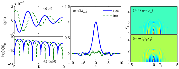
Figure 8: For cyclone parameters, the $k_{\perp}\rho_{i}=0.8$ mode is damped, which can be seen in ivp simulation.

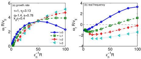
Figure 9: At strong gradient, the most unstable ITG mode transits from even mode of $l=0$ ground state to $l\geq 1$ high order ITG modes at $\epsilon_{n}^{-1}R\simeq 50$. Note also the change of the direction of the real frequency from ion direction to electron direction.

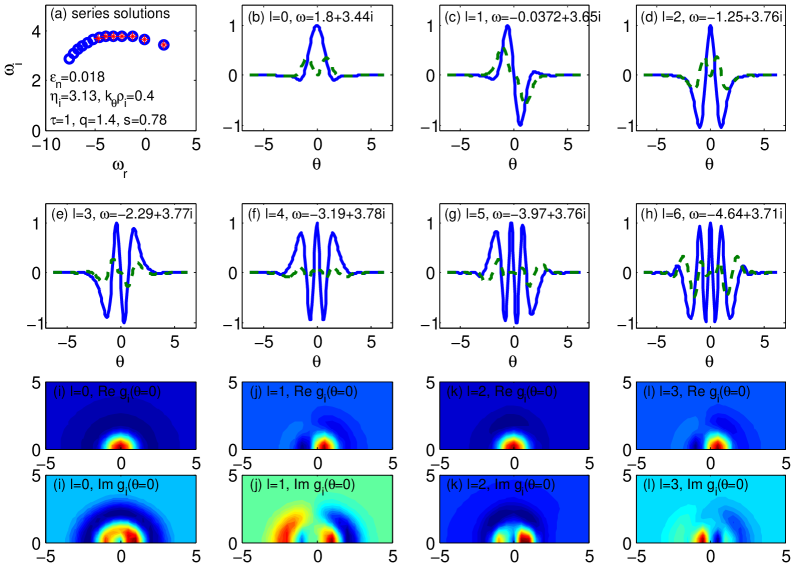
Figure 10: For cyclone parameters, $k_{\perp}\rho_{i}=0.4$ and $\epsilon_{n}=0.018$. Multi-eigenmodes are shown, where the most unstable modes are around quantum number $l\simeq 2-5$. Matrix method, which is both fast and accurate under this parameter.

V Strong gradient ITGs

The above four approaches can have various applications, since we solve the original gyrokinetic model with no approximation and have verified that they can yield the same solution. In this work, we focus on strong gradient, where very interesting new physics are expected Xie2017 . Especially, we hope to understand more of the multi eigenstates at tokamak edge Xie2015 ; Xie2016 ; Han2017 , where more than one unstable ITGs or trapped electron modes (TEMs) represent different eigenstates (we will label them by quantum number ‘$l$’) are found under particular physical parameters.

We still use the Cyclone parameters but change gradient parameter $\epsilon_{n}$, where we find multi-eigenstates coexist, as shown in Fig.9. In this section, we mainly use matrix method, since IVP and PIC methods are difficult to separate multi-modes with close growth rate and strongly depend on initial setups and thus we have not shown their results here. The DR method requires large grids to converge. And we have checked that the DR method can converge to the matrix result via increasing grids. We can find that the $l=0$ ground state ITG mode is no longer the most unstable one at around $\epsilon_{n}^{-1}>50$. The growth rate of the ground state mode increases and then decreases, and the real frequency of it transits from ion to electron diamagnetic direction at around $\epsilon_{n}^{-1}>20$. This is not clearly found by the systematically parameters scan in Ref.Han2017 via HD7 code. One reason is that HD7 requires well initial guess. From the above result, under Cyclone parameters and $k_{\theta}\rho_{i}=0.4$, at the range $20<\epsilon_{n}^{-1}<50$, the most unstable ITG mode is on the ground state but propagates at electron diamagnetic direction. This new feature tells us that the propagation direction is not a decisive criterion of the mode for the experimental diagnosis of turbulence at the edge plasmas.

In Fig.9, we also noticed that ITGs transition is not a sudden transition, but several modes with similar growth rates are most unstable at almost the same critical gradient. This may also explain why the global gyrokinetic PIC simulation in Ref.Xie2015 for high order ITG modes does not have clear mode structures, whereas the TEMs simulation can separate well. This feature also leads difficulties for IVP and PIC to clearly study the multi-eigenstates of ITGs.

We show series solutions of ITGs under the same Cyclone parameters with $\epsilon_{n}=0.018$ via matrix method in Fig.10. Artificial solutions with non-smooth mode structures and higher order solutions have been removed in Fig.10a. We find the most unstable mode under this parameter is $l\simeq 2-5$, and the mode structures of $\phi(\theta)$ of $l=0-6$ are shown in Fig.10b-h. Figure10i-l show the velocity space structures of $l=0-3$. We can find that the mode structures of $g_{i}(v_{\parallel},v_{\perp})$ in different eigenstates $l$ are also different, and especially the odd modes and even modes are of different types. How to reveal the physical mechanism and the transitions of the modes through the linear solution $\omega$, $\phi(\theta)$ and $g_{i}(\theta,v_{\parallel},v_{\perp})$ is out of the scope of present work.

VI Summary and Conclusion

In summary, the present work makes new conclusions regarding ITG modes in strong gradients along with the development of four new computational tools for gyro-kinetic simulation of magnetized plasma. We have developed four independent approaches, based on integral dispersion relation, Euler initial value simulation, Euler matrix eigenvalue solution, and Lagrangian particle simulation, respectively, to study the linear gyrokinetic drift modes. We identify that these four approaches can yield the same solution and the differences mainly come from the convergence. These provide a good tool to study the complete picture of linear drift modes. For example, using these methods, we find that entropy mode has both electron and ion branches, and the transition between interchange mode and entropy mode is a smooth transition and we can consider them as the same mode. Using matrix method, all solutions in the system can be revealed and thus we can easily know the distributions and transitions of the modes in the system. The multi-eigenstates of gyrokinetic ITG can be seen such clearly for the first time, via matrix method. Most importantly, we find that the propagation direction is not a decisive criterion for the experimental diagnosis of turbulent mode at the edge plasmas, i.e., the most unstable ITG can propagate at electron direction!

In conclusion, this work, providing four tools, can have many potential applications in the future to reveal different aspects of linear kinetic mirco-instabilities. Examples of applications to strong gradient to reveal new physics are shown for both Z-pinch entropy mode and tokamak ITGs. Electromagnetic, collision and trapped particle effects can be added in principle. The performance comparisons in the present work is rather crude, which is mainly due to that it is difficult to determined the computation precision and thus it may not be fair for the comparisons. Both IVP and PIC methods scales linearly to the grids/particle numbers. The performance of the iterative solver of matrix and DR methods depends on both grid numbers and initial guess. And also, optimizations of each codes to speed up are possible and can be considered as future works. We should also emphasize that although the above four approaches have outlined the major linear methods, the implementations can be varying, examples including GENERoman2010 , GYROBelli2010 , LIGKALauber2007 , etc.

Appendix A Useful integrals

Some useful integrals

$$\int_{0}^{\infty}x^{2n}e^{-x^{2}/a^{2}}dx=\frac{a^{2n+1}(2n-1)!!}{2^{n+1}}\sqrt{\pi},$$

$$\int_{0}^{\infty}x^{2n+1}e^{-x^{2}/a^{2}}dx=\frac{n!}{2}a^{2n+2},$$

$$\int_{0}^{\infty}xe^{-x^{2}/2}J_{p}^{2}(\sqrt{b_{s}}x)dx=e^{-b_{s}}I_{p}(b_{s}),$$

$$\int_{0}^{\infty}x^{3}e^{-x^{2}/2}J_{p}^{2}(\sqrt{b_{s}}x)dx=2e^{-b_{s}}[$$

$$~{}~{}~{}~{}~{}~{}~{}~{}~{}~{}(1-b_{s}+p)I_{p}(b_{s})+b_{s}I_{p+1}(b_{s})],$$

where $J_{p}$ and $I_{p}$ are Bessel and modified Bessel functions, respectively.

References

- (1) W. Horton, Rev. Mod. Phys., 71, 735 (1999).
- (2) A. J. Brizard and T. S. Hahm, Rev. Mod. Phys., 79, 421 (2007).
- (3) M. Kotschenreuther, G. Rewoldt and W. Tang, Computer Physics Communications, 88, 128 (1995).
- (4) G. Rewoldt, Z. Lin and Y. Idomura, Computer Physics Communications, 177, 775 (2007).
- (5) E. Wang, X. Xu, J. Candy, R. Groebner, P. Snyder, Y. Chen, S. Parker, W. Wan, G. Lu, and J. Dong, Nucl. Fusion, 52, 103015 (2012).
- (6) N. Tronko, A. Bottino, T. Gorler, E. Sonnendrucker, D. Told and L. Villard, Phys. Plasmas, 24, 056115 (2017).
- (7) P. Ricci, B. N. Rogers, W. Dorland, and M. Barnes, Phys. Plasmas, 13, 062102 (2006).
- (8) T. M. Antonsen and B. Lane, Phys. Fluids 23, 1205 (1980).
- (9) L. Chen and A. Hasegawa, Journal Of Geophysical Research, 96, 1503 (1991).
- (10) J. Q. Dong, W. Horton and J. Y. Kim, Phys. Fluids B, 4, 1867 (1992).
- (11) H. S. Xie, Phys. Plasmas, 20, 092125 (2013).
- (12) J. A. C. Weideman, SIAM J. Numer. Anal. 31, 1497 (1994).
- (13) O. Gurcan, Journal of Computational Physics, 269, 156 (2014).
- (14) S. E. Parker and W. W. Lee, Physics of Fluids B: Plasma Physics, 5, 77 (1993).
- (15) A. Y. Aydemir, Physics of Plasmas, 1, 822-831 (1994).
- (16) H. S. Xie, Phys. Plasmas, 20, 112108 (2013).
- (17) F. Romanelli, Physics of Fluids B, 1, 1018 (1989).
- (18) Z. X. Lu, E. Fable, W. A. Hornsby, C. Angioni, A. Bottino, Ph. Lauber and F. Zonca, Phys. Plasmas, 24, 042502 (2017).
- (19) G. Rewoldt, W. M. Tang and M. S. Chance, Physics of Fluids, 25, 480 (1982).
- (20) G. Zhao and L. Chen, Phys. Plasmas, 9, 861 (2002).
- (21) A. Bierwage and L. Chen, Commun. Comput. Phys., 4, 457 (2008).
- (22) H. S. Xie, Y. Xiao and Z. Lin, Phys. Rev. Lett., 118, 095001 (2017).
- (23) H. S. Xie and Y. Xiao, Phys. Plasmas, 22, 090703 (2015).
- (24) H. S. Xie and B. Li, Phys. Plasmas, 23, 082513 (2016).
- (25) M. K. Han, Z. X. Wang, J. Q. Dong and H. R. Du, Nucl. Fusion, 57, 046019 (2017).
- (26) H. Sugama, Phys. Plasmas, 6, 3527 (1999).
- (27) J. E. Roman, M. Kammerer, F. Merz and F. Jenko, Parallel Computing, 36, 339 (2010).
- (28) E. A. Belli and J. Candy, Phys. Plasmas, 17, 112314 (2010).
- (29) P. Lauber, S. Gunter, A. Konies and S. D. Pinches, Journal of Computational Physics, 226, 447 (2007).