A New Probabilistic Algorithm for Approximate Model Counting

Abstract

Constrained counting is important in domains ranging from artificial intelligence to software analysis. There are already a few approaches for counting models over various types of constraints. Recently, hashing-based approaches achieve both theoretical guarantees and scalability, but still rely on solution enumeration. In this paper, a new probabilistic polynomial time approximate model counter is proposed, which is also a hashing-based universal framework, but with only satisfiability queries. A variant with a dynamic stopping criterion is also presented. Empirical evaluation over benchmarks on propositional logic formulas and SMT(BV) formulas shows that the approach is promising.

1 Introduction

Constrained counting, the problem of counting the number of solutions for a set of constraints, is important in theoretical computer science and artificial intelligence. Its interesting applications in several fields include probabilistic inference [25, 10], planning [12], combinatorial designs and software engineering [23, 15]. Constrained counting for propositional formulas is also called model counting, to which probabilistic inference is easily reducible. However, model counting is a canonical #P-complete problem, even for polynomial-time solvable problems like 2-SAT [31], thus presents fascinating challenges for both theoreticians and practitioners.

There are already a few approaches for counting solutions over propositional logic formulas and SMT(BV) formulas. Recently, hashing-based approximate counting achieves both strong theoretical guarantees and good scalability [24]. The use of universal hash functions in counting problems began in [28, 30], but the resulting algorithm scaled poorly in practice. A scalable approximate counter ApproxMC in [8] scales to large problem instances, while preserves rigorous approximation guarantees. ApproxMC has been extended to finite-domain discrete integration, with applications to probabilistic inference [13, 5, 2], and improved by designing efficient universal hash functions [19, 6] and reducing the use of NP-oracle calls from linear to logarithmic [9].

The basic idea in ApproxMC is to estimate the model count by randomly and iteratively cutting the whole space down to a small “enough” cell, using hash functions, and sampling it. The total model count is estimated by a multiplication of the number of solutions in this cell and the ratio of whole space to the small cell. To determine the size of the small cell, which is essentially a small-scale model counting problem with the model counts bounded by some thresholds, a model enumeration in the cell is adopted. In previous works, the enumeration query was handled by transforming it into satisfiability queries, which is much more time-consuming than a single satisfiability query. An algorithm called MBound [17] only invokes satisfiability query once for each cut. Its model count is determined with high precision by the number of cuts down to the boundary of being unsatisfiable. However, this property is not strong enough to give rigorous guarantees, and MBound only returns an approximation of upper or lower bound of the model count.

In this paper, a new hashing-based approximate counting algorithm, with only satisfiability query, is proposed, building on a correlation between the model count and the probability of the hashed formula being unsatisfiable. Dynamic stopping criterion for the algorithm to terminate, once meeting the theoretical guarantee of accuracy, are presented. Like previous works, a theoretical termination bound $T$ is shown. Theoretical insights over the efficiency of a prevalent heuristic strategy called leap-frogging are also provided.

The proposed approach is a general framework easy to handle various types of constraints. Prototype tools for propositional logic formulas and SMT(BV) formulas are implemented. An extensive evaluation on a suite of benchmarks demonstrates that (i) the approach significantly outperforms the state-of-the-art approximate model counters, including a counter designed for SMT(BV) formulas, and (ii) the dynamic stopping criterion is promising. The statistical results fit well with the theoretical bound of approximation, and it terminates much earlier before termination bound $T$ is met.

The rest of this paper is organized as follows. Preliminary material is in Section 2, related works in Section 3, the algorithm in Section 4, analysis in Section 5, experimental results in Section 6, and finally, concluding remarks in Section 7.

2 Preliminaries

Let $F(x)$ denote a propositional logic formula on $n$ variables $x=(x_{1},\dots,x_{n})$. Let $S$ and $S_{F}$ denote the whole space and the solution space of $F$, respectively. Let $\#F$ denote the cardinality of $S_{F}$, i.e. the number of solutions of $F$.

$(\epsilon,\delta)$-bound To count $\#F$, an $(\epsilon,\delta)$ approximation algorithm is an algorithm which on every input formula $F$, $\epsilon>0$ and $\delta>0$, outputs a number $\tilde{Y}$ such that $\Pr[(1+\epsilon)^{-1}\#F\leq\tilde{Y}\leq(1+\epsilon)\#F]\geq 1-\delta$. These are called $(\epsilon,\delta)$-counters and $(\epsilon,\delta)$-bound, respectively [21].

Hash Function Let $\mathcal{H}_{F}$ be a family of XOR-based bit-level hash functions on the variables of a formula $F$. Each hash function $H\in\mathcal{H}_{F}$ is of the form $H(x)=a_{0}\bigoplus_{i=1}^{n}a_{i}x_{i}$, where $a_{0},\dots,a_{n}$ are Boolean constants. In the hashing procedure Hashing(F), a function $H\in\mathcal{H}_{F}$ is generated by independently and randomly choosing $a_{i}$s from a uniform distribution. Thus for an assignment $\alpha$, it holds that $\Pr_{H\in\mathcal{H}_{F}}(H(\alpha)=true)=\frac{1}{2}$. Given a formula $F$, let $F_{i}$ denote a hashed formula $F\land H_{1}\land\dots\land H_{i}$, where $H_{1},\dots,H_{i}$ are independently generated by the hashing procedure.

Satisfiability Query Let Solving(F) denote the satisfiability query of a formula $F$. With a target formula $F$ as input, the satisfiability of $F$ is returned by Solving(F).

Enumeration Query Let Counting(F, p) denote the bounded solution enumeration query. With a constraint formula $F$ and a threshold $p$ ($p\geq 2$) as inputs, a number $s$ is returned such that $s=\min(p-1,\#F)$. Specifically, $0$ is returned for unsatisfiable $F$, or $p=1$ which is meaningless.

SMT(BV) Formula SMT(BV) formulas are quantifier-free and fixed-size that combine propositional logic formulas with constraints of bit-vector theory. For example, $\neg(x+y=0)\lor(x=y<<1)$, where $x$ and $y$ are bit-vector variables, $<<$ is the shift-left operator, is a propositional logic formula $\neg A\lor B$ that combines bit-vector constraints $A\equiv(x+y=0)$ and $B\equiv(x=y<<1)$. To apply hash functions to an SMT(BV) formula, a bit-vector is treated as a set of Boolean variables.

3 Related Works

[1] showed that almost uniform sampling from propositional constraints, a closely related problem to constrained counting, is solvable in probabilistic polynomial time with an NP oracle. Building on this, [8] proposed the first scalable approximate model counting algorithm ApproxMC for propositional formulas. ApproxMC is based on a family of 2-universal bit-level hash functions that compute XOR of randomly chosen propositional variables. Subsequently, [6] presented an approximate model counter that uses word-level hash functions, which directly leverage the power of sophisticated SMT solvers, though the framework of the probabilistic algorithm is similar to [8]. In the current work, the family of hash functions in [8] is adopted, which was shown to be 3-independent in [18], and is revealed to possess better properties than expected by the experimental results and the theoretical analysis in the current work.

Algorithm 1

1:function ApproxMC($F$, $T$, $pivot$)

2:     for $1$ to $T$ do

3:         $c\leftarrow$ ApproxMCCore($F$, $p$, $pivot$)

4:         if ($c\neq 0$) then AddToList($C$, $c$)

5:     end for

6:     return FindMedian($C$)

7:end function

8:function ApproxMCCore($F$, $pivot$)

9:     $F_{0}\leftarrow F$

10:     for $i\leftarrow 0$ to $\infty$ do

11:         $s\leftarrow$ Counting($F_{i}$, $pivot+1$)

12:         if ($0\leq s\leq pivot$) then return $2^{i}s$

13:         $H_{i+1}\leftarrow$ Hashing($F$)

14:         $F_{i+1}\leftarrow F_{i}\land H_{i+1}$

15:     end for

16:end function

For completeness, ApproxMC [8, 11] is listed here as Algorithm 1. Its inputs are a formula $F$ and two accuracy parameters $T$ and $pivot$. $T$ determines the number of times ApproxMCCore invoked, and $pivot$ determines the threshold of the enumeration query. The function ApproxMCCore starts from the formula $F_{0}$, iteratively calls Counting and Hashing over each $F_{i}$, to cut the space (cell) of all models of $F_{0}$ using random hash functions, until the count of $F_{i}$ is no larger than $pivot$, then breaks out the loop and adds the approximation $2^{i}s$ into list $C$. The main procedure ApproxMC repeatedly invokes ApproxMCCore and collects the returned values, at last returning the median number of list $C$. The general algorithm in [6] is similar to Algorithm 1, but could cut the cell with dynamically determined proportion instead of the constant $\frac{1}{2}$, due to the word-level hash functions. [9] improves ApproxMCCore via binary search to reduce the number of enumeration queries from linear to logarithmic. This binary search improvement is orthogonal to the proposed algorithm in the current work.

4 Algorithm

In this section, a new hashing-based algorithm for approximate model counting, with only satisfiability queries, will be proposed, building on some probabilistic approximate correlations between the model count and the probability of the hashed formula being unsatisfiable.

Let $F_{d}=F\land H_{1}\land\dots\land H_{d}$ be a hashed formula resulted by iteratively hashing $d$ times independently over a formula $F$. $F_{d}$ is unsatisfiable if and only if no solution of $F$ satisfies $F_{d}$, thus $\Pr_{F_{d}}(F_{d}\ is\ unsat)=\Pr_{F_{d}}(F_{d}(\alpha)=false,\alpha\in S_{F})$. The following approximation is a key for the new algorithm

$$\Pr_{F_{d}}(F_{d}\ is\ unsat)\approx(1-2^{-d})^{\#F}.$$ (1)

Based on Equation (1), an approximation of $\#F$ is achieved by taking logarithm on the value of $\Pr_{F_{d}}(F_{d}\ is\ unsat)$, which is estimated in turn by sampling $F_{d}$. However, Equation (1) can not be proven directly, since it is equivalent to $\Pr_{F_{d}}(F_{d}(\alpha)=false,\alpha\in S_{F})\approx\prod_{\alpha\in S_{F}}\Pr_{F_{d}}(F_{d}(\alpha)=false)$, but $\mathcal{H}_{F}$ was only known to be $3$-independent.

In the following, we consider a similar but different family of hash functions to provide some intuition (not proof) about Equation (1). From the definition $H(x)=a_{0}\bigoplus_{i=1}^{n}a_{i}x_{i}$, it holds that (i) $\Pr_{H}(H(\alpha)=true)=\frac{1}{2}$ for any assignment $\alpha$, and (ii) $|S_{H}|=\frac{|S|}{2}$, unless $a_{1}=\dots=a_{n}=0$. Now let $\mathcal{G}$ be a family of hash functions also with these properties, defined as follows. Each hash function $G$ in $\mathcal{G}$ is of the form

$$G(x)=\begin{cases}true&x\in S_{G}\\ false&x\not\in S_{G}\end{cases}.$$

The solution set $S_{G}$ is generated by sampling $\frac{|S|}{2}$ points in $S$ without replacement (simple random sample). For any given assignment $\alpha$, obviously $\Pr_{G}(G(\alpha)=true)=\frac{1}{2}$. Moreover, $\mathcal{G}$ is not $k$-independent for $k>\frac{|S|}{2}$, since the probability of more than $\frac{|S|}{2}$ variables having the same value is always zero.

Theorem 4.1

Let $\hat{G}_{d}=G_{1}\land\dots\land G_{d}$, where $G_{1},\dots,G_{d}$ are independently sampled from $\mathcal{G}$, and let $F^{\prime}_{d}=F\land\hat{G}_{d}$. Then

$$\lim_{n\to\infty}\Pr_{F^{\prime}_{d}}(F^{\prime}_{d}\ is\ unsat)=(1-2^{-d})^{\#F}.$$ (2)

Proof

Since $\Pr_{G}(G(\alpha)=true)=\frac{1}{2}$ and $G_{i}$s are independent, we have $\Pr_{\hat{G}_{d}}(\hat{G}_{d}(\alpha)=true)=\left(\frac{1}{2}\right)^{d}$. Let $S_{\hat{G}_{d}}$ denote the solution space of $\hat{G}_{d}$, then the expectation $E(|S_{\hat{G}_{d}}|)$ $=\left(\frac{1}{2}\right)^{d}|S|=2^{n-d}$. Since each $G_{i}$ is generated by simple random sample and uniquely determined by its solution set, the number of distinct functions of $\hat{G}_{d}$ is $\binom{|S|}{|S_{\hat{G}_{d}}|}$, and the number of distinct $\hat{G}_{d}$s which are unsatisfiable over $S_{F}$ is $\binom{|S-S_{F}|}{|S_{\hat{G}_{d}}|}$. The probability of $S_{F}\cap S_{\hat{G}_{d}}=\emptyset$ is

$$\frac{\binom{|S-S_{F}|}{|S_{\hat{G}_{d}}|}}{\binom{|S|}{|S_{\hat{G}_{d}}|}} = \frac{\binom{2^{n}-\#F}{2^{n-d}}}{\binom{2^{n}}{2^{n-d}}}=\frac{(2^{n}-\#F)!(2^{n}-2^{n-d})!}{(2^{n})!(2^{n}-\#F-2^{n-d})!}$$ (3)

$$= \frac{(2^{n}-2^{-d}2^{n})}{2^{n}}\frac{(2^{n}-2^{-d}2^{n}-1)}{2^{n}-1}\dots\frac{(2^{n}-2^{-d}2^{n}-\#F+1)}{2^{n}-\#F+1}.$$

The LHS (left-hand-side) of (3) is also $\Pr_{F^{\prime}_{d}}(F^{\prime}_{d}\ is\ unsat)$. The RHS of (3) converges to $(1-2^{-d})^{\#F}$ as $n\to\infty$. ∎

Since $\mathcal{H}_{F}$ and $\mathcal{G}$ have some common characteristics, Equations (2) and (1) may also hold for $\mathcal{H}_{F}$. In practice for finite $n$, Equation (2) only holds approximately. To make the value of $\Pr_{F^{\prime}_{d}}(F^{\prime}_{d}\ is\ unsat)$ arbitrarily close to $(1-2^{-d})^{\#F}$, dummy variables can be inserted into $F$ while keeping $\#F$ unchanged, such as inserting a new variable $x_{n+1}$ with constraint $x_{n+1}=true$. These variables and constraints are meaningless for SAT solvers and ignored at the beginning of the search. Experimental results indicate that Equation (1) holds even without inserting any dummy variable. Here we assume Equation (1) holds in convenience of describing our approach.

Algorithm 2 Satisfiability Testing based Approximate Counter (STAC)

1:function STAC($F$, $T$)

2:     initialize $C[i]$s with zeros

3:     for $t\leftarrow 1$ to $T$ do

4:         $depth\leftarrow$ GetDepth($F$)

5:         for $i\leftarrow 0$ to $depth-1$ do

6:              $C[i]\leftarrow C[i]+1$

7:         end for

8:     end for

9:     pick a number $d$ such that $C[d]$ is closest to $T/2$

10:     $counter\leftarrow T-C[d]$

11:     return $\log_{1-2^{-d}}\frac{counter}{T}$   /* return $0$ when $d=0$ */

12:end function

13:function GetDepth($F$)

14:     $F_{0}\leftarrow F$

15:     for $i\leftarrow 0$ to $\infty$ do

16:         $b\leftarrow$ Solving($F_{i}$)

17:         if ($b$ is false) then return $i$

18:         $H_{i+1}\leftarrow$ Hashing($F_{i}$)

19:         $F_{i+1}\leftarrow F_{i}\land H_{i+1}$

20:     end for

21:end function

The pseudo-code for our approach is presented in Algorithm 2. The inputs are the target formula $F$ and a constant $T$ which determines the number of times GetDepth invoked. GetDepth calls Solving and Hashing repeatedly until an unsatisfiable formula $F_{depth}$ is encountered, and returns the $depth$. Every time GetDepth returns a $depth$, the value of $C[i]$ is increased, for all $i<depth$. At line 9, the algorithm picks a number $d$ such that $C[d]$ is close to $T/2$, since the error estimation fails when $C[d]/T$ is close to 0 or 1. The final counting result is returned by the formula $\log_{1-(1/2)^{d}}\frac{counter}{T}$ at line 11. Theoretical analysis of the value of $T$ and the correctness of algorithm are in Section 5.

Dynamic Stopping Criterion

The essence of Algorithm 2 is a randomized sampler over a binomial distribution. The number of samples is determined by the value of $T$, which is pre-computed for a given $(\epsilon,\delta)$-bound, and we loosen the bound of $T$ to meet the guarantee in theoretical analysis. However, it usually does not loop $T$ times in practice. A variation with dynamic stopping criterion is presented in Algorithm 3.

Line 2 to 7 is the same as Algorithm 2, still setting $T$ as a stopping rule and terminating whenever $t=T$. Line 8 to 16 is the key part of this variation, calculating the binomial proportion confidence interval $[L,U]$ of an intermediate result $M$ for each cycle. A commonly used formula $q\pm z_{1-\delta}\sqrt{\frac{q(1-q)}{t}}$ [3, 32] is adopted, which is justified by the central limit theorem to compute the $1-\delta$ confidence interval. The exact count $\#F$ lies in the interval $[L,U]$ with probability $1-\delta$. Combining the inequalities presented in line 13, the interval $[(1+\epsilon)^{-1}M,(1+\epsilon)M]$ is the $(\epsilon,\delta)$-bound. The algorithm terminates when the condition in line 13 comes true, and its correctness is obvious. The time complexity of Algorithm 3 is still the same as the original algorithm, though it usually terminates earlier.

Algorithm 3 STAC with Dynamic Stopping Criterion

1:function STAC_DSC($F$, $T$, $\epsilon$, $\delta$)

2:     initialize $C[i]$s with zeros

3:     for $t\leftarrow 1$ to $T$ do

4:         $depth\leftarrow$ GetDepth($F$)

5:         for $i\leftarrow 0$ to $depth-1$ do

6:              $C[i]\leftarrow C[i]+1$

7:         end for

8:         for each $d$ that $C[d]>0$ do

9:              $q\leftarrow\frac{t-C[d]}{t}$

10:              $M\leftarrow\log_{1-2^{-d}}q$

11:              $U\leftarrow\log_{1-2^{-d}}(q-z_{1-\delta}\sqrt{\frac{q(1-q)}{t}})$

12:              $L\leftarrow\log_{1-2^{-d}}(q+z_{1-\delta}\sqrt{\frac{q(1-q)}{t}})$

13:              if $U<(1+\epsilon)M$ and $L>(1+\epsilon)^{-1}M$ then

14:                  return $M$

15:              end if

16:         end for

17:     end for

18:end function

Satisfiability And Enumeration Query

For a propositional logic formula or an SMT formula, there is a direct way to enumerate solutions with satisfiability queries. For example, we assert the negation of a solution which is found by satisfiability query, so that the constraint solver will provide other models. So Counting(F, p) invokes up to $p$ times Solving(F) by this way. This method is adopted by all previous hashing-based $(\epsilon,\delta)$-counters [8, 11, 6].

Leap-frogging Strategy

Recall that GetDepth is invoked $T$ times with the same arguments, and the loop of line 15 to 20 in the pseudo-code of GetDepth in Algorithm 2 is time consuming for large $i$. A heuristic called leap-frogging to overcome this bottleneck was proposed in [7, 8]. Their experiments indicate that this strategy is extremely efficient in practice. The average depth $\bar{d}$ of each invocation of GetDepth is recorded. In all subsequent invocations, the loop starts by initializing $i$ to $\bar{d}-\mathrm{offset}$, and sets $i$ to $\bar{d}-2*\mathrm{offset}$ for unsatisfiable $F_{i}$ repeatedly until a proper $i$ is found for a satisfiable $F_{i}$. In practice, the constant offset is usually set to $5$. Theorem 5.4 in Section 5 shows that the $depth$ computed by GetDepth lies in an interval $[d,d+7]$ with probability over 90%. So it suffices to invoke Solving in constant time since the second iteration.

Wilson Score Interval

The central limit theorem applies poorly to binomial distributions for small sample size or proportion close to 0 or 1. The following interval [34]

$$\frac{1}{1+\frac{z^{2}}{t}}[q+\frac{z^{2}}{2t}\pm z\sqrt{\frac{q(1-q)}{t}+\frac{z^{2}}{4t^{2}}}]$$

has good properties to achieve better approximations. Note that the overhead of computing intervals is negligible.

5 Analysis

In this section, we assume Equation (1) holds. Based on this assumption, theoretical results on the error estimation of our approach are presented. Recall that in Algorithm 2, $\#F$ is approximated by a value $\log_{1-2^{-d}}\frac{counter}{T}$, based on Equation (1). Let $q_{d}$ denote the value of $(1-2^{-d})^{\#F}$. We will assume that $\Pr(F_{d}\ is\ unsat)=q_{d}$ for a randomly generated formula $F_{d}$. This assumption is justified by Equations (1) and (2). Then the $counter$ in Algorithm 2 is a random variable following a binomial distribution $\mathbb{B}(T,q_{d})$. Since the ratio $\frac{counter}{T}$ is the proportion of successes in a Bernoulli trial process, it is used to estimate the value of $q_{d}$.

Theorem 5.2

Let $z_{1-\delta}$ be the $1-\delta$ quantile of $\mathbb{N}(0,1)$ and

$$T=max\left(\lceil(\frac{z_{1-\delta}}{2q_{d}(1-q_{d}^{\epsilon})})^{2}\rceil,\lceil(\frac{z_{1-\delta}}{2(q_{d}^{(1+\epsilon)^{-1}}-q_{d})})^{2})\rceil\right).$$ (4)

Then $\Pr[\frac{\#F}{1+\epsilon}\leq\log_{1-2^{-d}}\frac{counter}{T}\leq(1+\epsilon)\#F]\geq 1-\delta$.

Proof

By above discussions, the ratio $\frac{counter}{T}$ is the proportion of successes in a Bernoulli trial process which follows the distribution $\mathbb{B}(T,q_{d})$. Then we use the approximate formula of a binomial proportion confidence interval $q_{d}\pm z_{1-\delta}\sqrt{\frac{q_{d}(1-q_{d})}{T}}$, i.e., $\Pr[q_{d}-z_{1-\delta}\sqrt{\frac{q_{d}(1-q_{d})}{T}}\leq\frac{counter}{T}\leq q_{d}+z_{1-\delta}\sqrt{\frac{q_{d}(1-q_{d})}{T}}]\geq 1-\delta$. The $\log$ function is monotone, so we only have to consider the following two inequalities:

$$\log_{1-2^{-d}}{(q_{d}-z_{1-\delta}\sqrt{\frac{q_{d}(1-q_{d})}{T}})}\leq(1+\epsilon)\#F,$$ (5)

$$(1+\epsilon)^{-1}\#F\leq\log_{1-2^{-d}}{(q_{d}+z_{1-\delta}\sqrt{\frac{q_{d}(1-q_{d})}{T}})}.$$ (6)

We first consider Equation (5). By substituting $\log_{1-2^{-d}}{q_{d}}$ for $\#F$, we have

$$\log_{1-2^{-d}}{(q_{d}-z_{1-\delta}\sqrt{\frac{q_{d}(1-q_{d})}{T}})}\leq(1+\epsilon)\log_{1-2^{-d}}{q_{d}}$$

$$\Leftrightarrow q_{d}-z_{1-\delta}\sqrt{\frac{q_{d}(1-q_{d})}{T}}\geq q_{d}^{(1+\epsilon)}$$

$$\Leftrightarrow q_{d}(1-q_{d}^{\epsilon})\geq z_{1-\delta}\sqrt{\frac{q_{d}(1-q_{d})}{T}}$$

$$\Leftrightarrow T\geq(\frac{z_{1-\delta}}{q_{d}(1-q_{d}^{\epsilon})})^{2}q_{d}(1-q_{d}).$$

Since $0\leq q_{d}\leq 1$, we have $\sqrt{q_{d}(1-q_{d})}\leq\frac{1}{2}$. Therefore, $T=\lceil(\frac{z_{1-\delta}}{2q_{d}(1-q_{d}^{\epsilon})})^{2}\rceil\geq(\frac{z_{1-\delta}}{q_{d}(1-q_{d}^{\epsilon})})^{2}q_{d}(1-q_{d})$.

We next consider Equation (6). Similarly, we have

$$\log_{1-2^{-d}}{(q_{d}+z_{1-\delta}\sqrt{\frac{q_{d}(1-q_{d})}{T}})}\geq(1+\epsilon)^{-1}\log_{1-2^{-d}}{q_{d}}$$

$$\Leftrightarrow q_{d}+z_{1-\delta}\sqrt{\frac{q_{d}(1-q_{d})}{T}}\leq q_{d}^{1/(1+\epsilon)}$$

$$\Leftrightarrow T\geq(\frac{z_{1-\delta}}{q_{d}^{1/(1+\epsilon)}-q_{d}})^{2}q_{d}(1-q_{d}).$$

So Equation (4) implies Equations (5) and (6).

Theorem 5.2 shows that the result of Algorithm 2 lies in the interval $[(1+\epsilon)^{-1}\#F,(1+\epsilon)\#F]$ with probability at least $1-\delta$ when $T$ is set to a proper value. So we focus on the possible smallest value of $T$ in subsequent analysis.

The next two lemmas are easy to show by derivations.

Lemma 1

$\frac{z_{1-\delta}}{2x(1-x^{\epsilon})}$ is monotone increasing and monotone decreasing in $[(1+\epsilon)^{-\frac{1}{\epsilon}},1]$ and $[0,(1+\epsilon)^{-\frac{1}{\epsilon}}]$ respectively.

Lemma 2

$\frac{z_{1-\delta}}{2(x^{1/(1+\epsilon)}-x)}$ is monotone increasing and monotone decreasing in $[(1+\epsilon)^{-\frac{1+\epsilon}{\epsilon}},1]$ and $[0,(1+\epsilon)^{-\frac{1+\epsilon}{\epsilon}}]$ respectively.

Theorem 5.3

If $\#F>5$, then there exists a proper integer value of $d$ such that $q_{d}\in[0.4,0.65]$.

Proof

Let $x$ denote the value of $q_{d}=(1-\frac{1}{2^{d}})^{\#F}$, then we have $(1-\frac{1}{2^{d+1}})^{\#F}=(\frac{1}{2}+\frac{x^{\frac{1}{\#F}}}{2})^{\#F}$. Consider the derivation

$$\frac{d}{d\#F}(\frac{1}{2}+\frac{x^{\frac{1}{\#F}}}{2})^{\#F} =(\frac{1}{2}+\frac{x^{\frac{1}{\#F}}}{2})^{\#F}\ln{(\frac{1}{2}+\frac{x^{\frac{1}{\#F}}}{2})}\frac{x^{\frac{1}{\#F}}}{2}\ln{x}\frac{d}{d\#F}(\#F^{-1}).$$

Note that $(\frac{1}{2}+\frac{x^{\frac{1}{\#F}}}{2})^{\#F}$ and $\frac{x^{\frac{1}{\#F}}}{2}$ are the positive terms and $\ln{(\frac{1}{2}+\frac{x^{\frac{1}{\#F}}}{2})}$, $\ln{x}$ and $\frac{d}{d\#F}(\#F^{-1})$ are the negative terms. Therefore, the derivation is negative, i.e., $(\frac{1}{2}+\frac{x^{\frac{1}{\#F}}}{2})^{\#F}$ is monotone decreasing with respect to $\#F$. In addition, $(\frac{1}{2}+\frac{x^{\frac{1}{5}}}{2})^{5}$ is the upper bound when $\#F\geq 5$.

Let $x=0.4$, then $(1-\frac{1}{2^{d+1}})^{\#F}\leq(\frac{1}{2}+\frac{0.4^{\frac{1}{5}}}{2})^{5}\approx 0.65$. Since $(1-\frac{1}{2^{0}})^{\#F}=0$ and $\lim_{d\to+\infty}(1-\frac{1}{2^{d}})^{\#F}=1$ and $(1-\frac{1}{2^{d}})^{\#F}$ is continuous with respect to $d$, we consider the circumstances close to the interval $[0.4,0.65]$. Assume there exists an integer $\sigma$ such that $(1-\frac{1}{2^{\sigma}})^{\#F}<0.4$ and $(1-\frac{1}{2^{\sigma+1}})^{\#F}>0.65$. According to the intermediate value theorem, we can find a value $e>0$ such that $(1-\frac{1}{2^{\sigma+e}})^{\#F}=0.4$. Obviously, we have $(1-\frac{1}{2^{\sigma+e+1}})^{\#F}\leq 0.65$ which is contrary with the monotone decreasing property.

From Theorem 5.3 and Lemma 1 and 2, it suffices to consider the results of Equation (4) when $q_{d}=0.4$ and $q_{d}=0.65$. For example, $T=22$ for $\epsilon=0.8$ and $\delta=0.2$, $T=998$ for $\epsilon=0.1$ and $\delta=0.1$, etc. We therefore pre-computed a table of the value of $T$. The proof of next theorem is omitted.

Theorem 5.4

There exists an integer $d$ such that $q_{d}<0.05$ and $q_{d+7}>0.95$.

Let $depth$ denote the result of GetDepth in Algorithm 2. Then $F_{d}$ is unsatisfiable only if $d\geq depth$. Theorem 5.4 shows that there exists an integer $d$ such that $\Pr(depth<d)<0.05$ and $\Pr(depth<d+7)>0.95$, i.e., $\Pr(d\leq depth\leq d+7)>0.9$. So in most cases, the value of $depth$ lies in an interval $[d,d+7]$. Also, it is easy to see that $\log_{2}\#F$ lies in this interval as well. The following theorem is obvious now.

Theorem 5.5

Algorithm 2 runs in time linear in $\log_{2}\#F$ relative to an NP-oracle.

6 Evaluation

To evaluate the performance and effectiveness of our approach, two prototype implementations STAC_CNF and STAC_BV with dynamic stopping criterion for propositional logic formulas and SMT(BV) formulas are built respectively. We considered a wide range of benchmarks from different domains: grid networks, plan recognition, DQMR networks, Langford sequences, circuit synthesis, random 3-CNF, logistics problems and program synthesis [26, 22, 8, 6]. For lack of space, we present results for only for a subset of the benchmarks. All our experiments were conducted on a single core of an Intel Xeon 2.40GHz (16 cores) machine with 32GB memory and CentOS6.5 operating system.

6.1 Quality of Approximation

Recall that our approach is based on Equation (1) which has not been proved. So we would like to see whether the approximation fits the bound. We experimented 100 times on each instance.

Table 1: Statistical results of 100-times experiments on STAC_CNF ($\epsilon=0.8,\delta=0.2$)

Instance	$n$	$\#F$	$[1.8^{-1}\#F,1.8\#F]$	Freq.	$\bar{t}$ (s)	$\bar{T}$	$\bar{Q}$
special-1	20	$1.0\times 10^{6}$	$[5.8\times 10^{5},1.9\times 10^{6}]$	82	0.3	12.2	86.7
special-2	20	$1$	$[0.6,1.8]$	86	0.6	12.6	37.6
special-3	25	$3.4\times 10^{7}$	$[1.9\times 10^{7},6.0\times 10^{7}]$	82	11.2	11.8	90.1
5step	177	$8.1\times 10^{4}$	$[4.5\times 10^{4},1.5\times 10^{5}]$	90	0.1	11.9	80.5
blockmap_05_01	1411	$6.4\times 10^{2}$	$[3.6\times 10^{2},1.2\times 10^{3}]$	84	1.1	12.0	73.8
blockmap_05_02	1738	$9.4\times 10^{6}$	$[5.2\times 10^{6},1.7\times 10^{7}]$	89	12.7	11.8	87.7
blockmap_10_01	11328	$2.9\times 10^{6}$	$[1.6\times 10^{6},5.2\times 10^{6}]$	83	80.3	12.0	85.0
fs-01	32	$7.7\times 10^{2}$	$[4.3\times 10^{2},1.4\times 10^{3}]$	80	0.02	12.6	76.2
or-50-10-10-UC-20	100	$3.7\times 10^{6}$	$[2.0\times 10^{6},6.6\times 10^{6}]$	77	7.7	12.0	86.1
or-60-10-10-UC-40	120	$3.4\times 10^{6}$	$[1.9\times 10^{6},6.1\times 10^{6}]$	91	3.5	12.1	86.0

In Table 1, column 1 gives the instance name, column 2 the number of Boolean variables $n$, column 3 the exact counts $\#F$, and column 4 the interval $[1.8^{-1}\#F,1.8\#F]$. The frequencies of approximations that lie in the interval $[1.8^{-1}\#F,1.8\#F]$ in 100 times of experiments are presented in column 5. The average time consumptions, average number of iterations, and average number of SAT query invocations are presented in column 6, 7 and 8 respectively, which also indicate the advantages of our approach.

Under the dynamic stopping criterion, the counts returned by our approach should lie in an interval $[1.8^{-1}\#F,1.8\#F]$ with probability $80\%$ for $\epsilon=0.8$ and $\delta=0.2$. The statistical results in Table 1 show that the frequencies are around $80$ for 100-times experiments which fit the $80\%$ probability. The average number of iterations $\bar{T}$ listed in Table 1 is smaller than the theoretical termination bound $T$ which is $22$, indicating that the dynamic stopping technique significantly improves the efficiency. In addition, the values of $\bar{T}$ appear to be stable for different instances, hinting that there exists a constant upper bound on $T$ which is irrelevant to instances.

In Section 4, we considered a similar but different function family $\mathcal{G}$ and proved Equation (2). It suggests that Equation (1) may hold on $\mathcal{H}$ for infinite $n$. However, our approach does not insert any dummy variables to increase $n$. Intuitively, our approach may start to fail on “loose” formulas, i.e., with an “infinitesimal” fraction of non-models. Instance special-1 and special-3 are such “loose” formulas where special-1 has $2^{20}$ models with only 20 variables and special-3 has $2^{25}-1$ models with 25 variables. Instance special-2 is another extreme case which only has one model. The results in Table 1 demonstrate that STAC_CNF works fine even on these extreme cases.

Table 2: Statistical results of 100-times experiments on STAC_CNF ($\epsilon=0.2,\delta=0.1$)

Instance	$n$	$\#F$	$[1.2^{-1}\#F,1.2\#F]$	Freq.	$\bar{t}$ (s)	$\bar{T}$	$\bar{Q}$
special-1	20	$1.0\times 10^{6}$	$[8.7\times 10^{5},1.3\times 10^{6}]$	86	4.0	179	1023
special-2	20	$1$	$[0.8,1.2]$	91	0.1	179	540
special-3	25	$3.4\times 10^{7}$	$[2.8\times 10^{7},4.0\times 10^{7}]$	91	138	178	1029
5step	177	$8.1\times 10^{4}$	$[6.8\times 10^{4},9.8\times 10^{5}]$	96	1.9	190	1078
blockmap_05_01	1411	$6.4\times 10^{2}$	$[5.3\times 10^{2},7.7\times 10^{2}]$	94	17.1	190	1069
blockmap_05_02	1738	$9.4\times 10^{6}$	$[7.9\times 10^{6},1.1\times 10^{7}]$	87	281	193	1088
blockmap_10_01	11328	$2.9\times 10^{6}$	$[2.4\times 10^{6},3.5\times 10^{6}]$	93	1371	180	1034
fs-01	32	$7.7\times 10^{2}$	$[6.4\times 10^{2},9.2\times 10^{2}]$	91	0.1	172	975
or-50-10-10-UC-20	100	$3.7\times 10^{6}$	$[3.1\times 10^{6},4.4\times 10^{6}]$	90	140	166	925
or-60-10-10-UC-40	120	$3.4\times 10^{6}$	$[2.8\times 10^{6},4.1\times 10^{6}]$	92	66	167	949

We also considered another pair of parameters $\epsilon=0.2,\delta=0.1$. Then the interval should be $[1.2^{-1}\#F,1.2\#F]$ and the probability should be $90\%$. Table 2 shows the results on such parameter setting. The frequencies that the approximation lies in interval $[1.2^{-1}\#F,1.2\#F]$ are all around or over 90 which fits the $90\%$ probability.

Table 3: Statistical results of 100-times experiments on STAC_BV ($\epsilon=0.8,\delta=0.2$)

Instance	TB.	$\#F$	$[1.8^{-1}\#F,1.8\#F]$	Freq.	$\bar{t}$ (s)	$\bar{T}$	$\bar{Q}$
FINDpath1	32	$4.1\times 10^{6}$	$[2.3\times 10^{6},7.3\times 10^{6}]$	83	27.5	12.4	88.0
queue	16	$8.4\times 10$	$[4.7\times 10,1.5\times 10^{2}]$	75	1.7	12.0	70.6
getopPath2	24	$8.1\times 10^{3}$	$[4.5\times 10^{3},1.5\times 10^{4}]$	88	2.7	12.2	79.5
coloring_4	32	$1.8\times 10^{9}$	$[1.0\times 10^{9},3.3\times 10^{9}]$	76	51.9	12.0	96.1
FISCHER2-7-fair	240	$3.0\times 10^{4}$	$[1.7\times 10^{4},5.4\times 10^{4}]$	79	149	11.8	79.8
case2	24	$4.2\times 10^{6}$	$[2.3\times 10^{6},7.6\times 10^{6}]$	79	16.5	12.4	89.3
case4	16	$3.3\times 10^{4}$	$[1.8\times 10^{4},5.9\times 10^{4}]$	87	2.2	12.5	85.2
case7	18	$1.3\times 10^{5}$	$[7.3\times 10^{4},2.4\times 10^{5}]$	83	2.9	12.4	84.1
case8	24	$8.4\times 10^{6}$	$[4.7\times 10^{6},1.5\times 10^{7}]$	82	14.4	12.1	91.1
case11	15	$1.6\times 10^{4}$	$[9.1\times 10^{3},2.9\times 10^{4}]$	76	2.1	12.0	81.2

Table 3 similarly shows the results of 100-times experiments on STAC_BV. Its column 2 gives the sum of widths of all bit-vector variables (Boolean variable is counted as a bit-vector of width 1) instead. The statistical results demonstrate that the dynamic stopping criterion is also promising on SMT(BV) problems.

6.2 Performance Comparison with $(\epsilon,\delta)$-counters

We compared our tools with ApproxMC2 [9] and SMTApproxMC [6] which are hashing-based $(\epsilon,\delta)$-counters. Both STAC_CNF and ApproxMC2 use CryptoMiniSAT [29], an efficient SAT solver designed for XOR clauses. STAC_BV and SMTApproxMC use the state-of-the-art SMT(BV) solver Boolector [4].

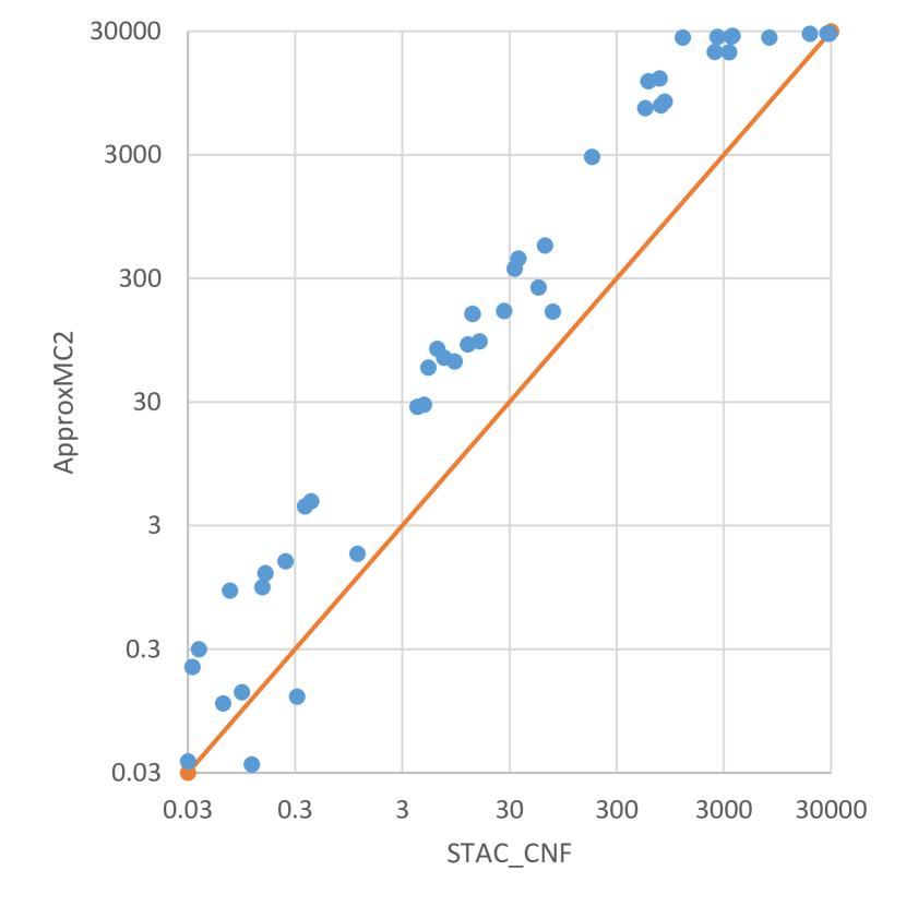
Figure 1: Performance comparison between STAC_CNF and ApproxMC2 with $\epsilon=0.8,\delta=0.2$ and 8 hours timeout

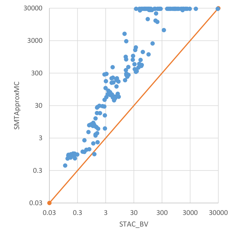
Figure 2: Performance comparison between STAC_BV and SMTApproxMC with $\epsilon=0.8,\delta=0.2$ and 8 hours timeout

We first conducted experiments with $\epsilon=0.8,\delta=0.2$ which are also used in evaluation in previous works [9, 6]. Figure 2 presents a comparison on performance between STAC_CNF and ApproxMC2. Each point represents an instance, whose $x$-coordinate and $y$-coordinate are the running times of STAC_CNF and ApproxMC2 on this instance, respectively. The figure is in logarithmic coordinates and demonstrates that STAC_CNF outperforms ApprxMC2 by about one order of magnitude. Figure 2 presents a similar comparison on performance between STAC_BV and SMTApproxMC, showing that STAC_BV outperforms SMTApproxMC by one or two order of magnitude. Furthermore, the advantage enlarges as the scale grows.

Table 4: Performance comparison between STAC_CNF and ApproxMC2 with different pairs of $(\epsilon,\delta)$ parameters

		blockmap				fs-01	5step	ran5	ran6	ran7
		05_01	05_02	10_01
$(0.8,0.3)$	Time Ratio	1.11	3.99	1.22		3.00	3.83	6.53	8.24	5.57
	#Calls Ratio	22.60	39.02	17.91		19.12	23.11	22.53	21.28	23.68
$(0.8,0.2)$	Time Ratio	1.84	6.16	2.44		2.80	6.05	9.61	15.41	7.37
	#Calls Ratio	26.70	34.68	25.16		33.46	27.24	33.35	38.22	30.94
$(0.8,0.1)$	Time Ratio	2.27	7.36	3.72		5.25	12.62	9.60	9.54	8.19
	#Calls Ratio	44.88	48.26	40.01		49.40	43.03	46.12	44.84	52.63
$(0.4,0.3)$	Time Ratio	0.75	1.37	0.42		3.00	5.04	1.97	2.31	2.74
	#Calls Ratio	17.75	36.20	14.69		16.40	27.63	21.07	27.34	21.63
$(0.4,0.2)$	Time Ratio	0.77	1.44	0.86		4.50	7.70	2.82	1.77	3.02
	#Calls Ratio	20.91	26.35	29.16		26.72	40.66	26.49	27.82	28.94
$(0.4,0.1)$	Time Ratio	1.08	2.57	1.29		4.90	7.09	3.84	3.43	3.11
	#Calls Ratio	37.16	46.28	39.40		31.99	39.36	41.02	35.88	34.11
$(0.2,0.3)$	Time Ratio	0.42	0.47	0.23		5.08	3.79	1.26	1.14	1.81
	#Calls Ratio	13.75	20.82	24.35		13.37	19.74	25.20	19.19	20.06
$(0.2,0.2)$	Time Ratio	0.57	0.92	0.26		8.42	3.37	2.07	1.50	2.45
	#Calls Ratio	21.80	29.62	25.60		21.83	21.59	25.88	22.72	22.98
$(0.2,0.1)$	Time Ratio	0.87	0.92	0.44		16.69	3.17	3.61	2.27	2.60
	#Calls Ratio	27.86	29.91	33.36		34.17	31.58	40.81	29.01	29.90

Table 4 presents more experimental results with $(\epsilon,\delta)$ parameters other than $(0.8,0.2)$. Nine pairs of parameters were experimented. “Time Ratio” represents the ratio of the running times of ApproxMC2 to STAC_CNF. “#Calls Ratio” represents the ratio of the number of SAT calls of ApproxMC2 to STAC_CNF. The results show that ApproxMC2 gains advantage as $\epsilon$ decreases and STAC_CNF gains advantage as $\delta$ decreases. On the whole, ApproxMC2 gains advantage when $\epsilon$ and $\delta$ both decrease. Note that the numbers of SAT calls represent the complexity of both algorithms. In Table 4, #Calls Ratio is more stable than Time Ratio among different pairs of parameters and also different instances. It indicates that the difficulty of NP-oracle is also an important factor of running time performance.

6.3 Performance Comparison with Bounding and Guarantee-less Counters

Since our approach is not a $(\epsilon,\delta)$-counter in theory, we also compared STAC_CNF with bounding counters (SampleCount [16], MBound [17]) and guarantee-less counters (ApproxCount [33], SampleTreeSearch [14]). Table 5 shows the experimental results.

Table 5: Performance comparison of STAC_CNF with existing bounding counters and guarantee-less counters

Instance	$n$	$\#F$	STAC_CNF			SampleCount			MBound			ApproxCount			SampleTreeSearch
		(if known)	($\epsilon=0.8,\delta=0.2$)			(99% confidence)			(99% confidence)
			Models	Time		L-bound	Time		L-bound	Time		Models	Time		Models	Time
blockmap_05_01	1411	640	$\approx 807$	1 s		$\geq 22$	116 s		$>64$	9 s		$=640$	7 s		$\approx 646$	71 s
blockmap_05_02	1738	$9.4\times 10^{6}$	$\approx 7.1\times 10^{6}$	16 s		$3.6\times 10^{4}$	5 m		$>2.1\times 10^{6}$	5 m		$=9.4\times 10^{6}$	13 s		$\approx 9.4\times 10^{6}$	114 s
blockmap_10_01	11328	$2.9\times 10^{6}$	$\approx 2.6\times 10^{6}$	96 s		—	$\geq$8 h		$>5.2\times 10^{5}$	9 m		—	$\geq$8 h		$\approx 3.0\times 10^{6}$	62 m
blockmap_15_01	33035	—	$\approx 2.0\times 10^{9}$	41 m		—	$\geq$8 h		—	$\geq$8 h		—	$\geq$8 h		—	$\geq$8 h
fs-01	32	768	$\approx 709$	0.1 s		$\geq 68$	0.2 s		$>64$	2 s		$\approx 925$	17 s		$\approx 769$	0.1 s
PLAN RECOGNITION
5step	177	$8.1\times 10^{4}$	$\approx 8.1\times 10^{4}$	0.2 s		$\geq 2.8\times 10^{3}$	4 s		$>8.2\times 10^{3}$	6 s		$=8.1\times 10^{4}$	18 s		$\approx 7.5\times 10^{4}$	1 s
tire-1	352	$7.3\times 10^{8}$	$\approx 9.8\times 10^{8}$	64 m		$\geq 7.0\times 10^{5}$	14 s		$>6.7\times 10^{7}$	8 h		$=7.3\times 10^{8}$	48 s		$\approx 7.6\times 10^{8}$	5 s
tire-3	577	$2.2\times 10^{11}$	—	$\geq$8 h		$\geq 1.3\times 10^{6}$	49 s		—	$\geq$8 h		$\approx 2.1\times 10^{11}$	63 s		$\approx 1.2\times 10^{11}$	5 s
LANGFORD PROBS.
lang12	576	$2.2\times 10^{5}$	$\approx 3.2\times 10^{5}$	80 m		$\geq 3.6\times 10^{3}$	3 m		$>1.6\times 10^{4}$	4 h		$\approx 0$	111 s		$\approx 1.9\times 10^{5}$	101 m
lang15	1024	—	—	$\geq$8 h		$\geq 4.7\times 10^{5}$	4 m		—	$\geq$8 h		$\approx 0$	122 s		—	$\geq$8 h
DQMR NETWORKS
or-100-20-6-UC-60	200	$2.8\times 10^{7}$	$\approx 3.4\times 10^{7}$	14 m		$\geq 1.1\times 10^{29}$	15 s		$>4.2\times 10^{6}$	6 m		$\approx 0$	17 s		$\approx 2.8\times 10^{7}$	0.8 s
or-50-10-10-UC-40	100	$3.1\times 10^{3}$	$\approx 3.2\times 10^{3}$	0.1 s		$\geq 2.7\times 10^{2}$	0.1 s		$>5.1\times 10^{2}$	4 s		$\approx 2.1\times 10^{16}$	68 s		$\approx 3.1\times 10^{3}$	0.5 s
or-50-20-10-UC-30	100	$6.8\times 10^{8}$	$\approx 7.4\times 10^{8}$	35 m		$\geq 6.0\times 10^{7}$	0.2 s		$>1.3\times 10^{8}$	3 h		$\approx 2.7\times 10^{16}$	62 s		$\approx 7.9\times 10^{8}$	0.7 s
or-60-10-10-UC-30	120	$6.8\times 10^{7}$	$\approx 6.2\times 10^{7}$	4 m		$\geq 1.0\times 10^{17}$	9 s		$>1.7\times 10^{7}$	38 m		$\approx 2.4\times 10^{19}$	83 s		$\approx 6.5\times 10^{7}$	1 s
or-60-5-2-UC-40	120	$2.1\times 10^{6}$	$\approx 1.9\times 10^{6}$	6 s		$\geq 1.0\times 10^{17}$	16 s		$>5.2\times 10^{5}$	199 s		$\approx 2.3\times 10^{19}$	89 s		$\approx 2.1\times 10^{6}$	0.9 s
or-70-10-6-UC-40	140	$1.2\times 10^{4}$	$\approx 7.2\times 10^{3}$	0.1 s		$\geq 1.0\times 10^{20}$	7 s		$>2.0\times 10^{3}$	4 s		$\approx 0$	165 s		$\approx 1.2\times 10^{4}$	0.5 s
or-70-5-2-UC-30	140	$1.7\times 10^{7}$	$\approx 4.7\times 10^{7}$	51 s		$\geq 1.0\times 10^{20}$	10 s		$>2.1\times 10^{6}$	11 m		$\approx 0$	165 s		$\approx 1.7\times 10^{7}$	0.8 s
RANDOM 3-CNF
ran6	30	$1.2\times 10^{6}$	$\approx 1.9\times 10^{6}$	0.6 s		$\geq 1.1\times 10^{5}$	0.2 s		$>1.3\times 10^{5}$	11 s		$\approx 8.3\times 10^{5}$	23 s		$\approx 1.3\times 10^{6}$	0.2 s
ran12	40	$3.5\times 10^{8}$	$\approx 4.2\times 10^{8}$	10 m		$\geq 3.1\times 10^{7}$	0.5 s		$>6.7\times 10^{7}$	15 m		$\approx 2.6\times 10^{8}$	23 s		$\approx 3.9\times 10^{8}$	0.3 s
ran27	50	$1.5\times 10^{8}$	$\approx 1.2\times 10^{8}$	8 m		$\geq 1.3\times 10^{7}$	18 s		$>1.7\times 10^{7}$	28 m		$\approx 5.5\times 10^{7}$	59 s		$\approx 1.1\times 10^{8}$	0.3 s
ran44	60	$1.1\times 10^{6}$	$\approx 1.9\times 10^{6}$	6 s		$\geq 9.5\times 10^{4}$	8 s		$>1.3\times 10^{5}$	52 s		$\approx 3.3\times 10^{5}$	139 s		$\approx 9.1\times 10^{5}$	0.5 s

For SampleCount, we used $\alpha=2$ and $t=3.5$ so that $\alpha t=7$, giving a correctness confidence of $1-2^{-7}=99\%$. The number of samples per variable setting, $z$, was chosen to be 20. Our results show that the lower-bound approximated by SampleCount is smaller than exact count $\#F$ by one or more orders of magnitude. We tried larger $z$, such as $z=100$ and $z=1000$, but still failed to obtain a lower-bound larger than $\#F/10$. Moreover, there are some wrong approximations on DQMR networks problems, e.g., or-100-20-6-UC-60 only has $2.8\times 10^{7}$ models but SampleCount returns a lower-bound $\geq 1.1\times 10^{29}$. SampleCount is more efficient on Langford problems and random 3-CNF problems, but weak on problems with a large number of variables, such as blockmap problems.

For MBound, we used $\alpha=1$ and $t=7$ so that $\alpha t=7$, also giving a correctness confidence of $1-2^{-7}=99\%$. MBound also employs a family of XOR hashing function which is similar to the function used by our approach. The size of XOR constraints $k$ should be no more than half of the number of variables $n$, i.e., $k\leq n/2$. We found that XOR constraints start to fail as $k<<n/2$. So in our experiments, $k$ was chosen to be close to $n/2$. Since MBound can only check the bound and may return failure as the bound too close to the exact count, we implemented a binary search to find the best lower-bound verified by MBound. The results in Table 5 are the best lower-bounds and the running times of the whole binary search procedure. Though the lower-bounds are better than SampleCount, they are still around $\#F/10$. Similar to our approach, the running times of MBound are also quite relevant to the size of $\#F$.

For ApproxCount, we manually increased the value of “cutoff” as ApproxCount required. Note that ApproxCount calls exact model counter Cachet [27] and Relsat [20] after formula simplifications, so it sometimes returns the exact counts, such as blockmap_05_01, blockmap_05_02, 5step and tire-1. On Langford problems and DQMR networks problems, wrong approximations were provided. On other instances, the results show that STAC_CNF usually outperforms ApproxCount.

For SampleTreeSearch, we used its default setting about the number of samples, which is a constant. The results show that it is very efficient and provides good approximations. Our approach only outperforms SampleTreeSearch on blockmap problems which consist of a large number of variables. However, there is a lack of analysis on the accuracy of the approximation of SampleTreeSearch, i.e., no explicit relation between the number of samples and the accuracy.

7 Conclusion

In this paper, we propose a new hashing-based approximate algorithm with dynamic stopping criterion. Our approach has two key strengths: it requires only one satisfiability query for each cut, and it terminates once meeting the theoretical guarantee of accuracy. We implemented prototype tools for propositional logic formulas and SMT(BV) formulas. Extensive experiments demonstrate that our approach is efficient and promising. Despite that we are unable to prove the correctness of Equation (1), the experimental results fit it quite well. This phenomenon might be caused by some hidden properties of the hash functions. To fully understand these functions and their correlation with the model count of the hashed formula might be an interesting problem to the community. In addition, extending the idea in this paper to count solutions of other formulas is also a direction of future research.

References

- [1] M. Bellare, O. Goldreich, and E. Petrank. Uniform generation of NP-witnesses using an NP-oracle. Inf. Comput., 163(2):510–526, 2000.
- [2] V. Belle, G. V. Broeck, and A. Passerini. Hashing-based approximate probabilistic inference in hybrid domains. In Proc. of UAI, pages 141–150, 2015.
- [3] L. D. Brown, T. T. Cai, and A. Dasgupta. Interval estimation for a binomial proportion. Statistical Science, 16(2):101–133, 2001.
- [4] R. Brummayer and A. Biere. Boolector: An efficient SMT solver for bit-vectors and arrays. In Proc. of TACAS, pages 174–177, 2009.
- [5] S. Chakraborty, D. J. Fremont, K. S. Meel, S. A. Seshia, and M. Y. Vardi. Distribution-aware sampling and weighted model counting for SAT. In Proc of AAAI, pages 1722–1730, 2014.
- [6] S. Chakraborty, K. S. Meel, R. Mistry, and M. Y. Vardi. Approximate probabilistic inference via word-level counting. In Proc. of AAAI, pages 3218–3224, 2016.
- [7] S. Chakraborty, K. S. Meel, and M. Y. Vardi. A scalable and nearly uniform generator of SAT witnesses. In Proc. of CAV, pages 608–623, 2013.
- [8] S. Chakraborty, K. S. Meel, and M. Y. Vardi. A scalable approximate model counter. In Proc. of CP, pages 200–216, 2013.
- [9] S. Chakraborty, K. S. Meel, and M. Y. Vardi. Algorithmic improvements in approximate counting for probabilistic inference: From linear to logarithmic SAT calls. In Proc. of IJCAI, pages 3569–3576, 2016.
- [10] M. Chavira and A. Darwiche. On probabilistic inference by weighted model counting. Artif. Intell., 172(6-7):772–799, 2008.
- [11] D. Chistikov, R. Dimitrova, and R. Majumdar. Approximate counting in SMT and value estimation for probabilistic programs. In Proc. of TACAS, pages 320–334, 2015.
- [12] C. Domshlak and J. Hoffmann. Probabilistic planning via heuristic forward search and weighted model counting. J. Artif. Intell. Res. (JAIR), 30:565–620, 2007.
- [13] S. Ermon, C. P. Gomes, A. Sabharwal, and B. Selman. Embed and project: Discrete sampling with universal hashing. In Advances in Neural Information Processing Systems 26, pages 2085–2093, 2013.
- [14] S. Ermon, C. P. Gomes, and B. Selman. Uniform solution sampling using a constraint solver as an oracle. In Proc. UAI, pages 255–264, 2012.
- [15] J. Geldenhuys, M. B. Dwyer, and W. Visser. Probabilistic symbolic execution. In Proc. of ISSTA, pages 166–176, 2012.
- [16] C. P. Gomes, J. Hoffmann, A. Sabharwal, and B. Selman. From sampling to model counting. In Proc. of IJCAI, pages 2293–2299, 2007.
- [17] C. P. Gomes, A. Sabharwal, and B. Selman. Model counting: A new strategy for obtaining good bounds. In Proc. of AAAI, pages 54–61, 2006.
- [18] C. P. Gomes, A. Sabharwal, and B. Selman. Near-uniform sampling of combinatorial spaces using XOR constraints. In Advances in Neural Information Processing Systems 19, pages 481–488, 2006.
- [19] A. Ivrii, S. Malik, K. S. Meel, and M. Y. Vardi. On computing minimal independent support and its applications to sampling and counting. Constraints, 21(1):41–58, 2016.
- [20] R. J. Bayardo Jr. and R. Schrag. Using CSP look-back techniques to solve real-world SAT instances. In Proc. of AAAI, pages 203–208, 1997.
- [21] R. M. Karp, M. Luby, and N. Madras. Monte-carlo approximation algorithms for enumeration problems. J. Algorithms, 10(3):429–448, 1989.
- [22] L. Kroc, A. Sabharwal, and B. Selman. Leveraging belief propagation, backtrack search, and statistics for model counting. Annals of OR, 184(1):209–231, 2011.
- [23] S. Liu and J. Zhang. Program analysis: from qualitative analysis to quantitative analysis. In Proc. of ICSE, pages 956–959, 2011.
- [24] K. S. Meel, M. Y. Vardi, S. Chakraborty, D. J. Fremont, S. A. Seshia, D. Fried, A. Ivrii, and S. Malik. Constrained sampling and counting: Universal hashing meets SAT solving. In Proceedings of Workshop on Beyond NP(BNP), 2016.
- [25] D. Roth. On the hardness of approximate reasoning. Artif. Intell., 82(1-2):273–302, 1996.
- [26] T. Sang, P. Beame, and H. A. Kautz. Performing bayesian inference by weighted model counting. In Proc. of AAAI, pages 475–482, 2005.
- [27] Tian Sang, Fahiem Bacchus, Paul Beame, Henry A. Kautz, and Toniann Pitassi. Combining component caching and clause learning for effective model counting. In Proc. of SAT, 2004.
- [28] M. Sipser. A complexity theoretic approach to randomness. In Proc. of the 15th Annual ACM Symposium on Theory of Computing, pages 330–335, 1983.
- [29] M. Soos, K. Nohl, and C. Castelluccia. Extending SAT solvers to cryptographic problems. In Proc. of SAT, pages 244–257, 2009.
- [30] L. J. Stockmeyer. The complexity of approximate counting (preliminary version). In Proc. of the 15th Annual ACM Symposium on Theory of Computing, pages 118–126, 1983.
- [31] L. G. Valiant. The complexity of enumeration and reliability problems. SIAM J. Comput., 8(3):410–421, 1979.
- [32] S. Wallis. Binomial confidence intervals and contingency tests: Mathematical fundamentals and the evaluation of alternative methods. Journal of Quantitative Linguistics, 20(3):178–208, 2013.
- [33] W. Wei and B. Selman. A new approach to model counting. In Proc. of SAT, pages 324–339, 2005.
- [34] E. B. Wilson. Probable inference, the law of succession and statistical inference. Journal of the American Statistical Association, 22(158):209–212, 1927.