Active plasmon injection scheme for subdiffraction imaging with imperfect negative index flat lens

Abstract

We present an active physical implementation of the recently introduced plasmon injection loss compensation scheme for Pendry’s non-ideal negative index flat lens in the presence of realistic material losses and signal-dependent noise. In this active implementation, we propose to use a physically convolved external auxiliary source for signal amplification and suppression of the noise in the imaging system. In comparison with the previous passive implementations of the plasmon injection scheme for sub-diffraction limited imaging, where an inverse filter post-processing is used, the active implementation proposed here allows for deeper subwavelength imaging far beyond the passive post-processing scheme by extending the loss compensation to even higher spatial frequencies.

I Introduction

Controlling the interaction of photons and electrons at the sub-wavelength electromagnetic regime has led to a wide variety of novel optical materials and applications in the territory of metamaterials and plasmonics relevant to computing, communications, defense, health, sensing, imaging, energy, and other technologies Fang534 ; taubner2006near ; zhang2008superlenses ; liu2007far ; rho2010spherical ; lu2012hyperlenses ; sun2015experimental ; lee2007development ; valentine2008three ; landy2008perfect ; temnov2012ultrafast ; aslam2012negative ; sadatgol2016enhanced ; choi2011terahertz ; chen2012extremely ; zhang2015extremely ; schurig2006metamaterial ; gwamuri2013advances ; rockstuhl2008absorption ; vora2014exchanging ; vora2014multi ; bulu2005compact ; odabasi2013electrically ; guney2009negative ; smolyaninov2010metric ; tame2013quantum ; al2015quantum ; asano2015distillation ; jha2015metasurface ; sperling2008biological ; huang2006cancer ; lal2008nanoshell ; guo2010multifunctional ; doi:10.1021/nl304208s ; blankschien2012light ; chen2010enhanced ; sherlock2011photothermally ; ahmadivand2015enhancement . The prospect of circumventing Rayleigh’s diffraction limit, thereby allowing super-resolution imaging has regained tremendous ground since Pendry theorised that a slab of negative (refractive) index material (NIM) can amplify and focus evanescent fields which contain information about the sub-wavelength features of an object Pendry . A recent review of super-resolution imaging in the context of metamaterials is given in adams2016review .

However, a perfect NIM does not exist in nature and although recent developments in metamaterials have empowered their realization, a fundamental limitation exists. The presence of material losses in the near infrared and visible region is significant PhysRevLett.95.137404 ; RN4 ; Dolling892 . This compromises the performance of the theoretical perfect lens Webb1 ; Yang:05 since a significant portion of evanescent fields is below the noise floor of the detector and are indiscernible. Therefore, new efforts were directed towards the compensation of losses in metamaterials Nezhad:04 ; Popov:06 ; PhysRevB.80.125129 . Amongst the schemes that were developed, gain media to compensate intrinsic losses gained popularity Anantha ; refId0 . However, Stockman PhysRevLett.98.177404 demonstrated that the use of gain media involved a fundamental limitation. Using the Kramers-Kronig relations, they developed a rule based on causality which makes loss compensation with gain media difficult to realize.

Recently, a new compensation scheme, called plasmon injection or $\Pi$ scheme PI , was proposed. The $\Pi$ scheme was conceptualized with surface plasmon driven NIMs Aslam and achieves loss compensation by coherently superimposing externally injected surface plasmon polaritons (SPPs) with local SPPs. Therefore, absorption losses in the NIM could be removed without a gain medium or non-linear effects. Although the $\Pi$ scheme was originally envisioned for plasmonic metamaterials PI ; guney2011surface ; aslam2012dual , the idea is general and can be applied to any type of optical modes. In Wyatt Adams, et. al used a post processing technique equivalent to this method. They demonstrated that the process can indeed be used to amplify the attenuated Fourier components and thereby accurately resolve an object with sub-wavelength features.

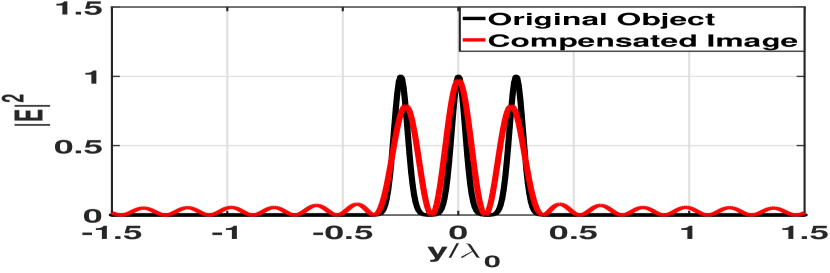
Figure 1: Electric field magnitude squared $[Vm^{-1}]^{2}$ distribution in the object and image planes for an object with features separated by $\lambda_{o}/4$ with $\lambda_{o}=1\mu m$. The compensated image is reasonably well resolved with the equivalent inverse filter post-processing technique.

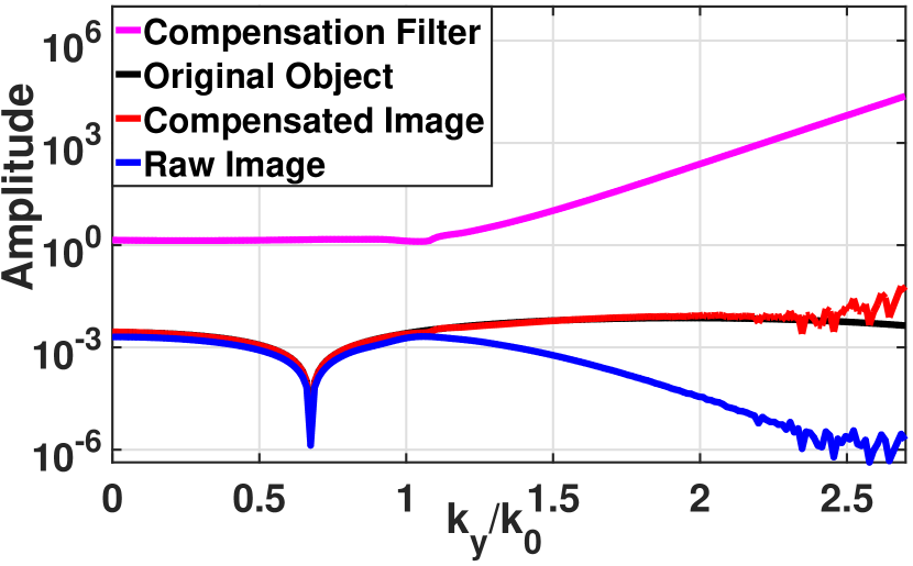
Figure 2: Fourier spectra $[Vm^{-1}]$ of the three Gaussians and the compensated image in figure 1, and the raw image obtained without loss compensation. The compensation filter is the inverse of the transfer function. The compensated image spectrum is obtained simply by multiplying the raw image spectrum with the compensation filter. Notice that the noise can be seen for high spatial frequencies which is amplified by the compensation.

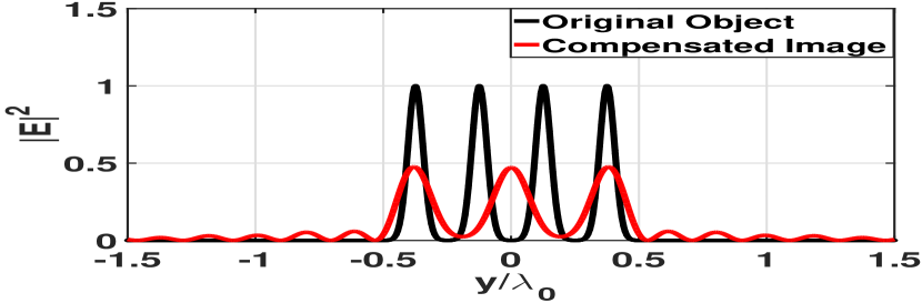
Figure 3: Electric field magnitude squared $[Vm^{-1}]^{2}$ for the four Gaussians, in the object and image planes, separated by $\lambda_{o}/4$ with $\lambda_{o}=1\mu m$. The compensated image is very poorly resolved with one of the Gaussians missing.

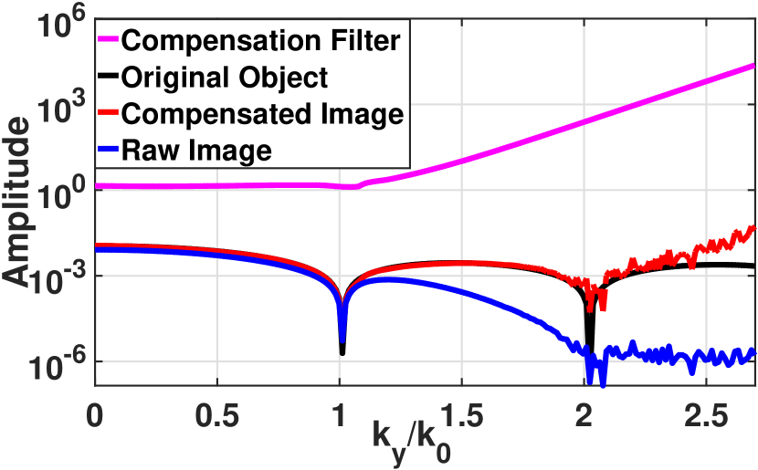
Figure 4: Fourier spectra $[Vm^{-1}]$ of the four Gaussians and the compensated image in figure 3, and the raw image along with the compensation filter. Notice that the feature at $\frac{k_{y}}{k_{o}}=2$ is not discernable under the noise and cannot be recovered well with the compensation.

Although this form of passive inverse filter provides compensation for absorption losses, it is also prone to noise amplification Wyatt . This is illustrated in figure 1 which shows an object with three Gaussian features separated by $\lambda_{o}/4$, where $\lambda_{o}$ is the free space wavelength. Noise is prominent in the Fourier spectra beyond $\frac{k_{y}}{k_{o}}=2.5$ as seen in figure 2. However, the compensated image is still reasonably well resolved. Consider now the object shown in figure 3, which has four Gaussians separated by $\lambda_{o}/4$. The Fourier spectra of the raw image, shown in figure 4, demonstrates how the feature at $\frac{k_{y}}{k_{o}}=2$ is not distinguishable under the noise. The final compensated image, when subject to the same compensation scheme, is poorly resolved. We define a feature as any spatial Fourier component that has substantial contribution to the shape of the object. It is clear that the Fourier components beyond $\frac{k_{y}}{k_{o}}=2$ have a significant contribution to the four Gaussians and must be recovered from the image spectrum in order to accurately resolve the object. Therefore, noise presents a limitation which must be overcome to make the $\Pi$ scheme versatile.

In the present work, we demonstrate how the $\Pi$ scheme can be significantly improved with the use of a physical auxiliary source to recover high spatial frequency features that are buried under the noise. We show that by using a convolved auxiliary source we can amplify the object spectrum in the frequency domain. The amplification makes the Fourier components that are buried in the noise distinguishable. This allows for the recovery of the previously inaccessible object features by adjusting the amount of compensation from the $\Pi$ scheme.

The technique presented in this paper is based on the same negative index flat lens (NIFL) as in Wyatt . We use the words ”passive” and ”active” to distinguish between the compensation schemes applied in Wyatt and in this work, respectively. Therefore, the inverse filter post processing used in Wyatt and figures 1-4 to emulate the physical compensation of losses can be called passive $\Pi$ scheme, since no external physical auxiliary is actively involved as opposed to the active $\Pi$ scheme here, where the direct physical implementation using an external auxiliary source as originally envisioned in PI is sought. The active compensation scheme allows us to control noise amplification and hence extend the applicability of the $\Pi$ scheme to higher spatial frequencies.

II Theory

We define the optical properties of the NIFL with the relative permittivity and permeability expressed as $\epsilon_{r}=\epsilon^{{}^{\prime}}+i\epsilon^{{}^{\prime\prime}}$ and $\mu_{r}=\mu^{{}^{\prime}}+i\mu^{{}^{\prime\prime}}$, where $\epsilon^{{}^{\prime}}=-1$ and $\mu^{{}^{\prime}}=-1$. COMSOL Multiphysics, the finite element method based software package that we use here, assumes $exp(j\omega t)$ time dependence. Therefore, the imaginary parts of $\epsilon_{r}$ and $\mu_{r}$ are negative for passive media. In this paper we have used $0.1$ as the imaginary parts of both $\epsilon_{r}$ and $\mu_{r}$ which is a reasonable value given currently fabricated metamaterial structures RN1 ; Garc ; Verhagen . The geometry used to numerically simulate the NIFL in COMSOL is given in figure 5. The first step is characterizing the NIFL with a transfer function. For a detailed discussion on the geometry setup and transfer function calculations, the reader is referred to Wyatt . Here, we present a brief mathematical description of the compensation scheme.

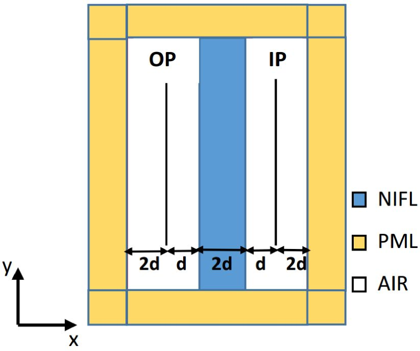
Figure 5: The geometry built in COMSOL to perform numerical simulations (not to scale). OP and IP are the object and image planes, respectively. Electric field is polarized along the z-axis (pointing out of plane). The object is defined as an electric field distribution $[E_{z}(y)]$ on the object plane. The operating wavelength is $\lambda_{o}=1\mu m$ and $2d=0.5\mu m$. Blue, white, and orange regions are the NIFL, air, and perfectly matched layer (PML), respectively.

The spatial Fourier transforms of the electric fields in the object and image planes are related by the passive transfer function, $T_{P}(k_{y})$ of the imaging system, which can be calculated with COMSOL. This is expressed mathematically as

$$I(k_{y})=T_{P}(k_{y})O(k_{y}).$$ (1)

Here $O(k_{y})=\mathcal{F}\{O(y)\}$ and $I(k_{y})=\mathcal{F}\{I(y)\}$, where $O(y)$ and $I(y)$ are the spatial distribution of the electric fields in the object and image planes, respectively, and $\mathcal{F}$ is the Fourier transform operator. According to Wyatt the passive compensation is defined by the inverse of the transfer function. Hence, the loss compensation is achieved by multiplying the raw image spectrum in Eq. 1 with the inverse of the transfer function given by

$$C_{P}(k_{y})=\bigg{[}T_{P}(k_{y})\bigg{]}^{-1}.$$ (2)

For ”active” compensation we first define a mathematical expression given by

$$A(k_{y})=1+P(k_{y}),$$ (3)

$$P(k_{y})=P_{o}exp\bigg{[}-\frac{(\frac{k_{y}}{k_{o}}-k_{c})^{2}}{2\sigma^{2}}\bigg{]},$$ (4)

where $P_{o}$ is a constant. $k_{c}$ controls the center frequency of the Gaussian, $k_{o}=\frac{2\pi}{\lambda}$ is the free space wave number and $\sigma$ controls the full width at half maximum (FWHM) of the Gaussian. We convolve $A(y)=\mathcal{F}^{-1}\{A(k_{y})\}$ with the object $O(y)$ in the spatial domain and denote the new object by $O^{{}^{\prime}}(y)$. This is expressed as

$$O^{{}^{\prime}}(y)=\int\limits^{\infty}_{-\infty}O(y)A(y-\alpha)d\alpha.$$ (5)

We shall refer to this convolved object as the total object. Since convolution in the spatial domain is equivalent to multiplication in the spatial frequency domain, the Fourier spectrum of the total object $O^{{}^{\prime}}(k_{y})=\mathcal{F}\{O^{{}^{\prime}}(y)\}$, is related to the original object by

$$O^{{}^{\prime}}(k_{y})=O(k_{y})+O(k_{y})P(k_{y}).$$ (6)

The second term on the RHS will be referred to as the ”auxiliary source,” where $P_{o}$ in Eq. 4 defines its amplitude at the center frequency $k_{c}$ . Note that this term, which is a convolution of $O(y)$ with $P(y)=\mathcal{F}^{-1}\{P(k_{y})\}$, represents amplification in the spatial frequency domain provided that $P(k_{y})>1$. Even though the auxiliary source is object dependent, as we will discuss later, the external field to generate auxiliary source does not require prior knowledge about the object. Now, the Fourier transform of the fields in the object and image planes are related to each other by the transfer function of the NIFL as defined by Eq. 1. Therefore, in response to the total object, the new field distribution in the image plane, expressed as $I^{{}^{\prime}}(y)=\mathcal{F}^{-1}\{I^{{}^{\prime}}(k_{y})\}$, is transformed as

$$I^{{}^{\prime}}(k_{y})=T_{P}(k_{y})O^{{}^{\prime}}(k_{y}),$$ (7)

where we can plug in the value of $O^{{}^{\prime}}(k_{y})$ from Eq. 6 to obtain the convolved image

$$I^{{}^{\prime}}(k_{y})=T_{P}(k_{y})O(k_{y})+T_{P}(k_{y})O(k_{y})P(k_{y}).$$ (8)

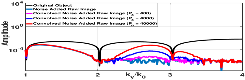
Figure 6: Fourier spectra [$Vm^{-1}$] of an arbitrary object illustrating how the auxiliary amplitude can be tuned from the object plane to raise the image spectrum above the noise floor by controlling the amplification. $P(k_{y})$ is centered at $k_{c}=\frac{k_{y}}{k_{o}}=3$ with $\sigma=0.13.$

The second term on the RHS of Eq. 8 is a measure of the residual amplification which managed to propagate to the image plane. Therefore, by controlling $P_{o}$, from the object plane, we can tune the necessary amplification of high spatial frequency features to raise the desired frequency spectrum above the noise floor in the image plane. This process is illustrated in figure 6 for different auxiliary amplitudes.

The new ”active” loss compensation scheme must consider the extra power that is now available in the image spectrum. We distinguish the compensation scheme from Eq. 2 with the subscript ”A”. We start by defining the active transfer function of the NIFL as

$$T_{A}(k_{y})=\frac{I^{{}^{\prime}}(k_{y})}{O(k_{y})}.$$ (9)

The numerator of Eq. 9 is the image of the total object which is given by Eq. 8. This transfer function is called ”active” because it considers the auxiliary to be a part of the imaging system. Plugging in the value of $I^{{}^{\prime}}(k_{y})$ from Eq. 8 into Eq. 9 we obtain the following expression for the active transfer function,

$$T_{A}(k_{y})=T_{P}(k_{y})+T_{P}(k_{y})P(k_{y}).$$ (10)

The active compensation filter is simply defined as the inverse of the active transfer function and is expressed mathematically by

$$C_{A}(k_{y})=\bigg{[}T_{P}(k_{y})+T_{P}(k_{y})P(k_{y})\bigg{]}^{-1}.$$ (11)

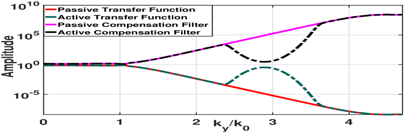
Figure 7: Comparisons of the passive transfer function $T_{P}(k_{y})$ and compensation filter $C_{P}(k_{y})$ with the active transfer function $T_{A}(k_{y})$ and compensation filter $C_{A}(k_{y})$. $P(k_{y})$ incorporated into the active compensation filter is centered at $k_{c}=\frac{k_{y}}{k_{o}}=3$ with $\sigma=0.13$.

Figure 7 illustrates the active and passive transfer functions and the corresponding loss compensation schemes. The amount of active compensation drops within $2.5<\frac{k_{y}}{k_{o}}<3$. This indicates that in this region the auxiliary source is expected to provide compensation to the image. Therefore, the greater the auxiliary power, the lower is the required compensation through inverse filter within that region of spatial frequencies. It is interesting to note at this point the similarity of the active transfer functions in figure 7 and those in Chen:16 . In the latter, however, highly stringent conditions are imposed on the negative index lens to obtain such a transfer function.

III Noise Characterization

The active compensation scheme will be applied to an NIFL imaging system affected by noise where the noise process is a circular Gaussian random variable. Although there are many different sources of noise, they can be broadly classified into, ”signal-dependent” (SD) and ”signal-independent” (SI). The random nature of noise manifests itself in the form of an uncertainty in the level of the desired signal. This uncertainty is quantified by the standard deviation $\sigma_{n}$. The actual distortion can be thought of as a random selection from an infinite set of values and the selection process obeys a probability distribution function. The standard deviation describes the range of values which have the greatest likelihood of being selected. When the underlying signal is distorted by multiple independent sources of noise, each characterized by Gaussian distributions, then the variance $(\sigma_{n}^{2})$ of the total noise is the sum of the variances of individual noise sources Fiete .

SD noise, as the name implies, is characterized by a $\sigma_{n}$ that is intricately related to spatial (or temporal) variations in the incoming signal intensity. The magnitude of the signal distortion therefore also increases with the signal strength. Sources of SD noise in an imaging system can be present on the detector side or the transmission medium. For example, the statistical nature of photons manifests itself as noise which has Poissonian statistics. In radiographic detection equipment, such sources of noise are called quantum mottle or quantum noise 0031-9155-48-23-006 ; MP:MP5126 . Another source of SD noise originates from roughness of the transmission media, which in sub-wavelength imaging systems can be for example, surface roughness of the NIFL. One can think of surface irregularities as electromagnetic scatterers which radiate in different directions, distorting the propagating wave. Previous experiments on the impact of surface roughness Guo2014 ; Wang:11 ; Liu_Hong showed that increasing material losses in the NIFL improved the image resolution of the perfect lens for relatively large surface roughness. Although this may seem counter-intuitive, it can be explained if roughness is modelled as a source of scattering. Adding material loss is equivalent to lowering the power transmission of the lens. This lowers the magnitude of the excitation field responsible for scattering effects and in turn reduces the magnitude of the scattered field. If material losses are kept constant, the scattering process will be proportional to the intensity of illumination provided to the object. Therefore, such kind of noise is amplified as the illumination intensity is increased. On the other hand, the SI noise is quantified by a standard deviation which is not a function of the incoming signal. Therefore, the random nature of the noise will be visible only when the incoming signal amplitude is comparable to the distortions due to the SI noise. A good example of this is ”dark noise”, which affects a CCD sensor even in the absence of illumination holst1998ccd .

A well known model Walkup used to describe the spatial distribution of a signal that has been distorted with both SD and SI sources of noise is

$$r(y)=s(y)+f(s(y))N_{1}(y)+N_{2}(y),$$ (12)

where $s(y)$ is the noiseless or ideal signal and $r(y)$ is the noisy version. $N_{1}(y)$ and $N_{2}(y)$ are two statistically independent random noise processes with zero mean and Gaussian probabilities with standard deviations $\sigma_{n1}$ and $\sigma_{n2}$, respectively. The noise processes $N_{1}(y)$ and $N_{2}(y)$ are signal independent. The signal dependent nature of noise is modelled by modulating $N_{1}(y)$ using the function $f(s(y))$. Generally, $f(s(y))$ is a non-linear function of the ideal signal itself which is chosen based on the system which Eq. 12 is attempting to describe. For example, $f(s(y))$ is usually considered to be the photographic density which is unitless when modelling signal-dependent film grain noise. Therefore, $f(s(y))N_{1}(y)$ represents the effective signal dependent noise term. We can re-write the expression in Eq. 12 as

$$r(y)=s(y)+N_{SD}(y)+N_{SI}(y),$$ (13)

where the standard deviation of $N_{SD}(y)$ is $f(s(y))\sigma_{n1}$ and the subscripts SD, SI distinguish between the sources of noise. The noise model of Eq. 12, referred to as the signal modulated noise model, is used for signal estimation purposes with the Wiener filter. A detailed discussion on this can be found in Heine:06 ; Kasturi:83 ; Froehlich:81 ; Walkup . However, we will use Eq. 13 in this paper for mathematical convenience to analyse the relative contributions of SD and SI noise.

In the NIFL imaging system which we consider, the ideal signal $s(y)$ will be the electric field distribution on the image plane, that is $I(y)$ and $I^{{}^{\prime}}(y)$ for passive and active schemes, respectively. In Chen:16 , Chen, et. al adopted a $60dB$ signal to noise ratio (SNR) in their negative index lens considering an experimental imaging system detector Akiba:10 . This corresponds to a SD standard deviation of $10^{-3}I(y)$. In this work, we adopt the same standard for the SD noise. Additionally, we assume a SI noise process in the imaging system by adopting a spatially invariant standard deviation of $10^{-3}[V/m]$. This means that even in the absence of illumination, there is a constant background noise of the order of $1\ mV/m$ in the detector. Although the value of the SI noise is chosen arbitrarily, this does not limit the results discussed in this paper, since the SI noise can be easily suppressed by additional auxiliary power.

By taking into consideration the SNR standard used by Chen, et. al Chen:16 and the mathematical form of Eq. 13 we can frame the equations for the noisy images as

$$I_{N}(y)=I(y)+N_{SD}(y)+N_{SI}(y)$$ (14)

and

$$I^{{}^{\prime}}_{N}(y)=I^{{}^{\prime}}(y)+N^{{}^{\prime}}_{SD}(y)+N^{{}^{\prime}}_{SI}(y)$$ (15)

corresponding to the ideal images described by Eqs. 1 and 8, respectively. The subscript N indicates the noisy image. The standard deviations of the noise processes are

$$\sigma_{n(SD)}=10^{-3}I(y),$$ (16)

$$\sigma^{{}^{\prime}}_{n(SD)}=10^{-3}I^{{}^{\prime}}(y)$$ (17)

and

$$\sigma_{n(SI)}=\sigma^{{}^{\prime}}_{n(SI)}=10^{-3}\ V/m.$$ (18)

Eqs. 16 - 18 fully describe the random variables that are used to construct the SI and SD noise terms in Eqs. 14 and 15.

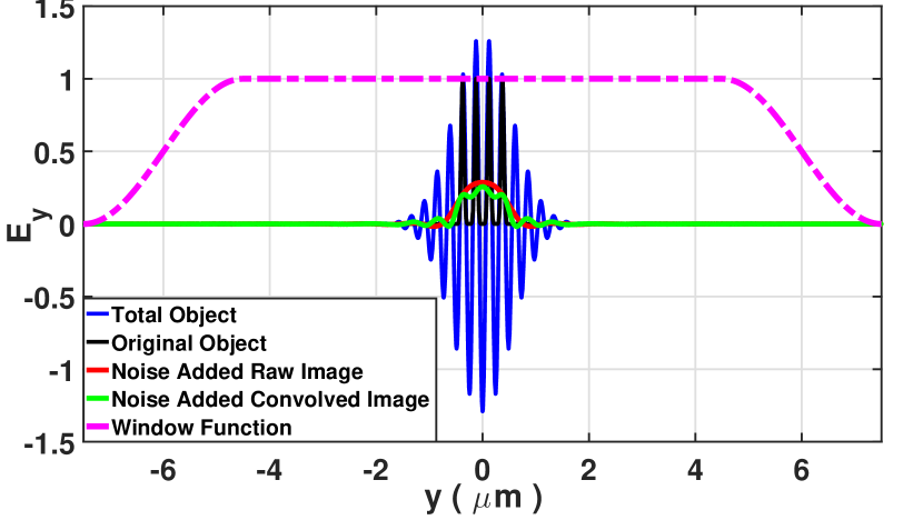
Figure 8: Electric field [$Vm^{-1}$] distributions in the object and image planes. The fields on the image planes are multiplied by the window function to reduce the errors in the Fourier transform. The total object has been scaled down by $\approx 10^{4}$.

IV Results

Having described how both SD and SI noise are added to the system, the next step is to evaluate the performance of active-compensation and compare with the passive version. We will attempt to image the previously exemplified object comprising four Gaussian features, separated by $\frac{\lambda_{o}}{4}$ with $\lambda_{o}=1\mu m$ and compare the results of passive and active compensation. Note that due to the finite extent of the image plane, it is necessary to multiply the electric fields with a window function to ensure that the field drops to zero where the image plane is abruptly terminated. Otherwise, errors are introduced in the Fourier transform calculations. Windowing the field distribution simply reduces these sources of error, which will be then visible only in the higher spatial frequencies. Since these errors are very small compared with the amplitude of the SD and SI sources of noise, they do not have a significant impact on the calculations. Increasing the length of the image plane along the y-axis can also reduce these errors, but because of computational constraints this may not be desirable.

Figure 8 shows the spatial electric field distributions on the object and image planes. Noise was artificially added to the fields on the image plane that were calculated with COMSOL. The resultant noisy images are indicated by the red and green lines in the figure. The Tukey (tapered cosine) window function was applied to the image plane only. The Fourier transforms of the images, with and without added noise are shown in figure 9. The black line, which corresponds to $I_{N}(k_{y})$ in Eq. 14, shows how the added noise has clearly affected the raw image spectrum beyond $\frac{k_{y}}{k_{o}}=2$, where all of the object features are now completely buried under the noise and indiscernible. However, the blue line, which corresponds to $I^{{}^{\prime}}_{N}(k_{y})$ in Eq. 15, shows how these features can be recovered with the convolved auxiliary.

We propose the following iterative process to apply the auxiliary source. We then use active compensation filter to reconstruct the image spectrum.

1. Select an arbitrary $k_{c}$ in the region where the noise has substantially degraded the spectrum. Choose a guess auxiliary amplitude by selecting $P_{0}$.

2. Convolve the object with $A(y)$ to obtain the total object.

3. Measure the electric fields on the image plane corresponding to the total object.

4. Re-scale $P_{0}$ for the selected $k_{c}$ if necessary, to make sure that adequate amplification is available in the image plane and noise is not visible in the Fourier spectrum.

5. Select another $k_{c}$ on the noise floor and ensure that there is sufficient overlap between the adjacent auxiliaries.

6. Repeat the processes in $1-5$ by superimposing those multiple auxiliaries until the transfer function of the imaging system is reasonably accurate. We were restricted by the inaccuracy of the simulated passive transfer function $T_{P}(k_{y})$ beyond $\frac{k_{y}}{k_{o}}=4.7$ which prevented us from going beyond.

Note that in the above steps the selection of $P_{o}$ does not require prior knowledge about the object. The blue and green lines of figure 9 show the total images with and without added noise, respectively. They include four auxiliary sources with the center frequencies $k_{c}=k_{y}/k_{o}=2.8,\ 3.1,\ 3.6,\ 4.2$ and $P_{o}=3000,\ 10000,\ 4\times 10^{5},\ 10^{6}$, respectively, with the same $\sigma=0.35$. The final $A(y)$ was then convolved with the object and the resulting total field distribution on the object plane is shown by the blue line in figure 8.

Active compensation filter, defined by Eq. 11 and illustrated in figure 10, is then multiplied in the spatial frequency domain by the total image spectrum with the added noise. The resulting compensated spectrum is the red line of figure 10. The noise, which was visible in the total image spectrum beyond $\frac{k_{y}}{k_{o}}=4.5$, is also amplified in this reconstruction process. However, in the regions where the auxiliary source is sufficiently strong, suppression of noise amplification is evident. The reconstructed spectrum perfectly coincides with the original object shown by the black curve in figure 10. The light blue line corresponds to the passively compensated image obtained by multiplying Eq. 2 (i.e., dark blue line in figure 10) with the noise added raw image (i.e., black line in figure 9). The advantage of the active compensation over its passive counterpart is therefore clearly evident from the reconstructed Fourier spectrum. After the loss compensation process, the spectrum is truncated at $\frac{k_{y}}{k_{o}}=4.7$ because the simulated transfer function loses accuracy.

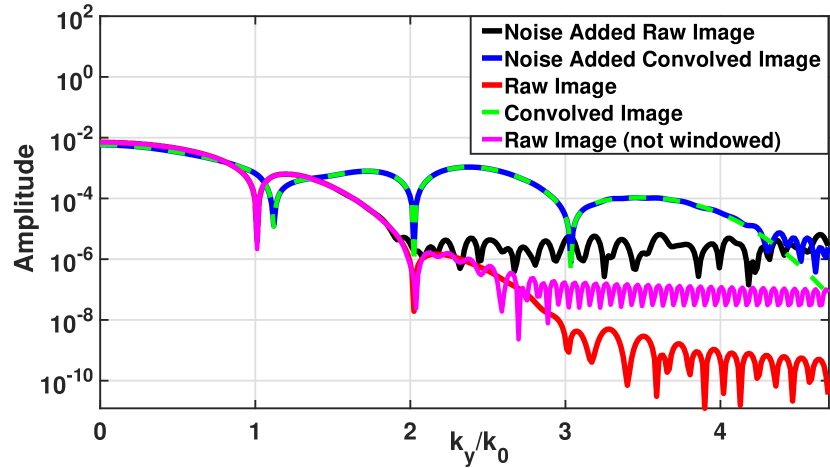
Figure 9: Amplitude of the Fourier transforms [$Vm^{-1}$] on a log scale. Red and green lines are the image spectra $I(k_{y})$ and $I^{{}^{\prime}}(k_{y})$ with no added noise, respectively. The blue line shows the image of the total object with added noise, $I^{{}^{\prime}}_{N}(k_{y})$. Noise is visible at $\frac{k_{y}}{k_{o}}\ >\ 4.5$ due to the inadequate amplification. The apparent noise in the pink line are due to the numerical errors introduced by the Fourier transform and shifts to higher $\frac{k_{y}}{k_{o}}$ values after applying the Tukey window as seen in the red line.

Figure 7 shows that the passive transfer function starts to flatten beyond $\frac{k_{y}}{k_{o}}=4.5$, even though the analytical transfer function monotonically decreases (see figure 3 in Chen:16 ), inaccurate simulated transfer function $T_{P}(k_{y})$ indicates that it is no longer possible to perform the required compensation accurately (see Eq. 11). More precisely, the imaging system requires more compensation than the transfer function predicts. The reconstructed spectrum therefore starts to deviate from the original object when $\frac{k_{y}}{k_{o}}>4.5$ as seen in the red plot of figure 10, indicating inadequate compensation. This was one of the main reasons why we were unable to image beyond $\frac{k_{y}}{k_{o}}=5$.

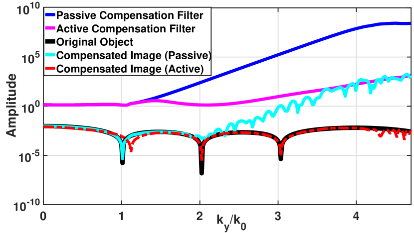
Figure 10: Fourier spectra [$Vm^{-1}$] of the reconstructed images illustrating the difference between active and passive compensation. The passive compensation has significantly amplified the noise whereas the active one does not.

Additionally, reconstructing the object features successfully requires a strong amplification. The auxiliary amplitude necessary to produce this amplification is very high and it starts to generate substantial electric field oscillations towards the edges of the image plane. Because the image plane is finite along the y-axis and the electric field is abruptly cut at a point where it is non-zero, a computational error is introduced in the spatial Fourier transform. An artefact of this can be seen in figure 10 where the red plot shows that the feature at $\frac{k_{y}}{k_{o}}=1$ is slightly shifted. The error is more prominent when the intensity of illumination is increased. Extending the size of the image plane along the y-axis mitigates the error at the expense of computational or physical resources.

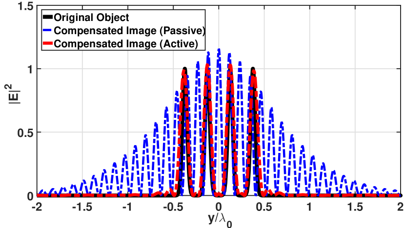
Figure 11: Reconstructed images showing the difference between active and passive compensation schemes. Note that the passively compensated image has been scaled down by $10^{7}$.

Note that towards the tails of the amplification, or when $\frac{k_{y}}{k_{o}}>4.5$, the amplification is not strong enough to overcome the noise. Hence, there should be sufficient overlap between the two adjacent auxiliaries. The FWHM of $P(k_{y})$, controlled by $\sigma$, can be selected arbitrarily. In our simulations we were limited by the finite image plane. A very narrow $P(k_{y})$ in the spatial frequency domain translates to a wide field distribution in the spatial domain. This created additional field oscillations towards the edges of the image plane increasing the errors in the Fourier transform calculations. Figure 11 shows the amplitude squared of the reconstructed fields illustrating the improvement of the active over passive compensation scheme.

V Discussion

The active compensation scheme works, because the convolved auxiliary source allows us to “selectively amplify” spatial frequency features of the object. This amplification cannot be achieved simply by the superposition of the object with an object independent auxiliary source. This is illustrated in figure 12 where we set $O(k_{y})=1Vm^{-1}$ in the second term of Eq. 6 and use the same $P(k_{y})$ distributions in figure 9. The blue and green lines correspond to the images of the object superimposed with the object independent auxiliaries with and without added noise, respectively. The buried object spectrum at $\frac{k_{y}}{k_{o}}=3$ shown in figure 9 has gone undetected.

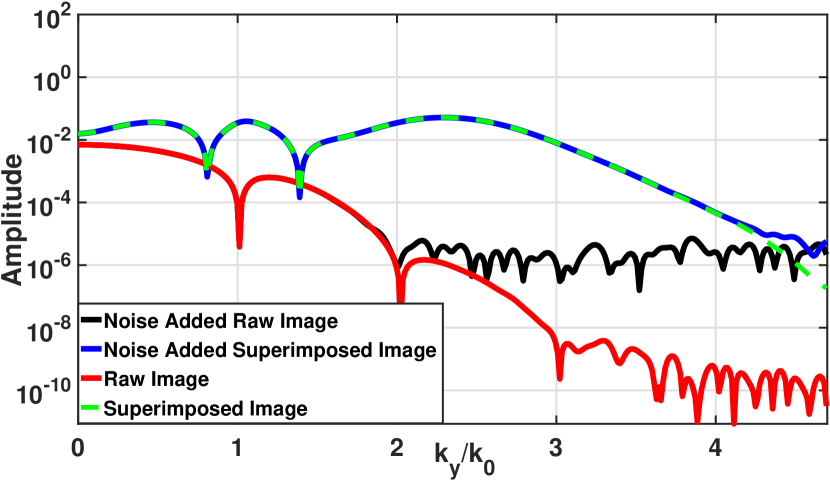
Figure 12: Fourier spectra [$Vm^{-1}$] of the raw image superimposed with several object independent auxiliaries. Such superposition does not provide amplification and hence the feature at $\frac{k_{y}}{k_{o}}=3$ is not recovered. Note that the black and red lines are the raw images with and without added noise, respectively, as also shown in figure 9.

The convolution process to construct the auxiliary source that was described in this paper can be thought of as a form of structured light illumination or wavefront engineering Zhao ; Kildishev1232009 ; Pors2013 ; PhysRevB.84.205428 ; Yu333 ; Xu:16 ; smith2003limitations ; Cao:17 . Along these lines, for example, a plasmonic lens imaging system was discussed recently in Zhao , where the authors described the fields on the image plane by Eq. 1 that contains an illumination function as a result of a phase shifting mask. Spatial filters based on hyperbolic metamaterials Rizza:12 ; schurig2003spatial ; wood2006directed may be promising for the implementation of the proposed convolution. For example, an object illuminated with a high intensity plane wave and projected on such spatial filters can physically implement the convolved auxiliary source corresponding to the second term in Eq. 6 and used in step 2 of the iterative reconstruction process. Here, the spatial filter needs to be engineered to have a transfer function of the form similar to Eq. 4. The object (i.e., such as an aperture based object illuminated by a plane wave) is to be placed on top of this additional metamaterial layer. The field distribution at the exit of this layer would be the convolution of the object field distribution with the point spread function of the layer, hence leading to the auxiliary source term in Eq. 6 (i.e., second term). One way to engineer such a transfer function is with the hyperbolic metamaterials which support high spatial frequency modes. In wood2006directed , for example, the transmission coefficient for the transverse magnetic waves in a hyperbolic medium was shown to have multiple peaks in the high spatial frequency region. The position of these peaks can be tuned by changing the filling fraction or the thickness of the hyperbolic medium. If one has engineered a metamaterial with a transfer function having one transmission peak $P_{0}$ around a certain spatial frequency (i.e., center spatial frequency $k_{c}$ in Eq. 4) and is zero everywhere else, the iterative process where $P_{0}$ is re-scaled (i.e., to control amplification) is functionally equivalent to re-scaling the amplitude of the plane wave $E_{0}$ illuminating the object. It is also worth mentioning here that this physically means actively adjusting the coherent plasmon injection rate in the imaging system to compensate the losses as conceptualized in PI . On the other hand, controlling the center frequency will require multiple or tunable metamaterial structures where the transfer function can be tuned to show transmittance peaks at different center frequencies. Therefore, it would be advantageous to have a broad transmittance in a physical implementation as long as the noise amplification does not start to dominate. Another possible way to construct the necessary transfer function may be with the use of metasurfaces Genevet:17 , which are ultrathin nanostructures fabricated at the interface of two media. The scattering properties of the sub-wavelength resonant constituents of the metasurfaces can be engineered to control the polarization, amplitude, phase, and other properties of light Kildishev1232009 ; Pors2013 ; PhysRevB.84.205428 ; Yu333 ; pfeiffer2013metamaterial ; holloway2012overview . This can allow one to engineer an arbitrary field pattern from a given incident illumination pfeiffer2013metamaterial ; holloway2012overview .

In order to understand how the active compensation enhances the resolution limit of the NIFL we need a deeper understanding of the effect of the noise on the ideal image spectrum. Eqs. 16 and 17 tell us that the signal dependent noise is amplified proportionally with the illumination. But since the active compensation seems to work so well, can we say that the noise is not amplified to the same extent as the signal? Then, would it be possible to achieve the same results by simply increasing the intensity of the plane wave illuminating the object? To address these questions we will consider below the “weak illumination,” “structured illumination” and “strong illumination” cases.

We will take the Fourier transforms of Eqs. 14 and 15 and analyze how each noise term contributes to the total distortion of the ideal image under the three illumination schemes. The linearity of the Fourier transform allows us to plot each term in the equations separately and these are shown in figures 13 - 15 for the weak, strong, and structured illuminations, respectively. In the strong illumination case we have used a plane wave whose electric field is $10^{8}$ times stronger than the weak illumination. The green and black lines in figures 13 - 15 correspond to the images with and without added noise, respectively. The Fourier transforms of the SI and SD noise are the blue and gold lines, respectively, which add up to the total noise shown by the red line.

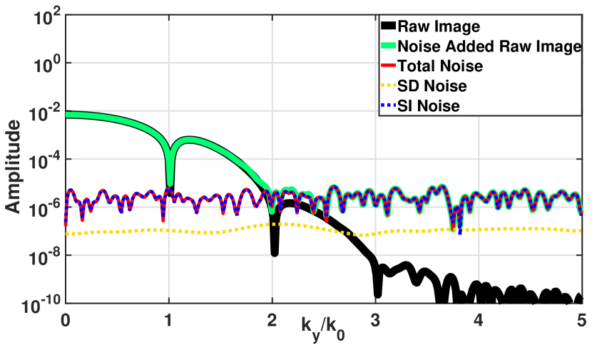
Figure 13: Fourier spectra [$Vm^{-1}$] of the raw images with and without added noise illustrating the contribution of the SD and SI noise to the total distortion of the image under the weak illumination case.

To compare the performance of the imaging system under the three illumination schemes, we will see how closely the noise added images overlap with the images with no added noise. We should note that the spatial distribution of the SD noise will be spread out over multiple Fourier components 4518410 and therefore the random nature of noise will not be visible in the spatial frequency domain. This can be seen in the gold plots which are fairly smooth compared to the blue lines.

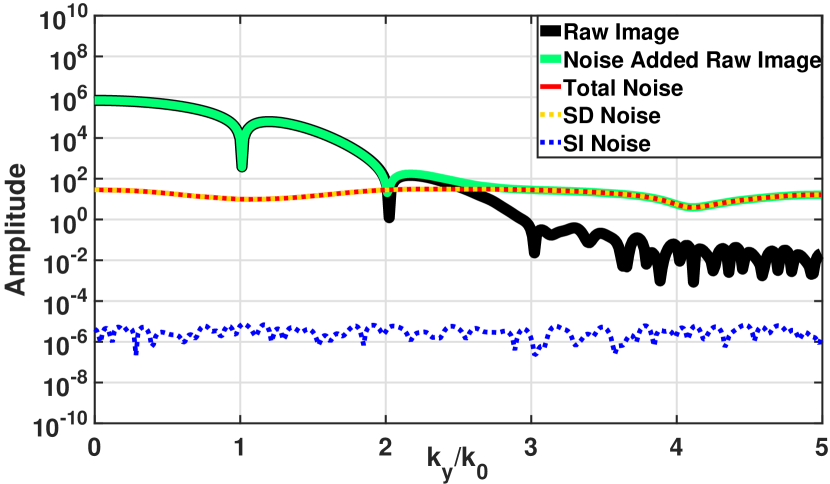
Figure 14: Fourier spectra [$Vm^{-1}$] of the raw images with and without added noise illustrating the contribution of the SD and SI noise to the total distortion of the image under the strong illumination case. The SD noise is amplified approximately by a factor of $10^{8}$ throughout the spectrum and the contribution of the SI noise is very small.

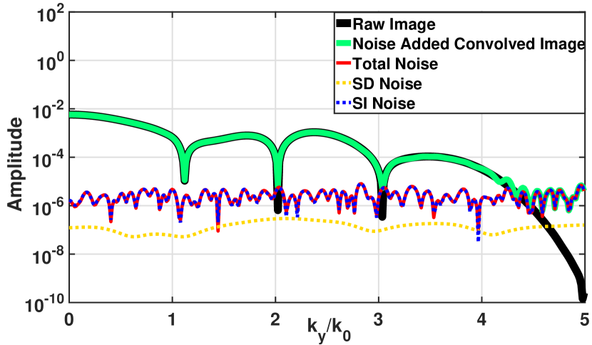
Figure 15: Fourier spectra [$Vm^{-1}$] of the convolved images with and without added noise illustrating the contribution of the SD and SI noise to the total distortion of the image under the structured illumination case. The SD noise is approximately at the same level as the weak illumination except that the noise is redistributed.

If we compare the SD noise spectra in figures 13 and 14 we immediately conclude that as we increase the intensity of the illumination, the SD noise is amplified throughout the spectrum. However, a slight improvement to the noisy spectrum over the weak illumination is visible within the region $2<\frac{k_{y}}{k_{o}}<3$. Additionally, if we analyze figure 13, where the gold line intersects the black line, we see that in the strong illumination case in figure 14, only the Fourier components until this intersection point are recovered. The intersection marks the spatial frequency at which the ideal image (i.e., raw image with no added noise) $I(k_{y})$ matches the Fourier transform of the SD noise $N_{SD}(k_{y})$. Beyond this point, we can say that the ideal image is completely buried under the SD noise alone. As we steadily increase the intensity of the illumination, $I(k_{y})$ and $N_{SD}(k_{y})$ increase by the same proportion and therefore, the value of $\frac{k_{y}}{k_{o}}$ where the two intersect does not change. We can therefore say that the improvement in the noisy spectrum in figure 14 is due to the signal rising above the SI noise which does not change with the illumination intensity. Further increments in the strength of the illumination will not improve the noisy image spectrum.

On the other hand, if we study the SD noise spectrum in figure 15, we can see that it is approximately at the same average level as figure 13. This is not surprising if we compare the green and red plots of figure 8. We can see that the spatial electric field distribution of the noise added images $I^{{}^{\prime}}_{N}(y)$ and $I_{N}(y)$ are comparable. The only difference is that $I^{{}^{\prime}}_{N}(y)$ has high spatial frequency features. Since the standard deviation of the SD noise is proportional to the amplitude of the image, according to Eqs. 16 and 17, we can see why the SD noise is approximately the same in both the weak and structured illumination schemes. Note that under the structured illumination, the noise added convolved image closely follows the ideal image until $\frac{k_{y}}{k_{o}}=4.5$. This can be pushed to even higher spatial frequencies if the transfer function characterizing the lens is accurate. Also, note that the structured illumination has successfully suppressed the computational errors in the Fourier transform which are visible in the black line in figure 13 beyond $\frac{k_{y}}{k_{o}}=3$. These errors are amplified by a factor of $10^{8}$ times in figure 14.

From the above discussion we conclude that by using structured illumination the SD noise is not amplified but redistributed when compared with the strong illumination. Therefore, it is possible to raise the high spatial frequency features of the object above the noise. This is the primary reason why structured illumination can accurately resolve the image while strong illumination fails.

The technique is generally applicable to any arbitrary object with the use of any plasmonic or metamaterial lens provided that accurate transfer function for the imaging system is available. A selective amplification process is used to recover specific object features by controlling $P_{0}$ near and beyond where the noise floor is reached in the Fourier spectrum of the raw image. Therefore, no prior knowledge of the object is required. However, a necessary criterion is a sufficiently accurate transfer function in the region where the auxiliary is applied to correctly estimate the required amount of amplification. It should be noted that different objects may require different auxiliaries, since the spatial frequency at which the noise floor is reached may vary for different objects. Therefore, it would be instrumental to have a tunability mechanism for the versatility of the imaging system. Even though a single narrowband auxiliary would be still sufficient to enhance the resolution of the raw image, further enhancement in the resolution would demand either superimposing multiple narrowband auxiliaries or a single sufficiently broadband auxiliary within the range of accurate transfer function. Narrowband auxiliaries require larger image plane and more post-processing while a single broadband auxiliary requires less post-processing and smaller image plane at the expense of possibly higher noise amplification. Similarly, unnecessarily large amplitude of a narrowband auxiliary may excessively amplify the noise. Another likely limitation arises from increasingly large power loss in the deep subwavelength regime, which requires increasingly high amount of amplification to reconstruct extremely fine details of the object. This does not only reduce the efficiency but might also introduce undesired non-linear and thermal effects in the optical materials, hence, limiting the resolution of the imaging system.

VI Conclusion

In summary, we proposed an active implementation of the recently introduced plasmon injection scheme PI to significantly improve the resolution of Pendry’s non-ideal negative index flat lens beyond diffraction limit in the presence of realistic material losses and SD noise. Simply by increasing the illumination intensity, it is not generally possible to efficiently reconstruct the image due to the noise amplification. However, in the proposed active implementation one can counter the adverse noise amplification effect by using a convolved auxiliary source which allows for a selective amplification of the high spatial frequency features deep within the sub-wavelength regime. We have shown that this approach can be used to control the noise amplification while at the same time recover features buried within the noise, thus enabling ultra-high resolution imaging far beyond the previous passive implementations of the plasmon injection scheme Wyatt ; zhang2016enhancing . The convolution process to construct the auxiliary source in the proposed active scheme may be realized physically by different methods, metasurfaces Genevet:17 ; Kildishev1232009 ; Pors2013 ; PhysRevB.84.205428 ; Yu333 ; Xu:16 ; pfeiffer2013metamaterial ; holloway2012overview and hyperbolic metamaterials Rizza:12 ; schurig2003spatial ; wood2006directed ; zhang2015hyperbolic being the primary candidates. A more detailed analysis on the design of such structures to implement the convolved auxiliary source will be the focus of our future research. Finally, we should note that we purposefully focused on imperfect negative index flat lens here that poses a highly stringent and conservative problem. However, in the shorter term the proposed method can be relatively easily applied to experimentally available plasmonic superlenses Guo2014 ; Liu_Hong ; Zhao ; Fang534 ; taubner2006near ; zhang2008superlenses and hyperlenses liu2007far ; rho2010spherical ; lu2012hyperlenses ; sun2015experimental ; lee2007development . Our findings also raises the hopes for reviving Pendry’s early vision of perfect lens Pendry by decoupling the loss and isotropy issues toward a practical realization soukoulis2010optical ; soukoulis2011past ; guney2009connected ; guney2010intra ; rudolph2012broadband ; yang2016experimental .

VII Funding Information

Office of Naval Research (award N00014-15-1-2684).

VIII Acknowledgement

We thank Jeremy Bos at Michigan Technological University for fruitful discussion on noise characterization.

References

- (1) N. Fang, H. Lee, C. Sun, and X. Zhang, “Diffraction-limited optical imaging with a silver superlens,” Science 308, 534–537 (2005).
- (2) T. Taubner, D. Korobkin, Y. Urzhumov, G. Shvets, and R. Hillenbrand, “Near-field microscopy through a sic superlens,” Science 313, 1595–1595 (2006).
- (3) X. Zhang and Z. Liu, “Superlenses to overcome the diffraction limit,” Nature materials 7, 435–441 (2008).
- (4) Z. Liu, H. Lee, Y. Xiong, C. Sun, and X. Zhang, “Far-field optical hyperlens magnifying sub-diffraction-limited objects,” science 315, 1686–1686 (2007).
- (5) J. Rho, Z. Ye, Y. Xiong, X. Yin, Z. Liu, H. Choi, G. Bartal, and X. Zhang, “Spherical hyperlens for two-dimensional sub-diffractional imaging at visible frequencies,” Nature communications 1, 143 (2010).
- (6) D. Lu and Z. Liu, “Hyperlenses and metalenses for far-field super-resolution imaging,” Nature communications 3, 1205 (2012).
- (7) J. Sun, M. I. Shalaev, and N. M. Litchinitser, “Experimental demonstration of a non-resonant hyperlens in the visible spectral range,” Nature communications 6, 7201 (2015).
- (8) H. Lee, Z. Liu, Y. Xiong, C. Sun, and X. Zhang, “Development of optical hyperlens for imaging below the diffraction limit,” Optics express 15, 15886–15891 (2007).
- (9) J. Valentine, S. Zhang, T. Zentgraf, E. Ulin-Avila, D. A. Genov, G. Bartal, and X. Zhang, “Three-dimensional optical metamaterial with a negative refractive index,” nature 455, 376–379 (2008).
- (10) N. I. Landy, S. Sajuyigbe, J. Mock, D. Smith, and W. Padilla, “Perfect metamaterial absorber,” Physical review letters 100, 207402 (2008).
- (11) V. V. Temnov, “Ultrafast acousto-magneto-plasmonics,” Nature Photonics 6, 728–736 (2012).
- (12) M. I. Aslam and D. Ö. Güney, “On negative index metamaterial spacers and their unusual optical properties,” Progress in Electromagnetic Research B 6, 203–217 (2013).
- (13) M. Sadatgol, M. Rahman, E. Forati, M. Levy, and D. Ö. Güney, “Enhanced faraday rotation in hybrid magneto-optical metamaterial structure of bismuth-substituted-iron-garnet with embedded-gold-wires,” Journal of Applied Physics 119, 103105 (2016).
- (14) M. Choi, S. H. Lee, Y. Kim, S. B. Kang, J. Shin, M. H. Kwak, K.-Y. Kang, Y.-H. Lee, N. Park, and B. Min, “A terahertz metamaterial with unnaturally high refractive index,” Nature 470, 369–373 (2011).
- (15) W.-C. Chen, C. M. Bingham, K. M. Mak, N. W. Caira, and W. J. Padilla, “Extremely subwavelength planar magnetic metamaterials,” Physical Review B 85, 201104 (2012).
- (16) X. Zhang, E. Usi, S. K. Khan, M. Sadatgol, and D. Ö. Guney, “Extremely sub-wavelength negative index metamaterial,” Progress In Electromagnetics Research 152, 95–104 (2015).
- (17) D. Schurig, J. Mock, B. Justice, S. A. Cummer, J. B. Pendry, A. Starr, and D. Smith, “Metamaterial electromagnetic cloak at microwave frequencies,” Science 314, 977–980 (2006).
- (18) J. Gwamuri, D. Güney, and J. Pearce, “Advances in plasmonic light trapping in thin-film solar photovoltaic devices,” Solar cell nanotechnology pp. 241–269 (2013).
- (19) C. Rockstuhl, S. Fahr, and F. Lederer, “Absorption enhancement in solar cells by localized plasmon polaritons,” Journal of applied physics 104, 123102 (2008).
- (20) A. Vora, J. Gwamuri, N. Pala, A. Kulkarni, J. M. Pearce, and D. Ö. Güney, “Exchanging ohmic losses in metamaterial absorbers with useful optical absorption for photovoltaics,” Scientific Reports 4, 4901 (2008).
- (21) A. Vora, J. Gwamuri, J. M. Pearce, P. L. Bergstrom, and D. Ö. Güney, “Multi-resonant silver nano-disk patterned thin film hydrogenated amorphous silicon solar cells for staebler-wronski effect compensation,” Journal of Applied Physics 116, 093103 (2014).
- (22) I. Bulu, H. Caglayan, K. Aydin, and E. Ozbay, “Compact size highly directive antennas based on the srr metamaterial medium,” New Journal of Physics 7, 223 (2005).
- (23) H. Odabasi, F. Teixeira, and D. Guney, “Electrically small, complementary electric-field-coupled resonator antennas,” Journal of Applied Physics 113, 084903 (2013).
- (24) D. Ö. Güney and D. A. Meyer, “Negative refraction gives rise to the klein paradox,” Physical Review A 79, 063834 (2009).
- (25) I. I. Smolyaninov and E. E. Narimanov, “Metric signature transitions in optical metamaterials,” Physical Review Letters 105, 067402 (2010).
- (26) M. S. Tame, K. McEnery, Ş. Özdemir, J. Lee, S. Maier, and M. Kim, “Quantum plasmonics,” Nature Physics 9, 329–340 (2013).
- (27) M. A. al Farooqui, J. Breeland, M. I. Aslam, M. Sadatgol, Ş. K. Özdemir, M. Tame, L. Yang, and D. Ö. Güney, “Quantum entanglement distillation with metamaterials,” Optics express 23, 17941–17954 (2015).
- (28) M. Asano, M. Bechu, M. Tame, Ş. K. Özdemir, R. Ikuta, D. Ö. Güney, T. Yamamoto, L. Yang, M. Wegener, and N. Imoto, “Distillation of photon entanglement using a plasmonic metamaterial,” Scientific reports 5, 18313 (2015).
- (29) P. K. Jha, X. Ni, C. Wu, Y. Wang, and X. Zhang, “Metasurface-enabled remote quantum interference,” Physical review letters 115, 025501 (2015).
- (30) R. A. Sperling, P. R. Gil, F. Zhang, M. Zanella, and W. J. Parak, “Biological applications of gold nanoparticles,” Chemical Society Reviews 37, 1896–1908 (2008).
- (31) X. Huang, I. H. El-Sayed, W. Qian, and M. A. El-Sayed, “Cancer cell imaging and photothermal therapy in the near-infrared region by using gold nanorods,” Journal of the American Chemical Society 128, 2115–2120 (2006).
- (32) S. Lal, S. E. Clare, and N. J. Halas, “Nanoshell-enabled photothermal cancer therapy: impending clinical impact,” Accounts of chemical research 41, 1842–1851 (2008).
- (33) R. Guo, L. Zhang, H. Qian, R. Li, X. Jiang, and B. Liu, “Multifunctional nanocarriers for cell imaging, drug delivery, and near-ir photothermal therapy,” Langmuir 26, 5428–5434 (2010).
- (34) Z. J. Coppens, W. Li, D. G. Walker, and J. G. Valentine, “Probing and controlling photothermal heat generation in plasmonic nanostructures,” Nano Letters 13, 1023–1028 (2013).
- (35) M. D. Blankschien, L. A. Pretzer, R. Huschka, N. J. Halas, R. Gonzalez, and M. S. Wong, “Light-triggered biocatalysis using thermophilic enzyme–gold nanoparticle complexes,” ACS nano 7, 654–663 (2012).
- (36) Y.-S. Chen, W. Frey, S. Kim, K. Homan, P. Kruizinga, K. Sokolov, and S. Emelianov, “Enhanced thermal stability of silica-coated gold nanorods for photoacoustic imaging and image-guided therapy,” Optics express 18, 8867–8878 (2010).
- (37) S. P. Sherlock, S. M. Tabakman, L. Xie, and H. Dai, “Photothermally enhanced drug delivery by ultra-small multifunctional feco/graphitic-shell nanocrystals,” Acs Nano 5, 1505 (2011).
- (38) A. Ahmadivand, N. Pala, and D. Ö. Güney, “Enhancement of photothermal heat generation by metallodielectric nanoplasmonic clusters,” Optics express 23, A682–A691 (2015).
- (39) J. B. Pendry, “Negative refraction makes a perfect lens,” Phys. Rev. Lett. 85, 3966–3969 (2000).
- (40) W. Adams, M. Sadatgol, and D. Ö. Güney, “Review of near-field optics and superlenses for sub-diffraction-limited nano-imaging,” AIP Advances 6, 100701 (2016).
- (41) S. Zhang, W. Fan, N. C. Panoiu, K. J. Malloy, R. M. Osgood, and S. R. J. Brueck, “Experimental demonstration of near-infrared negative-index metamaterials,” Phys. Rev. Lett. 95, 137404 (2005).
- (42) A. N. Grigorenko, A. K. Geim, H. F. Gleeson, Y. Zhang, A. A. Firsov, I. Y. Khrushchev, and J. Petrovic, “Nanofabricated media with negative permeability at visible frequencies,” Nature 438, 335–338 (2005).
- (43) G. Dolling, C. Enkrich, M. Wegener, C. M. Soukoulis, and S. Linden, “Simultaneous negative phase and group velocity of light in a metamaterial,” Science 312, 892–894 (2006).
- (44) K. J. Webb, M. Yang, D. W. Ward, and K. A. Nelson, “Metrics for negative-refractive-index materials,” Phys. Rev. E 70, 035602 (2004).
- (45) M.-C. Yang and K. J. Webb, “Poynting vector analysis of a superlens,” Opt. Lett. 30, 2382–2384 (2005).
- (46) M. P. Nezhad, K. Tetz, and Y. Fainman, “Gain assisted propagation of surface plasmon polaritons on planar metallic waveguides,” Opt. Express 12, 4072–4079 (2004).
- (47) A. K. Popov and V. M. Shalaev, “Compensating losses in negative-index metamaterials by optical parametric amplification,” Opt. Lett. 31, 2169–2171 (2006).
- (48) D. O. Güney, T. Koschny, and C. M. Soukoulis, “Reducing ohmic losses in metamaterials by geometric tailoring,” Phys. Rev. B 80, 125129 (2009).
- (49) S. Anantha Ramakrishna and J. B. Pendry, “Removal of absorption and increase in resolution in a near-field lens via optical gain,” Phys. Rev. B 67, 201101 (2003).
- (50) Zhang, J., Jiang, H., Gralak, B., Enoch, S., Tayeb, G., and Lequime, M., “Compensation of loss to approach –1 effective index by gain in metal-dielectric stacks,” Eur. Phys. J. Appl. Phys. 46, 32603 (2009).
- (51) M. I. Stockman, “Criterion for negative refraction with low optical losses from a fundamental principle of causality,” Phys. Rev. Lett. 98, 177404 (2007).
- (52) M. Sadatgol, K. Özdemir, L. Yang, and D. O. Güney, “Plasmon injection to compensate and control losses in negative index metamaterials,” Phys. Rev. Lett. 115, 035502 (2015).
- (53) M. I. Aslam and D. O. Güney, “Surface plasmon driven scalable low-loss negative-index metamaterial in the visible spectrum,” Phys. Rev. B 84, 195465 (2011).
- (54) D. Ö. Güney, T. Koschny, and C. M. Soukoulis, “Surface plasmon driven electric and magnetic resonators for metamaterials,” Physical Review B 83, 045107 (2011).
- (55) M. I. Aslam and D. Ö. Güney, “Dual-band, double-negative, polarization-independent metamaterial for the visible spectrum,” JOSA B 29, 2839–2847 (2012).
- (56) W. Adams, M. Sadatgol, X. Zhang, and D. O. Güney, “Bringing the ‘perfect lens’ into focus by near-perfect compensation of losses without gain media,” New Journal of Physics 18, 125004 (2016).
- (57) T. Xu, A. Agrawal, M. Abashin, K. J. Chau, and H. J. Lezec, “All-angle negative refraction and active flat lensing of ultraviolet light,” Nature 497, 470–474 (2013).
- (58) C. García-Meca, J. Hurtado, J. Martí, A. Martínez, W. Dickson, and A. V. Zayats, “Low-loss multilayered metamaterial exhibiting a negative index of refraction at visible wavelengths,” Phys. Rev. Lett. 106, 067402 (2011).
- (59) E. Verhagen, R. de Waele, L. Kuipers, and A. Polman, “Three-dimensional negative index of refraction at optical frequencies by coupling plasmonic waveguides,” Phys. Rev. Lett. 105, 223901 (2010).
- (60) Y. Chen, Y.-C. Hsueh, M. Man, and K. J. Webb, “Enhanced and tunable resolution from an imperfect negative refractive index lens,” J. Opt. Soc. Am. B 33, 445–451 (2016).
- (61) R. D. Fiete and T. Tantalo, “Comparison of snr image quality metrics for remote sensing systems,” Optical Engineering 40, 574–585 (2001).
- (62) M. N. Wernick, O. Wirjadi, D. Chapman, Z. Zhong, N. P. Galatsanos, Y. Yang, J. G. Brankov, O. Oltulu, M. A. Anastasio, and C. Muehleman, “Multiple-image radiography,” Physics in Medicine and Biology 48, 3875 (2003).
- (63) G. T. Barnes, “Radiographic mottle: A comprehensive theory,” Medical Physics 9, 656–667 (1982).
- (64) Z. Guo, Q. Huang, C. Wang, P. Gao, W. Zhang, Z. Zhao, L. Yan, and X. Luo, “Negative and positive impact of roughness and loss on subwavelength imaging for superlens structures,” Plasmonics 9, 103–110 (2014).
- (65) H. Wang, J. Q. Bagley, L. Tsang, S. Huang, K.-H. Ding, and A. Ishimaru, “Image enhancement for flat and rough film plasmon superlenses by adding loss,” J. Opt. Soc. Am. B 28, 2499–2509 (2011).
- (66) H. Liu, B. Wang, L. Ke, J. Deng, C. C. Choy, M. S. Zhang, L. Shen, S. A. Maier, and J. H. Teng, “High contrast superlens lithography engineered by loss reduction,” Advanced Functional Materials 22, 3777–3783 (2012).
- (67) G. C. Holst, “Ccd arrays, cameras, and displays,” (1998).
- (68) J. F. Walkup and R. C. Choens, “Image processing in signal-dependent noise,” Optical Engineering 13, 133258–133258 (1974).
- (69) J. J. Heine and M. Behera, “Aspects of signal-dependent noise characterization,” J. Opt. Soc. Am. A 23, 806–815 (2006).
- (70) R. Kasturi, J. F. Walkup, and T. F. Krile, “Image restoration by transformation of signal-dependent noise to signal-independent noise,” Appl. Opt. 22, 3537–3542 (1983).
- (71) G. K. Froehlich, J. F. Walkup, and T. F. Krile, “Estimation in signal-dependent film-grain noise,” Appl. Opt. 20, 3619–3626 (1981).
- (72) M. Akiba, K. Tsujino, and M. Sasaki, “Ultrahigh-sensitivity single-photon detection with linear-mode silicon avalanche photodiode,” Opt. Lett. 35, 2621–2623 (2010).
- (73) Z. Zhao, Y. Luo, N. Yao, W. Zhang, C. Wang, P. Gao, C. Zhao, M. Pu, and X. Luo, “Modeling and experimental study of plasmonic lens imaging with resolution enhanced methods,” Opt. Express 24, 27115–27126 (2016).
- (74) A. V. Kildishev, A. Boltasseva, and V. M. Shalaev, “Planar photonics with metasurfaces,” Science 339 (2013).
- (75) A. Pors, M. G. Nielsen, R. L. Eriksen, and S. I. Bozhevolnyi, “Broadband focusing flat mirrors based on plasmonic gradient metasurfaces,” Nano Letters 13, 829–834 (2013).
- (76) Y. Zhao and A. Alù, “Manipulating light polarization with ultrathin plasmonic metasurfaces,” Phys. Rev. B 84, 205428 (2011).
- (77) N. Yu, P. Genevet, M. A. Kats, F. Aieta, J.-P. Tetienne, F. Capasso, and Z. Gaburro, “Light propagation with phase discontinuities: Generalized laws of reflection and refraction,” Science 334, 333–337 (2011).
- (78) Y. Xu, J. Sun, W. Walasik, and N. M. Litchinitser, “Probing metamaterials with structured light,” Opt. Express 24, 26249–26254 (2016).
- (79) D. R. Smith, D. Schurig, M. Rosenbluth, S. Schultz, S. A. Ramakrishna, and J. B. Pendry, “Limitations on subdiffraction imaging with a negative refractive index slab,” Applied Physics Letters 82, 1506–1508 (2003).
- (80) S. Cao, T. Wang, Q. Sun, B. Hu, and W. Yu, “Meta-nanocavity model for dynamic super-resolution fluorescent imaging based on the plasmonic structure illumination microscopy method,” Opt. Express 25, 3863–3874 (2017).
- (81) C. Rizza, A. Ciattoni, E. Spinozzi, and L. Columbo, “Terahertz active spatial filtering through optically tunable hyperbolic metamaterials,” Opt. Lett. 37, 3345–3347 (2012).
- (82) D. Schurig and D. R. Smith, “Spatial filtering using media with indefinite permittivity and permeability tensors,” Applied Physics Letters 82, 2215–2217 (2003).
- (83) B. Wood, J. Pendry, and D. Tsai, “Directed subwavelength imaging using a layered metal-dielectric system,” Physical Review B 74, 115116 (2006).
- (84) P. Genevet, F. Capasso, F. Aieta, M. Khorasaninejad, and R. Devlin, “Recent advances in planar optics: from plasmonic to dielectric metasurfaces,” Optica 4, 139–152 (2017).
- (85) C. Pfeiffer and A. Grbic, “Metamaterial huygens’ surfaces: tailoring wave fronts with reflectionless sheets,” Physical review letters 110, 197401 (2013).
- (86) C. L. Holloway, E. F. Kuester, J. A. Gordon, J. O’Hara, J. Booth, and D. R. Smith, “An overview of the theory and applications of metasurfaces: The two-dimensional equivalents of metamaterials,” IEEE Antennas and Propagation Magazine 54, 10–35 (2012).
- (87) K. Hirakawa, “Fourier and filterbank analyses of signal-dependent noise,” in “2008 IEEE International Conference on Acoustics, Speech and Signal Processing,” (2008), pp. 3517–3520.
- (88) X. Zhang, W. Adams, M. Sadatgol, and D. Ö. Güney, “Enhancing the resolution of hyperlens by the compensation of losses without gain media,” Progress in Electromagnetic Research C 70, 1–7 (2016).
- (89) X. Zhang, S. Debnath, and D. Ö. Güney, “Hyperbolic metamaterial feasible for fabrication with direct laser writing processes,” JOSA B 32, 1013–1021 (2015).
- (90) C. M. Soukoulis and M. Wegener, “Optical metamaterials—more bulky and less lossy,” Science 330, 1633–1634 (2010).
- (91) C. M. Soukoulis and M. Wegener, “Past achievements and future challenges in the development of three-dimensional photonic metamaterials,” Nature Photonics 5, 523–530 (2011).
- (92) D. Ö. Güney, T. Koschny, M. Kafesaki, and C. M. Soukoulis, “Connected bulk negative index photonic metamaterials,” Optics letters 34, 506–508 (2009).
- (93) D. Ö. Güney, T. Koschny, and C. M. Soukoulis, “Intra-connected three-dimensionally isotropic bulk negative index photonic metamaterial,” Optics express 18, 12348–12353 (2010).
- (94) S. M. Rudolph and A. Grbic, “A broadband three-dimensionally isotropic negative-refractive-index medium,” IEEE Transactions on Antennas and Propagation 60, 3661–3669 (2012).
- (95) S. Yang, X. Ni, B. Kante, J. Zhu, K. O’Brien, Y. Wang, and X. Zhang, “Experimental demonstration of optical metamaterials with isotropic negative index,” in “Lasers and Electro-Optics (CLEO), 2016 Conference on,” (IEEE, 2016), pp. 1–2.