Lunar Mass Black Holes from QCD Axion Cosmology

Abstract

In the QCD axion scenario, a network of domain walls bounded by cosmic strings fragments into pieces. As these fragments collapse, some of them will form black holes. With standard QCD axion parameters, the black holes will have lunar masses ($M_{\rm bh}\sim 10^{-8}\,{\rm M}_{\odot}$). Even though their number density is difficult to estimate, arguments suggest that they can constitute a reasonable fraction of the critical cosmological density.

Note: More recent simulations Fleury and Moore (2016) show that the string-wall network will fragment earlier than what is estimated below. Then the wall pieces will be smaller and the chance of forming a black hole will be lower. Thus the QCD axion scenario is unlikely to lead to an interesting number of black holes. However other axion models, with different parameters and cosmological evolution, might lead to black holes in larger numbers and the physics discussed in this paper could still be of interest.

The axion was proposed as a way to understand the smallness of the neutron electric dipole moment even when theoretical considerations would suggest a large value. (For a review see Kim and Carosi (2010)). An unexpected benefit is that axions can play the role of cold dark matter in cosmology Marsh (2016). At the same time, an unintended consequence of the QCD axion model is the existence of a network of cosmic strings in the early universe, at temperatures above the QCD scale. At the QCD scale additional domain walls are created that connect the strings in the network. In the usual picture the domain walls shrink and cause the network to collapse and annihilate into axion radiation, thus leaving no consequential signature of their one time existence Vilenkin and Everett (1982); Kibble et al. (1982). In this paper we point out that the collapse of the string network can also produce lunar mass black holes. However, their number density is difficult to estimate. The arguments are similar to those already given for black hole formation from collapsing cosmic string loops Hawking (1990); Fort and Vachaspati (1993) and also from domain walls produced during inflation Deng et al. (2017); Rubin et al. (2001).

The timeline of the QCD axion starts at the so-called Peccei-Quinn energy scale, $f_{\rm PQ}$, when a global U(1) symmetry breaks spontaneously to the trivial group. The phase of the Peccei-Quinn complex scalar field is a Goldstone boson and is called the axion. The U(1) symmetry breaking generates a network of cosmic global strings (reviewed in Vilenkin and Shellard (2000)). The tension of the global strings, $\mu$, is given by

$$\mu\approx\pi\,\ln(f_{\rm PQ}L)f_{\rm PQ}^{2}$$ (1)

where $L$ is the typical inter-string separation and is bounded by the cosmic horizon and $f_{\rm PQ}$ is taken to be the vacuum expectation value of the Peccei-Quinn complex scalar field. The logarithmic factor is weakly dependent on the length $L$. For example, if $L$ is of order the horizon at the QCD temperature, $t_{\rm QCD}\approx 10^{-3}~{}{\rm s}$, and $f_{\rm PQ}\approx 10^{11}~{}{\rm GeV}$, we have $\ln(f_{\rm PQ}L)\approx 70$.

The Peccei-Quinn scale, $f_{\rm PQ}$, is constrained by cosmology Hagmann et al. (2001); Wantz and Shellard (2010a); Hiramatsu et al. (2012); Visinelli and Gondolo (2014); Klaer and Moore (2017) to be between $10^{10}-10^{12}~{}{\rm GeV}$ and we will take

$$f_{\rm PQ}=3\times 10^{10}\,{\rm GeV}\,f_{*}$$ (2)

with $f_{*}\approx 1$ a free parameter.

The string network evolves under the forces of string tension, Hubble expansion, and backreaction from Goldstone boson radiation; the network also reconfigures itself due to intercommutations when strings intersect. The Goldstone boson radiation from global strings is quite efficient Vilenkin and Vachaspati (1987) and we expect the long strings to not be very curved. The typical coherence scale of the strings will be assumed to be on the cosmic horizon scale.

The string network evolves freely until the cosmic temperature drops to about the QCD energy scale, $\Lambda_{\rm QCD}\approx 200\,{\rm MeV}$ when the axions rapidly acquire a mass Wantz and Shellard (2010b); Borsanyi et al. (2016). Ref. Wantz and Shellard (2010b) gives a convenient formula for the axion mass as a function of cosmic temperature,

$$m_{a}^{2}(T)\frac{f_{\rm PQ}^{2}}{\Lambda^{4}}=\begin{cases}1.46\times 10^{-3}\frac{1+0.5x}{1+(3.53\,x)^{7.48}},&x<1.125\\ \\ 1.68\times 10^{-7}x^{-6.68},&x\geq 1.125\end{cases}$$ (3)

where $x\equiv T/\Lambda$, $\Lambda=400~{}{\rm MeV}\equiv 2\Lambda_{\rm QCD}$. In Fig. 1 we plot the temperature dependence of the axion mass.

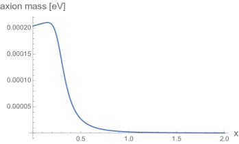
Figure 1: Mass of axion in eV versus $x=T/\Lambda$ for $f_{\rm PQ}=3\times 10^{10}~{}{\rm GeV}$ Wantz and Shellard (2010b).

The temperature dependence causes the axion mass to turn on in time at about the QCD cosmological epoch. To determine the time-dependence we use the cosmic time-temperature relation,

$$\frac{1}{4t^{2}}=H^{2}=\frac{8\pi G}{3}\frac{\pi^{2}}{30}g_{*}T^{4}$$ (4)

where $g_{*}\approx 70$ counts the relativistic degrees of freedom. This gives,

$$\frac{1}{t}=27.8\frac{T^{2}}{m_{P}}$$ (5)

where the Planck mass $m_{P}=1.22\times 10^{19}~{}{\rm GeV}$.

With a non-zero mass of the axion, the phase of the complex scalar field, namely the axion denoted by the field $a$, develops a potential that is approximately described by the sine-Gordon potential. The Lagrangian is

$$L=f_{\rm PQ}^{2}\left[\frac{1}{2}(\partial_{\mu}a)^{2}-m_{a}^{2}(1-\cos(a))\right]$$ (6)

The potential is periodic under $a\to a+2\pi n$ where $n$ is any integer. Thus there are domain wall solutions that interpolate between the minima of the potential. The wall tension (energy per unit area) in the sine-Gordon model is

$$\sigma=8m_{a}f_{\rm PQ}^{2}.$$ (7)

A precision analysis shows slight departures of the true axion potential from the sine-Gordon model Grilli di Cortona et al. (2016) and that the correct wall tension is $8.97\,m_{a}f_{\rm PQ}^{2}$. We will disregard this small difference and continue to describe axion dynamics by the sine-Gordon model.

There are three relevant epochs for the evolution. First is the time, denoted $t_{H}$, when the tension in the axion walls starts to dominate over the Hubble expansion. This is given by $m_{a}(t_{H})t_{H}=1$ and we find that the temperature at this epoch is $T_{H}\simeq 2~{}{\rm GeV}$. This is also the time at which the force on the network due to domain walls becomes more important than the tension in horizon-size strings i.e. $\sigma>\mu/t$. A second relevant time is when the string-wall network fragments into isolated pieces. We will denote this time $t_{\rm f}$ and $t_{\rm f}>t_{H}$ because the tension in the walls has to overcome Hubble expansion for the network to fragment. A third relevant time, denoted $t_{a}$, is when the axion has acquired its asymptotic mass. From the plot of $m_{a}(T)$ in Fig. 1 we see that this happens at a temperature $T_{a}\approx 0.2\Lambda$. The numerical values for $T_{a}$ and the corresponding epoch are

$$T_{a}\approx 0.2\Lambda\approx 80~{}{\rm MeV},\ \ t_{a}\approx 4.5\times 10^{-5}~{}{\rm s}$$ (8)

and the axion mass from this time on is,

$$m_{a,0}\approx 2.0\times 10^{-4}~{}{\rm eV}\ f_{*}^{-1}$$ (9)

The next task will be to estimate $t_{\rm f}$. Early simulations of the string-wall network performed in Ref. Hiramatsu et al. (2012) indicate that the network does not fragment until after $t_{a}$ (see Figs. 2 and 4 of Ref. Hiramatsu et al. (2012)). However, the more recent analysis of Ref. Klaer and Moore (2017) shows earlier fragmentation at a time $\sim 0.1t_{a}$. check

The estimates in Eqs. (8) and (9) also give

$$m_{a,0}t_{a}\sim 1.4\times 10^{7}\,f_{*}^{-1}$$ (10)

which says that the size $\sim t_{a}$ of the walls is much larger than their width $\sim m_{a}^{-1}$.

Once the network has fragmented, the pieces, that we call “membranes”, start to collapse due to tension and may collapse into black holes. However, a membrane will also lose energy into radiation as it collapses. Then there is competition between the rate of collapse and the rate of radiation. This process has been considered for local cosmic strings Hawking (1990) and for global cosmic string loops Fort and Vachaspati (1993). For circular gauge cosmic strings, the dominant emission is to gravitational radiation. This is quite weak and leads to a significant range of parameters that can give black holes. For circular global cosmic string loops, Goldstone boson radiation is very efficient and the parameter space for black hole formation is very restricted. However, since the axion has a mass, our membranes are not like global strings and black hole formation requires a separate study. We will first give a rough estimate for when black holes can form and then analyze the collapse of spherical sine-Gordon walls in more detail (similar to the analysis in Ref. Widrow (1989) for $Z_{2}$ walls).

Consider a membrane in the shape of a circular disk that starts contracting from an initial radius $R_{0}$ that is close to the horizon size $t_{a}$. To form a black hole, the membrane must collapse so that its radius at some later time $t_{\rm bh}$ satisfies $R(t_{\rm bh})=2GM$ where $M=\sigma\pi R_{0}^{2}$ and $\sigma$ is the wall tension in Eq. (7) with $m_{a}$ replaced by $m_{a,0}$. However, there is also a second constraint: the Schwarzschild radius $R(t_{\rm bh})$ must be larger than the width of the wall $\sim m_{a,0}^{-1}$, otherwise radiation will become important once $R(t)<m_{a,0}^{-1}$ as discussed in Fort and Vachaspati (1993). Therefore the condition for black hole formation is

$$2G\sigma\pi R_{0}^{2}>R(t_{\rm bh})\gtrsim m_{a,0}^{-1}.$$ (11)

This condition is to be taken as a rough guide. For example, the $m_{a,0}^{-1}$ on the right-hand side ignores the Lorentz contraction of the wall and string as the system collapses. For a disk membrane, this will make the string thinner by the inverse of the boost factor but the wall thickness will not change; for a spherical wall, the wall will get Lorentz contracted. We continue with Eq. (11) for now, as it may be more relevant to the case of a circular disk, but will do a more careful numerical analysis for a collapsing spherical wall below. The black hole formation condition can also be written as

$$\frac{R_{0}}{t_{a}}\gtrsim\frac{1}{\sqrt{18\pi}}\frac{m_{P}}{m_{a,0}t_{a}f_{\rm PQ}}\simeq 4$$ (12)

This estimate shows that we do not expect black hole formation in general. However, the estimate is close enough that we expect black holes to form with some reduced probability. For example, geometric factors for the shape of the wall can contribute to this condition – we could have considered a membrane with a larger surface area than that of a disk. Also, the typical scale of the network may be set by the Hubble scale instead of the cosmic time which would make the initial size somewhat bigger than $t_{a}$. And the membranes might at first be stretched due to Hubble flow which would also make them bigger.

The above estimate gives us a rough idea for when black holes will form. We can examine the particular case of collapse of a spherical domain wall in much greater detail by numerically solving its equation of motion,

$$\partial_{t}^{2}a=\nabla^{2}a-\sin(a)$$ (13)

where we have set $m_{a,0}=1$ by rescaling coordinates. The initial field for the spherical domain wall can be written as Vachaspati (2010)

$$a(t=0,r)=4[\tan^{-1}(e^{r+R_{0}})+\tan^{-1}(e^{-r+R_{0}})]-2\pi$$ (14)

where $r$ is the (rescaled) spherical radial coordinate. We also start with a static spherical wall so ${\dot{a}}(t=0,r)=0$. We calculate the energy $E(r)$ contained within a sphere of radius $r$ and then evaluate a rescaled surface gravity at time $t$ and radius $r$, $S(t,r)=2E(t,r)/(f_{\rm PQ}^{2}r)$. (The factor of $f_{\rm PQ}^{2}$ is included to cancel out this same factor in $E(t,r)$ so that $S$ does not depend on $f_{\rm PQ}$.) At any given time, $S(t,r)$ increases at small $r$ and decreases as $1/r$ at very large $r$ as seen in Fig. 2. Therefore $S(t,r)$ has a maximum, $S(t,r_{*})$, at a certain radius, $r_{*}$. As the wall collapses, $S(t,r_{*})$ increases at first as the wall becomes more compact, but eventually it decreases due to wall annihilation and radiation. So $S(t,r_{*})$ has a maximum that we denote by $S_{*}$ at some time $t_{*}$,

$$S_{*}\equiv{\rm max}_{(t,r)}\left(\frac{2E(t,r)}{f_{\rm PQ}^{2}r}\right)$$ (15)

This is the maximum surface gravity attained during the collapse of the wall and only depends on the initial radius, $R_{0}$, of the wall. The power law dependence of $S_{*}$ on $R_{0}$ is shown in Fig. 3 and gives

$$S_{*}=21.9~{}(m_{a,0}R_{0})^{2.7}.$$ (16)

This formula is independent of $f_{\rm PQ}$. A black hole will form if $2GE/r>1$ which is equivalent to

$$S_{*}=21.9~{}(m_{a,0}R_{0})^{2.7}>\frac{m_{P}^{2}}{f_{\rm PQ}^{2}}$$ (17)

Therefore to form a black hole we need to start with a spherical domain wall of radius

$$R_{0}>m_{a,0}^{-1}\left(\frac{m_{P}^{2}}{21.9\,f_{\rm PQ}^{2}}\right)^{1/2.7}\approx 7.6\times 10^{5}\,m_{a,0}^{-1}\,f_{*}^{-0.74}$$ (18)

Comparison with the estimate of the horizon size in Eq. (10) shows that the critical radius for black hole formation from spherical walls is $\sim 0.1t_{a}$, instead of $\sim 4t_{a}$ based on the estimate of Eq. (12). Thus, depending on their shape, large but still sub-horizon walls can collapse to form black holes.

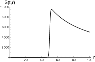
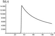
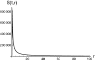
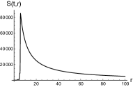
Figure 2: Plots of the surface gravity function, $S(t,r)$, at four different times. Top left plot is close to the initial time, top right at an intermediate time, bottom left at a time very close to when $S(t,r)$ attains its maximum value, and bottom right after the maximum has been attained. Note that the maximum value of $S(t,r)$ in the bottom left plot is $\sim 800,000$, while the peak values in the other three plots are at $\sim 8000$, $14000$ and $80,000$.

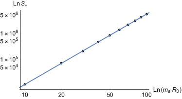
Figure 3: Log-log plot (dots) of the numerically evaluated maximum surface gravity of the collapsing spherical wall versus initial radius of the wall. The straight line fit shown is $\ln(S_{*})=3.08805+2.69554\ln(m_{a}R_{0})$.

The typical black hole mass at formation is given by the energy in a horizon size membrane. Using Eq. (10) we get,

$$M(t_{a})=\sigma\pi t_{a}^{2}\approx 2\times 10^{-8}~{}{\rm M}_{\odot}~{}f_{*}$$ (19)

where $1\,{\rm M}_{\odot}\approx 2\times 10^{33}\,{\rm gms}$. For comparison, the mass of the Earth is $\approx 3\times 10^{-6}~{}{\rm M}_{\odot}$ and the mass of the Moon is $\approx 4\times 10^{-8}~{}{\rm M}_{\odot}$.

The growth of primordial black holes has been of long-standing interest and has recently been discussed in Refs. Guedens et al. (2002); Deng et al. (2017). A basic picture of the growth is given by

$${\dot{M}}=\rho A$$ (20)

where $\rho$ is the ambient radiation energy density and $A$ is the area of the black hole: $A=4\pi R^{2}=16\pi G^{2}M^{2}$. The differential equation (20) can be solved and the growth of the black hole is determined by the ratio of its mass to the energy within the horizon at $t_{a}$,

$$\frac{M(t_{a})}{M_{H}(t_{a})}\sim 10^{-8}.$$ (21)

As this fraction is very small, the growth is negligible and can be ignored, giving

$$M(t_{0})\approx 2\times 10^{-8}\,{\rm M}_{\odot}~{}f_{*}.$$ (22)

The Schwarzschild radius of one of these black holes is $R_{S}\approx 6\times 10^{-8}~{}{\rm km}~{}f_{*}\sim 0.1~{}{\rm mm}~{}f_{*}$.

The number density of black holes depends on how many membranes undergo gravitational collapse. Not every membrane will be sufficiently symmetric, and angular momentum can prevent the membrane from contracting to its Schwarzschild radius. There is also a chance that a convoluted collapsing membrane will fragment further, however this requires a self-intersection along an entire closed curve. (A generic self-intersection will occur at two points and that will change the topology of the wall without leading to fragmentation.) Let us denote by $p_{\rm bh}$ the probability that a large membrane, for which radiative losses can be ignored, collapses to a black hole. So $p_{\rm bh}$ absorbs our ignorance of the membrane angular momentum and fragmentation probability.

In terms of $p_{\rm bh}$ the mass density in black holes at time $t_{a}$ is

$$\rho_{\rm bh}(t_{a})\sim\frac{p_{\rm bh}\,M(t_{a})}{4\pi t_{a}^{3}/3}$$ (23)

and their energy density relative to the critical density, $\rho_{c}=3/(32\pi Gt^{2})$, at formation is

$$\Omega_{\rm bh}(t_{a})=\frac{\rho_{\rm bh}(t_{a})}{\rho_{c}(t_{a})}\approx 2\times 10^{-8}p_{\rm bh}~{}f_{*}.$$ (24)

The relative energy density grows with scale factor in the radiation era and at the present epoch is

$$\Omega_{\rm bh}(t_{0})=\Omega_{\rm bh}(t_{a})\left(\frac{T_{a}}{T_{\rm eq}}\right)\approx 2\,p_{\rm bh}\,f_{*}$$ (25)

where $T_{\rm eq}\approx 1~{}{\rm eV}$ is the temperature at the epoch of matter-radiation equality.

Estimates have been made for black hole formation probability from cosmic string loops Hawking (1989); Polnarev and Zembowicz (1991). A general argument proposed by Rees (reviewed in Vilenkin and Shellard (2000)) is based on the angular momentum barrier to gravitational collapse – a string loop can only collapse to a black hole of mass $M$ if its angular momentum is less than the maximum allowed for a black hole, $J_{\rm max}=GM^{2}$. In the case of global strings, we expect the strings to be less curved than local strings, and the membranes to be relatively flat, as also seen in simulations (see Fig. 2 of Hiramatsu et al. (2012)). We will assume that a membrane inherits all its angular momentum from the motion of strings that intersect. Since the strings move at relativistic velocities and have size $R_{0}$, the angular momentum of a membrane is $J\sim\mu R_{0}^{2}$.

$$\frac{J_{\rm max}}{J}\sim\frac{GM^{2}}{\mu R_{0}^{2}}\sim 4\times 10^{-3}.$$ (26)

First following Rees, we assume that every component of the angular momentum is independent and uniformly distributed, and we require that all components be smaller than $J_{\rm max}$. Then we estimate

$$p_{\rm bh}\sim\left(\frac{J_{\rm max}}{J}\right)^{3}\sim 10^{-7}$$ (27)

which gives $\Omega_{\rm bh}(t_{0})\sim 10^{-7}f_{*}$.

On the other hand, we do not expect all three components of the angular momentum to be independent. The velocity of a string has to be perpendicular to the tangent direction to the string. So if a membrane is formed from the intersection of two relatively straight strings, we expect that the angular momentum vector component along the strings will be large but the components in the orthogonal directions will be small. In this case a more suitable upper bound is

$$p_{\rm bh}\sim\frac{J_{\rm max}}{J}\sim 2\times 10^{-3}$$ (28)

which gives $\Omega_{\rm bh}(t_{0})\sim 4\times 10^{-3}\,f_{*}$.

Clearly these are tentative estimates of $p_{\rm bh}$ and need to be investigated more carefully. However, it is likely that $\Omega_{\rm bh}(t_{0})$ is much smaller than 1 and will not violate microlensing constraints which give $\Omega_{\rm bh}(t_{0})\lesssim 0.01$ (see Fig. 20 of Niikura et al. (2017)). If our estimates of $p_{\rm bh}$ are too conservative and $\Omega_{\rm bh}(t_{0})\sim 0.01$ then these black holes may be a significant component of the cosmic dark matter Bird et al. (2016) in addition to the usual coherent axionic dark matter.

The mass spectrum of black holes will be determined by the mass distribution of membranes once the string-wall network fragments. Drawing an analogy with the better studied monopole-string systems in which the length distribution of strings is exponentially suppressed Vilenkin and Shellard (2000), we expect that the mass spectrum of membranes will be exponentially suppressed by the initial area of the membrane. Then the resulting black hole mass spectrum will also be exponentially suppressed by the mass of the black hole and only the lowest mass black holes will be relevant. Further, the recent analysis in Ref. Bird et al. (2016) for the black hole merger rate within galaxy halos will apply to axion black holes as well. The analysis assumes a dark matter density for the black holes but the resulting merger rate is independent of the black hole mass.

With the parameters of the QCD axion the black hole masses are too small by a factor of $\sim 10^{9}$ to be the black holes seen by LIGO. If we consider an “axion-like particle” (ALP) instead of the QCD axion, and if the physics of the ALP also leads to a string-wall network that fragments, the resulting black holes could have significantly higher masses. It would be worth examining black hole formation in a concrete ALP model.