Confined Sandpile in two Dimensions: Percolation and Singular Diffusion

Abstract

We investigate the properties of a two-state sandpile model subjected to a confining potential in two dimensions. From the microdynamical description, we derive a diffusion equation, and find a stationary solution for the case of a parabolic confining potential. By studying the systems at different confining conditions, we observe two scale-invariant regimes. At a given confining potential strength, the cluster size distribution takes the form of a power law. This regime corresponds to the situation in which the density at the center of the system approaches the critical percolation threshold. The analysis of the fractal dimension of the largest cluster frontier provides evidence that this regime is reminiscent of gradient percolation. By increasing further the confining potential, most of the particles coalesce in a giant cluster, and we observe a regime where the jump size distribution takes the form of a power law. The onset of this second regime is signaled by a maximum in the fluctuation of energy.

I Introduction

Anomalous diffusion is observed in many physical scenarios such as fluid transport in porous media Kuntz2001 ; Lukyanov2012 , diffusion in crowded fluids Szymanski2009 , diffusion in fractal-like substrates Stephenson1995 ; Andrade1997 ; Buldyrev2001 ; Costa2003 ; Havlin2002 , turbulent diffusion in the atmosphere Richardson1926 ; Hentschel1984 , diffusion of proteins due to molecular crowding Banks2005 , systems including ultra-cold atoms Sagi2012 , analysis of heartbeat histograms Grigolini2001 , diffusion in “living polymers” Ott1990 and study of financial transactions Plerou2000 . Anomalous diffusion can also manifest its non-Gaussian behavior in terms of nonlinear Fokker-Plank equations Lenzi2001 ; Malacarne2001 ; Malacarne2002 ; DaSilva2004 ; Lenzi2005 , which is the case, for example, of the dynamics of interacting vortices in disordered superconductors Zapperi2001 ; Moreira2002 ; Miguel2003 ; Andrade2010 , diffusion in dusty plasma Liu2008 ; Barrozo2009 , and pedestrian motion Barrozo2009 . A very interesting case of anomalous diffusion is surely the singular diffusion which is identified as having a divergent diffusion coefficient Carlson1990 ; Carlson1993 ; Carlson1995 ; Kadanoff1992 ; Barbu2010 . This kind of behavior happens in nature in some physical situations, for instance when adsorbates diffuse on a adsorbent surface, its diffusion can be very nonlinear with a diffusion coefficient which depends on the local coverage $\theta$ as, $D\propto{\left|\theta-\theta_{c}\right|^{-\alpha}}$ Myshlyavtsev1995 . Therefore, the study of the basic mechanisms behind surface diffusion is of large importance for understanding technologically important processes like physical adsorption Vidali1991 and catalytic surface reactions Manandhar2003 ; Hofmann2005 ; Schmidtbauer2012 .

A special class of singular diffusion models were intensively studied by Carlson et al. Carlson1990 ; Carlson1993 in two state 1D sandpile models for which they derive diffusion equations with singularities in the diffusion coefficient of the form $D\propto(1+\rho)/(1-\rho)^{3}$, where $\rho$ is the local density. They suggest that some open driven systems present self-organized criticality Bak1987 because in their continuum limit singularities appear in the diffusion constant at a critical point Carlson1990 . Some characteristics of this model change drastically when a confining potential is applied Pires2015 . The jump-size distribution, for instance, starts to exhibit a power-law behavior which suggests a scale-invariant behavior of the system Pires2015 . Scale-invariant behavior in diffusive systems were also observed in gradient percolation diffusion fronts in 2D Sapoval1985 , that have been shown to display fractal diffusion fronts with characteristic dimension similar to the boundary of critical percolation clusters Sapoval1985 .

In this paper we investigate a 2D confined sandpile model. Our model is the extension of the model introduced in Pires2015 to the case of two dimensions. We are able to deduce the continuous limit for the model, which culminate in a diffusion equation with a singular diffusion coefficient. We observe in the confined system the onset of two scale invariant regimes. The first one occurs when the concentration at the origin (the center of the confining region) reaches the critical percolation threshold. At this point we observe scale invariance in the cluster size distribution as well as fractality in the perimeter of the central cluster. At more confined regimes, when the concentration reaches the critical threshold of singular diffusion, there is another signature of scale invariance in the jump size distribution.

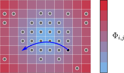
Figure 1: Schematic picture of the 2D confined sandpile model. The sites with discs inside are occupied, the site with a black disc inside is the source site of the jump, and the arrow points to the target site of the jump. The jump is the colored arrow. The tone gradient indicates the local potential $\Phi$.

II Model Formulation

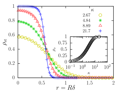
Figure 2: Occupation density as function of $r$ for different values of $\kappa$. The points are estimated from a radial histogram of the occupation averaged over time with $N_{p}=8000$ particles, while the solid lines are the predictions of Eq.(7). The inset shows the occupation density calculated at $r=0$. The solid line is the analytical prediction $\rho_{o}=1-\exp(-\beta\kappa{N}_{p}\delta^{2}/\pi)$.

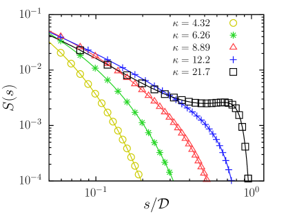
Figure 3: Jump size distribution for different values of $\kappa$ with $N_{p}=8000$. The points are numerical simulations and the solid lines are the predictions of Eq. (8). Here we define $\mathcal{D}=2\sqrt{N_{p}/\pi}$ as the diameter of a dense disc with $N_{p}$ particles.

In the present model, $N_{p}$ particles are placed on a square lattice where we define the occupation $h_{i,j}$ for each site as $0$ (if the site is empty) or $1$ (if the site is occupied). As shown in Fig. 1, at each iteration, a particle can move randomly to any of four directions of the square lattice. The particle moves from an occupied site (the source) and get past all occupied sites on the chosen direction until it reaches an empty site (the target) where it may stay with a given probability (see Fig. 1) in a movement that we label a jump. The probability that a jump is accepted is given by the Metropolis factor $\Theta=\min(1,\exp(-\beta[\Phi_{i_{t},j_{t}}-\Phi_{i_{s},j_{s}}]))$, where we define $\Phi_{i,j}$ as the external potential energy of a site. This probability introduces the effect of a confining potential on the particles. Here we present result using only four directions, since, for this case, a continuous limit of the model can be found analytically. However we also performed simulations with a model where particles can move in any arbitrary direction, leading to entirely similar results.

III Continuous limit of the model

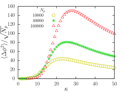
Figure 4: Mean jump energy fluctuation as function of $\kappa$ for different number of particles $N_{p}$. The points are the results from Eq. 9. For each value of $N_{p}$, the energy fluctuation exhibits a maximum at a different value $\kappa^{*}(N_{p})$.

It is possible to verify that the model we described is a Markov process, that is, the occupation probability of a site $(i,j)$ at a given step $n+1$, $\rho_{i,j|n+1}$, can be obtained from the occupation probability of all sites on the previous step,

$$\rho_{i,j|n+1} = \rho_{i,j|n}$$ (1)

$$+ \sum_{i^{\prime}\neq i}\frac{1}{4}P_{i,i^{\prime}-1|j}\rho_{i^{\prime},j|n}(1-\rho_{i,j|n})\Theta_{i,i^{\prime}|j}$$

$$- \sum_{i^{\prime}\neq i}\frac{1}{4}P_{i,i^{\prime}-1|j}\rho_{i,j|n}(1-\rho_{i^{\prime},j|n})\Theta_{i^{\prime},i|j}$$

$$+ \sum_{j^{\prime}\neq j}\frac{1}{4}P_{i|j,j^{\prime}-1}\rho_{i,j|n}(1-\rho_{i,j|n})\Theta_{i|j,j^{\prime}}$$

$$- \sum_{j^{\prime}\neq j}\frac{1}{4}P_{i|j,j^{\prime}-1}\rho_{i,j|n}(1-\rho_{i,j^{\prime}|n})\Theta_{i|j^{\prime},j},$$

where $\Theta_{i|j,j^{\prime}}=\min(1,\exp(-\beta[\Phi_{i,j}-\Phi_{i,j^{\prime}}]))$ is the Metropolis factor, and $P_{i|j,j^{\prime}}$ is the probability of finding all sites between $j$ and $j^{\prime}$ in the $i$ column occupied. Similarly, $\Theta_{i,i^{\prime}|j}=\min(1,\exp(-\beta[\Phi_{i,j}-\Phi_{i^{\prime},j}]))$, where $P_{i,i^{\prime}|j}$ is the probability of finding all sites between column $i$ and $i^{\prime}$ on the $j$ line occupied. We define the probabilities of finding $k$ consecutive sites occupied in a given direction as

$$\Omega^{\pm}_{i,j|k}=\prod_{k^{\prime}=1}^{k}\rho_{i\pm k^{\prime},j}\quad\text{and}\quad\Psi^{\pm}_{i,j|k}=\prod_{k^{\prime}=1}^{k}\rho_{i,j\pm k^{\prime}},$$

where $\Omega^{\pm}_{i,j|k}$ is used for the horizontal direction and $\Psi^{\pm}_{i,j|k}$ is used for the vertical direction. We then define,

$$\Xi^{\pm}_{i,j}=\sum_{i^{\prime}=1}^{\infty}\Theta_{i,i\pm i^{\prime}|j}\Omega^{\pm}_{i,j|i^{\prime}}$$

as the contribution for the probability due to particles arriving from the horizontal direction. In a similar fashion, we define $\Gamma^{\pm}_{i,j}$ as the contribution due to particles arriving from vertical direction, and

$$\Lambda^{\pm}_{i,j}=\sum_{i^{\prime}=1}^{\infty}(1-\rho_{i\pm i^{\prime},j})\Theta_{i\pm i^{\prime},i|j}\Omega^{\pm}_{i,j|i^{\prime}-1}$$

as the contribution due to particles leaving in the horizontal direction. Finally, $\Upsilon^{\pm}_{i,j}$ is the contribution due to particles leaving in vertical direction.

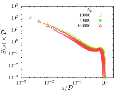
Figure 5: Jump size distribution for $\kappa=\kappa^{*}$ and different values of $N_{p}$. This result is obtained through Eq. 8 choosing $S_{o}$ in such a way that $S(s)$ is normalized. The factor $\mathcal{D}=2\sqrt{N_{p}/\pi}$ is the diameter of a compact cluster with all particles.

Using these definitions, Eq. (1) can be written as

$$\frac{\rho_{i,j|n+1}-\rho_{i,j|n}}{\tau} = \frac{(1-\rho_{i,j})}{4\tau}(\Xi^{+}_{i,j}+\Xi^{-}_{i,j}+\Gamma^{+}_{i,j}+\Gamma^{-}_{i,j})$$ (2)

$$- \frac{\rho_{i,j}}{4\tau}(\Lambda^{+}_{i,j}+\Lambda^{-}_{i,j}+\Upsilon^{+}_{i,j}+\Upsilon^{-}_{i,j}),$$

where $\tau$ is the time unit. The first factor on the right side of Eq. (2) accounts for particles arriving at a given site from each of four directions of the lattice, while the second factor on the left side of Eq. (2) accounts for particles leaving this site in each of the four directions of the lattice.

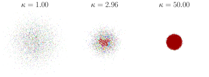
Figure 6: Snapshots of simulations of systems with 10000 particles for different value of $\kappa$. The colors indicate different clusters. Observe the relative size of the clusters and the formation of a giant cluster when $\kappa$ increases.

The continuous limit of Eq. (2) can be obtained similarly to what was done for 1D Pires2015 , resulting in the following non-linear diffusion equation

$$\frac{\partial\rho}{\partial t}=D\nabla\cdot\left[\frac{(1+\rho)}{(1-\rho)^{3}}\nabla\rho+\beta\frac{(1+\rho)}{(1-\rho)^{2}}\rho\nabla\Phi\right],$$ (3)

where we define

$$D=\mathop{\lim_{\mathop{\delta\rightarrow 0}}}_{\tau\rightarrow 0}\frac{\delta^{2}}{4\tau},$$ (4)

with $\delta$ been the space unit used for the space continuous limit and $\rho=\rho(x=i\delta,y=j\delta,t=n\tau)$. From Eq. 3, we see that our model obeys the continuity equation $\partial\rho/\partial t=-\nabla\mathbf{J}$, where we have

$$\mathbf{J}=-D\left[\frac{(1+\rho)}{(1-\rho)^{3}}\nabla\rho+\beta\frac{(1+\rho)}{(1-\rho)^{2}}\rho\nabla\Phi\right].$$

In the case where the dependence of the potential is only radial, $\Phi=\Phi(r)$, the conditions for a stationary solution are $\partial\Phi/\partial r=0$, $\rho_{\text{st}}(r\rightarrow\infty)\rightarrow 0$ and $\mathbf{J}=\mathbf{0}$. Thus,

$$r\left[\frac{(1+\rho)}{(1-\rho)^{3}}\frac{d\rho}{dr}+\beta\frac{(1+\rho)}{(1-\rho)^{2}}\rho\frac{d\Phi}{dr}\right]=0.$$

which can be written as

$$\frac{1}{\beta(1-\rho)\rho}\frac{d\rho_{\text{st}}}{dr}=-\frac{d\Phi}{dr}=\frac{d}{dr}\left[\int_{u_{0}}^{\rho_{\text{st}}}\frac{1}{\beta(1-u)u}du\right].$$ (5)

The Eq. (5) can be easily solved and results in the stationary solution given by

$$\rho_{\text{st}}(r)=\frac{1}{1+e^{\beta[\Phi(r)-\mu]}},$$ (6)

where $\mu$ can be obtained from the constraint $\int\frac{\rho(r)}{\delta^{2}}dS=N_{p}$, leading to

$$\int_{0}^{\infty}\frac{1}{1+e^{\beta[\Phi(r)-\mu]}}rdr=\frac{N_{p}\delta^{2}}{2\pi}.$$

In the particular case of a parabolic confining potential, $\Phi(r=R\delta)=\kappa r^{2}=\kappa(i^{2}+j^{2})\delta^{2}$, this integral can be solved, and it is possible to show that $\mu=(1/\beta)\ln(\exp(\beta\kappa N_{p}\delta^{2}/\pi)-1)$, so that Eq. (6) is now independent of $\mu$

$$\rho_{\text{st}}(r)=\frac{(e^{\beta\frac{\kappa N_{p}\delta^{2}}{\pi}}-1)}{e^{\beta\frac{\kappa N_{p}\delta^{2}}{\pi}}+(e^{\beta\kappa r^{2}}-1)}.$$ (7)

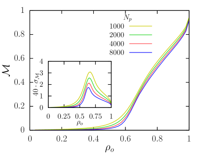
Figure 7: Fraction of the largest cluster $\mathcal{M}$ computed from numerical simulations as function of occupation density at the origin $\rho_{o}$ for different values of number of particles $N_{p}$. The inset shows the standard deviation of $\mathcal{M}$ as function of $\rho_{o}$.

In Fig. 2, we can see the agreement between predictions from Eq. (7) and results from numerical simulations. Due to the intrinsic exclusion mechanism of the model, the stationary state given by Eq. (6) is a Fermi-Dirac distribution Fernando2010 , and as $\kappa$ increases, the occupation tends to saturate at $\rho_{\text{st}}=1$ near $r=0$. This behavior leads to the formation of a giant cluster of particles near the origin as $\kappa$ increases. The occupation at $r=0$ follows $\rho_{o}=1-\exp(-\beta\kappa N_{p}\delta^{2}/\pi)$, and, as the inset in Fig. 2 shows, this prediction follows closely the results from numerical simulations.

IV Jump Size Distribution and Mean Square Energy Fluctuation

At this point, it is important to define a quantity that can give information about the dynamics of the model, which is the jump size distribution

$$S(s)\approx\lim_{t\rightarrow\infty}\left[\frac{\mathcal{N}_{[t]}(s)}{\mathcal{N}_{[t]T}}\right],$$

where $s$ is the size of a jump, $S(s)$ is the probability of a jump of size $s$ to occur, $\mathcal{N}_{[t]}(s)$ is the number of jumps of size $s$ that appeared in a time interval $t$, and $\mathcal{N}_{[t]T}$ is the total number of jumps in a time interval. Assuming that it is possible to obtain the dynamics of the model from the occupation probability, we can use the following approximation:

$$S(s)\equiv S_{o}\sum_{i}\sum_{j}\frac{{\rho}_{i,j}}{4}\left[\lambda^{+}_{i,j|s}+\lambda^{-}_{i,j|s}+\upsilon^{+}_{i,j|s}+\upsilon^{-}_{i,j|s}\right],$$ (8)

where $S_{o}$ is a normalization constant, and we obtain the occupation probability from the stationary condition, $\rho_{i,j}=\rho_{st}(x=i\delta,y=j\delta)$. The factors $\lambda^{\pm}_{i,j|s}$ account for the chance of a jump to be accepted in the horizontal direction and is defined as

$$\lambda^{\pm}_{i,j|s}=(1-\rho_{i\pm s,j})\Theta_{i\pm s,i|j}{\Omega}^{\pm}_{i,j|s-1}.$$

Similarly, $\upsilon^{\pm}_{i,j|s}$ accounts for the chance of a jump being accepted in the vertical direction and is defined in a similar fashion. We performed the summations of Eq.(8) numerically and compared it with the results from numerical simulations. The results are displayed in Fig. 3, showing very good agreement.

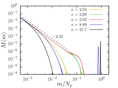
Figure 8: Cluster size distribution obtained through numerical simulations for $N_{p}=8000$ and different values of $\kappa$. The dashed line is a power law with exponent equal to $-2.35$.

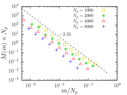
Figure 9: Log-log plot of the cluster size distribution obtained through numerical simulations for different values of $N_{p}$ and $\kappa=\kappa^{\prime}$. The dashed line is a power law with exponent equal to $-2.35$.

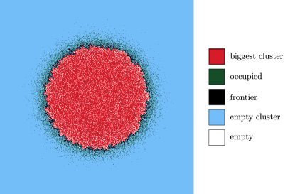
Figure 10: Diffusion frontier with $N_{p}=100000$ and $\kappa=20.0$. This picture shows the results of a simulation on a 2D square lattice were we put $100000$ particles following the probability given by Eq. (7). The red sites are the occupied sites that belong to the largest cluster and the black are the largest cluster sites that belong to the diffusion frontier. The gray sites are the occupied sites that do not belong to the largest cluster. The white sites are empty, and the blue ones correspond to the empty sites that belong to the empty cluster (connected through first or second neighbors to the more external empty sites). In this picture, there are 5960 sites at the diffusion frontier.

As $\kappa$ increases, the occupation at the center of the system saturates to one (see Fig. 2). Consequently, in very confined systems, jumps that pass through the whole system have larger probability, as indicated by the peak at a large value of $s$ in Fig. 3 when $\kappa=21.7$. The agreement between numerical simulations and the predictions from Eq. (8) shown in Fig. 3 allow us to confidently study larger systems and extract useful information without the need to run time expensive simulations.

Another useful information about the dynamics of the model is the mean square energy fluctuation of the system, which can be determined from the probabilities $\lambda^{+}_{i,j|s}$ and $\upsilon^{+}_{i,j|s}$ as,

$$\langle\Delta\phi^{2}\rangle \equiv \sum_{s}\sum_{i}\sum_{j}\frac{\rho_{i,j}}{4}\left[\lambda^{+}_{i,j|s}(\Phi_{i,j+s}-\Phi_{i,j})^{2}\right.$$ (9)

$$+ \lambda^{-}_{i,j|s}(\Phi_{i,j-s}-\Phi_{i,j})^{2}+\upsilon^{+}_{i,j|s}(\Phi_{i+s,j}-\Phi_{i,j})^{2}$$

$$+ \left.\upsilon^{-}_{i,j|s}(\Phi_{i-s,j}-\Phi_{i,j})^{2}\right].$$

where the sum goes over all jump sizes $s$ and all sites $(i,j)$. Figure 4 shows the $\langle\Delta\phi^{2}\rangle$ as function of $\kappa$ for different number of particles. As can be seen, this function have a maximum in a specific value of $\kappa^{*}$ for each value of $N_{p}$. The shape of the jump size distribution at the condition of maximum energy fluctuation appears to be size invariant, as shown in Fig. 5. The distributions in Fig. 5 collapse when the jump size is scaled by the diameter $\mathcal{D}=2\sqrt{N_{p}/\pi}$ of a dense cluster with all particles. This result is suggestive of a scale invariant regime observed at $\kappa=\kappa^{*}$.

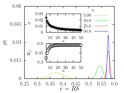
Figure 11: Probability of finding a diffusion frontier site at a distance $r$. In the inset, we show $\sigma$, the standard deviation of the distance of the diffusion frontier sites to origin, and $\mathcal{R}_{f}$, the diffusion frontier radius as function of the strength $\kappa$ of the confining potential. Here we used $N_{p}=10000000$.

V Cluster Size Distribution and Diffusion Frontier

In this section we investigate some of the geometric aspects of our model. Figure 6 shows the formation of a giant cluster centered at the origin of the confining potential, as the strength $\kappa$ increases. As $\kappa$ grows, there is a clear percolation-like behavior induced where the large cluster starts to grow at the origin. This can be observed quantitatively by investigating the mean largest cluster size $\mathcal{M}$ which can be obtained at each time step. Figure 7 shows how the mean largest cluster size changes when $\kappa$ increases. For convenience, we plot $\mathcal{M}$ as a function of the density at the origin $\rho_{o}$, which increases monotonically with $\kappa$, (see the inset of Fig. 2). As depicted, there is a sudden increase in the size of the largest cluster for $\rho_{o}\approx p_{c}$, where $p_{c}=0.59274621(13)$ is the percolation critical point Newman2000 . Figure 8 suggests that this increasing in the size of the largest cluster takes place due to a percolation-like transition that changes the cluster size distribution of this model. This conjecture may be supported by investigating the cluster size distribution at the condition where the confining potential starts to induce the formation of a larger cluster in the center of the system, $\kappa^{\prime}=\kappa(\rho_{o}=p_{c})\approx 2.82$. Figure 9 shows that the cluster size distribution at this value of $\kappa$ follows a power law.

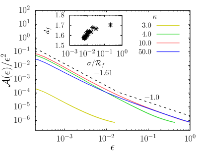
Figure 12: Fractal dimension determination from multiple resolution analysis. The slope of the dashed line is $-d_{f}$ according to Eq. 10. The dashed line represents approximately the slope for most curves analyzed. The inset shows us how $d_{f}$ grows with $\sigma/\mathcal{R}_{f}$.

Another relevant quantity that can be considered is the cluster external perimeter (the so called hull) of the largest cluster. As shown in Fig. 10, this structure is what we call the diffusion frontier and its characteristics are closely related to the gradient percolation diffusion front Sapoval1985 . We define the frontier radius $\mathcal{R}_{f}$ as the mean distance of the diffusion frontier sites to the origin. To study systems with a lager number of particles, we used random samples Knuth1981 to generate a sample system from Eq. 7. Figure 11 shows the probability of finding a diffusion frontier site at a given distance to the origin. The insets in the Fig. 11 shows $\sigma$, the standard deviation of the distance of the diffusion frontier sites to origin, and $\mathcal{R}_{f}$, the diffusion frontier radius as a function of the strength $\kappa$ of the confining potential. One important difference between our model and usual gradient percolation models is the relation between the linear size $\mathcal{R}_{f}$ and $\sigma$, since both are function of $\kappa$, in such way that we cannot fix one and vary the other. This condition limits the values of $\mathcal{R}_{f}$ and $\sigma$ that are close to the condition where finite size effects affect the diffusion frontier. In Fig. 12, we use multiple resolution analysis Peleg1984 ; Peli1990 to estimate the fractal dimension $d_{f}$ of the diffusion frontier. This method consists in considering all points at a distance less than a given $\epsilon$ from the set for which the fractal dimension is being estimated. These points form a new set with the area given by the Richardson law Peli1990

$$\mathcal{A}(\epsilon)\propto\epsilon^{2-d_{f}}.$$ (10)

One can see, at higher scales, that the frontier appears as a one dimensional line, crossing over to a higher fractal dimension $d_{f}$ at smaller scales. As $\kappa$ decreases, approaching the value $\kappa^{\prime}$ where $\rho_{0}\approx p_{c}$, the values of the higher dimension $d_{f}$ grows, but the scaling region decreases. In the inset of Fig. 12, we can see how $d_{f}$ changes with $\sigma/\mathcal{R}_{f}$.

VI Conclusions

We studied a 2D two-state confined sandpile model. From a microscopic dynamics we derived a singular diffusion equation and were able to obtain an analytical stationary solution for the particular case of parabolic potential. This system appears to display two scale-invariant regimes. The first is observed when the concentration at the origin approaches the critical value for percolation. This regime is similar to what is observed for gradient percolation, that is, power laws in the cluster size distribution are observed, as well as a fractal shape for the singular diffusion frontier. The second regime is associated with more intense confinements, when the concentration in the center approaches the maximum value, and a scale-invariant behavior is observed for the jump size distribution. We derived an analytical expression for the jump size distribution and find it to be in good agreement with our numerical solutions. We could, also, find a natural way to define the onset of the scale-invariant regime as the situation where the energy fluctuations are maximum.

VII Acknowledgments

We thank the Brazilian agencies CNPq, CAPES, FUNCAP, and the National Institute of Science and Technology for Complex Systems (INCT-SC) in Brazil for financial support.

References

- (1) M. Küntz and P. Lavallée, J. Phys. D: Appl. Phys. 34, 2547–2554 (2001).
- (2) A. V. Lukyanov, M. M. Sushchikh, M. J. Baines and T. G. Theofanous, Phys. Rev. Lett. 109, 214501 (2012).
- (3) J. Szymanski and M. Weiss, Phys. Rev. Lett. 103, 038102 (2009).
- (4) J. Stephenson, Physica A 222, 234–247 (1995).
- (5) J. S. Andrade Jr., D. A. Street, Y. Shibusa, S. Havlin and H. E. Stanley, Phys. Rev. E 55, 772–777 (1997).
- (6) S. V. Buldyrev, S. Havlin, A. Y. Kazakov, M. G. E. da Luz, E. P. Raposo, H. E. Stanley and G. M. Viswanathan, Phys. Rev. E 64, 041108 (2001).
- (7) M. H. A. S. Costa, A. D. Araújo, H. F. da Silva. and J. S. Andrade Jr., Phys. Rev. E 67, 061406 (2003).
- (8) S. Havlin and D. Ben-Avraham, Adv. Phys. 51, 187–292 (2002).
- (9) L. F. Richardson, P. Roy. Soc. Lond. A Mat. 110, 709–737 (1926).
- (10) H. G. E. Hentschel and I. Procaccia, Phys. Rev. A 29, 1461–1470 (1984).
- (11) D. S. Banks and C. Fradin, Biophys. J. 89, 2960–2971 (2005).
- (12) Y. Sagi, M. Brook, I. Almog and N. Davidson, Phys. Rev. Lett. 108, 093002 (2012).
- (13) P. Grigolini, L. Palatella and G. Raffaelli, Fractals 9, 349–449 (2001).
- (14) A. Ott, J. P. Bouchaud, D. Langevin and W. Urbach, Phys. Rev. Lett. 65, 2201–2204 (1990).
- (15) V. Plerou, P. Gopikrishnan, L. A. N. Amaral, X. Gabaix and H. E. Stanley, Phys. Rev. E 62, R3023–R3026 (2000).
- (16) E. K. Lenzi, C. Anteneodo and L. Borland, Phys. Rev. E 63, 051109 (2001).
- (17) L. C. Malacarne, R. S. Mendes, I. T. Pedron and E. K. Lenzi, Phys. Rev. E 63, 030101 (2001).
- (18) L. C. Malacarne, R. S. Mendes, I. T. Pedron and E. K. Lenzi, Phys. Rev. E 65, 052101 (2002).
- (19) P. C. da Silva, L. R. da Silva, E. K. Lenzi, R. S. Mendes and L. C. Malacarne, Physica A 342, 16–21 (2004).
- (20) E. K. Lenzi, R. S. Mendes, J. S. Andrade Jr., L. R. da Silva and L. S. Lucena, Phys. Rev. E 71, 052101 (2005).
- (21) S. Zapperi, A. A. Moreira and J. S. Andrade Jr., Phys. Rev. Lett. 86, 3622–3625 (2001).
- (22) A. A. Moreira, J. S. Andrade Jr., J. Mendes Filho and S. Zapperi, Phys. Rev. B 66, 174507 (2002).
- (23) M. Migel, J. S. Andrade Jr. and S. Zapperi, Braz. J. Phys. 33, 557–572 (2003).
- (24) J. S. Andrade Jr., G. F. T. da Silva, A. A. Moreira, F. D. Nobre and E. M. F. Curado, Phys. Rev. Lett. 105, 260601 (2010).
- (25) B. Liu and J. Goree, Phys. Rev. Lett. 100, 055003 (2008).
- (26) P. Barrozo, A. A. Moreira, J. A. Aguiar and J. S. Andrade Jr., Phys. Rev. B 80, 104513 (2009).
- (27) J. M. Carlson, J. T. Chayes, E. R. Grannan and G. H. Swindle, Phys. Rev. Lett. 65, 2547–2550 (1990).
- (28) J. M. Carlson, E. R. Grannan, C. Singh and G. H. Swindle, Phys. Rev. E 48, 688–698 (1993).
- (29) J. M. Carlson and G. H. Swindle, Proc. Natl. Acad. Sci. USA 92, 6712–6719 (1995).
- (30) L. P. Kadanoff, A. B. Chhabra, A. J. Kolan, M. J. Feigenbaum and I. Procaccia, Phys. Rev. A 45, 6095–6098 (1992).
- (31) V. Bardu, Annu. Rev. Control 34, 52–61 (2010).
- (32) A. V. Myshlyavtsev, A. A. Stepanov, C. Uebing and V. P. Zhdanov, Phys. Rev. B 52, 5977–5984 (1995).
- (33) G. Vidali, G. Ihm, H. Kim and M. W. Cole, Surf. Sci. Rep. 12, 133–181 (1991).
- (34) P. Manandhar, J. Jang, G. C. Schatz, M. A. Ratner and S. Hong, Phys. Rev. Lett. 90, 115505 (2003).
- (35) S. Hofmann, G. Csányi, A. C. Ferrari, M. C. Payne and J. Robertson, Phys. Rev. Lett. 95, 036101 (2005).
- (36) J. Schmidtbauer, R. Bansen, R. Heimburger, T. Teubner and T. Boeck, Appl. Phys. Lett. 101, 043105 (2012).
- (37) P. Bak, C. Tang and K. Wiesenfeld, Phys. Rev. Lett. 59, 381–384 (1987).
- (38) R. S. Pires, A. A. Moreira, H. A. Carmona and J. S. Andrade Jr., Europhys. Lett. 109, 14007 (2015).
- (39) B. Sapoval, M. Rosso and J. F. Gouyet, J. Physique Lett. 46, L149–L156 (1985).
- (40) A. E. Fernando, K. A. Landman and M. J. Simpson, Phys. Rev. E 81, 011903 (2010).
- (41) M. E. J. Newman and R. M. Ziff, Phys. Rev. Lett. 85, 4104 (2000).
- (42) D. E. Knuth, Seminumerical algorithms, Volume 2 of The art of computer programming. 2d ed. (Addison-Wesley, Massachusetts, 1981).
- (43) S. Peleg, J. Naor, R. Hartley and D. Avnir, IEEE T. Patern Anal. 6, 518–523 (1984).
- (44) E. Peli, J. Opt. Soc. Am. A 7, 2032–2040 (1990).