The strong coupling from a nonperturbative determination of
the $\Lambda$ parameter in three-flavor QCD

Abstract

We present a lattice determination of the $\Lambda$ parameter in three-flavor QCD and the strong coupling at the Z pole mass. Computing the nonperturbative running of the coupling in the range from $0.2\,{\rm GeV}$ to $70\,{\rm GeV}$, and using experimental input values for the masses and decay constants of the pion and the kaon, we obtain $\Lambda_{\overline{\rm MS}}^{(3)}=341(12)\,{\rm MeV}$. The nonperturbative running up to very high energies guarantees that systematic effects associated with perturbation theory are well under control. Using the four-loop prediction for $\Lambda_{\overline{\rm MS}}^{(5)}/\Lambda_{\overline{\rm MS}}^{(3)}$ yields $\alpha^{(5)}_{\overline{\rm MS}}(m_{\rm Z})=0.11852(84)$.

I Introduction

An essential input for theory predictions of high energy processes, in particular for phenomenology at the LHC Dittmaier et al. (2012); Andersen et al. (2013); Accardi et al. (2016); de Florian et al. (2016), is the QCD coupling $\alpha_{s}(\mu)=\bar{g}^{2}_{s}(\mu)/(4\pi)$ at energy scales $\mu\sim m_{\mathrm{Z}}$ and higher. In this work we present a sub-percent determination of the strong coupling at the Z pole mass using the masses and decay constants of the pion and kaon as experimental input and lattice QCD as computational tool.

Perturbation theory (PT) predicts the energy dependence of the coupling as

$$\bar{g}_{s}^{2}(\mu)\raisebox{-0.43057pt}{ $\stackrel{{\scriptstyle\small{\mu\to\infty}}}{{\sim}}$}\frac{1}{2b_{0}\log(\mu/\Lambda_{s})+(b_{1}/b_{0})\log\log(\mu/\Lambda_{s})}+\ldots$$ (1)

in terms of known positive coefficients, $b_{0,1}$, and a single parameter, $\Lambda_{s}$, which can also serve as the nonperturbative scale of the theory. The label $s$, called scheme, summarizes all details of the exact definition of $\bar{g}_{s}$. Conventionally one chooses the so-called $s={\rm\overline{MS\kern-0.50003pt}\kern 0.50003pt}$ scheme Bardeen et al. (1978), but $\Lambda$ parameters in different schemes can be exactly related with a one-loop computation Celmaster and Gonsalves (1979).

Our computation of $\alpha_{\rm\overline{MS\kern-0.35002pt}\kern 0.35002pt}$ is based on a determination of the three-flavor $\Lambda$ parameter. To outline the steps of our determination, we write

$$\Lambda^{(3)}_{\rm\overline{MS\kern-0.35002pt}\kern 0.35002pt}=\frac{\Lambda^{(3)}_{\rm\overline{MS\kern-0.35002pt}\kern 0.35002pt}}{\mu_{\rm PT}}\times\frac{\mu_{\rm PT}}{\mu_{\rm had}}\times\frac{\mu_{\rm had}}{f_{\pi\mathrm{K}}}\times f_{\pi\mathrm{K}}^{\rm PDG}\,.$$ (2)

As experimental input we use the PDG values Patrignani et al. (2016) for the following combination of decay constants

$$f_{\pi\mathrm{K}}\equiv\frac{1}{3}(2f_{\mathrm{K}}+f_{\pi})=147.6\,{\rm MeV}\,.$$ (3)

The key elements are then the determination of the ratio of scales $\mu_{\rm PT}/\mu_{\rm had}$ and the ratio $\mu_{\rm had}/f_{\pi\mathrm{K}}$, i.e., our hadronic scale in units of $f_{\pi\mathrm{K}}$. Both computations are performed in a fully nonperturbative way.

By choosing a large enough scale $\mu_{\rm PT}$ and including higher orders of PT in (1), the ratio $\Lambda^{(3)}_{\rm\overline{MS\kern-0.35002pt}\kern 0.35002pt}/\mu_{\rm PT}$ can be determined with negligible errors.

With $N_{\mathrm{f}}>2$ flavors, so far a single work Aoki et al. (2009) contains such a computation with all steps, including the connection of low energy $\mu_{\rm had}$ to large $\mu_{\rm PT}$, using numerical simulations and a step scaling strategy. This strategy, developed by the ALPHA collaboration Lüscher et al. (1991, 1994); de Divitiis et al. (1995); Jansen et al. (1996), supresses the systematic errors from the use of PT.

Here, we put together (and briefly review) the first factor in eq. (2) and our recent significant improvements in statistical and systematic precision in the second one Dalla Brida et al. (2016, 2017a), and finally add the missing third one.

QCD with $N_{\mathrm{f}}=3$ is the phenomenologically relevant effective theory at energies $E<m_{\mathrm{charm}}$ with small Bruno et al. (2015a); Korzec et al. (2017) corrections of order $(E/m_{\mathrm{charm}})^{2}$. However, for theory predictions of high energy processes, with $E\sim m_{\mathrm{Z}}$ and higher, the five- and six-flavor theories are needed. Fortunately, the ratios $\Lambda^{(N_{\mathrm{f}})}_{\rm\overline{MS\kern-0.35002pt}\kern 0.35002pt}/\Lambda^{(3)}_{\rm\overline{MS\kern-0.35002pt}\kern 0.35002pt},\;N_{\mathrm{f}}=4,5,6$ are known to very high order in PT, and successive order contributions decrease rapidly. This enables us to convert our $\Lambda^{(3)}_{\rm\overline{MS\kern-0.35002pt}\kern 0.35002pt}$ to precise values for $\alpha^{(5)}_{\rm\overline{MS\kern-0.35002pt}\kern 0.35002pt}(m_{\mathrm{Z}})$ and $\alpha^{(6)}_{\rm\overline{MS\kern-0.35002pt}\kern 0.35002pt}(1.508\,\mathrm{TeV})$, which can be used for high energy phenomenology. Further below, we will critically discuss the use of PT in this step.

II Strategy

Table 1: Summary of various scales used in this work.

Scale definition	purpose	$\mu/{\rm GeV}$
$\mu_{\rm PT}=16\,\mu_{0}$	matching with the asymptotic	$\approx 70$
	perturbative behavior
$\bar{g}_{\rm SF}^{2}(\mu_{0})=2.012$	nonperturbative matching	$\approx 4$
	between the GF and SF schemes
$\bar{g}_{\infty}^{2}(\mu_{\rm ref}^{\star})=1.6\pi^{2}$	setting scale in physical units	$\approx 0.5$
	by experimental value for $f_{\pi\mathrm{K}}$
$\bar{g}_{\rm GF}^{2}(\mu_{\rm had})=11.31$	matching between GF scheme	$\approx 0.2$
	and infinite-volume scheme

A nonperturbative definition of a coupling is easily given. Take a short-distance QCD observable, depending on fields concentrated within a 4-d region of Euclidean space of linear size $R=1/\mu$ and with a perturbative expansion

$${\cal O}_{s}(\mu)=k\,\bar{g}^{2}_{\rm\overline{MS\kern-0.35002pt}\kern 0.35002pt}(\mu)\,[1+c_{1}^{s}\bar{g}^{2}_{\rm\overline{MS\kern-0.35002pt}\kern 0.35002pt}(\mu)+\ldots]\,.$$ (4)

Then the nonperturbative coupling,

$$\bar{g}^{2}_{s}(\mu)\equiv{\cal O}_{s}(\mu)/k=\bar{g}^{2}_{\rm\overline{MS\kern-0.35002pt}\kern 0.35002pt}(\mu)+c_{1}^{s}\bar{g}^{4}_{\rm\overline{MS\kern-0.35002pt}\kern 0.35002pt}(\mu)+\ldots\,,$$ (5)

runs with $\mu$. This property also allows us to define scales $\mu$ by fixing $\bar{g}_{s}^{2}(\mu)$ to particular values (see Table 1). However, there is a challenge to reach the asymptotic region of small $\bar{g}_{s}^{2}(\mu)$, where eq. (1) is useful and its corrections can be controlled, using lattice simulations.

II.1 Challenge

Numerical computations involve both a discretization length, the lattice spacing $a$, and a total size of the system $L$, that is simulated. For standard observables, control over finite volume effects of order $\exp(-m_{\pi}L)$ requires $L$ to be several fm. At the same time, one needs to suppress discretization errors and should extrapolate $(a\mu)^{2}\to 0$ at fixed $\mu$. The necessary restrictions

$$L\gg 1/m_{\pi}\,,\quad 1/a\gg\mu\quad\Rightarrow\;L/a\ggg\mu/m_{\pi}$$ (6)

translate into very large lattices. Figure 1 displays the region in $\alpha(\mu)$ vs. $(a\mu)^{2}$ for the range $a\geq 0.04\,{\rm fm}$ which can be realized nowadays in large volumes ($m_{\pi}L\geq 4$). This shaded region is quite far from small coupling and small $(a\mu)^{2}$.

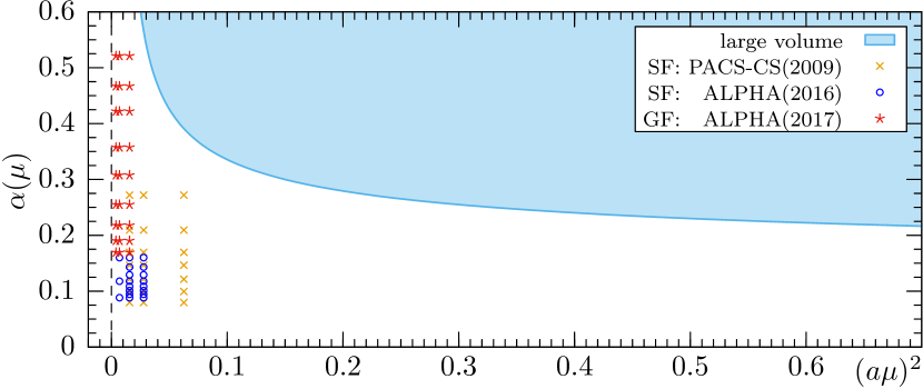
Figure 1: The shaded area shows the $a>0.04\,{\rm fm}$ region of large volume results which dominate the present PDG and FLAG estimates Patrignani et al. (2016); Aoki et al. (2016) of $\alpha_{\rm\overline{MS\kern-0.35002pt}\kern 0.35002pt}(\mu)$ (curve evaluated to two loops for $N_{\mathrm{f}}=3$ with $\Lambda^{(3)}_{\rm\overline{MS\kern-0.35002pt}\kern 0.35002pt}=341\,{\rm MeV}$). The data points on the left are finite-size scaling computations Aoki et al. (2009); Dalla Brida et al. (2016, 2017a).

II.2 Finite-size schemes

The way out has long been known Lüscher et al. (1991); Jansen et al. (1996). One may identify $R=L=1/\mu$ by choosing ${\cal O}_{s}$ to depend only on the scale $L$, not on any other ones. Finite-size effects become part of the observable rather than one of its uncertainties. Eq. (6) is then relaxed to

$$L/a\gg 1\,,$$ (7)

such that $L/a=10-50$ is sufficient.

Different scales $\mu$ are then connected by the step scaling function

$$\sigma(u)\equiv\bar{g}_{s}^{2}(\mu/2)\Big{|}_{\bar{g}_{s}^{2}(\mu)=u}\,.$$ (8)

It describes scale changes by discrete factors of two, in contrast to the $\beta$-function which is defined by infinitesimal changes. For a chosen value of $u$, $\sigma(u)$ can be computed by determining $\bar{g}^{2}$ on lattices of size $L/a$ and $2L/a$ and performing an extrapolation $a\rightarrow 0$ at $L=1/\mu$, fixed through $\bar{g}^{2}(\mu)=u$. In fact, in the process also the $\beta$-function can be computed as long as $\sigma(u)$ is a smooth function of $u$. A recent detailed description of step scaling is given in Sommer and Wolff (2015).

III Running coupling in the three-flavor theory between $200\,{\rm MeV}$ and $100\,{\rm GeV}$

We impose Schrödinger Functional (SF) boundary conditions on all fields Lüscher et al. (1992); Sint (1994), i.e., Dirichlet boundary conditions in Euclidean time at $x_{0}=0,L$, and periodic boundary conditions in space with period $L$. With this choice, one can define different renormalized couplings in the massless theory Lüscher et al. (1992); Fritzsch and Ramos (2013); Dalla Brida et al. (2017a) and complications with perturbation theory González-Arroyo et al. (1983) are avoided.

First, we consider the SF coupling Lüscher et al. (1992); Sint and Vilaseca (2012), $\bar{g}_{\rm SF}(\mu)$, which measures how the system reacts to a particular change of the boundary conditions. When computed by Monte Carlo methods, this coupling has a statistical uncertainty that scales as $\Delta_{\rm stat}\bar{g}_{\rm SF}^{2}\sim\bar{g}_{\rm SF}^{4}$, leading to good precision at high energies. Moreover, its $\beta$-function is known to NNLO Bode et al. (1999, 2000). These two properties make it an ideal choice to match with the asymptotic perturbative regime of QCD.

Second, one can use the gradient flow (GF) to define renormalized couplings Lüscher (2010). The flow field $B_{\mu}(t,x)$ is the solution of the gradient flow equation

$$\begin{split}\partial_{t}B_{\mu}(t,x)&=D_{\nu}G_{\nu\mu}(t,x)\,,\qquad\\ G_{\mu\nu}(t,x)&=\partial_{\mu}B_{\nu}-\partial_{\nu}B_{\mu}+[B_{\mu},B_{\nu}]\,,\end{split}$$ (9)

with the initial value $B_{\mu}(0,x)$ given by the original gauge field. In infinite volume a renormalized coupling is defined by

$$\bar{g}_{\infty}^{2}(\mu)=\frac{16\pi^{2}}{3}\times t^{2}\langle E(t)\rangle\Big{|}_{\mu=1/\sqrt{8t}}\;,$$ (10)

using the action density at positive flow time Lüscher (2010), $E(t)=\tfrac{1}{4}G_{\mu\nu}^{a}(t,x)G_{\mu\nu}^{a}(t,x)$. In finite volume the coupling $\bar{g}^{2}_{\rm GF}(\mu)$ is defined by imposing a fixed relation, $\sqrt{8t}=cL$, between the flow time and the volume Fodor et al. (2012); Fritzsch and Ramos (2013). Details can be found in the original work Dalla Brida et al. (2017a). Since the statistical precision is generally good and scales as $\Delta_{\rm stat}\bar{g}_{\rm GF}^{2}\sim\bar{g}_{\rm GF}^{2}$, this coupling is well suited at low energies.

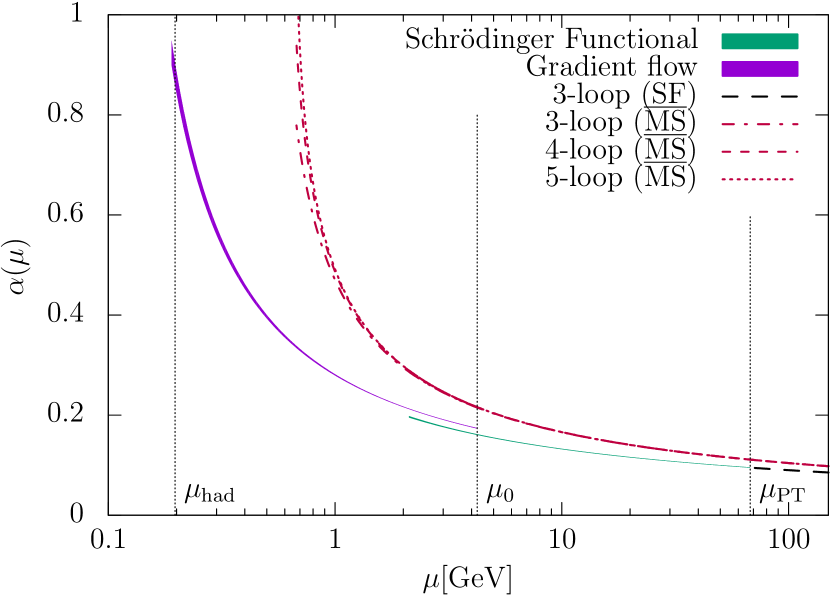
Figure 2: Running couplings of $N_{\mathrm{f}}=3$ QCD from integrating the nonperturbative $\beta$-functions in the SF and GF schemes Dalla Brida et al. (2016, 2017a). They are matched nonperturbatively by defining $\bar{g}_{\rm SF}^{2}(\mu_{0})=2.012$ and computing $\bar{g}_{\rm GF}^{2}(\mu_{0}/2)=2.6723(64)$.

In order to exploit the advantages of both finite-volume schemes, we use the GF scheme at low energies, between $\mu_{\rm had}$ and $\mu_{0}$. There we switch nonperturbatively to the SF scheme (see Figure 2). Then we run up to $\mu_{\rm PT}$. In this way, we connected hadronic scales to $\mu_{\rm PT}$ Dalla Brida et al. (2016, 2017a), cf. Table 1.

Table 2: Scale ratios and values of the coupling determined from nonperturbative running from $\mu_{\rm had}{}$ to $\mu_{0}/2$ in the GF and from $\mu_{0}$ to $\mu_{\rm PT}$ in the SF scheme.

$\bar{g}_{\rm GF}^{2}(\mu_{\rm had})$	$\bar{g}^{2}_{\rm SF}(\mu_{\rm PT})$	$\mu_{\rm PT}/\mu_{\rm had}{}$	$\Lambda_{\rm\overline{MS\kern-0.35002pt}\kern 0.35002pt}^{(3)}/\mu_{\rm had}{}$
11.31	1.193(5)	349.7(6.8)	1.729(57)
10.20	1.193(5)	322.2(6.3)	1.593(53)

In Table 2 we show our intermediate results for $\bar{g}_{\rm SF}^{2}(\mu_{\rm PT})$ and $\mu_{\rm PT}/\mu_{\rm had}$ for two choices of a typical hadronic scale $\mu_{\rm had}{}$ of a few hundred MeV. In addition, we give $\Lambda_{\rm\overline{MS\kern-0.35002pt}\kern 0.35002pt}^{(3)}/\mu_{\rm had}{}$, obtained by the NNLO perturbative asymptotic relation and the exact conversion to the ${\rm\overline{MS\kern-0.50003pt}\kern 0.50003pt}$ scheme. We have verified that the systematic uncertainty $\sim\alpha^{2}(\mu_{\rm PT})$ and power corrections $\sim(\Lambda/\mu_{\rm PT})^{k}$ from this limited use of perturbation theory at scales above $\mu_{\rm PT}$ are negligible compared to our statistical uncertainties Dalla Brida et al. (2016, 2017b).

IV Connection to the hadronic world

The second key element is the nonperturbative determination of $\mu_{\rm had}$ in units of the experimentally accessible $f_{\pi\mathrm{K}}$. Our determination is based on CLS ensembles Bruno et al. (2015b) of $N_{\mathrm{f}}=3$ QCD with $m_{{\rm u}}=m_{{\rm d}}\equiv\widehat{m}$ in large volume. It is convenient to define a scale $\mu_{\rm ref}$ by the condition

$$\bar{g}_{\infty}^{2}(\mu_{\rm ref})=1.6\pi^{2}\approx 15.8\,,$$ (11)

and trajectories in the (bare) quark mass plane $(\widehat{m},m_{{\rm s}})$ by keeping the dimensionless ratio

$$\phi_{4}=(m_{\rm K}^{2}+m_{\pi}^{2}/2)\,/\,\mu_{\rm ref}^{2}\,$$ (12)

constant. Moreover, we define a reference scale $\mu_{\rm ref}^{\star}$ at the symmetric point ($m_{{\rm u}}=m_{{\rm d}}=m_{{\rm s}}$) by

$$\mu_{\rm ref}^{\star}\equiv\mu_{\rm ref}\Big{|}_{\phi_{4}=1.11,\,m_{{\rm u}}=m_{{\rm d}}=m_{{\rm s}}}\,.$$ (13)

The requirement that the $\phi_{4}$=constant trajectory passes through the physical point, defined by

$$m_{\pi}^{2}/f_{\pi\mathrm{K}}^{2}=0.8341,\quad m_{\rm K}^{2}/f_{\pi\mathrm{K}}^{2}=11.21\,,$$ (14)

results in $\phi_{4}=1.11(2)$ in the continuum limit Bruno et al. (2017) and motivates the particular choice in eq. (13).

Since the combination $f_{\pi\mathrm{K}}$ has a weak and well understood dependence on the pion mass along trajectories with constant $\phi_{4}$, a precise extrapolation from the symmetric point to the physical point can be performed Bietenholz et al. (2010); Bruno et al. (2017), see Figure 3. Continuum extrapolations with four lattice spacings, $0.05\,{\rm fm}\lesssim a\lesssim 0.09\,{\rm fm}$, together with the PDG value of eq. (3), yield Bruno et al. (2017)

$$\mu_{\rm ref}^{\star}=478(7)\,{\rm MeV}\,.$$ (15)

Note that $\mu_{\rm ref}^{\star}$ is defined at a point with unphysical quark masses, where finite-size effects are smaller and simulations are easier than close to the physical point. This allows us to include in the following analysis a CLS ensemble at a fifth lattice spacing, $a\approx 0.039\,{\rm fm}$.

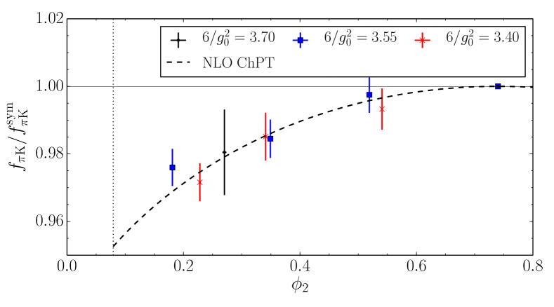
Figure 3: Dependence of $f_{\pi\mathrm{K}}$ at $\phi_{4}=1.11$ on the pion mass through $\phi_{2}=m_{\pi}^{2}/\mu_{\rm ref}^{2}$ Bruno et al. (2017). We normalized to $f_{\pi\mathrm{K}}^{\rm sym}$ at the symmetric point $m_{{\rm u}}=m_{{\rm d}}=m_{{\rm s}}$. The ratio follows the parameter-free prediction of NLO chiral PT.

For the determination of $\mu_{\rm ref}^{\star}/\mu_{\rm had}$, we need pairs of values $a\mu_{\rm had}{}$ and $a\mu_{\rm ref}^{\star}$ at the same value of $a$. This requires either an interpolation of the data for $a\mu_{\rm had}$, or an interpolation of the data for $a\mu_{\rm ref}^{\star}$. We denote these two options as set A and B, respectively.

The dimensionless ratio $\mu_{\rm ref}^{\star}/\mu_{\rm had}$ can then be extrapolated to the continuum as shown in Figure 4. Extrapolations, linear in $a^{2}$ dropping data above $(a\mu_{\rm ref}^{\star})^{2}=0.07$ with either set A or B, are fully compatible. They are also stable under changes in the number of points used to extrapolate and the particular functional form. These stabilities are expected since our smallest lattice spacing is $a\approx 0.039\,{\rm fm}$. We repeat the computation of $\mu_{\rm ref}/\mu_{\rm had}$ for two different values of $\mu_{\rm had}$ (see Figure 4). Tables of the various numbers that enter and further details can be found in the supplementary material.

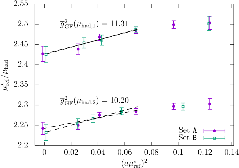
Figure 4: Continuum extrapolations described in the text. Extrapolated values are shown in proximity of $a=0$.

As our final estimates we take set B, which has somewhat larger errors, and obtain

$$\frac{\mu_{\rm ref}^{\star}}{\mu_{\rm had,1}}=2.428(18)\,,\quad\frac{\Lambda_{\rm\overline{MS\kern-0.35002pt}\kern 0.35002pt}^{(3)}}{\mu_{\rm ref}^{\star}}=0.712(24)\,,$$

(16)

$$\frac{\mu_{\rm ref}^{\star}}{\mu_{\rm had,2}}=2.233(17)\,,\quad\frac{\Lambda_{\rm\overline{MS\kern-0.35002pt}\kern 0.35002pt}^{(3)}}{\mu_{\rm ref}^{\star}}=0.713(24)\,.$$

The close agreement in $\Lambda_{\rm\overline{MS\kern-0.35002pt}\kern 0.35002pt}^{(3)}/\mu_{\rm ref}^{\star}$ is reassuring. With eq. (15) we arrive at our central result

$$\Lambda_{\rm\overline{MS\kern-0.35002pt}\kern 0.35002pt}^{(3)}=341(12)\,{\rm MeV}\,.$$ (17)

It has a remarkable precision given that we ran the couplings nonperturbatively up to about $70\,{\rm GeV}$ and only then used perturbation theory.

V $\Lambda$ parameters and coupling of five- and six-flavor theories

By itself our $\Lambda^{(3)}$ is of limited phenomenological use. The three-flavor effective field theory (EFT) is valid for energies below $m_{\mathrm{charm}}=1.28\,{\rm GeV}$. There perturbation theory cannot be expected to be precise.

However, QCD${}^{(N_{\mathrm{f}})}$, the $N_{\mathrm{f}}$-flavor effective theory, can be matched to QCD${}^{(N_{\mathrm{f}}+1)}$ and one can eventually arrive at QCD⁽⁶⁾ Weinberg (1973). This matching relates the couplings such that the low(er) energy EFT agrees with the (more) fundamental one up to power law corrections. These ${\rm O}(\Lambda^{2}/m_{\mathrm{h}}^{2})$ corrections can only be studied nonperturbatively. They are very small already for $m_{\mathrm{h}}=m_{{\rm charm}}$ Bruno et al. (2015a); Korzec et al. (2017).

Ignoring $1/m_{\mathrm{h}}^{2}$ effects, matching means

$$\bar{g}^{(N_{\mathrm{f}})}(\mu)=\bar{g}^{(N_{\mathrm{f}}+1)}(\mu)\,\times\,\xi\left(\bar{g}^{(N_{\mathrm{f}}+1)}(\mu),\frac{m_{\mathrm{h}}}{\mu}\right)$$

and the $\Lambda$ parameters are related by

$$\frac{\Lambda^{(N_{\mathrm{f}})}}{\Lambda^{(N_{\mathrm{f}}+1)}}=\frac{\varphi^{(N_{\mathrm{f}})}(\bar{g}^{(N_{\mathrm{f}}+1)}\times\xi)}{\varphi^{(N_{\mathrm{f}}+1)}(\bar{g}^{(N_{\mathrm{f}}+1)})}\,,$$ (19)

where

$$\varphi^{(N_{\mathrm{f}})}(\bar{g}) = (b_{0}\bar{g}^{2})^{-b_{1}/(2b_{0}^{2})}{\rm e}^{-1/(2b_{0}\bar{g}^{2})}$$

$$\times\exp\left\{-\int\limits_{0}^{\bar{g}}{\rm d}x\ \left[\frac{1}{\beta(x)}+\frac{1}{b_{0}x^{3}}-\frac{b_{1}}{b_{0}^{2}x}\right]\right\}\,$$

is defined in terms of the $N_{\mathrm{f}}$-flavor $\beta$-function in the chosen scheme.

Table 3: Main results of this work. $\Lambda_{\rm\overline{MS\kern-0.35002pt}\kern 0.35002pt}^{(3)}$, eq. (17), is determined nonperturbatively and used, together with the perturbative estimates of $\Lambda_{\rm\overline{MS\kern-0.35002pt}\kern 0.35002pt}^{(N_{\mathrm{f}})}/\Lambda_{\rm\overline{MS\kern-0.35002pt}\kern 0.35002pt}^{(3)}$, to produce all other numbers. As additional input we use the masses $m_{{\rm charm}}^{*}=1.280(25)\,{\rm GeV}$, $m_{\rm bottom}^{*}=4.180(30)\,{\rm GeV}$, $m_{\mathrm{Z}}=91.1876\,{\rm GeV}$, Patrignani et al. (2016) and $m_{\rm top}^{*}=165.9(2.2)\,{\rm GeV}$, Fuster et al. (2017).

$N_{\mathrm{f}}$	$\Lambda^{(N_{\mathrm{f}})}_{\rm\overline{MS\kern-0.35002pt}\kern 0.35002pt}$ [MeV]	$\mu$	$\alpha_{\rm\overline{MS\kern-0.35002pt}\kern 0.35002pt}^{(N_{\mathrm{f}})}(\mu)$
4	298(12)(3)
5	215(10)(3)	$m_{\mathrm{Z}}$	0.11852(80)(25)
6	91.1(4.5)(1.3)	$1.508\,\mathrm{TeV}$	0.08523(41)(12)

When inserting the perturbative expansions of $\xi$ and $\beta$, we choose the mass $m_{\mathrm{h}}$ in eq. (V) as the ${\rm\overline{MS\kern-0.50003pt}\kern 0.50003pt}$ mass at its own scale, $m^{*}=\kern 1.0pt\overline{\kern-1.0ptm\kern-1.0pt}\kern 1.0pt_{\rm\overline{MS\kern-0.35002pt}\kern 0.35002pt}(m^{*})$, and set $\mu=m^{*}$. Then the one-loop term vanishes in the perturbative expansion

$$\xi(\bar{g},1)=1+c_{2}\,\bar{g}^{4}+c_{3}\,\bar{g}^{6}+c_{4}\,\bar{g}^{8}+{\rm O}(\bar{g}^{10})\,.$$ (21)

For numerical results, we use $c_{2},c_{3},c_{4}$ Weinberg (1980); Bernreuther and Wetzel (1982); Grozin et al. (2011); Chetyrkin et al. (2006); Schröder and Steinhauser (2006) together with the appropriate five-loop $\beta$-function van Ritbergen et al. (1997); Czakon (2005); Baikov et al. (2017); Luthe et al. (2016); Herzog et al. (2017) to arrive at Table 3.

The first error in $\alpha(\mu)$ is due to $\Lambda_{\rm\overline{MS\kern-0.35002pt}\kern 0.35002pt}^{(3)}$ and the quark mass uncertainties, where the latter are hardly noticeable. The second error listed represents our estimate of the truncation error in PT in the connection $\Lambda_{\rm\overline{MS\kern-0.35002pt}\kern 0.35002pt}^{(3)}\to\Lambda_{\rm\overline{MS\kern-0.35002pt}\kern 0.35002pt}^{(4)}\,-\,\Lambda_{\rm\overline{MS\kern-0.35002pt}\kern 0.35002pt}^{(6)}$. We arrive at it as follows. The $2,3,4$-loop terms in eq. (21) combined with the $3,4,5$-loop $\beta$-functions in (V) lead, e.g., to contributions $128,\,19,\,6$ in units of $10^{-5}$ to $\alpha_{\rm\overline{MS\kern-0.35002pt}\kern 0.35002pt}(m_{\rm Z})$. We take the sum of the last two contributions as our perturbative uncertainty. Within PT, this is conservative. Recently, Herren and Steinhauser Herren and Steinhauser (2017) considered also $\mu\neq m$ in eq. (V). Their error estimate, $0.0004$, would change little in the uncertainty of our final result

$$\alpha_{\rm\overline{MS\kern-0.35002pt}\kern 0.35002pt}^{(5)}(m_{\mathrm{Z}})=0.11852(84)\,.$$ (22)

VI Summary and Conclusions

QCD offers a plethora of quantities, like hadron masses and meson decay constants, that can be used as precise experimental input to compute the strong coupling and quark masses. However, the nonperturbative character of the strong interactions makes these computations difficult. Lattice QCD offers a unique tool to connect, from first principles, well-measured QCD quantities at low energies to the fundamental parameters of the Standard Model. As perturbative expansions are not convergent, but only asymptotic, the challenge for precise results is to nonperturbatively reach energy scales where the strong coupling is small enough Dalla Brida et al. (2016). Due to the slow running of $\alpha_{s}$, the hadronic and perturbative regimes are separated by two to three orders of magnitude.

Finite-size scaling allows one to bridge such large energy differences nonperturbatively. It trades the systematic uncertainties associated with the truncation of the perturbative series at relatively low energies for statistical uncertainties which are easy to estimate.

Our precise data for the running coupling Dalla Brida et al. (2016, 2017a), together with the high-quality set of ensembles provided by the CLS initiative Bruno et al. (2015b) at lattice spacings as small as $a\approx 0.039\,{\rm fm}$, and an accurate determination of the scale Bruno et al. (2017), allow us to reach a precision of 0.7% in $\alpha_{\rm\overline{MS\kern-0.35002pt}\kern 0.35002pt}^{(5)}(m_{\mathrm{Z}})$.

The factor $\mu_{\rm PT}/\mu_{\rm had}$ contributes 87% of the uncertainty in $\alpha_{\rm\overline{MS\kern-0.35002pt}\kern 0.35002pt}^{(5)}$. This uncertainty is dominantly statistical and could certainly be reduced significantly by some additional effort. While present knowledge indicates small and perturbatively computable quark-loop effects in the matching at the heavy-quark thresholds, the uncomfortable need of using PT at scales as low as $m_{\mathrm{charm}}$ can only be avoided by a full four-flavor computation. This is a mandatory step as soon as one attempts another controlled reduction of the total uncertainty.

We finally note, that our result $\alpha_{\rm\overline{MS\kern-0.35002pt}\kern 0.35002pt}^{(6)}(1.508\,\mathrm{TeV})=0.0852(4)$ is in good agreement with the recent CMS determination Khachatryan et al. (2017) from jet cross sections with $p_{\mathrm{T}}\in[1.41,2.5]\,{\rm TeV}$. Ref. Khachatryan et al. (2017) gives $\alpha_{\rm\overline{MS\kern-0.35002pt}\kern 0.35002pt}^{(5)}(1.508\,{\rm TeV})=0.0822(33)$ which was already converted to $\alpha_{\rm\overline{MS\kern-0.35002pt}\kern 0.35002pt}^{(6)}(1.508\,{\rm TeV})=0.0840(35)$ in Herren and Steinhauser (2017). Although LHC data does not yet reach the precision of our result (evolved from lower energy), comparisons at such high energies are an excellent test of QCD and of the existence of massive colored quanta.

VII App: Supplementary material

Here we give some additional details concerning the new computation described in the section Connection to the hadronic world.

The continuum extrapolation of $\mu_{\rm ref}^{\star}/\mu_{\rm had}$ requires values of $a\mu_{\rm had}$ and $a\mu_{\rm ref}^{\star}$ at identical values of the improved bare coupling $\tilde{g}_{0}$ (as defined below). Thus, the determination of $\mu_{\rm ref}^{\star}/\mu_{\rm had}$ consists of three main parts

• $a\mu_{\rm had}$ vs. $g_{0}$ from simulations in finite volume

• $a\mu_{\rm ref}^{\star}$ vs. $\tilde{g}_{0}$ from simulations in large volume

• determination of $\mu_{\rm ref}^{\star}/\mu_{\rm had}$

which we now describe in detail.

VIII (I) $a\mu_{\rm had}$ vs. $g_{0}$ in finite volume

VIII.1 Lines of constant physics

A smooth continuum limit requires precise definitions of the renormalized parameters that are kept fixed while sending $a\to 0$. This defines the “lines of constant physics” for the choice of the bare parameters in the simulations. Since $\mu_{\rm had}$ is defined for massless quarks and in a finite volume with $\mu=1/L$, we choose the conditions

$$m(\mu_{\rm had,\it i})=0\,,$$ (23)

where $m(\mu)$ is the current quark mass defined through suitable Schrödinger Functional correlators Lüscher et al. (1996), and

$$\bar{g}^{2}_{\rm GF}(\mu_{\rm had,\it i})=u_{{\rm had,}i}\,,$$ (24)

with our values $u_{{\rm had,}1}=11.31$ and $u_{{\rm had,}2}=10.20$ for $\mu_{\rm had,1}$ and $\mu_{\rm had,2}$, respectively.

For a given $g_{0}$ and lattice size $L/a$, eq. (23) is equivalent to the determination of the critical values of the bare quark masses, $am_{\rm cr}(g_{0},a/L)$, at which the renormalized quark masses vanish. For later convenience it is useful to parametrize the deviation from the critical line by introducing the subtracted quark mass: $am_{\rm q}=am_{0}-am_{\rm cr}(g_{0},a/L)$, where $m_{{\rm u},0}=m_{\rm d,0}=m_{{\rm s},0}=m_{0}$ Lüscher et al. (1996) are the bare mass parameters of the lattice action.

The exact definition of $m$, i.e., the kinematical choices in the implementation of the PCAC relation, is given in Dalla Brida et al. (2017a). This leads to the results for $am_{\rm cr}(g_{0},a/L)$ reported in section A.1.4, specifically eq. (A.3) of this reference. This determination is available for $L/a=8,12,16$, and for the whole range of $g_{0}$ values we considered. In particular, these values of $m_{\rm cr}$ guarantee that $|Lm(1/L)|<0.005$, which is a stringent enough bound to let us assume that $m(1/L)$ is effectively zero in our analysis. We note, however, that below we shall consider also lattices with $L/a=20,24,32$ (and larger). For these, $am_{\rm cr}(g_{0},a/L)$ at a given $g_{0}$ was estimated by performing a linear extrapolation in $(a/L)^{3}$ of the critical hopping parameter, $\kappa_{\rm cr}(g_{0},a/L)=(2am_{\rm cr}(g_{0},a/L)+8)^{-1}$, using the results at the two largest available lattices, namely $L/a=12,16$. Examples of these kind of extrapolations are explicitly discussed in Fritzsch and Korzec .

VIII.2 Simulations and results for $a\mu_{\rm had}$

Table 4: List of all finite-volume ensembles that enter the hadronic matching computation. Here $\kappa=(2am_{0}+8)^{-1}$. The column labeled by $\bar{g}^{2}_{\rm GF}$ contains the values of the GF coupling as measured on the given ensembles. The values for the mass derivative ${\rm d}\bar{g}^{2}_{\rm GF}/{\rm d}am_{\rm q}$ instead are only given for ensembles with $am_{\rm q}=\Delta am_{\rm cr}\neq 0$. The coupling resulting from the shift to $am_{\rm q}=0$ is listed in the last column.

$L/a$	$6/g_{0}^{2}$	$\kappa$	$\bar{g}^{2}_{\rm GF}$	${\rm d}\bar{g}^{2}_{\rm GF}/{\rm d}am_{\rm q}$	$am_{\rm q}$	$\bar{g}^{2}_{{\rm GF},am_{\rm q}=0}$
$12$	$3.400000$	$0.136872258739141$	$11.308(97)$	$-$	$0$	$11.308(97)$
$12$	$3.480000$	$0.137038980000000$	$9.417(41)$	$-$	$0$	$9.417(41)$
$12$	$3.497000$	$0.137062990000000$	$9.118(54)$	$-$	$0$	$9.118(54)$
$12$	$3.500000$	$0.137066849094359$	$9.104(28)$	$-$	$0$	$9.104(28)$
$12$	$3.510000$	$0.137078900000000$	$8.897(46)$	$-$	$0$	$8.897(46)$
$12$	$3.532000$	$0.137101170000000$	$8.738(40)$	$-$	$0$	$8.738(40)$
$12$	$3.547000$	$0.137113150000000$	$8.460(38)$	$-$	$0$	$8.460(38)$
$16$	$3.530000$	$0.137142109937020$	$11.917(89)$	$-$	$0$	$11.917(89)$
$16$	$3.540000$	$0.137148520500305$	$11.565(82)$	$-$	$0$	$11.565(82)$
$16$	$3.556470$	$0.137032452074134$	$11.54(12)$	$87(10)$	$3.31\times 10^{-3}$	$11.25(11)$
$16$	$3.556470$	$0.137032452074134$	$11.39(11)$	$87(12)$	$3.31\times 10^{-3}$	$11.105(99)$
$16$	$3.560696$	$0.137036459478077$	$11.267(76)$	$83.2(76)$	$3.25\times 10^{-3}$	$10.996(71)$
$16$	$3.560696$	$0.137158587623782$	$10.982(64)$	$-$	$0$	$10.982(64)$
$16$	$3.629800$	$0.137163450000000$	$9.638(34)$	$-$	$0$	$9.638(34)$
$16$	$3.653850$	$0.137072212042003$	$9.250(69)$	$34.9(62)$	$2.22\times 10^{-3}$	$9.173(66)$
$16$	$3.657600$	$0.137154130000000$	$9.169(49)$	$-$	$0$	$9.169(49)$
$20$	$3.682900$	$0.137147800000000$	$11.404(73)$	$-$	$0$	$11.404(73)$
$20$	$3.790000$	$0.137048000000000$	$9.251(54)$	$-$	$0$	$9.251(54)$
$24$	$3.735394$	$0.137082625274551$	$12.87(16)$	$126(18)$	$6.51\times 10^{-4}$	$12.79(16)$
$24$	$3.793389$	$0.137020768592807$	$11.79(12)$	$101(13)$	$5.16\times 10^{-4}$	$11.74(12)$
$24$	$3.833254$	$0.136967740552669$	$10.497(78)$	$32.7(62)$	$4.47\times 10^{-4}$	$10.482(78)$
$24$	$3.936816$	$0.136798051283124$	$8.686(52)$	$19.2(40)$	$3.30\times 10^{-4}$	$8.680(52)$
$32$	$3.900000$	$0.136872019362733$	$13.36(15)$	$111(28)$	$1.53\times 10^{-4}$	$13.34(15)$
$32$	$3.976400$	$0.136730873919691$	$11.34(11)$	$61(22)$	$1.27\times 10^{-4}$	$11.34(11)$
$32$	$4.000000$	$0.136683960224116$	$10.91(13)$	$56(18)$	$1.22\times 10^{-4}$	$10.91(12)$
$32$	$4.100000$	$0.136473008507319$	$9.077(80)$	$29(14)$	$7.39\times 10^{-5}$	$9.075(78)$

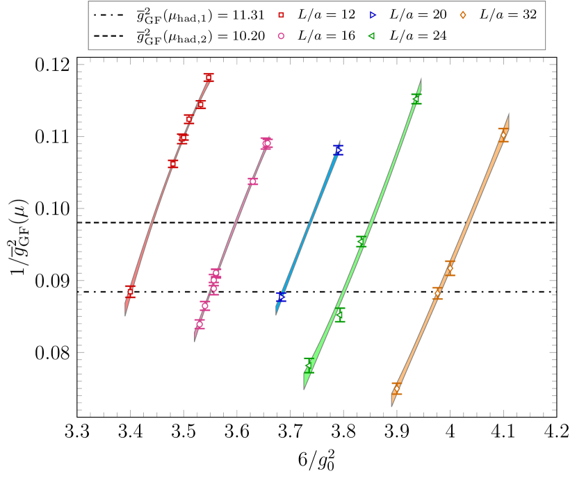
Figure 5: Interpolations $\bar{g}_{{\rm GF}}^{-2}=k_{0}+k_{1}(6/g_{0}^{2})+k_{2}(6/g_{0}^{2})^{2}$, performed separately for each $L/a$, with $k_{2}=0$ for $L/a=20$.

To perform the hadronic matching we collected many different ensembles with $L/a\in\{12,16,20,24,32\}$, at several values of $g_{0}$. These were used to determine pairs $(g_{0},L/a)$ for which the conditions (23) and (24) are satisfied. This is discussed in detail in the next section. The full set of ensembles is given in Table 4. For more than half of the ensembles the bare quark masses are such that $am_{\rm q}=0$, according to the definition of $am_{\rm cr}(g_{0},a/L)$ described above. For the others instead, we have $am_{\rm q}=\Delta am_{\rm cr}=am_{\rm cr}(g_{0},2a/L)-am_{\rm cr}(g_{0},a/L)$, because these ensembles originated as doubled lattices in the step scaling study of ref. Dalla Brida et al. (2017a). However, in order to have a smooth ${\rm O}(a^{2})$ dependence of the cutoff effects of our observables along lines of constant physics, all ensembles should have $m_{\rm q}=0$ according to a unique and specific definition (see e.g. ref. Lüscher et al. (1997)).

In order to achieve this, we computed in our MC-simulations the derivatives:

$$\frac{{\rm d}\bar{g}^{2}_{\rm GF}(\mu)}{{\rm d}am_{\rm q}}$$ (25)

on the ensembles with $am_{\rm q}\neq 0$, cf. Table 4. This information was then used to correct the measured values of $\bar{g}^{2}_{\rm GF}(\mu)$ on these ensembles in order to fulfill the condition $m_{\rm q}=0$. With the resulting values, $\bar{g}_{{\rm GF},am_{\rm q}=0}^{2}$, we can safely perform a smooth interpolation of the data for $\bar{g}_{{\rm GF},am_{\rm q}=0}^{2}$ to the target values $u_{{\rm had,}1}=11.31$ and $u_{{\rm had,}2}=10.20$.

At fixed $L/a$ we fit the data for $\bar{g}_{{\rm GF},am_{\rm q}=0}^{-2}$ as a function of $6/g_{0}^{2}$ using a second degree polynomial, except for the data at $L/a=20$ where a linear interpolation is used. These fits are all of excellent quality, except for $L/a=24$, see Figure 5. Our final interpolated pairs for $(g_{0},a\mu_{\rm had})$ are shown in Table 5, set B.

The improved bare coupling ${\tilde{g}_{0}}$ is defined as Lüscher et al. (1996); Bhattacharya et al. (2006)

$${\tilde{g}_{0}^{2}}=g_{0}^{2}\left(1+\tfrac{1}{3}{\rm tr}\{aM_{\rm q}\}\,b_{\rm g}(g_{0})\right)\,,$$ (26)

where $M_{\rm q}={\rm diag}(m_{\rm u,q},m_{\rm d,q},m_{\rm s,q})$ is the subtracted quark mass matrix and $b_{\rm g}(g_{0})$ is a given function of the bare coupling.

As discussed above, we have $m_{\rm u,q}=m_{\rm d,q}=m_{\rm s,q}=0$ in the ensembles used for the determination of $a\mu_{\rm had}$, and therefore ${\tilde{g}_{0}}=g_{0}$.

IX (II) $a\mu_{\rm ref}^{\star}$ vs. $\tilde{g}_{0}$ in large volume

IX.1 Improved coupling in CLS simulations

On the other hand, on the large volume CLS ensembles where $a\mu_{\rm ref}^{\star}$ has been computed, the value of ${\rm tr}\{aM_{\rm q}\}$ in (26) can be estimated using the results for $am_{i,0}$ given in ref. Bruno et al. (2017), and by taking for $am_{\rm cr}(g_{0},0)$ the corresponding result from the extrapolation of $\kappa_{\rm cr}(g_{0},a/L)$ described in the previous subsection.

Finally, at present, for the set-up of the CLS simulations, $b_{\rm g}(g_{0})$ is only known to one-loop order in perturbation theory. We thus used this value, which is given by Sint and Sommer (1996),

$$b_{\rm g}(g_{0})=0.036\,g_{0}^{2}+{\rm O}(g_{0}^{4})\,,\mbox{ for }N_{\rm f}=3\,.$$ (27)

Due to the smallness of ${\rm tr}\{aM_{\rm q}\}$, the difference between the bare couplings where the CLS simulations have been performed and the improved ones (see Table 5), is very small. The ${\rm O}(g_{0}^{4})$ uncertainty in eq. (27) is irrelevant at the level of our statistical uncertainties.

Our final values for $(\tilde{g}_{0},a\mu_{\rm ref}^{\star})$ after the correction $g_{0}\rightarrow\tilde{g}_{0}$ are shown in Table 5, set A. There, the first four results for $a\mu_{\rm ref}^{\star}$ are from Bruno et al. (2017), where also the exact definition of $\mu_{\rm ref}^{\star}$ at finite $a$ is specified. The fifth number is from a new simulation. Some details of this interesting simulation, close to the continuum, are given below.

IX.2 Simulation at the symmetric point and $6/g_{0}^{2}=3.85$

The CLS simulations, action and algorithm are described in Lüscher and Schaefer (2013); Bulava and Schaefer (2013); Bruno et al. (2015b, 2017) and the documentation of the openQCD code ope . To the ensembles already used in these publications, CLS has added a flavor-symmetric one at an even finer lattice spacing. It is a $192\times 64^{3}$ lattice with open boundary conditions, a lattice spacing of $a\approx 0.039$ fm and a hopping parameter of $\kappa=0.136852$. The general algorithmic setup follows the lines of the ones described in Bruno et al. (2015b), with only slight adjustments of the algorithmic mass parameters due to the finer lattice spacing. We have used a statistics of 6k molecular dynamics units (MDU) out of the available 6.5k.

The estimated integrated autocorrelation time of the GF topological charge at flow time $t=t_{0}$ is 0.3(2)k MDU and $\approx 0.1$k MDU for the action density $E(t_{0})$, cf. (10) of the main text. The latter is indistinguishable from $a\mu_{\rm ref}^{\star}$ concerning autocorrelations. We show the normalized autocorrelation function $\rho(t_{\mathrm{MC}})$ of $a\mu_{\rm ref}^{\star}$ in Figure 6. From $t_{\mathrm{MC}}\approx$ 0.2k MDU on, this function is compatible with zero within relatively large errors.

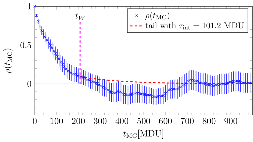
Figure 6: Normalized autocorrelation function, $\rho(t_{\mathrm{MC}})$ of $a\mu_{\rm ref}^{\star}$, as defined in Wolff (2004), and error estimate including a tail contribution (dashed curve), starting from $t_{\mathrm{W}}$.

For the determination of the integrated autocorrelation times, we use a slightly modified version of the procedure proposed in Schaefer et al. (2011). As usual, we sum $\rho(t_{\mathrm{MC}})$ within a window up to $t_{\mathrm{W}}$, for which we take the last $t_{\mathrm{MD}}$ at which $\rho(t_{\mathrm{MC}})$ is just one sigma away from zero. Above $t_{\mathrm{W}}$ we assume a single exponential decay with a decay rate given by the extrapolated value from previous simulations $\tau_{\mathrm{exp}}\approx 14\times t_{0}/a^{2}$, which corresponds to $\tau_{\mathrm{exp}}\approx 0.2$k MDU for this ensemble. Its amplitude is fixed by the central value of $\rho(t_{\mathrm{W}})$.

Note that the original procedure proposed in Schaefer et al. (2011) uses a smaller value of $t_{\mathrm{W}}$ which generally leads to larger autocorrelation times. In this sense, the procedure adopted here is less conservative than what is denoted “upper bound” in Schaefer et al. (2011), but more conservative than simply ignoring the tail. The hereby measured integrated autocorrelation times are compatible with the estimate of the extrapolated $\tau_{\mathrm{exp}}$, as expected for these slow quantities, which serves as a self-consistency check. With an estimated $\tau_{\mathrm{exp}}\approx 200$ MDU, our particular run has a total statistics of about 30 $\tau_{\mathrm{exp}}$, which is not what we would ideally like to have, but it is still (marginally) acceptable.

Table 5: Data of hadronic and reference scales and their ratio including continuum extrapolations. Set A refers to the $\tilde{g}_{0}^{2}$ values of the CLS simulations and set B to the integer values of $L/a=(a\mu_{\rm had})^{-1}$ of the small-volume simulations.

	$\mu_{\rm had,1}$				$\mu_{\rm had,2}$
set	$6/\tilde{g}_{0}^{2}$	$a\mu_{\rm ref}^{\star}$	$(a\mu_{\rm had})^{-1}$	$\mu_{\rm ref}^{\star}/\mu_{\rm had}$	$6/\tilde{g}_{0}^{2}$	$a\mu_{\rm ref}^{\star}$	$(a\mu_{\rm had})^{-1}$	$\mu_{\rm ref}^{\star}/\mu_{\rm had}$
A
	$3.3985$	$0.20899(20)$	$11.974(79)$	$2.503(17)$	$3.3985$	$0.20899(20)$	$11.017(68)$	$2.303(14)$
	$3.4587$	$0.18476(33)$	$13.524(46)$	$2.499(10)$	$3.4587$	$0.18476(33)$	$12.431(39)$	$2.297(08)$
	$3.549$	$0.15556(26)$	$15.971(34)$	$2.484(07)$	$3.549$	$0.15556(26)$	$14.688(49)$	$2.285(08)$
	$3.6992$	$0.12059(22)$	$20.460(60)$	$2.467(08)$	$3.6992$	$0.12059(22)$	$18.869(48)$	$2.275(07)$
	$3.8494$	$0.09437(19)$	$25.875(109)$	$2.442(11)$	$3.8494$	$0.09437(19)$	$23.846(93)$	$2.250(10)$
	Continuum extrapolations:				Continuum extrapolations:
	with $(a\mu_{\rm had})^{2}<0.07$			$2.426(18)$	with $(a\mu_{\rm had})^{2}<0.07$			$2.240(16)$
	with $(a\mu_{\rm had})^{2}<0.10$			$2.433(15)$	with $(a\mu_{\rm had})^{2}<0.10$			$2.247(11)$
B
	$3.3998$	$0.20845(19)$	$12.000(58)$	$2.501(12)$	$3.4407$	$0.19137(19)$	$12.000(34)$	$2.296(07)$
	$3.5498$	$0.15544(21)$	$16.000(30)$	$2.487(06)$	$3.5979$	$0.14282(19)$	$16.000(50)$	$2.285(08)$
	$3.6867$	$0.12304(21)$	$20.000(83)$	$2.461(11)$	$3.7372$	$0.11332(21)$	$20.000(64)$	$2.266(08)$
	$3.8000$	$0.10234(17)$	$24.000(105)$	$2.456(11)$	$3.8521$	$0.09396(19)$	$24.000(109)$	$2.255(11)$
	$3.9791$		$32.000(153)$		$4.0336$		$32.000(155)$
	Continuum extrapolations:				Continuum extrapolations:
	with $(a\mu_{\rm had})^{2}<0.07$			$\bf 2.428(18)$	with $(a\mu_{\rm had})^{2}<0.07$			$\bf 2.233(17)$

We finally mention that the simulation parameters yielded $\phi_{4}=1.108(7)$ and we thus had to perform only a very small shift in the quark masses to reach $\phi_{4}=1.11$, which is already accounted for in Table 5.

X (III) Determination of $\mu_{\rm ref}^{\star}/\mu_{\rm had}$

X.1 Interpolation of $a\mu_{\rm had}$ and $a\mu_{\rm ref}^{\star}$

The pairs $(\tilde{g}_{0},a\mu_{\rm had})$ and $(\tilde{g}_{0},a\mu_{\rm ref}^{\star})$ are not yet known at the same values of $\tilde{g}_{0}$. In order to obtain both $a\mu_{\rm ref}^{\star}$ and $a\mu_{\rm had}$ at equal values of the lattice spacing $a$, we have two possibilities: either we fit the values of $a\mu_{\rm had}$ as a function of $\tilde{g}_{0}$ and interpolate to the values of $\tilde{g}_{0}$ where $a\mu_{\rm ref}^{\star}$ is known, or we interpolate $a\mu_{\rm ref}^{\star}$ as a function of $\tilde{g}_{0}$ and determine its values at those $\tilde{g}_{0}$ where $a\mu_{\rm had}$ is known. These procedures have been labelled sets A and B, respectively in Table 5.

For the case of set A, $\log(a\mu_{\rm had})$ is fitted to a polynomial form

$$\log(a\mu_{\rm had})=\sum_{n=0}^{3}c_{n}(6/\tilde{g}_{0}^{2})^{n}\,,$$ (28)

which allows to determine values of $a\mu_{\rm had}$ at the $\tilde{g}_{0}^{2}$ where $a\mu_{\rm ref}^{\star}$ is known (set A of Table 5). We have repeated the whole analysis chain by replacing this interpolation by the purely heuristic (inverse) function $(6/\tilde{g}_{0}^{2})=\sum_{n=0}^{3}p_{n}(a\mu_{\rm had})^{-n}$, with entirely compatible results.

Regarding procedure B, the desired $a\mu_{\rm ref}^{\star}\equiv a/\sqrt{8t^{\scalebox{0.6}{\rm sym}}_{0}}$ as a function of $\tilde{g}_{0}$ is found in a very similar way. The functional form

$$\log(t_{0}^{\scalebox{0.6}{\rm sym}}/a^{2})=\sum_{n=0}^{3}a_{n}\,\left(\frac{6}{\tilde{g}_{0}^{2}}-3.5\right)^{n}\,,$$ (29)

describes our data very well ($\chi^{2}/{\rm dof}=0.5/1$) and is generally useful for scale setting. Its coefficients $a_{n}$ with covariances are listed in Table 6. Figure 7 shows the fit to the original CLS data and the interpolated values of $\log(a\mu_{\rm ref}^{\star})$

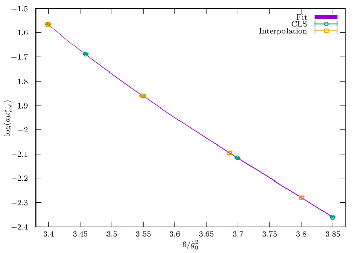
Figure 7: Fit of $\log(a\mu_{\rm ref}^{\star})$ to the points marked CLS. This fit allows us to read the values of $a\mu_{\rm ref}^{\star}$ at the values of $g_{0}$ where $a\mu_{\rm had,1}$ is known, set B (points labelled Interpolation).

at the values of $\tilde{g}_{0}$ determined from our data.

Table 6: Parameters $a_{n}$ and covariances ${\rm cov}(a_{n},a_{m})$ of our preferred parametrization, eq. (29).

$n$	$a_{n}\quad$	${\rm cov}(a_{n},a_{0})$	${\rm cov}(a_{n},a_{1})$	${\rm cov}(a_{n},a_{2})$	${\rm cov}(a_{n},a_{3})$
$0$	$1.45992$	$0.00001$	$0.00001$	$-0.00055$	$0.00129$
$1$	$3.78480$	$0.00001$	$0.00033$	$-0.00036$	$-0.00225$
$2$	$-2.10252$	$-0.00055$	$-0.00036$	$0.05423$	$-0.14131$
$3$	$2.71565$	$0.00129$	$-0.00225$	$-0.14131$	$0.40952$

X.2 Continuum extrapolation of $\mu_{\rm ref}^{\star}/\mu_{\rm had}$

The dimensionless ratio $\mu_{\rm ref}^{\star}/\mu_{\rm had}$ plotted in Figure 4 in the main text and listed in Table 5 can now be extrapolated to the continuum. We fit the data linearly in $a^{2}$, dropping either points above $(a\mu_{\rm ref}^{\star})^{2}=0.07$ or above $(a\mu_{\rm ref}^{\star})^{2}=0.1$. We performed this analysis with both sets A and B. The values at $a=0$ are fully compatible, see Table 5 and Figure 4 of the main text. We also extrapolated $\log(\mu_{\rm ref}^{\star}/\mu_{\rm had})$ and $(\mu_{\rm ref}^{\star}/\mu_{\rm had})^{-1}$, which of course have different higher order discretisation errors. Continuum values do not change by more than a per-mille. One may also combine sets A and B either after the extrapolation or before. That variant yields somewhat smaller errors and fully compatible central values in the continuum.

As our final estimate we take the numbers of set B extrapolated with data satisfying $(a\mu_{\rm ref}^{\star})^{2}\leq 0.07$ since these have the larger errors and in particular, since these make optimal use of our CLS point closest to the continuum at $a\approx 0.039\,{\rm fm}$. That data point is in any case crucial in stabilizing the continuum extrapolation. It renders the difference between the last data point and the extrapolated value insignificant and allows us to cite a continuum ratio with less than a percent error.

References

- Dittmaier et al. (2012) S. Dittmaier et al., (2012), 10.5170/CERN-2012-002, arXiv:1201.3084 [hep-ph] .
- Andersen et al. (2013) J. R. Andersen et al. (LHC Higgs Cross Section Working Group), (2013), 10.5170/CERN-2013-004, arXiv:1307.1347 [hep-ph] .
- Accardi et al. (2016) A. Accardi et al., Eur. Phys. J. C76, 471 (2016), arXiv:1603.08906 [hep-ph] .
- de Florian et al. (2016) D. de Florian et al. (LHC Higgs Cross Section Working Group), (2016), 10.23731/CYRM-2017-002, arXiv:1610.07922 [hep-ph] .
- Bardeen et al. (1978) W. A. Bardeen, A. J. Buras, D. W. Duke, and T. Muta, Phys. Rev. D18, 3998 (1978).
- Celmaster and Gonsalves (1979) W. Celmaster and R. Gonsalves, Phys. Rev. D 20, 1420 (1979).
- Patrignani et al. (2016) C. Patrignani et al. (Particle Data Group), Chin. Phys. C40, 100001 (2016).
- Aoki et al. (2009) S. Aoki et al. (PACS-CS), JHEP 0910, 053 (2009), arXiv:0906.3906 [hep-lat] .
- Lüscher et al. (1991) M. Lüscher, P. Weisz, and U. Wolff, Nucl. Phys. B359, 221 (1991).
- Lüscher et al. (1994) M. Lüscher, R. Sommer, P. Weisz, and U. Wolff, Nucl. Phys. B413, 481 (1994), arXiv:hep-lat/9309005 .
- de Divitiis et al. (1995) G. de Divitiis et al. (ALPHA), Nucl. Phys. B437, 447 (1995), hep-lat/9411017 .
- Jansen et al. (1996) K. Jansen, C. Liu, M. Lüscher, H. Simma, S. Sint, et al., Phys.Lett. B372, 275 (1996), hep-lat/9512009 .
- Dalla Brida et al. (2016) M. Dalla Brida, P. Fritzsch, T. Korzec, A. Ramos, S. Sint, and R. Sommer (ALPHA), Phys. Rev. Lett. 117, 182001 (2016), arXiv:1604.06193 [hep-ph] .
- Dalla Brida et al. (2017a) M. Dalla Brida, P. Fritzsch, T. Korzec, A. Ramos, S. Sint, and R. Sommer (ALPHA), Phys. Rev. D95, 014507 (2017a), arXiv:1607.06423 [hep-lat] .
- Bruno et al. (2015a) M. Bruno, J. Finkenrath, F. Knechtli, B. Leder, and R. Sommer (ALPHA), Phys. Rev. Lett. 114, 102001 (2015a), arXiv:1410.8374 [hep-lat] .
- Korzec et al. (2017) T. Korzec, F. Knechtli, S. Cali, B. Leder, and G. Moir, Proceedings, 34th International Symposium on Lattice Field Theory (Lattice 2016), PoS LATTICE2016, 126 (2017), arXiv:1612.07634 [hep-lat] .
- Aoki et al. (2016) S. Aoki et al., (2016), arXiv:1607.00299 [hep-lat] .
- Sommer and Wolff (2015) R. Sommer and U. Wolff, Proceedings, Advances in Computational Particle Physics: Final Meeting (SFB-TR-9), Nucl. Part. Phys. Proc. 261-262, 155 (2015), arXiv:1501.01861 [hep-lat] .
- Lüscher et al. (1992) M. Lüscher, R. Narayanan, P. Weisz, and U. Wolff, Nucl. Phys. B384, 168 (1992), arXiv:hep-lat/9207009 .
- Sint (1994) S. Sint, Nucl. Phys. B421, 135 (1994), hep-lat/9312079 .
- Fritzsch and Ramos (2013) P. Fritzsch and A. Ramos, JHEP 1310, 008 (2013), arXiv:1301.4388 [hep-lat] .
- González-Arroyo et al. (1983) A. González-Arroyo, J. Jurkiewicz, and C. Korthals-Altes, Structural Elements in Particle Physics and Statistical Mechanics, NATO ASI B82, 339 (1983), Proceedings, NATO Advanced Study Institute held in Freiburg, Germany, 31 Aug - 11 Sep 1981.
- Sint and Vilaseca (2012) S. Sint and P. Vilaseca, Proceedings, 30th International Symposium on Lattice Field Theory (Lattice 2012), PoS LATTICE2012, 031 (2012), arXiv:1211.0411 [hep-lat] .
- Bode et al. (1999) A. Bode, U. Wolff, and P. Weisz (ALPHA), Nucl. Phys. B540, 491 (1999), hep-lat/9809175 .
- Bode et al. (2000) A. Bode, P. Weisz, and U. Wolff (ALPHA), Nucl. Phys. B576, 517 (2000), [Erratum-ibid. B600 (2001) 453], [Erratum-ibid. B608 (2001) 481], hep-lat/9911018 .
- Lüscher (2010) M. Lüscher, JHEP 1008, 071 (2010), arXiv:1006.4518 [hep-lat] .
- Fodor et al. (2012) Z. Fodor, K. Holland, J. Kuti, D. Nogradi, and C. H. Wong, JHEP 11, 007 (2012), arXiv:1208.1051 [hep-lat] .
- Dalla Brida et al. (2017b) M. Dalla Brida, P. Fritzsch, T. Korzec, R. Ramos, S. Sint, and R. Sommer, in preparation (2017b).
- Bruno et al. (2015b) M. Bruno et al., JHEP 02, 043 (2015b), arXiv:1411.3982 [hep-lat] .
- Bruno et al. (2017) M. Bruno, T. Korzec, and S. Schaefer, Phys. Rev. D95, 074504 (2017), arXiv:1608.08900 [hep-lat] .
- Bietenholz et al. (2010) W. Bietenholz et al., Phys. Lett. B690, 436 (2010), arXiv:1003.1114 [hep-lat] .
- Weinberg (1973) S. Weinberg, Phys. Rev. D8, 3497 (1973).
- Fuster et al. (2017) J. Fuster, A. Irles, D. Melini, P. Uwer, and M. Vos, (2017), arXiv:1704.00540 [hep-ph] .
- Weinberg (1980) S. Weinberg, Phys. Lett. B91, 51 (1980).
- Bernreuther and Wetzel (1982) W. Bernreuther and W. Wetzel, Nucl. Phys. B197, 228 (1982), [Erratum: Nucl. Phys. B513, 758 (1998)].
- Grozin et al. (2011) A. G. Grozin, M. Hoeschele, J. Hoff, and M. Steinhauser, JHEP 09, 066 (2011), arXiv:1107.5970 [hep-ph] .
- Chetyrkin et al. (2006) K. G. Chetyrkin, J. H. Kühn, and C. Sturm, Nucl. Phys. B744, 121 (2006), arXiv:hep-ph/0512060 .
- Schröder and Steinhauser (2006) Y. Schröder and M. Steinhauser, JHEP 01, 051 (2006), arXiv:hep-ph/0512058 .
- van Ritbergen et al. (1997) T. van Ritbergen, J. A. M. Vermaseren, and S. A. Larin, Phys. Lett. B400, 379 (1997), arXiv:hep-ph/9701390 .
- Czakon (2005) M. Czakon, Nucl. Phys. B710, 485 (2005), arXiv:hep-ph/0411261 .
- Baikov et al. (2017) P. A. Baikov, K. G. Chetyrkin, and J. H. Kühn, Phys. Rev. Lett. 118, 082002 (2017), arXiv:1606.08659 [hep-ph] .
- Luthe et al. (2016) T. Luthe, A. Maier, P. Marquard, and Y. Schröder, JHEP 07, 127 (2016), arXiv:1606.08662 [hep-ph] .
- Herzog et al. (2017) F. Herzog, B. Ruijl, T. Ueda, J. A. M. Vermaseren, and A. Vogt, JHEP 02, 090 (2017), arXiv:1701.01404 [hep-ph] .
- Herren and Steinhauser (2017) F. Herren and M. Steinhauser, (2017), arXiv:1703.03751 [hep-ph] .
- Khachatryan et al. (2017) V. Khachatryan et al. (CMS), JHEP 03, 156 (2017), arXiv:1609.05331 [hep-ex] .
- Lüscher et al. (1996) M. Lüscher, S. Sint, R. Sommer, and P. Weisz, Nucl. Phys. B478, 365 (1996), arXiv:hep-lat/9605038 .
- (47) P. Fritzsch and T. Korzec, in preparation .
- Lüscher et al. (1997) M. Lüscher, S. Sint, R. Sommer, and H. Wittig, Nucl. Phys. B491, 344 (1997), arXiv:hep-lat/9611015 .
- Bhattacharya et al. (2006) T. Bhattacharya, R. Gupta, W. Lee, S. R. Sharpe, and J. M. Wu, Phys. Rev. D73, 034504 (2006), arXiv:hep-lat/0511014 .
- Sint and Sommer (1996) S. Sint and R. Sommer, Nucl. Phys. B465, 71 (1996), arXiv:hep-lat/9508012 .
- Lüscher and Schaefer (2013) M. Lüscher and S. Schaefer, Comput. Phys. Commun. 184, 519 (2013), arXiv:1206.2809 [hep-lat] .
- Bulava and Schaefer (2013) J. Bulava and S. Schaefer, Nucl. Phys. B874, 188 (2013), arXiv:1304.7093 [hep-lat] .
- (53) “openQCD – Simulation program for lattice QCD,” http://luscher.web.cern.ch/luscher/openQCD/.
- Wolff (2004) U. Wolff (ALPHA), Comput. Phys. Commun. 156, 143 (2004), [Erratum: Comput. Phys. Commun. 176, 383 (2007)], arXiv:hep-lat/0306017 .
- Schaefer et al. (2011) S. Schaefer, R. Sommer, and F. Virotta (ALPHA), Nucl. Phys. B845, 93 (2011), arXiv:1009.5228 [hep-lat] .