The Interstellar Medium and Star Formation of Galactic Disks.
I. ISM and GMC properties with Diffuse FUV and Cosmic Ray Backgrounds

Abstract

We present a series of adaptive mesh refinement (AMR) hydrodynamic simulations of flat rotation curve galactic gas disks with a detailed treatment of the interstellar medium (ISM) physics of the atomic to molecular phase transition under the influence of diffuse far ultraviolet (FUV) radiation fields and cosmic ray backgrounds. We explore the effects of different FUV intensities, including a model with a radial gradient designed to mimic the Milky Way. The effects of cosmic rays, including radial gradients in their heating and ionization rates, are also explored. The final simulations in this series achieve $4\>$pc resolution across the $\sim 20\>$kpc global disk diameter, with heating and cooling followed down to temperatures of $\sim 10\>$K. The disks are evolved for $300\>$Myr, which is enough time for the ISM to achieve a quasi-statistical equilibrium. In particular, the mass fraction of molecular gas stabilizes by $\sim$200 Myr. Additional global ISM properties are analysed. Giant molecular clouds (GMCs) are also identified and the statistical properties of their populations examined. GMCs are tracked as the disks evolve. GMC collisions, which may be a means of triggering star cluster formation, are counted and the rates compared with analytic models. Relatively frequent GMC collision rates are seen in these simulations and their implications for understanding GMC properties, including the driving of internal turbulence, are discussed.

1 Introduction

Most stars form in galactic disk systems, from “normal” disk galaxies to circumnuclear starburst disks (see, e.g., [Kennicutt & Evans (2012)]; [König et al. (2016)]). These disks can share a number of common properties, such as having approximately flat rotation curves (i.e., they are shearing disks) and being marginally gravitationally unstable (i.e., with a Toomre (1964) parameter $Q\sim 1$). Observational evidence has accumulated to connect star formation rates (SFRs) to the global disk environments (e.g., Kennicutt (1998); Bigiel et al. (2008); Genzel et al. (2010); Tan (2010); Suwannajak et al. (2014)). It is thus important to understand the processes controlling interstellar medium (ISM) dynamics and star formation activity in such systems.

There have been many previous numerical simulation studies of galactic disks. The most comparable set of simulations to our current work are those of Tasker & Tan (2009, hereafter TT09), Tasker (2011) and Tasker et al. (2015). TT09 presented a simulation of a galactic disk with total gas mass surface density ranging from about $\Sigma_{g}\simeq 60\>M_{\odot}\>{\rm pc}^{-2}$ at galactocentric radius $r=2\>$kpc to $\simeq 10\>M_{\odot}\>{\rm pc}^{-2}$ at $10\>$kpc, with maximum resolution of 8 pc that could undergo cooling to 300 K with a multi-phase ISM. The cooling floor of 300 K (i.e., a minimum sound speed of $c_{s}=1.6\>{\rm km\>s}^{-1}$) was an approximate method of modeling sub-grid turbulent support. For this reason, the detailed physics of the atomic to molecular transition was not followed in these simulations. The TT09 disk fragmented into a population of self-gravitating giant molecular clouds (GMCs), defined simply as connected, locally-peaked structures above a threshold density of $n_{\rm H}=100\>{\rm cm}^{-3}$, which were tracked and had their collision rates measured. However, this simulation did not include far ultraviolet (FUV) heating or any other feedback processes. It thus had a GMC mass fraction that was moderately too high, $\sim 2/3$, compared to, e.g., the Milky Way disk inside the solar orbit, which has a molecular mass fraction $f_{\rm mol}\equiv\Sigma_{\rm H2}/(\Sigma_{\rm H2}+\Sigma_{\rm HI})\simeq 0.75$ at $r=2\>$kpc falling to $\simeq 0.6$ at $5\>$kpc and $\simeq 0.2$ by $8\>$kpc (Koda et al., 2016). Also, GMCs in the TT09 simulation had typical mass surface densities, $\Sigma_{\rm GMC}\sim 300\>M_{\odot}\>{\rm pc}^{-2}$, i.e., about a factor of 2 to 3 times higher than observed Milky Way GMCs.

Tasker (2011) presented a simulation of the same disk set-up, but now including a constant diffuse FUV background with intensity of $G_{0}=4$, normalized according to Habing (1968), (i.e., 4 Habings, which is about 2.4 times the local value in the solar vicinity of $G_{0}=1.7$, Draine (1978)), which leads to photoelectric heating via dust grains. A model of star formation, i.e., star particle creation, above a fixed density threshold of $n_{\rm H,*}=100\>{\rm cm}^{-3}$ at constant efficiency per local free-fall time (Krumholz & Tan, 2007), but no feedback from young stars. One of the caveats of this simulation is that identified GMC properties were affected by the presence of clusters of star particles that could dominate the mass of the identified gaseous “GMC” structure. GMC dynamical properties and collision rates were thus affected by the presence of these star clusters. Tasker et al. (2015) included localized SNe feedback, in addition to the diffuse photoelectric heating. Their result suggests that weak localized thermal feedback may play a relatively minor role in shaping the galactic structure compared to gravitational interactions and disk shear. In both studies, very approximate heating/cooling physics only down to 300 K was adopted, and the atomic to molecular transition was not modeled. Fujimoto et al. (2014, 2016), utilizing the same simulation code and cooling function as TT09, investigated the GMC evolution in a M83-type barred spiral galaxy with 1.5 pc resolution. Frequent cloud-cloud and tidal interactions in the bar region help to build up massive GMCs and unbound, transient clouds.

With a “two-fluid” (isothermal warm and cold gas) model without thermal processes, Dobbs (2008) carried out isolated, magnetized disk simulations with an SPMHD code and studied GMC formation and evolution via agglomeration and self gravity in spiral galaxies with different surface densities. Dobbs et al. (2011) adopted diffuse FUV heating, radiative and collisional cooling, and a simple prescription of stellar energy feedback. It was found that the spiral arms do not significantly trigger star formation but help gather gas and increase collision rates to produce more massive and denser GMCs. The GMC mass function was approxiamately reproduced and similar populations of retrograde and prograde clouds (relative to the galaxy rotation) found due to enhanced collisions in the spiral arm regions (although TT09 saw a similar result without need for large-scale spiral arms). Dobbs et al. (2017) extended these models to study populations of star clusters formed in the disks and compared them with observed systems.

Other galactic disk simulations have been conducted to investigate the physical processes that influence disk evolution. The role of stellar feedback has been emphasized by, e.g., Agertz et al. (2013); Agertz & Kravtsov (2015); Hopkins et al. (2011, 2012, 2014). Hopkins et al. (2011, 2012) developed a set of numerical models to follow stellar feedback on scales from sub-GMC star-forming regions through entire galaxies, including the energy, momentum, mass, and metal fluxes from stellar radiation pressure, HII photoionization and photoelectric heating, Types I and II SNe, and stellar winds (O-star and AGB). Based on the models, Hopkins et al. (2012, 2013) conducted pc-resolution SPH simulations of three types of isolated galaxies, i.e., SMC, Milky Way and Sbc, and produce a quasi-steady ISM in which GMCs form and disperse rapidly, with phase structure, turbulence, and disk and GMC properties concluded to be in good agreement with observations. Mayer et al. (2016) studied disk fragmentation and formation of giant clumps regulated by turbulence via superbubble or blastwave supernovae feedback, using the GASOLINE2 SPH code and the lagrangian mesh-less code GIZMO. The difference in clump properties between the two sources of turbulence are found as a potential test of feedback mechanisms.

Goldbaum et al. (2015, 2016) investigated the driving of turbulence by gravitational instabilities and star formation feedback, including stochastic stellar population synthesis, HII region feedback, SNe and stellar winds via 20-pc-resolution AMR hydrodynamics simulations. They argue from their results that gravitational instability is likely to be the dominant source of turbulence and transport in galactic disks, and that it is responsible for fueling star formation in the inner parts of galactic disks over cosmological times. The cascade of turbulence to smaller scales may be one process that regulates the local star formation rate within GMCs (Padoan & Nordlund, 2002; Krumholz & McKee, 2005), which is known to occur at a low efficiency per local free-fall time (Zuckerman & Evans, 1974; Krumholz & Tan, 2007).

In this work, our overall goal is to understand how the interstellar medium, including GMCs, and star formation activity in galactic disk systems is regulated, ultimately modeling all important physical processes and determining their relative importance, including in different galactic environments. In this first paper we introduce our fiducial “normal” disk model and our methods of treating the microphysics of ISM heating and cooling processes. We start with the simplifying assumption of only considering FUV and CR heating, which can both be approximated as diffuse components. The first main goal is to understand ISM structure, including GMC structural and dynamical properties, in this limiting case, before complexities of magnetic fields, star formation and localized feedback are introduced (deferred to future papers in this series). Compared to the simulations of TT09 the main improvements are: 1) we follow heating and cooling down to $\sim 10\>$K; 2) we use much improved heating and cooling functions that we develop in this paper based on photodissociation region (PDR) calculations (for up to four dimensional grids of density, temperature, FUV intensity and cosmic ray ionization rate, adopting an empirical extinction versus density relation to allow local evaluation); 3) a variable mean particle mass across the atomic to molecular transition is allowed for in the hydrodynamic equations; 4) we study models, step by step, that investigate the effects of a variety of different assumptions of the FUV radiation field, including a model with a radial gradient within the disk; 5) we reach higher resolutions of 4 pc.

In §2 we explain our simulation setup and methods. We present our results on global ISM properties in §3. We examine GMC properties in §4 and discuss GMC collisions in §5. We conclude in §6.

2 Methods

2.1 Numerical Code and Simulation Suite

The simulations presented in this paper were run using the numerical code Enzo, an adaptive mesh refinement (AMR) hydrodynamics code (Bryan et al., 2014). This code solves the hydrodynamics equations using the 3D Zeus hydrodynamics solver (Stone & Norman, 1992), which uses an artificial viscosity term to handle shocks. The quadratic artificial viscosity parameter (von Neumann & Richtmyer, 1950) was set to 2.0 (the default value) for all simulations.

For most simulations (Runs I to V), we use a root grid (32.768 kpc on each side) of $256^{3}$ and 4 additional AMR levels, giving a minimum spatial resolution of 8 pc. Cells are refined when the local Jeans length becomes smaller than 4 cell-widths, which is the condition typically used to avoid artificial fragmentation (Truelove et al., 1997). For comparison with the results of TT09, in Runs I, II and III, we first study disks that have a temperature floor of 300 K, which corresponds to the upper range of temperatures of the atomic cold neutral medium (CNM) (Wolfire et al., 2003). We then adopt a 10 K temperature floor (Run IV, V and VI) to more accurately follow the atomic to molecular transition and thus the properties of GMCs. In Run VI we also introduce an extra level of AMR refinement, i.e., 5 levels in total, achieving 4 pc resolution to better resolve cloud structures. Note, however, that with temperatures now followed to 10 K, the Jeans length may not be well resolved above densities of $\sim$ 400 cm^-3. Artificial fragmentation may be occurring above these densities, which should be kept in mind when interpreting some of the results.

In this paper, we aim to examine the formation and evolution of GMCs in a flat rotation curve galactic disk without consideration of star formation, magnetic fields and localized feedback mechanisms. We mainly study the effects of diffuse FUV feedback and the influence of diffuse cosmic ray (CR) ionization/heating. To investigate the influence of diffuse FUV feedback, we present simulation runs with different static FUV background radiation fields. In Runs I and II we set up a constant diffuse FUV radiation field with $G_{0}$ = 1.0, 4.0, respectively, where $G_{0}=1$ is the FUV intensity normalized to the Habing (1968) estimate and a value of $G_{0}=1.7$ corresponds to the local FUV radiation field in the Milky Way disk (Draine, 1978). In Run III, the FUV field is set following the profile from Wolfire et al. (2003), where we take a local value of $G_{0}(R_{0})=1.7$ (Draine, 1978). In Run I to III, the CR ionization rate is set to a constant value $\zeta=1\times 10^{-16}\>$s^-1 (e.g., Dalgarno (2006)). $G_{0}$ and $\zeta$ are both input parameters of the PDR models. The configuration of each run is summarized in Table 2.1.

Configurations of simulations. Run Resolution (pc) $T_{\mathrm{floor}}$ (K) $G_{0}$ $\zeta$ (${\rm s^{-1}}$) I 8 300 4 $10^{-16}$ II 8 300 1 $10^{-16}$ III 8 300 Wolfire^a $10^{-16}$ IV 8 10 Wolfire $10^{-16}$ V 8 10 Wolfire $\zeta(r)$ ^b VI 4 10 Wolfire $10^{-16}$ ^a FUV intensity radial profile from Wolfire et al. (2003).
^b Linearly gradient from $\zeta=5\times 10^{-16}$ s^-1 at $r=2\>$kpc to $5\times 10^{-17}$ s^-1 at $r=10\>$kpc.

To better track the atomic to molecular transition, we then carry out several runs with a 10 K temperature floor. This also permits investigation of the effects of CR ionization, which mostly influences the chemistry and heating of cooler, denser (i.e., highly-extinguished) molecular gas (i.e., $T<30\>$K, $A_{V}>10$ mag, i.e., $n_{\rm H}>10^{3}$ $\mathrm{cm^{-3}}$; see Bisbas et al. (2015)). Note that the temperature floor is not necessarily reached in the simulations. In Run IV we use a CR ray ionization rate $\zeta=1\times 10^{-16}\mathrm{\ s}^{-1}$, while Run V adopts a simple linear radial profile with the maximum and minimum equal to $5\times 10^{-16}$ (at $r=2\>$kpc) and $5\times 10^{-17}\>$s^-1 (at $r=10\>$kpc), respectively. Run VI uses the same constant value of $\zeta$ as in Run IV, but now introduces an extra level of AMR to yield 4 pc resolution.

2.2 Initial Conditions

Following TT09, we initialize an isolated self-gravitating gas disk, rotating around the $z$-axis, in a static gravitational background potential. This potential is described by (Binney & Tremaine, 1987)

$$\phi_{\rm bg}=\frac{1}{2}v_{c,0}^{2}\ln\left[\frac{1}{r_{c}^{2}}\left(r_{c}^{2}+r^{2}+\frac{z^{2}}{q_{\phi}^{2}}\right)\right],$$ (1)

i.e., identical to that adopted by TT09, which yields a flat rotation curve with $v_{c,0}=200\>\mathrm{km\>s^{-1}}$ at galactocentric radii $r\gg r_{c}=0.5\>\mathrm{kpc}$. The axial ratio of the potential field is $q_{\phi}=0.7$. The distribution of the background dark matter and stellar population would in reality evolve in response the changing distribution of ISM gas mass (e.g., Read et al. (2016)), however, this effect is not included here given our focus on determining ISM structure that occurs in a given galactic potential.

The initial density profile of the gas disk is set to be

$$\rho(r,z)=\frac{\kappa c_{s}}{2\pi GQz_{h}}\mathrm{sech^{2}}\left(\frac{z}{z_{h}}\right)\>\>(r<12\ \mathrm{kpc}),$$ (2)

where the scale height $z_{h}$ is set to 290 pc, and for purposes of normalization of the initial condition, the sound speed $c_{s}$ is set equal to $7.7\>\rm km\>s^{-1}$. These choices are made so that the initial Toomre (1964) stability parameter, i.e., with input quantities averaged in annuli in the disk, is $Q=1.5$ for $2\mathrm{\ kpc}<r<10\mathrm{\ kpc}$, which is our only region of interest, and $Q=20$ at the same sound speed for $r<2\mathrm{\ kpc}$ or $10\mathrm{\ kpc}<r<12\mathrm{\ kpc}$, which are boundary regions. The epicyclic frequency $\kappa$ is expressed by

$$\kappa=\sqrt{2}\frac{v_{\rm circ}}{r}(1+\beta)^{\frac{1}{2}},$$ (3)

where $v_{\rm circ}$ is the circular velocity, which is equal to $v_{c,0}r(r_{c}^{2}+r^{2})^{-1/2}$ set by the gravitational potential of equation (1), and $\beta=\mathrm{d}\ln v_{\rm circ}/\mathrm{d}\ln r$. In total, the disk gas mass is $\sim 6\times 10^{9}\>M_{\odot}$.

The disk is surrounded by a quasi-static, dynamically negligible ambient medium with initial gas density

$$\rho_{\rm ambient}=\rho_{0}{\rm exp}{\left(-\frac{\mu m_{\mathrm{H}}}{kT}\phi\right)},$$ (4)

where the gravitational potential $\phi$ includes the contribution of background potential and the galactic gas disk. In our simulation, the maximum value of the initial ambient density is $n_{\mathrm{H}}=10^{-4}\>\mathrm{cm^{-3}}$ (approximately $10^{-4}$ of that in the main disk). We set its initial temperature to be $10^{6}$ K. The ambient density starts to dominate over that of the main disk component at several disk scale heights, e.g., at a height of $\sim$1.4 kpc at $r\sim 4$ kpc.

As discussed below, the gas undergoes heating and cooling processes. The net effect of the evolution from the initial condition is cooling, which leads to a reduction of $Q$ and thus fragmentation in the main disk region. Note, we adopt $c_{s}=\sqrt{\gamma kT/\mu}$ with a fixed adiabatic index $\gamma=5/3$. In the limit of fully molecular $\rm H_{2}$, the mean molecular weight $\mu=2.33m_{\mathrm{H}}$ (i.e., we assume 0.1 He per H and ignore contributions from other species, including $1\times 10^{-4}$ C and $3\times 10^{-4}$ O per H). The true mean molecular weight $\mu$ varies based on thermal processes (determined in an iterative way, see §2.3). We adopt the value of $\gamma=5/3$ for the entire simulation domain. While this does not account for the excitation of rotational and vibrational modes of $\rm H_{2}$ that would occur in shocks, we consider that this is the most appropriate single-valued choice of $\gamma$ for our simulation setup, given our focus on the dynamics of the dense molecular gas and given the resolutions that are achieved in the models, including allowance for the fact that the Zeus solver itself does not allow for very accurate shock capturing.

2.3 Heating and Cooling Functions

To investigate the effects of diffuse FUV heating and CR ionization, we implement PDR-based heating and cooling functions. The method is based on that developed by Wu et al. (2015) in the context of simulations of GMC collisions and for the simple case of a fixed background FUV intensity ($G_{0}=4$) and CR ionization rate ($\zeta=10^{-16}\>{\rm s}^{-1}$). For $T<10^{4}\>$K, we use the PYPDR code, which includes $\sim 30$ species and performs well in producing results similar to larger PDR codes up to $\sim 10^{4}\>$K (Röllig et al., 2007). PYPDR is also more flexible in being able to be adapted to calculate self-consistent grids of models at non-equilibrium conditions, including molecular self-shielding effects (see Wu et al. (2015)). For $T>10^{4}\>$K, we utilize the CLOUDY code (Ferland et al., 2013) (PYPDR is not designed to operate at these temperatures).

In each cell there are four parameters that are important for setting the chemical conditions and thus the (non-equilibrium) heating and cooling rates: gas number density of H nuclei ($n_{\mathrm{H}}$), gas temperature ($T$), local FUV intensity ($G_{0}$) and CR ionization rate ($\zeta$). The local FUV intensity is derived given $G_{0}$ (which may vary with galactocentric radius) and the visual extinction, $A_{V}$, to a cell. The method of Wu et al. (2015) involves approximating $A_{V}$ as a local, monotonically rising function of density $n_{\mathrm{H}}$. The reliability of this approximation on the scales of GMCs has been investigated by comparison with full radiative transfer simulations of Bisbas et al. (in prep.) and found to be accurate to $\sim$20% for heating and cooling rates at typical densities of $n_{\rm H}=10^{3}\>{\rm cm^{-3}}$ and temperatures of $T=100\>$K. More generally, on galactic scales, the validity of local approximations to account for FUV radiative shielding in multi-dimensional simulations has been studied comparing to a more accurate ray-tracing-based approach (Safranek-Shrader et al., 2017) and is reported to be physically appropriate to model the thermal impact of the HI–${\rm H_{2}}$ and CII/CI/CO transitions.

In this paper we have extended the grid of heating and cooling functions to span extra dimensions of $G_{0}$ and $\zeta$, i.e., up to a four dimensional parameter space. The range of background diffuse FUV intensities and cosmic ray ionization rates are set as described in §2.1. The heating/cooling functions span the density and temperature space of $10^{-4}<n_{\mathrm{H}}/\mathrm{cm}^{−3}<10^{6}$ and $2.7<T/\mathrm{K}<10^{7}$, covering our regime of interest.

The resulting heating/cooling rates and corresponding mean molecular weights are incorporated into Enzo via the Grackle external chemistry and cooling library (Smith et al., 2017). The information is read in via the purely tabulated mode using quadrilinear interpolation to fill the entire 4-D parameter space, and modifies the specific gas internal energy $e=p/(\gamma-1)$ of a given cell with a net heating/cooling rate calculated by

$$H=n_{\mathrm{H}}[\Gamma-n_{\mathrm{H}}\Lambda]\mathrm{\ erg\ cm^{-3}\ s^{-1}},$$ (5)

where $\Gamma$ is the heating rate and $\Lambda$ is the cooling rate. The species abundances and their line emissivities are also used to make predictions of emission line diagnostics (discussed in the next subsection).

2.4 Observational Diagnostics

One important output of the PDR model described in §2.3 is the detailed information about specific components that contribute to the radiative cooling rates. Given the local volume emissivities, $j$, of particular lines such as [CII] emission at 158 $\rm\mu m$ and rotational lines of ${}^{12}\mathrm{CO}$ and ${}^{13}\mathrm{CO}$, we are able to create synthetic integrated intensity maps in post-processing.

We note that radiative transfer is incorporated, approximately, in each cell through implementation in the 1D PDR models, while (for the results presented in this paper) full line radiative transfer is not calculated during post-processing, i.e., we sum contributions along lines of sight, which is only fully valid in the optically thin limit.

Thus we typically choose to study lines in which optical depths should be relatively small. The resulting intensities are simply integrated directly through the simulation domain. We also note that CO freeze-out onto dust grains is not yet treated in our PDR models. Following equation (6) in Wu et al. (2015), the integrated intensity is calculated through

$$\int T_{\mathrm{mb}}\mathrm{d}v=\frac{\lambda^{3}}{2k_{B}}I=\frac{\lambda^{3}}{2\pi k_{B}}\int_{\mathrm{LOS}}j\mathrm{d}z,$$ (6)

where $T_{\mathrm{mb}}$ is the main-beam temperature, $j$ is the emissivity (the output of PDR codes is $4\pi j$), $v$ is the line-of-sight velocity, $\mathrm{d}z$ is the line element along the line of sight, and $\lambda$ is the chosen line centroid wavelength.

2.5 Cloud Tracking

The clouds in the galactic disk were located using a number density of H nuclei threshold of $n_{\rm\mathrm{H},GMC}=100\ \mathrm{cm^{-3}}$, i.e., the same value used in the TT09 study and similar to the volume-averaged mean densities of typical Galactic GMCs. We will also justify this choice of density threshold based on the PDR models implemented in our simulations. When we refer to “clouds” or “GMCs” we are describing the gas that has achieved densities of at least $n_{\rm\mathrm{H},GMC}$.

Clouds are identified utilizing k-d tree, a binary-space-partitioning data structure especially effective in the proximity/clustering search, through the following loops, which achieve the same results as the method developed by TT09:

• Loop 1: local density peaks are identified within the cells with $n_{\mathrm{H}}>n_{\rm\mathrm{H},GMC}$. If the distance between two peaks is smaller than the deblending length (here we set it to a fixed distance of 32 pc, including in the run with 4 pc resolution), then only the peak with the higher density is retained as a “peak.”

• Loop 2: for every peak, adjacent cells with $n_{\mathrm{H}}>n_{\rm\mathrm{H},GMC}$ are marked as “belonging to the peak,” and cells adjacent to these marked cells are recursively marked in the same way. Eventually, the cells that have continuous spatial connections with multiple peaks are assigned to the peak closest to them, i.e., each cell is only assigned to one peak. With this method, multiple clouds can exist in the same continuous density structure, if it contains more than one well-separated peak.

Once clouds are identified for each simulation output, we then calculate their physical properties and also track cloud evolution. The clouds at $t_{0}$ and those at $t_{1}$ (typically $t_{1}-t_{0}=1$ Myr) are linked as parent–child pairs through the following steps:

• Step 1: assuming constant velocity within 1 Myr, a predicted center of mass at $t_{1}$ for each cloud found at $t_{0}$ is calculated.

• Step 2: a volume of radius 50 pc, larger than the expected deviations due to typical accelerations, centered on the predicted position of each cloud is searched for clouds present at time $t_{1}$. If multiple clouds are found in this region at $t_{1}$, the nearest one is linked with the cloud at $t_{0}$.

• Step 3: in the case that multiple $t_{0}$ clouds (parents) are linked to the same $t_{1}$ cloud (child) based on the previous step, the child will be assigned to the “parents” with the nearest predicted $t_{1}$ location. Other “parents” will repeat step 2 and search for alternative children excluding the assigned one until no conflict exists, or no alternative child exists so that the children defined in step 2 have to be linked to those “parents.”

• Step 4: if no clouds at $t_{1}$ are linked with the $t_{0}$ cloud, then a volume with radius equal to $3\times$ the average radius (defined as $R_{c}=\sqrt{A_{c}/\pi}$ where $A_{c}$ is projected area of the cloud in the $x$-$y$ plane) of the $t_{0}$ cloud is searched. This allows for large, extended clouds whose centers may have shifted due to external perturbations.

• Step 5: if multiple clouds at $t_{0}$ are linked to one cloud at $t_{1}$, then the most massive $t_{0}$ cloud is claimed to survive while others are “destroyed” by merger. If one $t_{0}$ cloud has no child, then it is claimed to have been destroyed by non-merger processes. Cloud formation is claimed for each $t_{1}$ cloud without any parent.

This procedure tracks merger events accurately, but we caution that this simple prescription for identifying destruction events may have difficulties, particularly when strong feedback mechanisms are eventually included. Still, the prescription works well in the current simulation, since we have limited cloud destruction, i.e., the diffuse FUV radiation does not lead to significant GMC destruction.

3 Large-Scale ISM Properties

In the following sections, we restrict our analysis of ISM and GMC properties to galactocentric radii between 2.5 and 8.5 kpc in order to avoid structures affected by the boundaries of the main disk.

3.1 Global Disk

The time evolution of the galactic disks of Runs I to VI are shown in Figures 1, 2, 3, 4, 5 and 6, respectively. At the beginning, with an initialized velocity dispersion of $\sigma_{g}=c_{s}\simeq 8\ \mathrm{km\ s^{-1}}$, the disks are marginally stable. As a result of radiative cooling, the disks become unstable and fragment into overdense structures, which increases the self-shielding from the diffuse FUV radiation, raises line cooling rates, thus leading to more rapid cooling and gathering of material from the surroundings. As overdense regions become denser than $n_{\rm\mathrm{H},GMC}=100\>\mathrm{cm^{-3}}$, they are identified as components of GMCs. Similar to the results seen by TT09, this evolution, driven by cooling, occurs most rapidly in the denser inner regions and therefore the first structure to form is an overdense ring near the inner boundary due to the Toomre ring instability. The instability gathers material from a range of radii about equal to the Toomre length, $\lambda_{T}=2\pi^{2}G\Sigma_{g}/\kappa^{2}$. The instability then propagates to outer regions as radiative cooling continues. Overdense local spiral patterns form and fragment into clouds.

Since the early phase evolution is quite artificial, in Figures 1 to 6 we focus on later stages from 100 to 300 Myr, showing also intermediate stages at 200 and 250 Myr. Later we will be focussing on the statistics of ISM and GMC properties from 200 to 300 Myr.

Comparing the first three runs (Figures 1 to 3), which have different FUV intensities, we see that energy injection from FUV radiation suppresses the growth of gravitational instabilities, especially in the lower density outer regions, thus shaping the spatial distribution as well as the global evolutionary history of GMCs. On the global scales viewed in Figures 1 to 6, there appear to be only modest effects on the dense gas structures caused by lowering the temperature floor from 300 K to 10 K, i.e., comparing Run III and Run IV. Applying a radially variable $\zeta$ in Run V, which overall has stronger heating than the constant $\zeta$ case, we see that fragmentation is delayed to some extent. CR heating is of greater importance in the denser, molecular phase where FUV radiation is shielded and equilibrium temperatures are lower.

Figure 1: Evolution of the galactic disk for Run I ($G_{0}=4$) (100, 200, 250 and 300 Myr from left to right). Images are 20 kpc across and show the disk gas mass surface density $\Sigma$ (top row) and mass-weighted temperature $T$ (bottom row), integrated vertically over the disk (over a range $-1\>{\rm kpc}<z<+1\>{\rm kpc}$).

Figure 2: Same as Fig. 1, but for Run II ($G_{0}=1$).

Figure 3: Same as Fig. 1, but for Run III (radially variable $G_{0}$).

Figure 4: Same as Fig. 1, but for Run IV (radially variable $G_{0}$ with 10 K temperature floor).

Figure 5: Same as Fig. 1, but for Run V (radially variable $G_{0}$ and $\zeta$ with 10 K temperature floor).

Figure 6: Same as Fig. 1, but for Run VI (radially variable $G_{0}$ with 10 K temperature floor and 4 pc resolution).

Figure 7: The evolution of azimuthally averaged radial profiles of gas mass surface density $\Sigma=\int_{-1\ \mathrm{kpc}}^{+1\ \mathrm{kpc}}\rho dz$ for Run I (upper left, $G_{0}$=4), II (upper middle, $G_{0}$=1), III (upper right, radially variable $G_{0}$), IV (lower left, radially variable $G_{0}$, 10 K temperature floor), V (lower middle, radially variable $G_{0}$ and $\zeta$, 10 K temperature floor), VI (lower right, radially variable $G_{0}$, constant $\zeta$, 10 K temperature floor with 4 pc resolution).

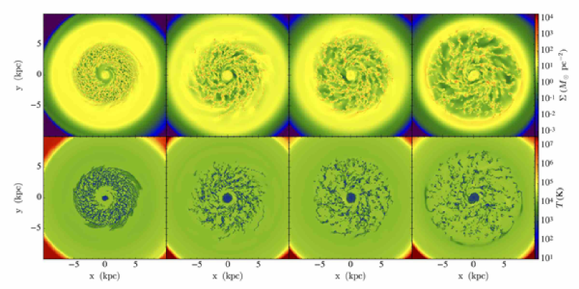
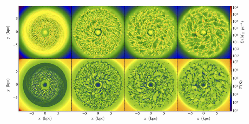
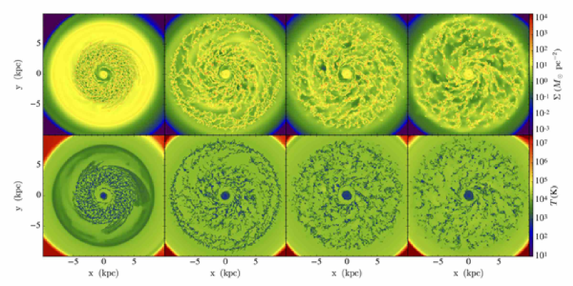
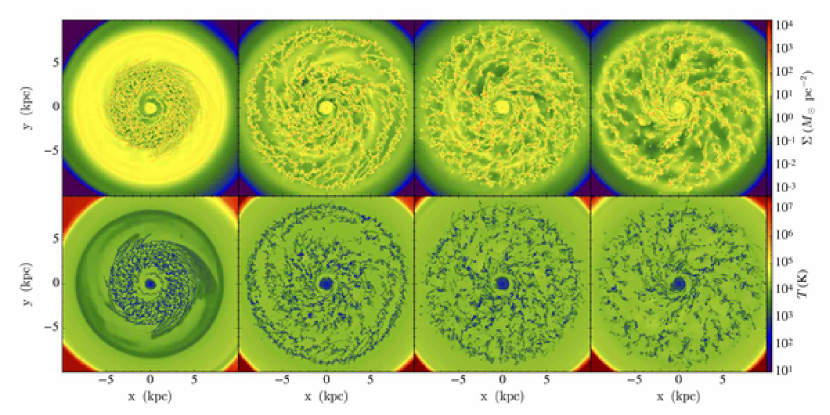
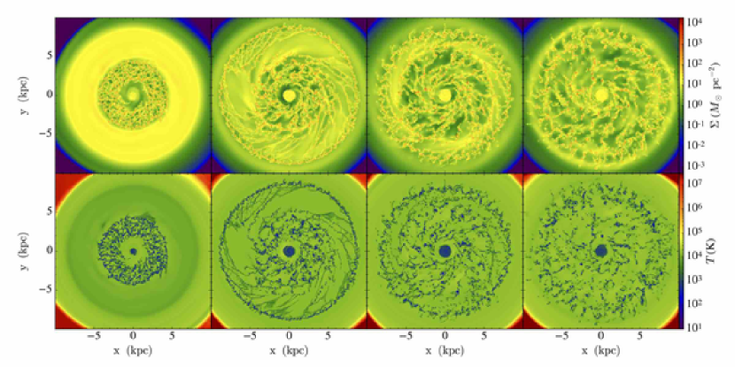
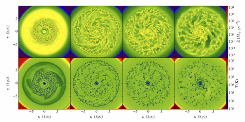
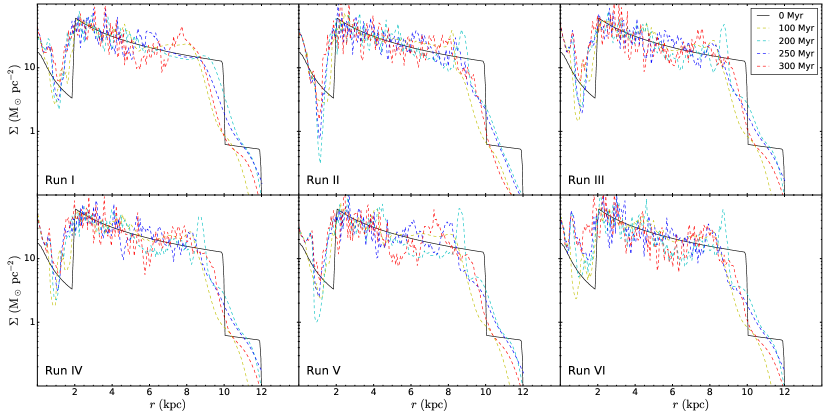
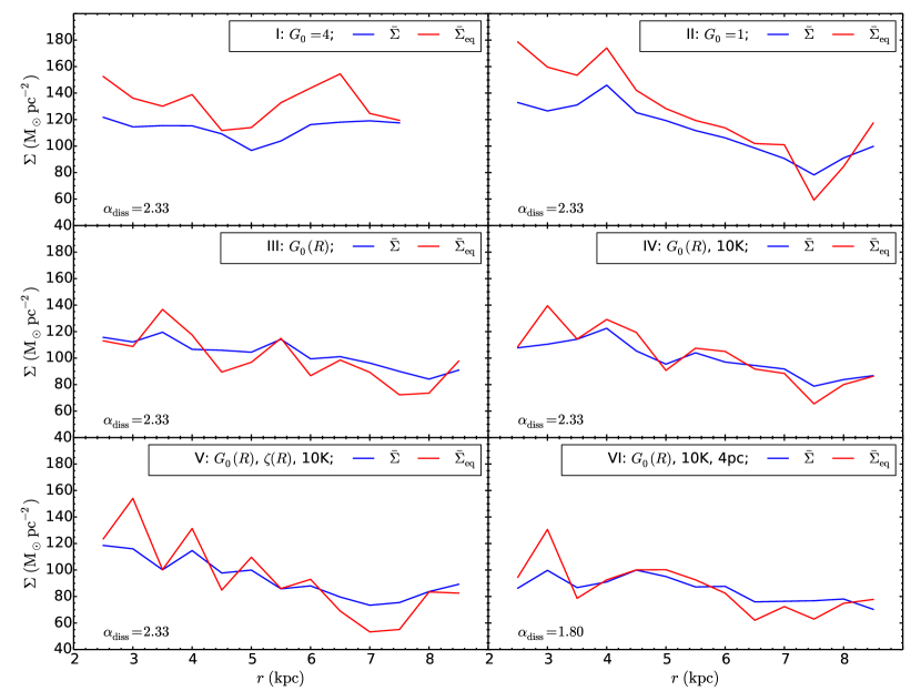
Figure 7 shows the time evolution of the radial profiles of $\Sigma$, azimuthally-averaged in annuli, in these simulations. Fluctuations on the order of factors of a few are seen to develop due to gravitational instabilities. However, overall the average values remain similar to those of the initial conditions, with the exceptions being caused by modest amounts of radial accretion seen most obviously at the boundaries of the main disk region. These results are relatively insensitive to the choices of PDR-related parameters.

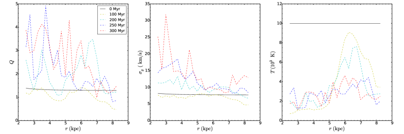
The time evolution of the azimuthally-averaged radial profiles (in range 2.5 kpc$<r<$ 8.5 kpc, with annuli of width 0.5 kpc) of the Toomre $Q$ parameter, the 1D gas velocity dispersion $\sigma_{g}$, and average gas temperature $T$ for Run VI are shown in Figure 8. Note that $\sigma_{g}=\sqrt{c_{s}^{2}+\sigma^{2}_{\rm nt}}$ is a mass-weighted average over -1 kpc$<z<$ 1 kpc, where $\sigma_{\rm nt}$ is the 1D velocity dispersion of the gas motions in the plane of the disk after the subtraction of the local circular velocity, $T$ is a mass-weighted average over -1 kpc$<z<$ 1 kpc and $Q$ is calculated via

$$Q=\frac{\kappa\sigma_{g}}{\pi G\Sigma}.$$ (7)

During the early stage of the simulation, the gas cools rapidly, causing $Q$ to drop and leading to gravitational instability. The inner region, where gas is denser, has faster cooling, so GMCs form earlier. We will see below that disk fragmentation eventually (by $\sim 200\>$Myr) reaches a relatively steady state, with the ISM existing in two main phases. The diffuse gas, being more exposed to the FUV field, retains a relatively high temperature and so the overall mass-weighted temperature is $\gtrsim 2,000\>$K, even though the majority ($\sim 2/3$) of the mass is in dense, “GMC”-like structures. However, $\sigma_{g}$ is dominated by the random motions of GMCs in the disk, i.e., $\sigma_{\rm nt}$. These are accelerated by mutual gravitational interactions between self-gravitating GMCs and damped by cloud-cloud collisions (Gammie et al. 1991). Thus at late times, $Q$, as defined by equation (7), rises to values of $\sim 3$, i.e., it is already in a highly fragmented state due to gravitational instability, but then has the superficial appearance of being gravitationally stable.

Figure 8: Galactic disk azimuthally averaged radial profiles (2.5 kpc$<r<$ 8.5 kpc) and their evolution for Run VI; from left to right: (a) Toomre $Q$ parameter, (b) one-dimensional gas velocity dispersion, $\sigma_{g}$ (mass-weighted average over -1 kpc$<z<$ 1 kpc), (c) gas temperature (mass-weighted average over -1 kpc$<z<$ 1 kpc).

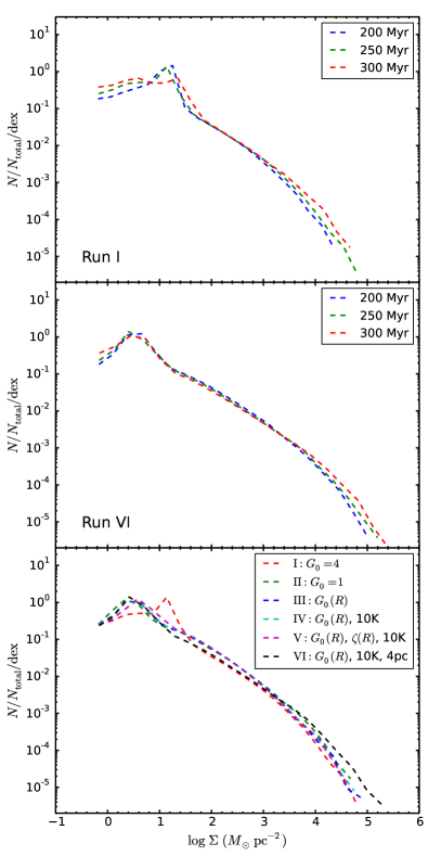
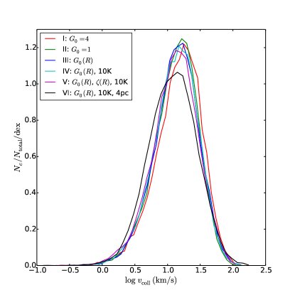
The top panel of Figure 9 shows the evolution of the $\Sigma$ PDF of Run I from 200 to 300 Myr. Overall this PDF stays relatively constant during this period, implying that the ISM of the global disk is approaching a quasi statistical equilibrium. However, there is a tendency seen for the mass fraction in the densest regions to be increasing. The effect of the final spreading of fragmentation to the outer disk by 300 Myr is also apparent in reducing the peak near $\Sigma=10\>M_{\odot}\>{\rm pc}^{-2}$. The middle panel shows equivalent results for Run VI, which is closer to full fragmentation during the period from 200 to 300 Myr. These PDFs show a greater degree of constancy, with just a minor enhancement in the fraction of material at the highest mass surface densities as the disk evolves. However, examining the morphologies shown in Fig. 6 we do see a trend for apparent agglomeration of clouds into larger structures. This will be examined further in terms of GMC mass functions in the next section. Finally, the bottom panel of Figure 9 compares the $\Sigma$ PDFs of all six runs at 250 Myr. Overall the results are quite similar between the different runs, with the case of $G_{0}=4$ having the largest differences, as fragmentation in the outermost regions is still ongoing. The result of Run VI, which has the highest resolution, also shows a difference in being able to resolve a higher fraction of mass at the greatest mass surface densities.

Figure 9: PDFs of gas mass surface density, $\Sigma$, as viewed from above the disk, evaluated from 2.5 kpc $<\ r\ <$ 8.5 kpc and projecting through -1 kpc $<\ z\ <$ 1 kpc. Top panel: results for Run I ($G_{0}=4$) at 200 (blue), 250 (green) and 300 (red) Myr. Middle panel: results for Run VI (Variable $G_{0}$) at 200 (blue), 250 (green) and 300 (red) Myr. Bottom panel: results for Runs I (red), II (green), III (blue), IV (cyan), V (magenta) and VI (black) at 250 Myr.

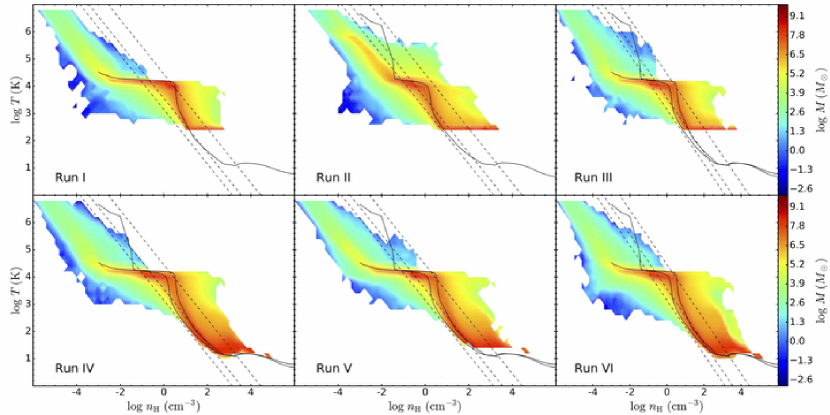
The density-temperature phase plots of the ISM at 300 Myr are shown in Figure 10 for all runs. The solid curves delineate the equilibrium temperature as a function of density, set by heating and cooling functions described in §2. Much of the mass (especially the densest parts) of the simulated ISM is at a temperature close to that expected from thermal equilibrium. Some deviations are expected due to energy injection and dissipation via dynamical processes such as heating due to compressive motions, e.g., cloud-cloud collisions, and cooling due to rarefactions.

Comparing Run IV to Run V, which has a radially variable and overall stronger $\zeta$, we can see that CR ionization is an important heating source at low temperatures ($\lesssim 30$ K), which affects the lowest temperatures that the dense gas can reach. Additionally, comparing Run IV and Run VI, one notices in the latter with its higher resolution a somewhat larger fraction of dense gas is seen to deviate from thermal equilibrium due to dynamical effects.

The typical local Milky Way total diffuse ISM pressure is about $2.8\times 10^{4}\>$K $\mathrm{cm^{-3}}$ and its thermal components are about an order of magnitude smaller (Boulares & Cox, 1990). These pressures are shown by straight lines in Figure 10. Incorporating diffuse FUV feedback, our simulated diffuse ISM has comparable thermal pressures to the observed Milky Way thermal pressures at densities $\gtrsim 10^{-1}\ \mathrm{cm^{-3}}$. At lower densities the simulation pressures are lower, which is most likely due to the lack of supernova feedback that would create a hot ionized medium with $T\gtrsim 10^{6}\>$K. At high densities, GMCs in the simulation are at much higher pressures than the diffuse ISM, mainly due to their self-gravity.

However, recall that in addition to the lack of SN feedback, the simulations also lack localized FUV, EUV and wind momentum feedback from young stars. They also lack magnetic fields and the dynamical effects due to cosmic ray pressure gradients. Both of these are important pressure components in the Milky Way. The inclusion of these physical processes is deferred to future papers in this series. Thus when interpreting the results presented here, deviations from simulated and observed ISM properties may be due to the lack of these physical processes.

Figure 10: Density versus temperature phase plots showing the distribution of gas mass at 300 Myr for Run I ($G_{0}=4$), II ($G_{0}=1$), III (radially variable $G_{0}$), IV (radially variable $G_{0}$ with 10 K temperature floor), V (radially variable $G_{0}$ and $\zeta$ with 10 K temperature floor), VI (radially variable $G_{0}$ with 10 K temperature floor and 4 pc resolution). The mass scale indicates the total mass of gas within a given $\Delta{\rm log}\>n_{\rm H}$ by $\Delta{\rm log}\>T$ interval. In each panel, the solid curves show the equilibrium temperature as a function of density. For Runs III to VI, the upper and lower solid curves at $\mathrm{n_{H}}>10^{-1.5}$ $\mathrm{cm^{-3}}$ represent the equilibrium temperature for $G_{0}=4$ and $G_{0}=1$, respectively, both with $\zeta=10^{-16}\>{\rm s}^{-1}$. The dashed lines show estimates of the total pressure in the Milky Way (Boulares & Cox 1990), $P_{\mathrm{tot}}/k=2.8\times 10^{4}\mathrm{\ K\ cm^{-3}}$ (top line), the total thermal pressure, $P_{\mathrm{th}}/k=0.36\times 10^{4}\mathrm{\ K\ cm^{-3}}$ (middle line), and the thermal pressure excluding the hot gas component, $P_{\mathrm{th,nohot}}/k=0.14\times 10^{4}\mathrm{\ K\ cm^{-3}}$ (bottom line).

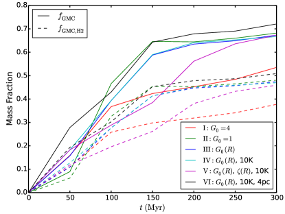
We evaluate gas density distributions and compositions for the main region of interest of the disk (2.5 kpc $<\ r\ <$ 8.5 kpc and -1 kpc $<\ z\ <$ 1 kpc). The mass fraction of gas that is in GMCs (i.e., with $n_{\rm H}\geq 100\>{\rm cm^{-3}}$), $f_{\rm GMC}$, is shown as a function of time in Figure 11 (solid lines). These fractions rise for the first $\sim 150$ Myr and then approximately stabilize. The case with $G_{0}=4$ has the smallest fraction of gas in GMCs, about 45% from 200 to 300 Myr. The other models have higher fractions, which are also very similar to each other, i.e., with about 67% of gas mass in GMCs. We note that this fraction is also very similar to that found by TT09, even though this simulation did not include FUV feedback. This tells us that the formation of dense gas, driven by gravitational instability, is not that sensitive to FUV feedback, until $G_{0}\sim 4$, when the outer disk begins to be stabilized.

Figure 11 also shows the fraction of the total gas in the disk that is in GMCs and also in the $\rm H_{2}$ phase, $f_{\rm GMC,H2}$ (dashed lines). This is the result of our PDR modeling of the gas with densities $n_{\rm H}\geq 100\>{\rm cm^{-3}}$. This fraction rises with a similar time dependence as $f_{\rm GMC}$. The ratio of the dashed and solid lines for a given simulation, i.e., $f_{\rm GMC,H2}/f_{\rm GMC}$, is the average $\rm H_{2}$ mass fraction within our defined “GMCs.” We see that this ratio is close to 70%. This is broadly consistent with the fact that Galactic GMCs are known to have large mass fractions in atomic envelopes (Blitz (1990); Wannier et al. (1991)). Thus our choice of $n_{\rm H}=100\>{\rm cm^{-3}}$ as a threshold density to define “GMCs” appears reasonable.

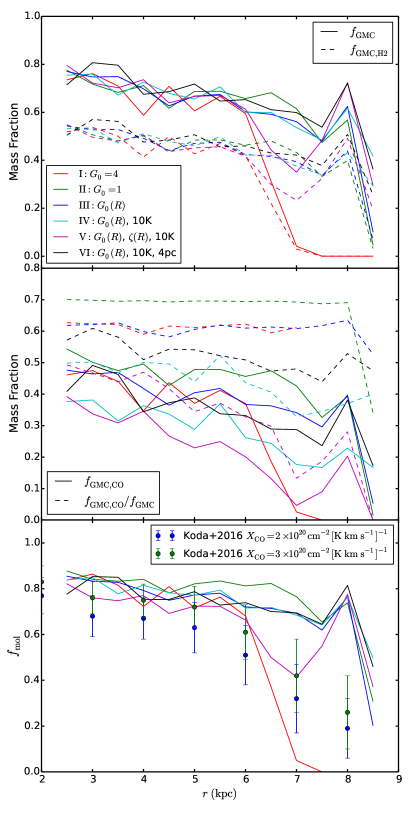
Figure 12a shows the radial profiles of $f_{\rm GMC}$ and $f_{\rm GMC,H2}$ at 250 Myr. These fractions decline gradually as one goes from the denser, inner regions to the lower density, outer regions of the disk. In Run I, i.e., with high $G_{0}$, the transition from a gravitationally unstable inner ($\lesssim 6.5\>$kpc) zone to a stable outer region is clearly seen in these profiles. The other simulation runs are seen to have radial profiles of these metrics that are quite similar to each other.

In Figure 12b with solid lines, we show the galactic radial profiles at 250 Myr of the fraction, $f_{\rm GMC,CO}$, of the total disk mass that is in “GMCs” and has a CO abundance $n_{\rm CO}/n_{\rm H}>10^{-5}$, i.e., within an order of magnitude of the maximal CO abundance of $n_{\rm CO}/n_{\rm H}=10^{-4}$, given our adopted total C and O abundances (i.e., $n_{\rm C}/n_{\rm H}=1\times 10^{-4}$). Like $f_{\rm GMC}$ and $f_{\rm GMC,H2}$, the profiles of $f_{\rm GMC,CO}$ show a general decrease with $r$, but now starting from values of $\sim 0.5$ in the inner disk and reaching $\sim 0.1$ (or less in the case of Run I) in the outer disk. As expected, Run II with a low value of $G_{0}=1$ has the highest values of $f_{\rm GMC,CO}$. Run V, with overall strongest CR ionization rate, generally shows the lowest $f_{\rm GMC,CO}$, which we attribute to the fact that CO is efficiently destroyed indirectly by CRs via creation of He⁺ (Bisbas et al., 2015). Figure 12b also shows the ratio $f_{\rm GMC,CO}/f_{\rm GMC}$ (dashed lines), which represents how well CO traces the defined “GMCs.” Comparing the first three runs, a stronger FUV radiation leads to slightly lower values of $f_{\rm GMC,CO}/f_{\rm GMC}$. Here we again see that higher values of CRs in Run V compared to Run IV over most of the disk lead to reduced fraction of the GMCs that are well traced by CO. In general, the structures identified as “GMCs” can have significant, $\sim 1/3$ mass fractions in “CO-dark” regions (and even more in Run V), consistent with the properties of Milky Way GMCs (e.g., Wolfire et al. (2010)).

Figure 12c shows the radial profile of $f_{\rm mol}\equiv\Sigma_{\rm H2}/(\Sigma_{\rm H2}+\Sigma_{\rm HI})$ in the simulations and a comparison with its observed profile in the Milky Way from the analysis of Koda et al. (2016). We see that there is generally quite good agreement between the simulations and the observational data, indicating that, at least by this metric, the simulations are a reasonable representation of the Milky Way, and perhaps indicating that various physical effects that are not yet included (e.g., localized star formation feedback, including supernovae), are not that important in regulating molecular mass fractions.

To gauge if the ISM of the main disk region achieves a quasi statistical equilibrium state from 200 to 300 Myr, Table 3.1 summarizes the values of $f_{\rm GMC}$ and $f_{\rm GMC,H2}$. We see that in most runs the ISM is in a relatively steady state during this period, with little ($\lesssim 10\%$) change in these metrics. However, runs I ($G_{0}=4$) and V (variable $G_{0}$ and $\zeta$) are a little different, since the fragmentation of outer disk regions is delayed and is continuing even after 200 Myr. Thus from 200 to 300 Myr, $f_{\rm GMC}$ increases by about 20% in these runs. Table 3.1 also shows the fractions of the total $\mathrm{H}_{2}$ mass in the main disk region that are contained in the defined GMCs, i.e., $M_{\mathrm{GMC,\mathrm{H2}}}/M_{\mathrm{disk,\mathrm{H2}}}$. These fractions are typically $>80\%$. We also list the fractions, $f_{\rm GMC,CO}$, of the disk gas mass that is in “GMCs” and “CO-rich,” and $f_{\rm GMC,CO}/f_{\rm GMC}$. Again, these quantities are relatively stable, except for Runs I and V.

Figure 11: Fraction of total disk mass in “GMCs,” i.e., with $n_{\rm H}>100\>{\rm cm^{-3}}$ ($f_{\rm GMC}$) as a function of simulation time (solid lines) for Run I (red), II (green), III (blue), IV (cyan), V (magenta) and VI (black). The dashed lines show the fraction of the total disk mass that is in “GMCs” and is in the $\rm H_{2}$ phase ($f_{\rm GMC,H2}$).

Properties of the ISM at 200 and 300 Myr are shown for each simulation run. From left to right: mass fraction of total disk gas in GMCs ($f_{\rm GMC}$); mass fraction of total disk gas in GMCs and in the $\mathrm{H_{2}}$ phase ($f_{\rm GMC,H2}$); $f_{\rm GMC,H2}/f_{\rm GMC}$; GMC $\mathrm{H_{2}}$ phase mass compared to the whole disk’s $\mathrm{H_{2}}$ mass; mass fraction of total disk gas in GMCs that is also “CO rich,” i.e., with $\mathrm{n_{CO}/n_{H}>10^{-5}}$ ($f_{\rm GMC,CO}$); mass fraction of GMC gas that is “CO rich,” i.e., $f_{\rm GMC,CO}/f_{\rm GMC}$. Run $f_{\rm GMC}$ $f_{\rm GMC,H2}$ $f_{\rm GMC,H2}/f_{\rm GMC}$ $M_{\mathrm{GMC,\mathrm{H2}}}/M_{\mathrm{disk,\mathrm{H2}}}$ $f_{\rm GMC,CO}$ $f_{\rm GMC,CO}/f_{\rm GMC}$ Time (Myr) 200 300 200 300 200 300 200 300 200 300 200 300 I 0.452 0.535 0.319 0.377 0.706 0.705 0.857 0.859 0.395 0.468 0.874 0.875 II 0.644 0.682 0.467 0.478 0.706 0.714 0.791 0.814 0.634 0.673 0.984 0.987 III 0.634 0.673 0.447 0.474 0.705 0.704 0.844 0.847 0.547 0.597 0.863 0.887 IV 0.641 0.667 0.450 0.469 0.702 0.703 0.840 0.839 0.382 0.456 0.596 0.684 V 0.561 0.672 0.381 0.459 0.680 0.683 0.890 0.889 0.177 0.388 0.316 0.577 VI 0.678 0.721 0.479 0.509 0.706 0.706 0.897 0.901 0.500 0.576 0.737 0.799

Figure 12: (a) Top panel: Fraction of total disk gas mass in “GMCs” ($f_{\rm GMC}$), i.e., with $n_{\rm H}>100\>{\rm cm^{-3}}$, as a function of galactocentric radius (solid lines) for Runs I to VI as indicated in legend, all evaluated at 250 Myr. The dashed lines show the fraction of the total disk gas mass in the “GMCs” that is also in the $\rm H_{2}$ phase ($f_{\rm GMC,H2}$). (b) Middle panel: Fraction of total disk gas mass in GMCs that is also “CO-rich,” i.e., with $n_{\rm CO}/n_{\rm H}>10^{-5}$ ($f_{\rm GMC,CO}$ - solid lines), with results shown for the runs at 250 Myr (see legend in panel a). The ratio $f_{\rm GMC,CO}/f_{\rm GMC}$ is also shown (dashed lines). (c) Bottom panel: Molecular fraction, $f_{\rm mol}\equiv\Sigma_{\rm H2}/(\Sigma_{\rm H2}+\Sigma_{\rm HI})$ for the different runs (see legend in panel a), compared to the Milky Way from the analysis of Koda et al. (2016) for two different values of $X_{\rm CO}$, as indicated.

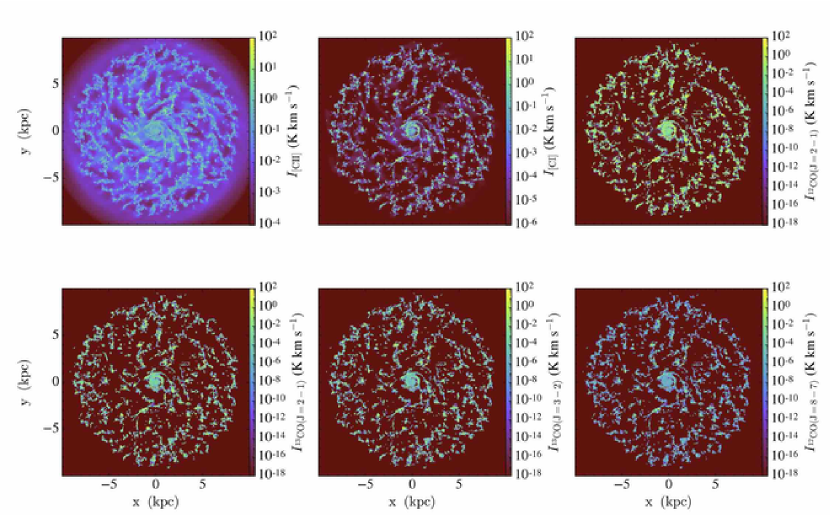
In Figure 13 we show several diagnostic tracers of the global disk of Run VI at 250 Myr: [CII] 158 $\mathrm{\mu m}$, CI 609 $\mathrm{\mu m}$, ¹²CO($J$ = 2–1), ¹³CO($J$ = 2–1), ¹³CO($J$ = 3–2) and ¹²CO($J$ = 8–7). Note that the adopted abundance ratio of ¹³C to ¹²C is 1/60. In constructing these maps we have simply summed the local emissivities and not accounted for optical depth. However, such optical depth effects are partially accounted for in the local 1D PDR models. This will mostly affect the ¹²CO(2-1) results, which should be regarded as illustrative and not meant for quantitative assessment of line intensities. However, the other CO tracers are expected to be closer to being optically thin and thus more accurately represented by these maps.

As expected, the [CII] 158 $\mathrm{\mu m}$ emission is much more diffuse than the CO emission, i.e., tracing not only the cooler, denser structures, but also warmer and lower density regions ($n_{\mathrm{H}}\sim$10 – 100 ${\rm cm^{-3}}$) that are near the transition from the atomic to molecular phase. We see that CO emission lines are emitted from much more discrete, localized clouds. ¹²CO($J$ = 2–1), ¹³CO($J$ = 2–1) and ¹³CO($J$ = 3–2) intensity maps show similar structures. On the scales shown in Figure 13, ¹²CO($J$ = 8–7) also shows similar morphologies, but with lower overall intensities.

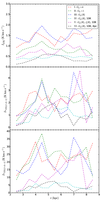
Figure 14 shows the area-weighted integrated [CII] (top panel), ¹³CO($J$ = 2–1) (middle panel) and ¹²CO($J$ = 2–1) (bottom panel) line intensities along the line of sight as functions of galactocentric radii for face-on views of the disks at 250 Myr. Comparing runs with the same temperature floor we can see that, overall, a stronger FUV radiation field leads to higher [CII] intensities, but has less influence on CO lines because it attenuates significantly through the dense regions where CO lines are strong.

Figure 13: The galactic disk for Run VI (radially variable $G_{0}$, constant $\zeta$, 4-pc resolution) at 250 Myr. Images are 20 kpc across. From top left to bottom right are shown integrated intensity maps of: (a) [CII] 158 $\mathrm{\mu m}$; (b) CI 609 $\mathrm{\mu m}$; (c) ¹²CO($J$=2–1); (d) ¹³CO($J$=2–1); (e) ¹³CO($J$=3–2); (f) ¹²CO($J$=8–7).

Figure 14: Area-weighted integrated [CII] 158 $\mathrm{\mu m}$ (top panel), ¹³CO($J$ = 2–1) (middle panel) and ¹²CO($J$ = 2–1) (bottom panel) emission line intensities along the line of sight as a function of galactocentric radii for face-on views of the disks of Run I (red), II (green), III (blue), IV (cyan), V (magenta), VI (black) (all results for $t=250\>$Myr).

3.2 Example Kiloparsec Patches

To examine the structure of the ISM on scales $\lesssim 1\>$kpc, we extract example 1 kpc disk patches from the simulations at galactocentric radius of 4.25 kpc and at 250 Myr and visualize their mass surface density and temperature structures in Figure 15. These are the locations and times extracted from the TT09 simulation and used as initial conditions for higher resolution simulations by Van Loo et al. (2013, 2015), Butler et al. (2015) and Butler et al. (2017).

The patches show large variations from run to run, which is caused by the chaotic nature of small scale ISM, including GMC, evolution. General features include the presence of elongated, filamentary structures, some of which may be related to tidal tails around denser clouds. In the patches where there are high numbers of dense clouds, there is clear evidence for interactions.

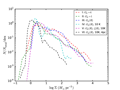
The probability distribution functions (PDFs) of mass surface density (calculated with a fixed linear resolution, 8 pc for Runs I to V and 4pc for Run VI) are shown in Figure 16. Again, these show a variety of shapes, but generally peak at few $M_{\odot}\>{\rm pc}^{-2}$, with high-end power law tails. A great deal of variation is due simply to stochastic sampling within a galaxy: for example, the region extracted from Run VI only has a couple of small GMCs and so has the smallest areal fraction of material above, e.g., $10\>M_{\odot}\>{\rm pc}^{-2}$.

Figure 15: (a) Top row: The mass surface density structures of 1-kpc-wide patches of the disks (averaged vertically over a 2 kpc vertical extent centered on disk midplane) centered at $(x,y)=(4.25,0)$ kpc at 250 Myr, extracted from Runs I to VI (left to right). This part of the disk is in a quasi-steady state at this time with respect to the distribution of ISM phases for all these simulation runs, but large variations still occur on $\sim$kpc scales. (b) Bottom row: As (a), but now showing mass-weighted temperature.

Figure 16: Probability distribution function (PDF) of gas mass surface density evaluated in the 1 kpc patch regions centered at $(x,y)=(4.25,0)$ pc at 250 Myr for Runs I (red), II (green), III (blue), III (blue), IV (cyan), V (magenta) and VI (black).

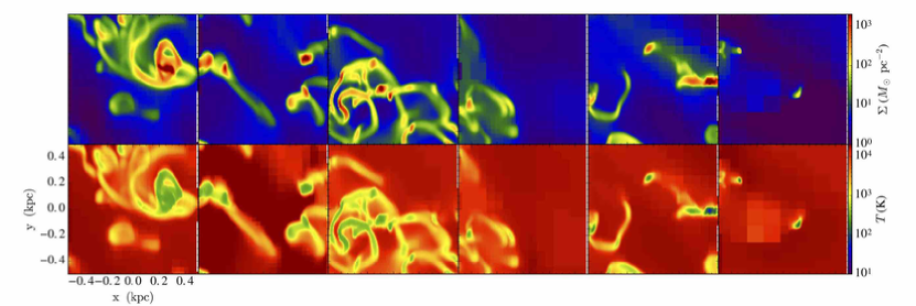
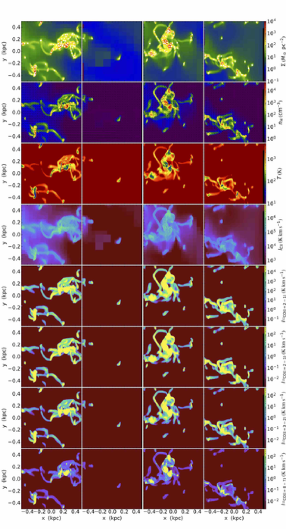
We also display a series of kiloparsec patches from Run VI, centering at $r=3$, 4.25, 5.25 and 7 kpc (Figure 17). These regions contain a great variety of structures, as seen in their mass surface densities, mass-weighted number densities and temperatures, and integrated intensities of emission lines [CII] 158 $\mathrm{\mu m}$, ¹²CO($J$=2–1), ¹³CO($J$=2–1), ¹³CO($J$=3–2) and ¹²CO($J$=8–7) along the line of sight ($z$-direction). Here in the $\Sigma$ map we also show the center of mass locations of identified “GMCs.” As noted earlier, [CII] 158 $\mathrm{\mu m}$ line emission, tracing warmer and lower density ($n_{\mathrm{H}}\sim$10–100${\rm cm^{-3}}$) gas, is much more diffuse and extended than that of CO lines.

In principle, the statistics of line and dust continuum emission from ensembles of such kpc patches, or whole galaxies, may be compared to observations of nearby galaxies, e.g., with ALMA or SOFIA. Such data could first be used to constrain a global model for a galactic disk (e.g., rotation curve, total gas $\Sigma(r)$ profile), then allowing a tailored simulation of a particular system. Then the detailed statistics of the distributions of emissivities could be used to test the validity of the simulations, e.g., comparing the effects of including $B$-fields and/or methods of implementing feedback. Such comparisons are are a longer term goal of this project.

Figure 17: Examples of 1 kpc sized patches (integrated over 2 kpc in the $z$-direction), extracted from the main disk of Run VI at 250 Myr, centering at $r=3$, 4.25, 5.25, and 7 kpc (columns from left to right) in the mid plane. Rows from top to bottom show the total gas mass surface density ($\Sigma$), mass-weighted number density of H nuclei ($n_{\rm H}$), mass-weighted temperature ($T$), and integrated [CII] 158 $\mathrm{\mu m}$, ¹²CO($J$=2–1), ¹³CO($J$=2–1), ¹³CO($J$=3–2) and ¹²CO($J$=8–7) line intensities. The center of mass of identified clouds are marked as white points in the top row, which also shows the local velocity field, i.e., after subtracting the mean circular orbital velocity at each location.

4 GMC Physical Properties

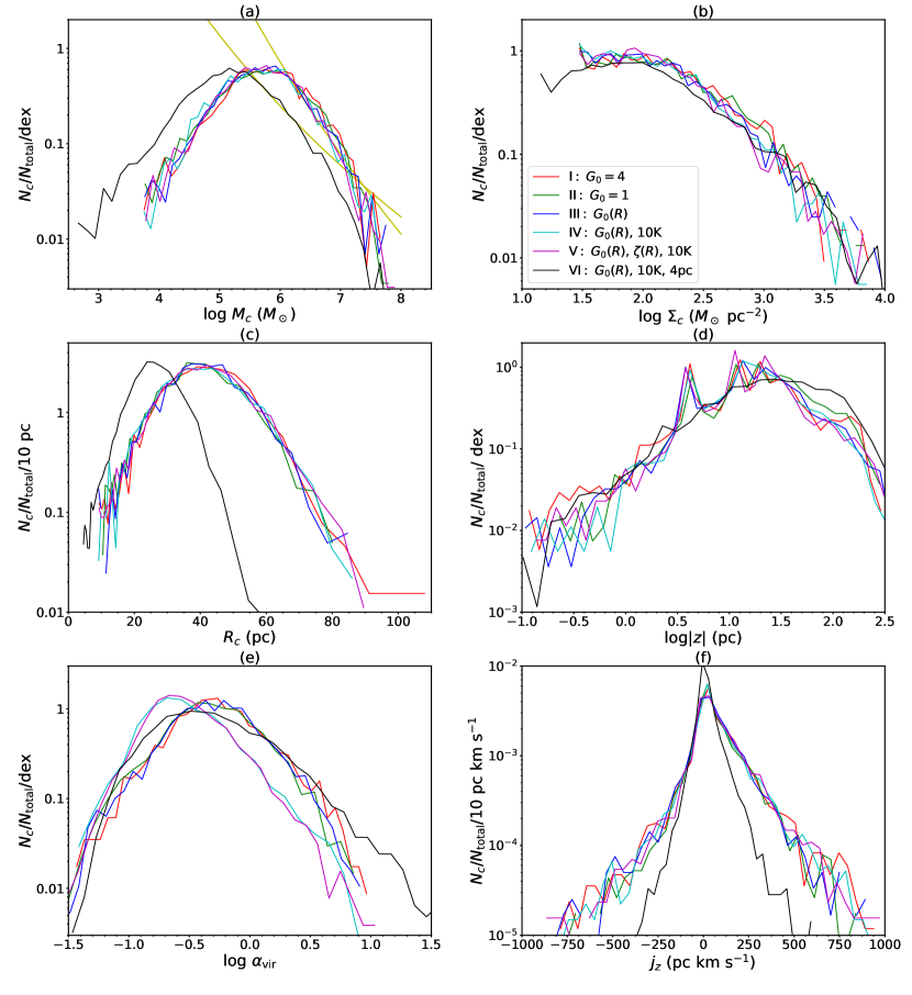
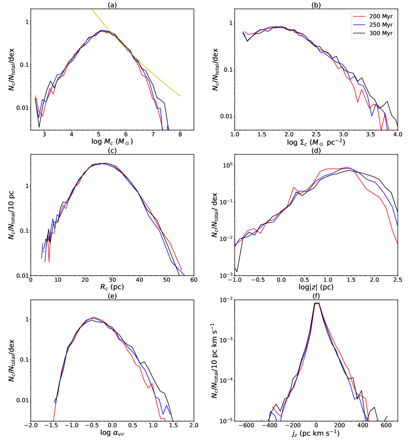
In this section we show the physical properties of the identified “GMCs,” which, recall, are connected, locally-peaked structures identified by having $n_{\rm H}\geq 100\>{\rm cm}^{-3}$ (see §2). Our analysis methods follow those of TT09. We focus on GMC properties during the period from 200 to 300 Myrs when the disks are in quasi-statistical equilibrium in terms of their global ISM properties, as shown in the previous section. Figure 18 compares the probability distribution functions (PDFs) of several GMC properties for all six runs at 300 Myr. Figure 19 presents the time evolution of these PDFs from 200 to 300 Myr for Run VI.

GMC mass ($M_{c}$) PDFs are shown in Figure 18(a). For Runs I to V (i.e., with 8 pc resolution), these PDFs show a broad peak near $5\times 10^{5}\>M_{\odot}$, with clouds seen with masses from $\sim 10^{4}\>M_{\odot}$ to $\sim 5\times 10^{7}\>M_{\odot}$. We see that these GMC mass functions are fairly insensitive to the modeled PDR and CR physics. However, the linear resolution of the simulation has a significant effect: i.e., Run VI has a GMC mass function that peaks at lower masses. We fit power laws of the form $\mathrm{d}N_{c}/\mathrm{d}\>{\rm log}\>M_{c}\propto M_{c}^{-\alpha}$ to the high-end range ($>10^{6}\>M_{\odot}$ for Runs I to V; $>10^{5.5}\>M_{\odot}$ for Run VI), with errors set from Poisson counting statistics in each mass interval. Runs I to V have values of $\alpha\simeq 1.4$, while Run VI has $\alpha\simeq 0.93\pm 0.03$. Thus we see that the resolution of the simulation has a significant effect on the mass function of the GMCs, as defined with our selection criteria of §2. Note that our selection of GMCs in Run VI uses the same deblending distance parameter of 32 pc as the other runs, so the difference in the mass function arises because of Run VI’s ability to better resolve fragmentation of the structures.

Figure 19(a) shows that the GMC mass function remains very constant from 200 to 300 Myr for Run VI, with the most noticeable evolution being a small increase in the number of the most massive clouds by the time of 300 Myr. As discussed earlier, detailed results of GMC mass functions are likely influenced by the lack of localized star formation and feedback in these simulations, since diffuse FUV feedback on its own is ineffective at destroying GMCs. However, since the mass fraction of gas in GMCs is quite stable (§3), we hypothsize that in these simulations it is the process of GMC collisions that act to regulate the GMC population, i.e., keeping $\sim 1/3$ of the gas in the diffuse intercloud medium.

Figure 18: Probability distribution functions (PDFs) of GMC properties for Runs I (red), II (green), III (blue), IV (cyan), V (magenta) and VI (black) at 300 Myr (see legend). The panels show: (a) mass; (b) mass surface density; (c) average radius; (d) center-of-mass vertical position; (e) virial parameter; (f) specific angular momenta. The straight yellow lines in (a) show power law fits to the high-end GMC mass spectra $\mathrm{d}N_{c}/\mathrm{d}\>{\rm log}\>M_{c}\propto M_{c}^{-\alpha}$ with $\alpha=1.43\pm 0.08$ and $0.93\pm 0.03$ for Run IV and VI, respectively, at 300 Myr (see text).

Figure 19: As Figure 18, but now showing results for Run VI at 200, 250 and 300 Myr. The panels show: (a) mass; (b) mass surface density; (c) average radius; (d) center-of-mass vertical position; (e) virial parameter; (f) specific angular momenta. The straight yellow line in (a) show a power law fit to the high-end GMC mass spectrum $\mathrm{d}N_{c}/\mathrm{d}\>{\rm log}\>M_{c}\propto M_{c}^{-\alpha}$ with $\alpha=0.93$ at 300 Myr.

We can compare the simulated GMC mass distributions to those observed in the Milky Way and M33, which can also be fitted with a power law at their high-mass end. In the Milky Way, $\alpha$ is estimated to be $\sim 0.6-0.8$ (Williams & McKee, 1997), based on analysis of ¹²CO(1-0) line survey data. In the inner ($\leq 2\>$kpc) region of M33, with $\sim 50\>$pc resolution, Gratier et al. (2012) measure $\alpha\simeq 0.6\pm 0.2$ (assuming a one to one correspondence of CO(2-1) line luminosity with GMC mass). At galactocentric distances $>2\>$kpc, they measure $\alpha\simeq 1.3\pm 0.2$. While the values of $\alpha$ seen in Run VI (i.e., $\alpha\simeq 0.93\pm 0.03$) are similar to the above observed values, we caution that the numerical results are not converged (i.e., with the 4 pc resolution of Run VI, we see a much shallower high-end power law slope). At the same time, one must recognize that observational results will also likely depend on the linear resolution achieved and the particular method of GMC identification and mass measurement. Most observational studies of GMC mass functions use ¹²CO line emission to identify the clouds, followed by empirical relations to convert line luminosities to mass. Since our PDR modeling does not yet include accurate treatment of the global radiative transfer effects that are important for the fluxes of optically thick lines, like ¹²CO(2-1), we defer more detailed comparisons of the GMC mass (and line luminosity) functions to a future paper.

Figure 18(b) shows the distributions of mass surface densities, $\Sigma_{c}\equiv M_{c}/(\pi R_{c}^{2})$, of the clouds as viewed along the $z$-axis, perpendicular to the disk, at 300 Myr. Here $R_{c}$ is the average projected radius of the GMCs in the disk plane, discussed below. The distributions of mass surface densities are very similar among the six runs, with a broad peak near $\sim 60\>M_{\odot}\>{\rm pc}^{-2}$ (the peak becomes most apparent in Run VI), which falls off with a power law tail at the high $\Sigma$ end. The minimum value of $\Sigma_{c}$ can be understood as simply being related to that of a GMC which is only resolved with a single layer of grid cells in the vertical direction: i.e., $\simeq 28\>M_{\odot}\>{\rm pc}^{-2}$ for an 8 pc sided cell filled with gas at $n_{\rm H}=100\>{\rm cm}^{-3}$ and half this value for the 4 pc resolution Run VI. On the otherhand, a few, extreme “GMCs” have $\Sigma\sim 10^{4}\>M_{\odot}\>{\rm pc}^{-2}$. Figure 19(b) shows that the PDFs of $\Sigma$ for Run VI remain quite constant from 200 to 300 Myr. There is slight growth in the high-$\Sigma$ tail of the distribution, but this involves only a relatively small number of clouds.

The mass surface density of the peak of the PDF of the Run VI GMCs is similar to the mean value of $\sim 200\>M_{\odot}\>\mathrm{pc}^{-2}$ derived by Solomon et al. (1987) from a ¹²CO(1-0) survey of the Galaxy. Heyer et al. (2009) have derived smaller values $\sim 100M_{\odot}$ $\mathrm{pc}^{-2}$ based on better sampled ¹³CO surveys (see discussion of Tan, Shaske & Van Loo 2013). Considering the difference in GMC identifications between observations based solely on molecular line (CO) emission, and our simulated clouds, $\Sigma$ values of our simulated GMCs are broadly consistent with observations. Nevertheless, we again expect that additional physics of $B$-fields, star formation and localized feedback will all act to reduce $\Sigma$ of the GMC population.

Figure 18(c) shows the PDFs of average GMC radius, $R_{c}\equiv(A_{c}/\pi)^{1/2}$, where $A_{c}$ is the projected area viewed along the $z$ axis. Given the results for the PDFs of $M_{c}$ and $\Sigma_{c}$, the similarity of the PDFs among Runs I to V is not surprising. Their PDFs peak at $R_{c}\simeq 40\>$pc, then extending up to $\sim 100\>$pc. For Run VI, the peak of the PDF is near $25\>$pc and the largest GMCs have radii of $\sim 50\>$pc. Figure 19(c) shows the constancy of the $R_{c}$ distribution from 200 to 300 Myr for Run VI. These results show that the sizes of identified “GMCs” depend on the resolution of the simulation and are thus not numerically converged. Still, the sizes of the clouds in Run VI are comparable to those observed for GMCs in the Galaxy (e.g. Miville-Deschênes et al. (2017)).

Figure 18(d) shows the distribution of the magnitudes of the vertical distances of GMC center of masses from the disk midplane. Most clouds are located within a narrow range of $\sim 30$ pc from the midplane. The vertical half-scale-height of the population of GMCs is $|z|_{1/2}=26\>$pc, i.e., the median value of $|z|$. This half-scale-height is similar to the typical radii of the GMCs, demonstrating that the GMCs interact as part of a quasi-2D distribution, which is an assumption of the GMC-GMC collision models of Gammie et al. (1991) and Tan (2000), discussed below. A small number of GMCs are at relatively large vertical displacements from the midplane. Figure 19(d) shows the numbers of these high $|z|$ GMCs increases moderately from 200 to 300 Myr in Run VI. All vertical displacements of the GMCs in these simulations are driven by gravitational forces acting between the self-gravitating clouds. Generally the largest velocities that will be achieved in such interactions will be approximately equal to the escape speed from the clouds. As shown in Fig. 8(b), the gas velocity dispersion in the disk plane can reach 30 km/s at late times in the inner region of the galaxy. A larger range of $|z|$ at later times is consistent with the growth of some GMCs to larger masses and higher densities, as discussed above.

Figure 18(e) shows the distribution of GMC virial parameters, defined as (Bertoldi & McKee, 1992)

$$\alpha_{\rm vir}\equiv\frac{5\sigma_{c}^{2}R_{c}}{GM_{c}},$$ (8)

where $\sigma_{c}$ is the mass-averaged 1D velocity dispersion of the cloud, i.e., $\sigma_{c}\equiv(c_{s}^{2}+\sigma^{2}_{\mathrm{nt},c})^{1/2}$ and $\sigma^{2}_{\mathrm{nt},c}$ is the 1D velocity dispersion about the center-of-mass velocity of the cloud. A value of $\alpha_{\rm vir}=1$ implies a spherical, uniform cloud with negligible surface pressure and magnetic fields is virialized, while $\alpha_{\rm vir}<2$ indicates this type of cloud is gravitationally bound. The PDFs of $\alpha_{\rm vir}$ are relatively broad, but tending to peak at values $<1$. The effect of the 300 K temperature floor is clearly seen in Runs I, II and III, since it sets an effective minimum velocity dispersion of about 1.6 km/s. Runs IV and V have PDFs of $\alpha_{\rm vir}$ that peak at significantly lower values. Interestingly, the distribution of $\alpha_{\rm vir}$ rises again in the GMCs in the higher resolution simulation Run VI. Figure 19 shows this distribution remains nearly constant from 200 to 300 Myr. At 300 Myr, its median value is $\alpha_{\rm vir}\simeq 0.45$. Most (78%) of the GMCs are gravitationally bound, consistent with the observational results of Roman-Duval et al. (2010), as analyzed by Tan et al. (2013). GMCs that are unbound are likely due to the dynamical effects of strong gravitational interactions, including recent collisions, between GMCs.

Figure 18(f) shows the distribution of GMC specific angular momenta about a rotation axis through the center of mass perpendicular to the disk plane, i.e., $j_{z}$. Positive values of $j_{z}$ indicate prograde rotation, i.e., in the same sense as the orbital motion of the galaxy, while negative values indicate retrograde rotation. The distributions are similar among Runs I to V, showing a modest excess of prograde over retrograde GMCs. The fraction of retrograde GMCs is $f_{\rm retro}\simeq 0.28$ for these GMC populations. The distrbution in Run VI is narrower, as expected since GMCs are smaller, and its value of $f_{\rm retro}\simeq 0.36$ is slightly greater than the results of the other runs. Figure 19(f) shows that the Run VI PDF of $j_{z}$ does not change significantly during the period from 200 to 300 Myr. As discussed by TT09 (see also Dobbs (2008); Dobbs et al. (2011)), $f_{\rm retro}$ may be a useful diagnostic of the role of GMC-GMC collisions in a galaxy population. Large values of $f_{\rm retro}$ may indicate that GMCs are collisionally evolved. Our results are consistent with observations showing that retrograde clouds are nearly as common as prograde ones (Blitz (1993); Phillips (1999); Rosolowsky et al. (2003); Imara & Blitz (2011); Imara et al. (2011)).

5 GMC Collisions

Shear-driven GMC-GMC collisions have been proposed as a mechanism to trigger star cluster formation, which could then explain the SFRs of disk galaxies and circumnuclear starbursts (Tan (2000); see also TT09; Tan (2010); Tan et al. (2013); Suwannajak et al. (2014)). This model assumes the galactic disk has a Toomre parameter $Q\sim 1$ and a significant fraction, $f_{\rm GMC}\sim 0.5$, of its gas mass in self-gravitating clouds, i.e., “GMCs,” which occupy an essentially 2D distribution in the disk plane (i.e., the scale height of the GMCs is similar to the size of the clouds). These conditions were met by the disk simulated by TT09 and are also achieved by the new disk simulations presented in this paper. Under such conditions, gravitational interactions between GMCs lead to an increase in the velocity dispersion of the clouds, which is eventually balanced by damping by GMC collisions (Gammie et al., 1991). These “peculiar motions” of GMCs with respect to their local circular velocity cause GMCs to interact with other clouds that are on orbits with slightly different mean galactocentric radii. For a population of equal mass GMCs, typical collisions occur between clouds that have initial mean orbital separations, i.e., collision impact parameters, of $b\sim 1.6r_{t}$ with a range of $\Delta b\sim r_{t}$, where $r_{t}=(1-\beta)^{-2/3}(2M_{c}/M_{\rm gal})^{1/3}r$ is the tidal radius of the clouds, with $\beta\equiv d\>{\rm ln}\>v_{\rm circ}/d\>{\rm ln}\>r$, and $M_{\rm gal}$ is the total galactic mass interior to galactocentric radius $r$.

Under these conditions, the average rate of GMC-GMC collisions is estimated to be (Tan (2000); see also Tan et al. (2013)):

$$t_{\rm coll} \simeq \frac{1}{2}\frac{\lambda_{\rm mfp}}{v_{s}(b=1.6r_{t})}$$ (9)

$$\simeq \frac{1}{2b^{\prime}(\Omega-\mathrm{d}v_{\rm circ}/\mathrm{d}r){\cal N}_{A}r_{t}^{2}f_{G}},$$ (10)

where $\lambda_{\rm mfp}$ is the mean free path between collisions, $v_{s}$ is the shear velocity in the disk for orbits separated by a given initial impact parameter, i.e.,

$$v_{s}=b(\Omega-\mathrm{d}v_{\rm circ}/\mathrm{d}r),$$ (11)

$b^{\prime}\equiv b/r_{t}\simeq 1.6$, $\Omega=v_{\rm circ}/r=2\pi/t_{\rm orb}$, ${\cal N}_{A}$ is the number of GMCs per unit area, and $f_{G}\sim 0.5$ is the fraction of strong gravitational encounters that lead to collision. This fraction depends on the physical size of the GMCs and is somewhat uncertain. For ${\cal N}_{A}\simeq f_{\rm GMC}\Sigma_{g}/\bar{M}_{c}$ and $\sigma_{g}\simeq(G\bar{M}_{c}\kappa)^{1/3}(1.0-1.7\beta)$ (Gammie et al., 1991), we have

$$t_{\rm coll} \simeq \frac{0.15Qt_{\rm orb}}{b^{\prime}f_{\rm GMC}f_{G}(1-0.7\beta)}$$ (12)

$$\rightarrow 0.19t_{\rm orb}/f_{\rm GMC},$$ (13)

where the last evaluation is for constant $v_{\rm circ}$, i.e. $\beta=0$, and for $f_{G}=0.5$. If most star formation is initiated by GMC collisions, then this result predicts $\Sigma_{\rm SFR}\propto\Sigma_{g}\Omega(1-0.7\beta)$, i.e., a modification of the “dynamical” Kennicutt-Schmidt relation observed by Kennicutt (1998), and further tested in resolved nearby galaxies by Leroy et al. (2008), Tan (2010) and Suwannajak et al. (2014).

By tracking GMCs in global galactic disk simulations, TT09 measured $t_{\rm coll}/t_{\rm orb}$ as a function of $r$, finding typical values of $\simeq 0.2$, with a tendency for this ratio to decrease gradually with increasing $r$. GMCs with $M_{c}>10^{6}\>M_{\odot}$ had $t_{\rm coll}/t_{\rm orb}\sim 0.1$; note $t_{\rm coll}$ is the average time between collisions of these massive GMCs with all other GMCs. Note also that in the simulations there are effects of there being a range of GMC masses, as well as collective interactions, i.e., in and around GMC complexes, which are not accounted for in the simple analytic estimates that are based on idealized binary collision rates. There can also be systematic variations of ${\cal N}_{A}$ and $r_{t}$ with location in the simulated disk galaxy. To account for these, Tan et al. (2013) tested the prediction of equation (10) directly in annuli in the TT09 disk, finding good agreement: in particular, the radial gradient in $t_{\rm coll}/t_{\rm orb}$ was accounted for by systematic variations in ${\cal N}_{A}$ and $r_{t}$ (e.g., partly because of variations in the average GMC mass $\bar{M}_{c}$ with galactocentric radius), and the faster collision rate of more massive clouds due to their larger tidal radii.

In this section we carry out a similar analysis of the GMC collisions in our simulated disks, as well as examining basic properties of the collisions, including mass ratios and relative velocities. We also examine the injection rate of “turbulent momentum” into GMCs that may help explain the maintenance of their internal turbulence and thus their overall structural properties.

5.1 Mass Ratios of Colliding GMCs

Figure 20: PDFs of mass ratios of colliding GMCs in Runs I to VI from 200 to 300 Myr (solid lines; see legend). The dashed lines with corresponding colors show the PDFs of mass ratios of randomly selected pairs of GMCs.

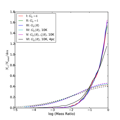
We show the PDF of mass ratios ($M_{2}/M_{1}$, where $M_{2}$ is defined as the smaller mass) of colliding GMCs in Figure 20 for Runs I to VI during the simulation time 200–300 Myr. We see that the typical mass ratio of colliding GMCs peaks close to 1 in all the simulations, i.e., collisions can be described as “major mergers.” This PDF is not a natural result of the cloud mass functions shown in Figure 18a, since the mass ratio of randomly selected pairs of GMCs is much broader (Fig. 20). Instead, it is caused by the collision rate to be higher for more massive GMCs, given their larger tidal radii.

5.2 GMC Collision Speeds

Figure 21: PDFs of relative speeds, $v_{\rm coll}$, of colliding GMCs in Runs I to VI (see legend) evaluated from 200 to 300 Myr.

The PDFs of the relative speeds $v_{\rm coll}$ of colliding GMCs are shown in Figure 21. These distributions peak at $\simeq 17\>{\rm km\>s}^{-1}$ for Runs I to V and $\simeq 13\>{\rm km\>s}^{-1}$ for Run VI. These results are consistent with the collision speeds being set by the shear velocity from encounters with initial impact parameters of $b\sim 1$ to 2 $r_{t}$, i.e., following equation (11). The smaller speeds in Run VI would then be caused by GMCs being of lower mass in this better resolved simulation. Our results are comparable to recent observations on cloud collision (e.g. Fukui et al. (2015)).

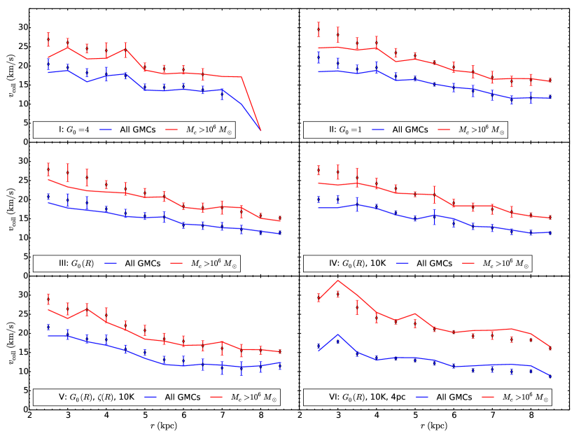
In Figure 22 we show the mean relative speed of GMC collisions as a function of galactocentric radii, averaging in annuli. The relative speed is seen to be typically a slowly decreasing function of radius, with values of $\sim 10$ to 20$\>{\rm km\>s^{-1}}$ in Run VI when averaging over all GMCs and from $\sim 15$ to 30$\>{\rm km\>s^{-1}}$ for collisions involving the $>10^{6}\>M_{\odot}$ GMCs. These results, along with those of the colliding cloud mass ratios, can help to guide the initial conditions for numerical simulations of individual cases of GMC collisions (e.g., Wu et al. (2015, 2017a, 2017b)).

We compare these speeds to the prediction of $v_{\rm coll}=v_{s}(b=1.6r_{t})$, i.e., see equation (11). This is generally accurate to within $\sim 10\%$, but does systematically underestimate the collision speed. Gravitational acceleration is expected to boost the collision speed by an amount of up to of order the free-fall speed, $v_{\rm ff}$, though geometric effects and gas pressure gradients will lower the amount of the increase. We find that a collision speed given by

$$v_{\rm coll}=v_{s}(b=1.6r_{t})+(1/6)\bar{v}_{\rm ff},$$ (14)

where $\bar{v}_{\rm ff}=(2G\bar{M}_{c}/\bar{R}_{c})^{1/2}$, gives an accurate description of the mean collision speeds in Runs I to VI and for collisions between all GMCs and for those involving GMCs with $>10^{6}\>M_{\odot}$ (see Fig. 22).

Figure 22: Average relative speeds of colliding GMCs in Runs I to VI from 200 to 300 Myr as a function of galactocentric radius. Blue solid lines show measured speeds in collisions of all GMCs; red solid lines show the speeds of collisions where one of the GMCs has a mass $>10^{6}\>M_{\odot}$. The diamonds show analytic estimates of the collision speeds following equation (14), which is based on the shear velocity at an impact parameter of $b=1.6r_{t}$ plus $\bar{v}_{\rm ff}/6$ (see text), with the error bar showing $1\sigma$ dispersion in these estimated based on GMC properties from 200 to 300 Myr.

5.3 GMC Collision Timescales

Figure 23: Cloud collision timescales (measured from 200 to 300 Myr) relative to orbital timescale as a function of galactocentric radius for Runs I to VI (panels as labelled) averaged for all GMCs (blue solid lines) and for GMCs with $M_{c}>10^{6}M_{\odot}$ (red solid lines). Diamonds show the theoretical estimates from equation 10, averaged for GMC populations from 200 to 300 Myr, with the error bars showing the $1\sigma$ standard deviation (see text).

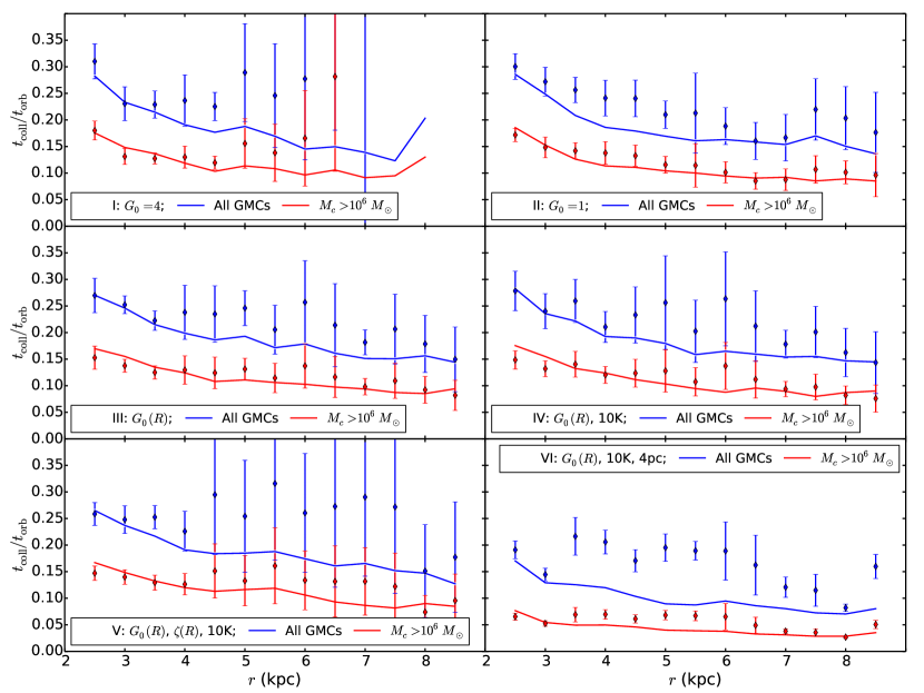
Figure 23 shows the ratio of mean GMC collision time to local orbital time, $t_{\mathrm{coll}}/t_{\rm orb}$, measured in simulation Runs I to VI from 200–300 Myr as a function of galactocentric radius averaged over all GMCs (blue lines) and for GMCs with $>10^{6}\>M_{\odot}$ (red lines). Note the local orbital time is given by

$$t_{\mathrm{orb}}=123(r/4\mathrm{\ kpc})(v_{\rm circ}/200\mathrm{km\ s^{-1}})^{-1}\ \mathrm{Myr}.$$ (15)

The average values of $t_{\mathrm{coll}}/t_{\rm orb}$ are measured by counting the total number of GMC collisions and the average total number of GMCs in annuli in the 200 to 300 Myr period, recognizing that each collision involves two GMCs, and using the value of $t_{\rm orb}$ appropriate for the middle of each annulus. We also calculate the theoretically expected value of $t_{\mathrm{coll}}/t_{\rm orb}$ based on equation (10) for $t_{\rm coll}$, which assumes $f_{G}=0.5$ and uses the number of GMCs per unit area and the mean value of GMC tidal radii, i.e., depending on $M_{c}$ and $r$, as inputs. These estimates are made for the GMC populations measured in the simulation outputs every 1 Myr from 200 to 300 Myr, with the average results shown as diamond shaped points for all GMCs (blue) and $>10^{6}\>M_{\odot}$ GMCs (red), with the vertical lines showing the $1\sigma$ dispersions.

Similar to the results of TT09 and Tan et al. (2013), the mean collision times averaged for all GMCs are seen to be a small fraction, $\sim 0.2$, of an orbital time for Runs I to V, with a gradual decline in this ratio with increasing galactocentric radius. The more massive, $>10^{6}\>M_{\odot}$ GMCs also follow this trend, but have average values of $t_{\rm coll}/t_{\rm orb}\sim 0.1$. In the higher resolution Run VI these general results are also seen, but with collision timescales that are shorter by factors of about $\sim 0.5$. The predictions of the two-body collision rate of GMCs in a shearing disk are quite accurate, especially for the more massive GMCs. The largest deviation is seen in Run VI for the “all GMC” case, where the observed timescale of collisions in the simulation can be about a factor of 0.5 shorter than the prediction. We suspect that this may be due to the GMCs being organized into larger complexes, where collisions are more frequent, with such collective effects being less apparent in the lower resolution runs and when only considering the most massive GMCs.

In summary, at typical locations in the disk of $\sim 4\>$kpc, average times between GMC collisions are only $\sim 10$ to 20 Myr, with rates in approximate agreement with a simple model of 2-body interactions set by shear in a thin disk (Gammie et al., 1991; Tan, 2000). These values are relatively short compared to traditional estimates of cloud collision timescales of hundreds of Myr (e.g. McKee & Ostriker (2007)). The difference arises because these traditional estimates consider a 3D (rather than 2D) geometry, invoke collision velocities set by GMC velocity dispersions (rather than shear velocities at one to two tidal radii), and have smaller collision cross sections using actual GMC sizes (rather than GMC tidal radii that results from gravitational focussing). The general implications of frequent GMC collisions are discussed, below, starting with their ability to maintain turbulent motions within GMCs.

5.4 Maintenance of GMC Turbulence

As reviewed by (McKee & Ostriker, 2007), observed GMC velocity dispersions are highly supersonic. However, from the results of numerical experiments, supersonic turbulence is expected to decay in $\sim$1 dynamical time, $t_{\rm dyn}=R_{c}/\sigma_{c}$, where $\sigma_{c}$ is the 1D internal velocity dispersion (Stone et al., 1998; Mac Low et al., 1998) (for $\alpha_{\rm vir}\simeq 1$, $t_{\rm ff}\simeq 0.5t_{\rm dyn}$). Thus maintenance of turbulence is a constraint on models of GMC formation and evolution.

McKee & Ostriker (2007) discussed two conceptual frameworks. First, GMCs are dynamic, transient and largely unbound, with turbulence driven by large-scale colliding atomic flows that form the clouds (e.g., Heitsch et al. (2005); Vázquez-Semadeni et al. (2011); Inoue & Inutsuka (2012)). These models do not naturally explain why most GMCs are bound with $\alpha_{\rm vir}\sim 1$. More recent simulations with moderate strength $B$-fields show that it is difficult to compress the gas to observed GMC densities (e.g., Inoue & Inutsuka (2008); Körtgen & Banerjee (2015)). Also, the required fast flows of HI around GMCs needed to form them quickly in $\sim 1t_{\rm dyn}$ have not been observed. For example, Bihr et al. (2015) find approximately equal masses of H₂ and HI in the W43 region out to radii of $\sim 140\>$pc. Thus formation of the GMC in $\sim 1t_{\rm ff}$, i.e., $\sim 10\>$Myr, would require this HI to be converging radially on the W43 GMC location at $\sim 10\>{\rm km\>s}^{-1}$, which is an unlikely initial condition for the state of the gas before the GMC existed. Similarly, Rebolledo17 find that the atomic mass around the Carina Nebula Gum 31 region (out to $\sim 70\>$pc) is only about 1/3 of the total (although optical depth corrections may provide a modest boost). In other words, locally the mass fractions of gas that are in these GMCs are too large compared to the reservoir of HI, since in these scenarios one does not expect a very high efficiency of conversion of HI into a GMC. Similarly, it is unclear if such models are globally consistent with the relatively high mass fractions of gas in GMCs, at least inside the solar circle (e.g., Koda et al. (2016)).

The second framework is that GMCs form by large-scale gravitational instabilities and are thus gravitationally bound with $\alpha_{\rm vir}\sim 1$. Turbulence is maintained by contraction and then, later, star formation feedback (e.g., Goldbaum et al. (2011)). While this paradigm may be relevant in regions of galaxies that are HI dominated, we argue below that in regions where a large fraction of gas is already organized into self-gravitating GMCs and their atomic envelopes, then other processes become more important for controlling GMC dynamics and evolution.

A third paradigm of GMC evolution mediated by frequent GMC-GMC collisions has been presented by Tan (2000). The implications of this scenario for the maintenance of turbulence by frequent collisions has been discussed by Tan et al. (2013). The rate of injection of “internal turbulent momentum” per GMC is $\dot{p}_{\rm CC}=\bar{p}_{\rm CC}/\bar{t}_{\rm coll}$, where $\bar{p}_{\rm CC}$ is the average internal turbulent momentum injected into a post-collision GMC. Note $\bar{p}_{\rm CC}$ is treated as a scalar quantity. It is evaluated by considering that each collision between two GMCs involves a certain amount of momentum being deposited into the resulting GMC, i.e., $p_{\rm CC}=M_{1}v_{1}+M_{2}v_{2}$, where $v_{1}$ and $v_{2}$ are the pre-collision velocities of the GMCs in the center of mass frame of the final cloud. Thus in the case of equal mass colliding GMCs, $p_{\rm CC}=2M_{c}v_{\rm coll}/2=M_{c}v_{\rm coll}$. Note, that the pre-collision GMCs are expected to have a high degree of internal substructure, coupled together with moderately strong $B$-fields, and so we are assuming the result of the collision is mostly a high degree of unbalanced shocks that generate internal turbulence in the post-collision cloud. Thus, in the limit of high efficiency of conversion of bulk collision momentum into internal turbulent momentum, we have

$$\dot{p}_{\rm CC} = \bar{M}_{c}\bar{v}_{\rm coll}/\bar{t}_{\rm coll}$$ (16)

$$= \frac{b^{\prime}G^{1/3}}{2^{2/3}\pi\bar{f}_{\rm coll}}\left(\frac{\bar{M}_{c}v_{\rm circ}}{r}\right)^{4/3},$$

where in the second line we have assumed the case of a flat rotation curve and where $f_{\rm coll}\equiv t_{\rm coll}/t_{\rm orb}$.

Figure 24: Average rate of turbulent momentum injection per GMC, $\dot{p}_{\rm CC}$, as a function of galactocentric radius, measured from 200 to 300 Myr by summing over all recorded GMC collisions, for Runs I to VI (panels as labelled) (blue solid lines). The prediction from eq. (16) is also indicated (blue dashed line). Also shown in the panels are estimates of the rate of dissipation of turbulent momentum per GMC, $\dot{p}_{\rm diss}$, due to internal shocks (red solid lines). The coefficient for this dissipation rate, $\alpha_{\rm diss}$, has been normalized separately for Runs I to V and for Run VI in order to give an approximate balance $\dot{p}_{\rm diss}\simeq\dot{p}_{\rm CC}$, with the values as indicated in the panels. The similarity of the radial profiles indicates that GMC collisions are driving internal turbulence in the GMCs, balancing the internal decay rate (see text).

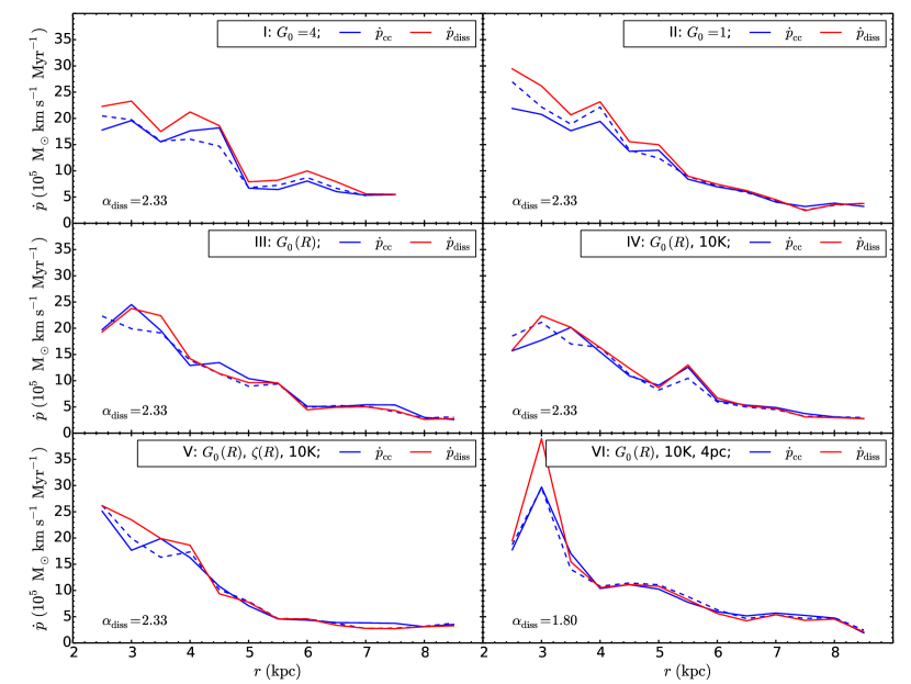
In Figure 24 we show the radial profiles of $\dot{p}_{\rm CC}$ in the simulations, evaluated from 200 to 300 Myr and averaged over all GMCs. As expected from our previous results, the momentum injection rate per GMC is highest in the inner galaxy. It is then seen to decline by about a factor of $\sim 5$ as one progresses outwards to $\sim 8\>$kpc.

The rate of dissipation of the total internal turbulent momentum, $p_{c}$, of a GMC can be expressed as (Tan et al., 2013):

$$\dot{p}_{\rm diss} \equiv -p_{c}/(\alpha_{\rm diss}t_{\rm ff})=-\sqrt{3}\bar{M}_{c}\sigma_{c}/(\alpha_{\rm diss}t_{\rm ff})$$ (17)

$$= -2.19\bar{\alpha}_{\rm vir}^{1/2}G\bar{M}_{c}\bar{\Sigma}_{c}/\alpha_{\rm diss},$$

where $\alpha_{\rm diss}$ is a dimensionless constant. The turbulent energy dissipation rate has been measured in numerical simulations to be $\epsilon_{\rm diss}=(1/2)(\dot{E}/{E})[l_{0}/(\sqrt{3}\sigma)]\simeq 0.6$ (see review by McKee & Ostriker (2007)), so that $\alpha_{\rm diss}\simeq 3.85$ (in a cloud with $\alpha_{\rm vir}\simeq 1$ and $l_{0}=2R$). Figure 24 also shows the radial profiles of $\dot{p}_{\rm diss}$, but where we have allowed $\alpha_{\rm diss}$ to vary (fixing a single value for Runs I to V, and another value for the higher resolution Run VI) to obtain a close match between $\dot{p}_{\rm diss}$ and $\dot{p}_{\rm CC}$. This requires values of $\alpha_{\rm diss}\simeq 2$, i.e., a shorter dissipation timescale that is about half the theoretical expectation of $\simeq 4t_{\rm ff}$, which is not unexpected given the fact the GMCs in our simulations are only quite poorly resolved. Alternatively, agreement could be achieved at lower values of $\dot{p}$ by reducing the efficiency of conversion of the bulk collision momentum to internal turbulent momentum to about 50% in equation (16). However, the most important point of Figure 24 is that the radial profiles of $\dot{p}_{\rm diss}$ and $\dot{p}_{\rm CC}$ are very similar, suggesting there is a physical link between them.

Finally, we balance the momentum injection rate due to cloud collisions, given by eq. (16), with the dissipation rate within the clouds, given by eq. (17), to predict typical GMC equilibrium mass surface densities, $\bar{\Sigma}_{c,{\rm eq}}$.

$$\bar{\Sigma}_{c,{\rm eq}} = 102\bar{\alpha}_{\rm vir}^{-1/2}\frac{\alpha_{\rm diss}}{2}\frac{b^{\prime}}{1.6}\frac{0.2}{f_{\rm coll}}\left(\frac{\bar{M}_{c}}{10^{6}\>M_{\odot}}\right)^{1/3}$$ (18)

$$\times \left(\frac{v_{\rm circ}}{200\>{\rm km\>s^{-1}}}\frac{4\>{\rm kpc}}{r}\right)^{4/3}M_{\odot}\>{\rm pc^{-2}}.$$

Figure 25 shows the predicted radial dependence of $\bar{\Sigma}_{c,{\rm eq}}$ from eq. (18), which is calculated by assessing the values of $\bar{M}_{c}$, $\bar{\alpha}_{\rm vir}$ and $\bar{f}_{\rm coll}$ in each annulus. The figure also compares these estimates with the actual values of the mass surface densities of the GMCs in the simulations. Since the values of $\alpha_{\rm diss}$ have been normalized so that $\dot{p}_{\rm diss}\simeq\dot{p}_{\rm CC}$, we expect that $\bar{\Sigma}_{c,{\rm eq}}$ will on average be approximately equal to $\bar{\Sigma}_{c}$, as is seen to be the case. Still, the close correspondence of the radial profiles of $\bar{\Sigma}_{c,{\rm eq}}$ and $\bar{\Sigma}_{c}$, i.e., for a single value of $\alpha_{\rm diss}$, indicates that the average structural properties of these self-gravitating GMCs are being set by the injection of turbulent momentum from GMC collisions, balanced by its rate of decay at a rate inversely proportional to the local free-fall time.

The equilibrium condition described by eq. (18) is expected to be prone to instability, since as GMCs become denser and smaller, they dissipate their turbulent momentum at a faster absolute rate given their shorter free-fall times. At the same time, being smaller, they are expected to be less likely to under collisions. In reality, the processes of $B$-field support, star formation and feedback are expected to also play a role in regulating the structure of these densest, collapsing GMCs. In the current simulations, lacking these processes, we expect that numerical diffusion and viscosity due to the fast, supersonic motion of the GMCs in their orbits in the galactic potential leads to some effective support of GMCs that become too small. In this way, a quasi-equilibrium distribution of GMC properties can still be established in these simulations (see also TT09).

Figure 25: Predicted mean GMC mass surface densities, $\bar{\Sigma}_{\rm eq}$ (red solid lines), measured from 200 to 300 Myr and shown as a function of galactocentric radius for Runs I to VI (panels as labelled). This estimate is based on a model of a balance between the momentum injection rate by GMC-GMC collisions and the internal dissipation rate resulting from supersonic turbulence, parameterized by $\alpha_{\rm diss}$ (see text). The actual mean GMC mass surface densities, $\bar{\Sigma}_{c}$ (blue solid lines), are also shown. The similarity of the radial profiles of $\Sigma$ of the GMCs indicates that their structure can be explained by a simple model in which their internal turbulence is driven by GMC collisions and decays at a rate that is inversely proportional to the local free-fall time.

5.5 General Implications of Short GMC Collision Timescales

Short GMC collision timescales have several important implications. First, we have already seen in §5.4 that frequent GMC collisions could be an important driver of turbulence within the clouds. This mechanism could then regulate the structure of GMCs, i.e., setting their mass surface densities. The relative importance of GMC collisions and star formation feedback at driving internal turbulence needs to be assessed by future studies.

Second, GMC collisions may set the angular momentum distribution of the clouds, in particular helping to explain the relatively high fraction of retrograde rotation directions (Koda & Sofue, 2006; Imara & Blitz, 2011; Imara et al., 2011) (see also Fig. 18f and 19f).

Third, if $t_{\rm coll}$ is $\lesssim 30\>$Myr, then the collision time is shorter or similar to estimates of GMC lifetimes due to feedback (Williams & McKee, 1997; Matzner, 2002; Krumholz et al., 2006). This changes the nature of the life cycle of GMCs, since they are continually changing and replenishing their gas content by collisions with other GMCs at rates similar to those at which they are losing gas by energy and momentum injection from massive stars. Thus the “lifetime” of GMCs no longer has its traditional meaning, i.e., the time before the GMC is dispersed to theq atomic or ionized phase of the ISM, since the clock is essentially “reset” after every major collision.

Fourth, GMC collisions may induce star formation, i.e., by compressing gas that is already on the verge of gravitational instability in the pre-collision GMCs. The compressed region, with enhanced turbulence and large velocity gradients, may have its rates of ambipolar diffusion (e.g., Mouschovias (1991); Kunz & Mouschovias (2009)) and/or reconnection diffusion (Lazarian & Vishniac, 1999; Eyink et al., 2011) boosted, thus helping remove magnetic flux and triggering gravitational instabilty and then star cluster formation. Shear-driven GMC collisions is a process that naturally connects the kiloparsec scales of galactic orbital dynamics to the parsec scales of star cluster formation. There have been numerous claims of GMC collisions being the triggering agents of star cluster formation: e.g., Westerlund 2 (Furukawa et al., 2009; Ohama et al., 2010), M20 (Torii et al., 2011), Cygnus OB 7 (Dobashi et al., 2014), and N159 West (Fukui et al., 2015). GMC collisions are also a natural mechanism for creating the large observed dispersion in the star formation efficiencies in GMCs (e.g., Tan (2000); Lee et al. (2016)).

6 Conclusions

We have simulated flat rotation curve galactic gas disks and investigated the dynamical evolution of their interstellar media and GMCs. Based on PDR models, we incorporated a self-consistent treatment of the ISM physics of the atomic to molecular phase transition under the influence of various background FUV radiation fields and CR ionization rates. We then explored the effects of different FUV intensities, including a model with a radial gradient designed to mimic the Milky Way galaxy. The effects of cosmic rays, including radial gradients in their heating and ionization rates, were also investigated. The final simulation in this series achieved 4 pc resolution across the $\sim 20$ kpc global disk diameter, with heating and cooling followed down to $\sim 10$ K temperatures. The galaxies were evolved for 300 Myr, i.e., long enough for ISM and GMC properties to achieve a quasi steady state. We found that during the period of simulations, the initially marginally stable ISM fragmented into GMCs due to radiative cooling and gravitational instability. GMC properties then became influenced by frequent interactions, including collisions.

We examined global ISM properties, including the mass surface density structures, thermal pressures, and the evolution and spatial distribution of GMC mass fractions, as well as the GMC mass traced by CO with $n_{\rm CO}/n_{\mathrm{H}}>10^{-5}{\rm cm^{-3}}$. Our results show that strong FUV fields can suppress global GMC formation, especially in the outer regions where gas is more diffuse. Our fiducial model has a radial profile of molecular mass fraction that is quite similar to that observed in the Milky Way out to $\sim 6\>$kpc by Koda et al. (2016). The lack of the additional physics of localized star formation feedback is likely the main cause of the higher molecular fractions seen in our simulations at larger radii.

We also analyzed GMC properties, including distribution functions of mass, mass surface density, effective radii, vertical locations, virial parameters and specific angular momenta. Though we only incorporated diffuse FUV heating and CR ionization, many observed GMC properties are approximately reproduced, including the mass spectrum, mass surface density distribution, and angular momentum distribution, which shows that retrograde clouds are relatively common. The distribution of virial parameters shows a large fraction of gravitationally bound clouds, along with a population of super-virial clouds potentially caused by strong and frequent cloud-cloud interactions. We notice that these GMC properties are relatively insensitive to our different implementations of diffuse FUV and CR heating, implying rather the important role of GMC interactions.

Finally GMC collisions, which may be a means of triggering star cluster formation, were investigated and compared with analytic models of galactic shear-induced collisions. Our results show an approximate agreement with the models, and insensitivity to parameters related to the diffuse heating. The average collision timescale is relatively short, i.e., $\sim 0.1$ to 0.2 times the local orbital time. Such frequent GMC collisions may be an important driver of turbulence in the clouds, potentially explaining their observed structural, kinematic and dynamical properties.

The simulations so far presented lack several important pieces of physics, especially magnetic fields and localized star formation feedback. These aspects, along with the effects of different galactic dynamical environments, including spiral arms, will be studied in future papers in this series.

Computations described in this work were performed using the publicly available Enzo code (http://enzo-project.org). This research also made use of the yt-project (http://yt-project. org/), a toolkit for analyzing and visualizing quantitative data Turk et al. (2011). These are products of collaborative efforts of many independent scientists from numerous institutions around the world. Their commitment to open science has helped make this work possible. The authors acknowledge University of Florida Research Computing (www.rc.ufl.edu) for providing computational resources and support that have contributed to the research results reported in this publication.

References

- Agertz et al. (2013) Agertz, O., Kravtsov, A. V., Leitner, S. N., & Gnedin, N. Y. 2013, ApJ, 770, 25
- Agertz & Kravtsov (2015) Agertz, O., & Kravtsov, A. V. 2015, ApJ, 804, 18
- Bertoldi & McKee (1992) Bertoldi, F., & McKee, C. F. 1992, ApJ, 395, 140
- Bialy & Sternberg (2015) Bialy, S., & Sternberg, A. 2015, MNRAS, 450, 4424
- Bigiel et al. (2008) Bigiel, F., Leroy, A., Walter, F., et al. 2008, AJ, 136, 2846
- Bihr et al. (2015) Bihr, S., Beuther, H., Ott, J., et al. 2015, A&A, 580, A112
- Binney & Tremaine (1987) Binney, J., & Tremaine, S. 1987, Princeton, NJ, Princeton University Press, 1987, 747 p.
- Bisbas et al. (2015) Bisbas, T. G., Papadopoulos, P. P., & Viti, S. 2015, ApJ, 803, 37
- Bisbas et al. (2017) Bisbas, T. G., van Dishoeck, E. F., Papadopoulos, P. P., et al. 2017, ApJ, 839, 90
- Blitz (1990) Blitz, L. 1990, The Evolution of the Interstellar Medium, 12, 273
- Blitz (1993) Blitz, L. 1993, Protostars and Planets III, 125
- Boulares & Cox (1990) Boulares, A., & Cox, D. P. 1990, ApJ, 365, 544
- Bryan et al. (2014) Bryan, G. L., Norman, M. L., O’Shea, B. W., et al. 2014, ApJS, 211, 19
- Butler et al. (2015) Butler, M. J., Tan, J. C., & Van Loo, S. 2015, ApJ, 805, 1
- Butler et al. (2017) Butler, M. J., Tan, J. C., Teyssier, R., et al. 2017, arXiv:1703.04509
- Daddi et al. (2010) Daddi, E., Elbaz, D., Walter, F., et al. 2010, ApJ, 714, L118
- Dalgarno (2006) Dalgarno, A. 2006, Proceedings of the National Academy of Science, 103, 12269
- Dobashi et al. (2014) Dobashi, K., Matsumoto, T., Shimoikura, T., et al. 2014, ApJ, 797, 58
- Dobbs (2008) Dobbs, C. L. 2008, MNRAS, 391, 844
- Dobbs et al. (2017) Dobbs, C. L., Adamo, A., Few, C. G., et al. 2017, MNRAS, 464, 3580
- Dobbs et al. (2011) Dobbs, C. L., Burkert, A., & Pringle, J. E. 2011, MNRAS, 417, 1318
- Dobbs & Pringle (2013) Dobbs, C. L., & Pringle, J. E. 2013, MNRAS, 432, 653
- Draine (1978) Draine, B. T. 1978, ApJS, 36, 595
- Eyink et al. (2011) Eyink, G. L., Lazarian, A., & Vishniac, E. T. 2011, ApJ, 743, 51
- Ferland et al. (2013) Ferland, G. J., Porter, R. L., van Hoof, P. A. M., et al. 2013, RMxAA, 49, 137
- Fujimoto et al. (2014) Fujimoto, Y., Tasker, E. J., Wakayama, M., & Habe, A. 2014, MNRAS, 439, 936
- Fujimoto et al. (2016) Fujimoto, Y., Bryan, G. L., Tasker, E. J., Habe, A., & Simpson, C. M. 2016, MNRAS, 461, 1684
- Fukui et al. (2015) Fukui, Y., Harada, R., Tokuda, K., et al. 2015, ApJ, 807, L4
- Furukawa et al. (2009) Furukawa, N., Dawson, J. R., Ohama, A., et al. 2009, ApJ, 696, L115
- Gammie et al. (1991) Gammie, C. F., Ostriker, J. P., & Jog, C. J. 1991, ApJ, 378, 565
- Genzel et al. (2010) Genzel, R., Tacconi, L. J., Gracia-Carpio, J., et al. 2010, MNRAS, 407, 2091
- Goldbaum et al. (2011) Goldbaum, N. J., Krumholz, M. R., Matzner, C. D., & McKee, C. F. 2011, ApJ, 738, 101
- Goldbaum et al. (2015) Goldbaum, N. J., Krumholz, M. R., & Forbes, J. C. 2015, ApJ, 814, 131
- Goldbaum et al. (2016) Goldbaum, N. J., Krumholz, M. R., & Forbes, J. C. 2016, ApJ, 827, 28
- Gratier et al. (2012) Gratier, P., Braine, J., Rodriguez-Fernandez, N. J., et al. 2012, A&A, 542, A108
- Habing (1968) Habing, H. J. 1968, Bull. Astron. Inst. Netherlands, 19, 421
- Heitsch et al. (2005) Heitsch, F., Burkert, A., Hartmann, L. W., Slyz, A. D., & Devriendt, J. E. G. 2005, ApJ, 633, L113
- Heyer et al. (2009) Heyer, M., Krawczyk, C., Duval, J., & Jackson, J. M. 2009, ApJ, 699, 1092
- Hopkins et al. (2013) Hopkins, P. F., Narayanan, D., Murray, N., & Quataert, E. 2013, MNRAS, 433, 69
- Hopkins et al. (2014) Hopkins, P. F., Kereš, D., Oñorbe, J., et al. 2014, MNRAS, 445, 581
- Hopkins et al. (2011) Hopkins, P. F., Quataert, E., & Murray, N. 2011, MNRAS, 417, 950
- Hopkins et al. (2012) Hopkins, P. F., Quataert, E., & Murray, N. 2012, MNRAS, 421, 3488
- Imara & Blitz (2011) Imara, N., & Blitz, L. 2011, ApJ, 732, 78
- Imara et al. (2011) Imara, N., Bigiel, F., & Blitz, L. 2011, ApJ, 732, 79
- Inoue & Inutsuka (2008) Inoue, T., & Inutsuka, S.-i. 2008, ApJ, 687, 303-310
- Inoue & Inutsuka (2012) Inoue, T., & Inutsuka, S.-i. 2012, ApJ, 759, 35
- Kainulainen et al. (2009) Kainulainen, J., Beuther, H., Henning, T., & Plume, R. 2009, A&A, 508, L35
- Kennicutt (1998) Kennicutt, R. C., Jr. 1998, ApJ, 498, 541
- Kennicutt & Evans (2012) Kennicutt, R. C., & Evans, N. J. 2012, ARA&A, 50, 531
- Kim et al. (2003) Kim, W.-T., Ostriker, E. C., & Stone, J. M. 2003, ApJ, 599, 1157
- Koda et al. (2016) Koda, J., Scoville, N., & Heyer, M. 2016, ApJ, 823, 76
- Koda & Sofue (2006) Koda, J., & Sofue, Y. 2006, PASJ, 58, 299
- König et al. (2016) König, S., Martín, S., Muller, S., et al. 2016, arXiv:1612.07668
- Körtgen & Banerjee (2015) Körtgen, B., & Banerjee, R. 2015, MNRAS, 451, 3340
- Krumholz et al. (2006) Krumholz, M. R., Matzner, C. D., & McKee, C. F. 2006, ApJ, 653, 361
- Krumholz & McKee (2005) Krumholz, M. R., & McKee, C. F. 2005, ApJ, 630, 250
- Krumholz & Tan (2007) Krumholz, M. R., & Tan, J. C. 2007, ApJ, 654, 304
- Kunz & Mouschovias (2009) Kunz, M. W., & Mouschovias, T. C. 2009, MNRAS, 399, L94
- Lazarian & Vishniac (1999) Lazarian, A., & Vishniac, E. T. 1999, ApJ, 517, 700
- Lee et al. (2016) Lee, E. J., Miville-Deschênes, M.-A., & Murray, N. W. 2016, ApJ, 833, 229
- Leroy et al. (2008) Leroy, A. K., Walter, F., Brinks, E., et al. 2008, AJ, 136, 2782
- Leroy et al. (2013) Leroy, A. K., Walter, F., Sandstrom, K., et al. 2013, AJ, 146, 19
- Mac Low et al. (1998) Mac Low, M.-M., Klessen, R. S., Burkert, A., & Smith, M. D. 1998, Physical Review Letters, 80, 2754
- Matzner (2002) Matzner, C. D. 2002, ApJ, 566, 302
- Mayer et al. (2016) Mayer, L., Tamburello, V., Lupi, A., et al. 2016, ApJ, 830, L13
- McKee & Ostriker (2007) McKee, C. F., & Ostriker, E. C. 2007, ARA&A, 45, 565
- Miville-Deschênes et al. (2017) Miville-Deschênes, M.-A., Murray, N., & Lee, E. J. 2017, ApJ, 834, 57
- Momose et al. (2010) Momose, R., Okumura, S. K., Koda, J., & Sawada, T. 2010, ApJ, 721, 383
- Mouschovias (1991) Mouschovias, T. C. 1991, ApJ, 373, 169
- Ohama et al. (2010) Ohama, A., Dawson, J. R., Furukawa, N., et al. 2010, ApJ, 709, 975
- Oka et al. (2001) Oka, T., Hasegawa, T., Sato, F., et al. 2001, ApJ, 562, 348
- Padoan & Nordlund (2002) Padoan, P., & Nordlund, Å. 2002, ApJ, 576, 870
- Phillips (1999) Phillips, J. P. 1999, A&AS, 134, 241
- Read et al. (2016) Read, J. I., Agertz, O., & Collins, M. L. M. 2016, MNRAS, 459, 2573
- Rosolowsky et al. (2003) Rosolowsky, E., Engargiola, G., Plambeck, R., & Blitz, L. 2003, ApJ, 599, 258
- Roman-Duval et al. (2010) Roman-Duval, J., Jackson, J. M., Heyer, M., Rathborne, J., & Simon, R. 2010, ApJ, 723, 492
- Röllig et al. (2007) Röllig, M., Abel, N. P., Bell, T., et al. 2007, A&A, 467, 187
- Safranek-Shrader et al. (2017) Safranek-Shrader, C., Krumholz, M. R., Kim, C.-G., et al. 2017, MNRAS, 465, 885
- Sheth et al. (2002) Sheth, K., Vogel, S. N., Regan, M. W., et al. 2002, AJ, 124, 2581
- Smith et al. (2017) Smith, B. D., Bryan, G. L., Glover, S. C. O., et al. 2017, MNRAS, 466, 2217
- Sobolev (1957) Sobolev, V. V. 1957, Soviet Ast., 1, 678
- Solomon et al. (1987) Solomon, P. M., Rivolo, A. R., Barrett, J., & Yahil, A. 1987, ApJ, 319, 730
- Stone & Norman (1992) Stone, J. M., & Norman, M. L. 1992, ApJS, 80, 753
- Stone et al. (1998) Stone, J. M., Ostriker, E. C., & Gammie, C. F. 1998, ApJ, 508, L99
- Suwannajak et al. (2014) Suwannajak, C., Tan, J. C., & Leroy, A. K. 2014, ApJ, 787, 68
- Tan (2000) Tan, J. C. 2000, ApJ, 536, 173
- Tan (2010) Tan, J. C. 2010, ApJ, 710, L88
- Tan et al. (2013) Tan, J. C., Shaske, S. N., & Van Loo, S. 2013, Molecular Gas, Dust, and Star Formation in Galaxies, 292, 19
- Tasker (2011) Tasker, E. J. 2011, ApJ, 730, 11
- Tasker & Tan (2009) Tasker, E. J., & Tan, J. C. 2009, ApJ, 700, 358
- Tasker et al. (2015) Tasker, E. J., Wadsley, J., & Pudritz, R. 2015, ApJ, 801, 33
- Truelove et al. (1997) Truelove, J. K., Klein, R. I., McKee, C. F., et al. 1997, ApJ, 489, L179
- Toomre (1964) Toomre, A. 1964, ApJ, 139, 1217
- Torii et al. (2011) Torii, K., Enokiya, R., Sano, H., et al. 2011, ApJ, 738, 46
- Turk et al. (2011) Turk, M. J., Smith, B. D., Oishi, J. S., et al. 2011, ApJS, 192, 9
- von Neumann & Richtmyer (1950) von Neumann, J., & Richtmyer, R. D. 1950, Journal of Applied Physics, 21, 232
- Van Loo et al. (2013) Van Loo, S., Butler, M. J., & Tan, J. C. 2013, ApJ, 764, 36
- Van Loo et al. (2015) Van Loo, S., Tan, J. C., & Falle, S. A. E. G. 2015, ApJ, 800, L11
- Vázquez-Semadeni et al. (2011) Vázquez-Semadeni, E., Banerjee, R., Gómez, G. C., et al. 2011, MNRAS, 414, 2511
- Wannier et al. (1991) Wannier, P. G., Lichten, S. M., Andersson, B.-G., & Morris, M. 1991, ApJS, 75, 987
- Williams & McKee (1997) Williams, J. P., & McKee, C. F. 1997, ApJ, 476, 166
- Wolfire et al. (2003) Wolfire, M. G., McKee, C. F., Hollenbach, D., & Tielens, A. G. G. M. 2003, ApJ, 587, 278
- Wolfire et al. (2010) Wolfire, M. G., Hollenbach, D., & McKee, C. F. 2010, ApJ, 716, 1191
- Wu et al. (2017a) Wu, B., Tan, J. C., Nakamura, F., et al. 2017, ApJ, 835, 137
- Wu et al. (2017b) Wu, B., Tan, J. C., Christie, D., et al. 2017, ApJ, 841, 88
- Wu et al. (2015) Wu, B., Van Loo, S., Tan, J. C., & Bruderer, S. 2015, ApJ, 811, 56
- Zuckerman & Evans (1974) Zuckerman, B., & Evans, N. J., II 1974, ApJ, 192, L14