- CT
- computed tomography
- HNN
- holistically-nested network
- P-HNN
- progressive holistically-nested network
- ILD
- interstitial lung disease
- LTRC
- Lung Tissue Research Consortium
- CNN
- convolutional neural network
- FCN
- fully convolutional network
- PLS
- pathological lung segmentation
- DS
- Dice score
- CNN
- convolutional neural network
- ASD
- average surface distance
- COPD
- chronic obstructive pulmonary disease
- CV
- cross-validation
- NIH
- National Institutes of Health
- UHG
- University Hospitals of Geneva
- ILD
- interstitial lung disease
- HU
- Hounsfield unit
Progressive and Multi-Path Holistically Nested Neural Networks for Pathological Lung Segmentation from CT Images
Abstract
Pathological lung segmentation (PLS) is an important, yet challenging, medical image application due to the wide variability of pathological lung appearance and shape. Because PLS is often a pre-requisite for other imaging analytics, methodological simplicity and generality are key factors in usability. Along those lines, we present a bottom-up deep-learning based approach that is expressive enough to handle variations in appearance, while remaining unaffected by any variations in shape. We incorporate the deeply supervised learning framework, but enhance it with a simple, yet effective, progressive multi-path scheme, which more reliably merges outputs from different network stages. The result is a deep model able to produce finer detailed masks, which we call progressive holistically-nested networks (P-HNNs). Using extensive cross-validation, our method is tested on multi-institutional datasets comprising CT scans ( publicly available), of pathological lungs, reporting mean dice scores of and demonstrating significant qualitative and quantitative improvements over state-of-the art approaches.
Keywords:
progressive and multi-path convolutional neural networks, holistically nested neural networks, pathological lung segmentation
1 Introduction
Pulmonary diseases are a major source of death and hospitalization worldwide, with computed tomography (CT) a leading modality for screening [9]. Thus, there is great impetus to develop tools for automated detection and diagnosis from CT. Reliable pathological lung segmentation (PLS) is a cornerstone of this goal, ensuring that disease detection is not confounded by regions outside the lung [9, 3]. Moreover, PLS is also innately useful, e.g., measuring lung volume. To be effective, PLS must handle the wide variability in appearance that abnormalities can cause.
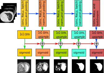
Leading PLS approaches often rely on prior 3D shape or anatomical landmark localization [9, 4, 15]. This top-down approach can help delineate regions hard to discriminate based on intensity features alone. However, all shape or localization variations must be accounted for [3, 9]. For instance, the image acting as input in Fig. 1, which is of a patient with only one lung, could severely challenge a top-down method that fails to account for this variation.
In contrast, with effective image features, a bottom-up approach, i.e., one that classifies individual pixels or patches, would, in principle, be able to handle most cases with challenging shapes seamlessly. Existing fully bottom-up PLS methods [16, 5] show promise, but the authors of both state their methods can struggle with severe pathologies. Instead, a fruitful direction for PLS is deep fully convolutional networks, which currently represents the state-of-the-art within computer vision [8, 7] and medical imaging analysis [13, 12, 11, 1, 10] for segmentation.
Motivated by these developments, we apply a bottom-up FCN approach to PLS. Given that PLS is often a first step prior to subsequent analysis, we place a high premium on simplicity and robustness. For this reason, our approach adapts the highly effective, yet straightforward, holistically-nested network (HNN) deep-learning architecture [17]. To overcome issues with HNN output ambiguity and the well-known coarsening resolution of FCNs, we introduce a simple, but surprisingly powerful, multi-path enhancement. Unlike other multi-path works [7, 1, 10], that use complex coarse-to-fine pathways, we opt for a progressive constraint on multi-scale pathways that requires no additional convolutional layers or network parameters. The result is an effective and uncomplicated PLS solution that we call progressive holistically-nested networks.
Focusing on infection-, interstitial lung disease (ILD)-, and chronic obstructive pulmonary disease (COPD)-based pathologies, we test our method on a multi-institute dataset consisting of challenging thoracic CT scans exhibiting a variety of pathology patterns, including consolidations, infiltrations, fibroses, pleural effusions, lung cavities, and emphysema. This is the largest analysis to date for assessing PLS performance. Importantly, of the CT scans are publicly available, allowing future methods to directly compare performance. We report quantitative five-fold cross-validated metrics, providing a more realistic picture of our tool’s generalizability than prior work [9, 4, 5, 15, 16]. With this dataset, we obtain average Dice-scores of . We share our tool online for researchers’ use and testing111https://adampharrison.gitlab.io/p-hnn/.
2 Methods

We will first focus on aspects shared with HNNs and then discuss the progressive multi-path enhancement of P-HNNs.
To begin, we denote the training data as , where and represent the input and binary ground-truth images, respectively. The HNN model, originally called holistically-nested edge detection [17], is a type of FCN [8], meaning layer types are limited to convolutional, pooling, and nonlinear activations. HNNs are built off of a standard convolutional neural network (CNN), e.g., the VGG-16 model [14], that runs each image through stages, separated by pooling layers. Unlike the original HNN, we use batch normalization after each stage. We denote all network parameters of these standard layers as .
HNNs popularized the concept of deep supervision to FCNs, which is based on the intuition that deeper layers have access to both higher levels of abstraction but coarser levels of scale. As depicted in the green arrows of Fig. 1, the novelty of HNNs is the use of deep supervision to guide the training by computing side-outputs, and their loss, at intermediate stages. HNNs also merge predictions from different network stages, allowing different levels and scales to contribute to the final result.
More formally, a set of convolutional weights collapses the last activation maps of each stage into an image, i.e., for stage , sample , and pixel location . After upsampling to the original resolution, masks at intermediate stages are estimated using
| (1) | ||||
| (2) | ||||
| (3) |
where denotes the sigmoid function and and represent the pixel- and image-level estimates, respectively. We drop for the remainder of this explanation.
The cross-entropy loss at each side-output can then be calculated using
| (4) |
where represents a constant and global class-balancing weight, which we observe provides better PLS results than Xie et al.’s [17] original image-specific class-balancing scheme. We also prefer to use a sample estimate of the population balance, since we train on an entire training set, and not just on individual images. Not shown in Fig. 1, HNNs also output a final fused probability map based on a learned weighted sum of .
While highly effective, HNNs suffer from two issues. The first is inconsistency of the fused output, where certain side outputs on their own can sometimes provide superior results than the final fused output. This is reflected by Xie et al.’s use of different outputs depending on the dataset [17]. Ideally, there should be an obvious, and optimal, output to use.
The second issue is one shared by many early FCN solutions—that while deeper stages have greater levels of abstraction, their activations are also coarser in spatial resolution, hampering the capture of fine-level details. This issue is often addressed using multi-path connections [7, 1, 10] that typically use complex coarse-to-fine pathways to combine activations from earlier stages with later ones, e.g., the ubiquitous “U”-like structure [7, 1, 10]. Multiple convolutional layers [1, 10] or even sub-networks [7] are used to combine activations. Of these, only Merkow et al. incorporate both multi-path connections and deep supervision [10], but their solution relies on a three-stage training process, in addition to the extra coarse-to-fine pathway.
While these solutions are effective, they require additional parameters totalling nearly the same number as [1, 10], or more than [7], the original FCN path. Following our philosophy of favoring simplicity, we instead propose a more straightforward progressive multi-path connection. As illustrated in Fig. 1, we combine activations from the current and previous stages using simple addition prior to applying the sigmoid function. Formally, our model alters the HNN formulation by modifying (3) to
| (5) |
As activations can exhibit negative or positive values, (5) forces side outputs to improve upon previous outputs, by adding to or subtracting from the corresponding activation. For this reason, we call the model progressive holistically-nested networks (P-HNNs). This progressive enhancement allows P-HNNs to jettison the fused output, avoiding the inconsistent output of HNNs. Like other multi-path solutions, gradient backpropagation cascades through multiple connections. Unlike other solutions, this enhanced new capability is realized with minimal complexity, requiring fewer parameters than standard HNNs.
Implementation Details: We train and test our method on 2D axial CT slices, using three windows of , , and Hounsfield units to rescale each slice to a -channel -bit image. While 3D FCNs have been reported [1, 10], these rely on numerous sliding boxes, each with a limited field-of-view. Because lung regions occupy significant portions of a CT scan, large spatial contexts may be needed for accurate segmentation. In addition, due to memory and computational constraints, 3D CNNs are often less deep and wide than 2D variants. Moreover, recent work has demonstrated that 2D CT slices are expressive enough for segmenting complex organs [12, 13, 18]. Finally, inter-slice thicknesses of low-dose screening CTs can range from to . The associated spatial discontinuities could severely challenge 3D-based methods. In contrast, 2D P-HNNs can work well for any inter-slice thickness. Thus, we opt for a 2D approach, which remains simple and requires no reduction in CNN field-of-view, depth, and width.
3 Experiments
| (a) | (b) | (c) | (d) | (e) |
| (a) | (b) | (c) | (d) | (e) |
We measure PLS performance using multi-institutional data from the Lung Tissue Research Consortium (LTRC) ILD/COPD dataset [6], the University Hospitals of Geneva (UHG) ILD dataset [2], and a subset of an infection-based dataset from the National Institutes of Health (NIH) Clinical Center [9]222Due to a data-archiving issue, Mansoor et al. were only able to share 88 CT scans, and, of those, only 47 PLS masks produced by their method [9].. LTRC masks were initially generated using an automatic method, followed by visual inspection and manual correction if necessary [6]. For all datasets, we also visually inspect and exclude scan/mask pairs with annotation errors. This results in , , and CT scans from the LTRC, UHG and NIH datasets, respectively.
Using five-fold cross-validation (CV), separated at the patient and dataset level, we train on every tenth slice of the LTRC dataset and all slices of the other two. We fine-tuned from an ImageNet pre-trained VGG-16 model [14], halting training after roughly epochs. Validation subsets determined probability-map thresholds. Post-processing simply fills any 3D holes and keeps the largest two connected components if the volume ratio between the two is less than , otherwise only the largest is kept. Depending on the number of slices, our system takes roughly to segment one volume using a Tesla K40.
Table 1(a) depicts
| Dataset Model DS ASD (mm) LTRC HNN P-HNN UHG HNN P-HNN NIH HNN P-HNN Total HNN P-HNN | Model DS ASD (mm) Mansoor et al. [9] P-HNN |
| (a) | (b) |
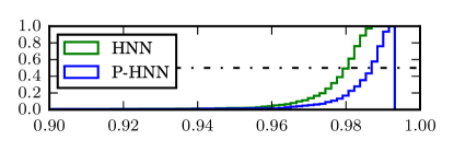
the mean 3D Dice scores and average surface distances of HNN versus P-HNN. As can be seen, while HNN posts very good DSs and ASDs of and mm, respectively, P-HNN is able to outperform it, posting even better values ( Wilcox signed-rank test) of and mm, respectively. Fig. 4(a) depicts cumulative DS histograms, visually illustrating the distribution of improvements in segmentation performance. Fig. 2 depicts selected qualitative examples, demonstrating the effect of these quantitative improvements in PLS-mask visual quality and usefulness.
 |
 |
| (a) | (b) |
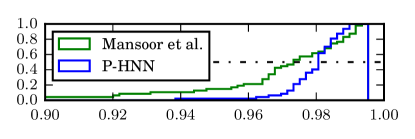
Using volumes from the NIH dataset, we also test against Mansoor et al.’s non deep-learning method [9], which produced state-of-the-art performance on challenging and varied infectious disease CT scans. As Table 1(b) and Fig. 4(b) illustrate, P-HNN significantly () outperforms this previous state-of-the-art approach, producing much higher DSs. ASD scores were also better, but statistical significance was not achieved for this metric. Lastly, as shown in Fig. 3, P-HNN generates PLS masks with considerable qualitative improvements.
4 Conclusion
This work introduced P-HNNs, an FCN-based [8] deep-learning tool for PLS that combines the powerful concepts of deep supervision and multi-path connections. We address the well-known FCN coarsening resolution problem using a progressive multi-path enhancement, which, unlike other approaches [7, 1, 10], requires no extra parameters over the base FCN. When tested on thoracic CT scans exhibiting infection-, ILD-, and COPD-based pathologies, the largest evaluation of PLS to-date, P-HNN consistently outperforms () standard HNN, producing mean DSs of . P-HNN also provides significantly improved PLS masks compared against a state-of-the-art tool [9]. Thus, P-HNNs offer a simple, yet highly effective, means to produce robust PLS masks. The P-HNN model can also be applied to pathological lungs with other morbidities and could provide a straightforward and powerful tool for other segmentation tasks.
References
- [1] Çiçek, Ö., Abdulkadir, A., Lienkamp, S.S., Brox, T., Ronneberger, O.: 3d u-net: Learning dense volumetric segmentation from sparse annotation. In: MICCAI 2016, Proceedings, Part II. pp. 424–432 (2016)
- [2] Depeursinge, A., Vargas, A., Platon, A., Geissbuhler, A., Poletti, P.A., Müller, H.: Building a reference multimedia database for interstitial lung diseases. Computerized Medical Imaging and Graphics 36(3), 227–238 (2012)
- [3] El-Baz, A., Beache, G.M., Gimel’farb, G.L., Suzuki, K., Okada, K., Elnakib, A., Soliman, A., Abdollahi, B.: Computer-aided diagnosis systems for lung cancer: Challenges and methodologies. Int. J. Biomedical Imaging (2013)
- [4] Gill, G., Beichel, R.: Segmentation of lungs with interstitial lung disease in ct scans: A tv-l1 based texture analysis approach. ISVC pp. 511–520 (2014)
- [5] Hosseini-Asl, E., Zurada, J.M., Gimel’farb, G., El-Baz, A.: 3-d lung segmentation by incremental constrained nonnegative matrix factorization. IEEE Trans. on Biomedical Engineering 63(5), 952–963 (2016)
- [6] Karwoski, R.A., Bartholmai, B., Zavaletta, V.A., Holmes, D., Robb, R.A.: Processing of ct images for analysis of diffuse lung disease in the lung tissue research consortium. In: Proc. SPIE 6916, Medical Imaging 2008: Physiology, Function, and Structure from Medical Images (2008)
- [7] Lin, G., Milan, A., Shen, C., Reid, I.: RefineNet: Multi-path refinement networks for high-resolution semantic segmentation. arXiv:1611.06612 (Nov 2016)
- [8] Long, J., Shelhamer, E., Darrell, T.: Fully convolutional networks for semantic segmentation. In: IEEE CVPR. pp. 3431–3440 (2015)
- [9] Mansoor, A., Bagci, U., Xu, Z., Foster, B., Olivier, K.N., Elinoff, J.M., Suffredini, A.F., Udupa, J.K., Mollura, D.J.: A generic approach to pathological lung segmentation. IEEE Trans. on Medical Imaging 33(12), 2293–2310 (2014)
- [10] Merkow, J., Marsden, A., Kriegman, D.J., Tu, Z.: Dense volume-to-volume vascular boundary detection. In: MICCAI 2016, Proceedings, Part III. pp. 371–379 (2016)
- [11] Nogues, I., Lu, L., Wang, X., Roth, H., Bertasius, G., Lay, N., Shi, J., Tsehay, Y., Summers, R.M.: Automatic lymph node cluster segmentation using holistically-nested neural networks and structured optimization in CT images. In: MICCAI 2016, Proceedings, Part II. pp. 388–397 (2016)
- [12] Ronneberger, O., Fischer, P., Brox, T.: U-net: Convolutional networks for biomedical image segmentation. In: Medical Image Computing and Computer-Assisted Intervention - MICCAI 2015 - 18th International Conference Munich, Germany, October 5 - 9, 2015, Proceedings, Part III. pp. 234–241 (2015)
- [13] Roth, H.R., Lu, L., Farag, A., Sohn, A., Summers, R.M.: Spatial aggregation of holistically-nested networks for automated pancreas segmentation. In: MICCAI 2016, Proceedings, Part II. pp. 451–459 (2016)
- [14] Simonyan, K., Zisserman, A.: Very deep convolutional networks for large-scale visual recognition. In: ICLR (2015)
- [15] Sofka, M., Wetzl, J., Birkbeck, N., Zhang, J., Kohlberger, T., Kaftan, J.N., Declerck, J., Zhou, S.K.: Multi-stage learning for robust lung segmentation in challenging CT volumes. In: MICCAI 2011, Proceedings, Part III. pp. 667–674 (2011)
- [16] Wang, J., Li, F., Li, Q.: Automated segmentation of lungs with severe interstitial lung disease in ct. Medical Physics 36(10), 4592–4599 (2009)
- [17] Xie, S., Tu, Z.: Holistically-nested edge detection. In: The IEEE International Conference on Computer Vision (ICCV) (December 2015)
- [18] Zhou, Y., Xie, L., Shen, W., Fishman, E., Yuille, A.: Pancreas segmentation in abdominal ct scan: A coarse-to-fine approach. CoRR/abs/1612.08230 (2016)