Investigating the origin of cyclical wind variability in hot, massive stars - II. Hydrodynamical simulations of co-rotating interaction regions using realistic spot parameters for the O giant $\xi$ Persei

Abstract

OB stars exhibit various types of spectral variability historically associated with wind structures, including the apparently ubiquitous discrete absorption components (DACs). These features have been proposed to be caused either by magnetic fields or non-radial pulsations. In this second paper of this series, we revisit the canonical phenomenological hydrodynamical modelling used to explain the formation of DACs by taking into account modern observations and more realistic theoretical predictions. Using constraints on putative bright spots located on the surface of the O giant $\xi$ Persei derived from high precision space-based broadband optical photometry obtained with the Microvariability and Oscillations of STars (MOST) space telescope, we generate two-dimensional hydrodynamical simulations of co-rotating interaction regions in its wind. We then compute synthetic ultraviolet (UV) resonance line profiles using Sobolev Exact Integration and compare them with historical timeseries obtained by the International Ultraviolet Explorer (IUE) to evaluate if the observed behaviour of $\xi$ Persei’s DACs is reproduced. Testing three different models of spot size and strength, we find that the classical pattern of variability can be successfully reproduced for two of them: the model with the smallest spots yields absorption features that are incompatible with observations. Furthermore, we test the effect of the radial dependence of ionization levels on line driving, but cannot conclusively assess the importance of this factor. In conclusion, this study self-consistently links optical photometry and UV spectroscopy, paving the way to a better understanding of cyclical wind variability in massive stars in the context of the bright spot paradigm.

1 Introduction

OB stars are known to host various types of wind variability. Most notably, “discrete absorption components” (DACs), thought to be ubiquitous (Howarth & Prinja, 1989) and observed to migrate through the velocity space of UV resonance lines, are believed to stem from the presence of large-scale azimuthal density structures in the wind (called “co-rotating interaction regions”, or CIRs; Mullan 1986). The most important observational constraint in understanding DACs comes from timeseries of UV resonance lines obtained by the International Ultraviolet Explorer (IUE; e.g., Prinja & Howarth 1986; Kaper et al. 1996, 1997). A key result of those observations is that the DAC recurrence timescales seem to correlate with the projected rotational velocity ($v\sin i$), suggesting that they are rotationally modulated (Prinja, 1988).

Although the physical origin of these structures is unknown, the two main hypotheses to explain them involve magnetic fields and non-radial pulsations (NRPs). However, both scenarios encounter a number of difficulties in explaining the observed behaviours consistently. Indeed, less than 10% of massive stars harbour detectable magnetic fields (Wade et al., 2014) and those that do usually exhibit large-scale dipolar fields. David-Uraz et al. (2014) have shown that out of a sample of 13 well-studied stars with ultraviolet spectroscopic timeseries showing DACs, none hosted a detectable dipolar magnetic field. Futhermore, the inferred field strength upper limits excluded any significant influence of undetected dipolar magnetic fields on the stellar winds. Hence dipolar magnetic fields cannot be responsible for the general phenomenon of DACs. On the other hand, the timescales related to DACs are hard to reconcile with typical NRP periods (de Jong et al., 1999).

Some understanding of the formation of CIRs and DACs can be gained from the phenomenological hydrodynamical modeling carried out by Cranmer & Owocki 1996 (henceforth referred to as the “CO96 model”). Making no physical assumptions about their origin or formation, it uses ad hoc bright spots on the photosphere to drive a locally enhanced outflow, which then leads to rotationally modulated wind structures.

Various observations concur that DACs first form at low velocities, before migrating to higher velocities, and therefore that the related structures must exist at, or very near, the stellar surface. Coupled to the fact that in some stars, the absorption in DACs can almost saturate the line profile, this suggests that the surface perturbations causing them can occupy a significant portion of the stellar disk (e.g., Fullerton et al. 1997; Massa & Prinja 2015).

While most of the aforementioned studies have stemmed from the observation of variability in the UV spectra of hot massive stars, there is an increasing number of observational diagnostics that possibly reveal the presence of co-rotating bright spots on hot star surfaces, as well as the extended wind structures which should result from their presence. For instance, DACs have been shown to be associated with variability in H$\alpha$ (Kaper et al., 1997).

While the CO96 model has been generally considered to successfully account for this phenomenon for the past 20 years, it has not since been revisited to include newly-derived observational constraints. Photometric signatures related to putative spots generating CIRs have been claimed to have been found in a number of WR stars, e.g., WR110 (Chené et al., 2011) and WR113 (David-Uraz et al., 2012). Typically, they involve light curves with seemingly stochastic variations, but time-frequency analysis reveals the presence of multiples of a frequency the authors associate with rotation, appearing and disappearing depending on the number of structures in the wind at any given time.

Ramiaramanantsoa et al. (2014) claimed the first detection of photometric variations due to co-rotating bright spots on the surface of an OB star using broadband optical photometry from the MOST space telescope. The star in question, $\xi$ Persei, is an O7.5III(n)((f)) star which was observed by IUE for 5 runs between 1987 and 1994 and shown to have well-defined DACs. The most important constraint derived in the study of $\xi$ Persei’s light curve is that the maximum peak-to-peak amplitude of the variations produced by the putative bright spots is about 10 mmag, or about 1% of the apparent brightness. This sets important limits on both the size and brightness contrast of the spots.

In this study we will focus mostly on the classical DACs seen in UV resonance lines, as well as broadband optical photometry, and in particular on the possibility of reconciling these various observations for a given star. The main CO96 model invoked spots with a 20°  angular radius and a Gaussian brightness enhancement which peaked at a 50% central brightness contrast relative to the surrounding photosphere. Such spots would generate photometric variations with an amplitude roughly 3 times larger than that observed in the light curve of $\xi$ Persei.

The goal of this paper is to couple the recent (optical) photometric and (UV) spectroscopic observations using a CO96-type phenomenological model. Specifically, using the constraints derived photometrically to choose our input parameters, we aim to determine whether it is possible to reproduce, at least qualitatively, the behaviour exhibited by the UV resonance lines of $\xi$ Persei. The numerical methods used to generate both the hydrodynamical wind simulations and to compute synthetic line profiles are detailed in Section 2. In Section 3, we then describe the obtained results and compare them to the observational diagnostics. Finally, in Section 4 we draw conclusions and indicate the next steps toward a better understanding of this phenomenon.

2 Numerical methods

2.1 Hydrodynamical wind modelling

The O star’s wind is modelled in 2D in the equatorial plane using VH-1, a multidimensional ideal compressible hydrodynamics code written in FORTRAN which uses the piecewise parabolic method (PPM) algorithm developed by Colella & Woodward (1984). However, the key factor in forming CIRs is the variation in the line-driving force due to inhomogeneities on the surface of the star. Cranmer & Owocki (1995) have shown how to compute the vector line force for such a flux distribution (specifically in the context of an oblate finite disk; OFD). Therefore, using a FORTRAN subroutine (gcak3d) that implements this method together with VH-1, we can perform a full radiation hydrodynamics simulation of the wind. However, rather than implementing an OFD, we assume a spherical star and implement Gaussian bright spots on the equator. Their “amplitude” ($A$) corresponds to the maximum flux enhancement at the peak of the distribution (the difference between the flux at the center of the spot and the unperturbed flux, divided by the latter), and their “angular radius” ($r$) corresponds to the standard deviation of the Gaussian distribution multiplied by a factor of $\sqrt{2}$. Using both of these spot parameters $A$ and $r$, we can infer the fractional amplitude of the variation ($A_{\textrm{var}}$) a single spot would cause in the disk-integrated light curve of the star at a given wavelength or within a given bandpass.

Using $\theta$ as the angle between the surface normal and the observer’s line of sight at a given point on the stellar surface (or in other words the limb angle) and considering the maximum flux due to the addition of a Gaussian spot in the center of the disk, we can calculate $A_{\textrm{var}}$ as the ratio between the additional intensity due to the spot and the integrated intensity of the star without the spot. We can express this quantity as a function of the amplitude and radius of the spot using the following equation:

$$\frac{\int_{0}^{\pi/2}A\textrm{e}^{-\theta^{2}/r^{2}}\sin\theta\cos\theta d\theta}{\int_{0}^{\pi/2}\sin\theta\cos\theta d\theta}=A_{\textrm{var}}\approx A\sin^{2}r\,,$$ (1)

where $A$ and $A_{\textrm{var}}$ are dimensionless (they correspond to ratios) and $\theta$ is in radians. For small values of $r$, this reduces to

$$A_{\textrm{var}}\approx Ar^{2}\,.$$ (2)

The behaviour of $A_{\textrm{var}}$ as a function of $A$ and $r$ is shown in Fig. 1. Another important consideration in our case is the fact that there is no reason, in general, to expect the flux contrast in the bright spots to be the same at all wavelengths. In particular, if we consider both the spots and the stellar surface to have a black-body spectral energy distribution, then we can estimate the different enhancements at various wavelengths. While bright spots have been inferred to exist on $\xi$ Persei’s surface using optical photometry, the relevant wavelength regime in terms of wind-driving is in the ultraviolet. Using Eq. 2, we can choose pairs of values of spot size and amplitude that correspond to the 10 mmag photometric amplitude found by Ramiaramanantsoa et al. (2014) in the optical (or in other words, for which $A_{\textrm{var}}=0.01$). We can then estimate the associated flux enhancement in the ultraviolet by finding the temperature $T^{\prime}$ at which:

$$\frac{B(\lambda_{\textrm{opt}},T^{\prime})}{B(\lambda_{\textrm{opt}},T_{\textrm{eff}})}-1=A_{\textrm{opt}}$$ (3)

where $B$ is the Planck function, $\lambda_{\textrm{opt}}$ is a wavelength representative of the optical bandpass (here we choose 5000 Å) and $A_{\textrm{opt}}$ corresponds to the optical brightness enhancement of the spot. We then compute the UV enhancement in a similar fashion:

$$\frac{B(\lambda_{\textrm{UV}},T^{\prime})}{B(\lambda_{\textrm{UV}},T_{\textrm{eff}})}-1=A_{\textrm{UV}}$$ (4)

where $\lambda_{\textrm{UV}}$ is chosen to be 1500 Å  and $A_{\textrm{UV}}$ is the UV brightness contrast of the spots, which will be used in the hydrodynamical models. We select three models respecting these constraints, as summarized in Table 1 and illustrated in Fig. 1.

We let the spot radius vary between 5°and 20°, a range which is justified by the fact that (i) the spots must not be too small since they must cover a significant fraction of the stellar disk, and (ii) they also cannot be too large, otherwise the corresponding brightness contrast might be too low to produce noticeable perturbations in the wind (this point will be further discussed in Section 4).

Figure 1: Amplitude of the optical photometric variations ($A_{\textrm{var}}$) as a function of the spot parameters $A$ and $r$. The dotted line represents the maximum amplitude of variability seen in the light curve of $\xi$ Persei; the large black dots represent the three sets of model parameters used later in this study, as summarized in Table 1.

Another important change in this study, as compared to CO96, is the implementation of the ionization parameter $\delta$, as derived by Abbott (1982). This allows us to take into account the radial dependence of the ionization throughout the wind, which in turn influences the local electron density and therefore the line driving. A higher value of $\delta$ leads to a greater driving force in the inner wind, ultimately ejecting too much material from the surface for the radiation to be able to continuously accelerate it outwards, or in other words “overloading” the wind. Abbott (1982) finds a typical value of $\delta\approx 0.1$ for massive O stars. Including this factor might allow weaker spots to form CIRs. Therefore each of the three spot models described above is also divided into two sub-models: one that does not take the ionization factor into account, and one that does (see Table 1 for a summary of the 6 models). A final departure from the method used in CO96 is that rather than using a heuristic scaling formula for enhanced line-driving, we use multiple ray quadrature to compute the line-force from a localized bright spot.

Table 1: List of models used in this study; $r$ corresponds to the angular radius of the spot, $A$ is the central amplitude of the spot flux enhancement and $\delta$ is the ionization parameter used to calculate the line-driving force.

Model	$r$	$A_{\textrm{opt}}$	$T^{\prime}$	$A_{\textrm{UV}}$	$\delta$
	(°)		(kK)
1A	5	1.32	67.9	3.30	0
1B	5	1.32	67.9	3.30	0.1
2A	10	0.33	44.1	0.71	0
2B	10	0.33	44.1	0.71	0.1
3A	20	0.08	38.0	0.16	0
3B	20	0.08	38.0	0.16	0.1

We model a 90 degree sector of the equatorial plane, using 90 azimuthal zones and 250 radial zones. The radial zones are spaced geometrically, each zone being 2% larger than the previous one, and they span a region extending from the stellar surface ($R=R_{*}$) to 10 stellar radii ($R=10~{}R_{*}$). The azimuthal boundary conditions are periodic, such that we are actually modelling 4 identical and equally spaced equatorial bright spots. In order to properly resolve the surface and to account for the additional driving provided by even the smallest spots, we set up a numerical quadrature, with rays intersecting the star at various values of $p$ (impact parameter) and $\phi^{\prime}$ (azimuthal angle). These points on the star are distributed using a Gauss-Legendre quadrature in $p^{2}$ and $\phi^{\prime}$, and using a rotation factor which varies the $\phi^{\prime}$ values between different values of $p$ to better probe the stellar disk (as explored by Kee 2015). First we run a 1D simulation for 600 ks to obtain a relaxed, spherically-symmetric wind that behaves like a typical line-driven wind, as described by Castor, Abbott & Klein (1975), henceforth referred to as “CAK theory”. We then use this as input for a 2D simulation, also with a uniform surface flux distribution, and relax it for 700 ks. Finally, we “turn on” the spots and let the simulation run for 800 ks (until it reaches a steady-state solution). We compute 14 snapshots which are 5 ks apart (they span a quarter of the rotational period) to trace the temporal variation of the wind. All models use the same input stellar and modelling parameters, detailed in Table 2.

Table 2: Parameters used to generate the hydrodynamical models.

Model parameter	Value
Stellar mass $M_{*}$	$26~{}M_{\odot}$
Stellar luminosity $L_{*}$	$2.6\times 10^{5}L_{\odot}$
Stellar radius $R_{*}$	$14~{}R_{\odot}$
Effective temperature $T_{\textrm{eff}}$	36.0 kK
Surface azimuthal velocity $v_{\phi,0}$	$2.2\times 10^{7}$ cm/s
Surface density $\rho_{0}$	$3.0\times 10^{-11}$ g/cm3
CAK power-law index $\alpha$	0.6
Collective line force $\bar{Q}$	$10^{3}$
Quadrature points in $p$ and $\phi^{\prime}$	$9\times 9$
$p$ rotation factor	0.33

The stellar parameters for $\xi$ Persei are obtained from Repolust, Puls & Herrero (2004) ($M_{*}$, $L_{*}$), Krtička & Kubát (2010) ($R_{*}$) and David-Uraz et al. (2014) ($T_{\textrm{eff}}$). The surface azimuthal velocity is chosen to be equal to the value of the projected rotational velocity ($v\sin i$) reported by David-Uraz et al. (2014). The surface density is adjusted to ensure that the wind outflow is initially subsonic as it leaves the stellar surface (otherwise, that would lead to significant instabilities in the simulation). We chose a standard value of 0.6 for the CAK power-law index (e.g., Puls, Springmann & Lennon 2000). The line force normalization, $\bar{Q}$, is an important input parameter as it determines the global behaviour of the wind by calibrating the force of the line-driving mechanism (Gayley, 1995). A typical value for OB stars was chosen for this parameter, although its exact value is not relevant, since for this study we are more interested in the structures that form in the wind than in the overall wind properties.

Finally, the code outputs a 2D grid mapping of the density, radial velocity and azimuthal velocity of the wind in the equatorial plane.

2.2 Line profile synthesis

Once the 2D wind models are generated, they must first be extrapolated into a three-dimensional grid in order to perform the line synthesis. We use the same prescription as CO96, as described in their Eq. 21, generating 181 latitudinal zones to ensure that grid cells near the equator have comparable sizes in the latitudinal and azimuthal directions. The value of the latitudinal spread parameter (corresponding to their “$\sigma$”) used to perform that extrapolation for a given model corresponds to the angular radius of the spot used in that model. We then use Sobolev Exact Integration (SEI, Lamers, Cerruti-Sola & Perinotto 1987) to compute the line profile. Our calculation is based on the “3D-SEI” method (CO96) and uses the same code as Marcolino et al. (2013). This code solves the formal integral of radiative transfer in a 3D cylindrical coordinate system aligned toward the observer (following Sundqvist et al. 2012).

A few important input parameters are used. First, the spectral resolution depends on the number of velocity bins computed across the entire line profile. We use 161 points for all models, which leads roughly to a 45 km/s resolution for the models without the ionization factor, and a 30 km/s resolution for the models which include the ionization factor. We also use a high number of rays (318 rings of 401 azimuthal rays in the cylindrical coordinate system) to perform the formal integral and compute emergent flux profiles so as to probe our grid as finely as possible and yield the most precise results. As for the line strength, we use the $\kappa_{0}$ parameter as defined in Eq. 13 of Sundqvist, Puls & Owocki (2014). This dimensionless parameter, first developed by Hamann (1981) and then extended to be applicable to full radiation-hydrodynamical simulations of unstable winds (e.g., Puls, Owocki & Fullerton 1993; Sundqvist, Puls & Feldmeier 2010), determines the optical depth and is proportional to the mass-loss rate and to the fractional abundance of the absorbing ion for a given line. We chose a value of 1.0, which corresponds to a marginally optically thick, but unsaturated line analogous to the resonance lines used in typical DAC studies (such as the Si iv doublet). We also did not use an underlying photospheric profile as a lower boundary condition.

Finally, the non-monotonic velocities induced by the Line-Deshadowing Instability (Owocki et al., 1988) can be modelled approximately in these line-profile calculations as a turbulent velocity parameter $v_{\textrm{turb}}$ which is implemented like microturbulence and made to vary between the base of the wind and its outer regions (e.g., Haser et al. 1995). The inclusion of such a parameter was tested, but led to features that were qualitatively different from the observed DACs, so $v_{\textrm{turb}}$ is set to zero. An example of the resulting profile, including the individual absorption and emission contributions, is calculated in the case of an unperturbed, spherically symmetric wind (modelled using the parameters in Table 2) and shown in Fig. 2.

Figure 2: Computed P Cygni line profile for a line strength of $\kappa_{0}=1.0$ using an unperturbed wind model (with $\delta$ = 0.1). The dotted line shows the absorption component, while the dashed line shows the emission component; the full line corresponds to the total profile. We can see that the absorption is already very strong at around $v/v_{\infty}=0.3$ (which corresponds to about 500 km/s for this profile).

3 Results

Each individual step in the calculations allows us to draw a number of conclusions about the surface spots and their effect on the wind. Therefore we present the hydrodynamical simulations and the associated computed resonance line profiles separately in the following subsections.

3.1 Wind properties

We first investigate the relative change in the global parameters of the wind between the various models summarised in Table 1. The global mass-loss rate can be calculated by computing:

$$\dot{M}=4\pi R^{2}\rho v$$ (5)

at a given radial distance $R$ from the centre of the star. For an unperturbed wind, $\rho$ and $v$ should be independent of the azimuthal angle $\phi$, but that is not the case once the spots are introduced. We can therefore compute for each model an unperturbed mass-loss rate, as well as the mass-loss rate including the effect of the spots to determine the amount of extra material ejected by the spots. In the latter case, we average $\rho$ and $v$ azimuthally.

Similarly, we can approximate the terminal velocity $v_{\infty}$ by taking the maximum radial velocity $v_{\textrm{max}}$ within the simulation zone, and examine how it varies between the unperturbed winds and the spotty models. Table 3 summarizes these wind properties, as well as other results from the next subsection.

Table 3: Observed properties for each of our models. The first four variables refer to wind properties. $\dot{M}_{0}$ is the unperturbed mass-loss rate, $\dot{M}_{\textrm{s}}$ is the “spotty” mass-loss rate, $v_{\textrm{max},0}$ is the unperturbed terminal velocity and $v_{\textrm{max, s}}$ is the “spotty” terminal velocity. The last two variables are related to the synthetic line profiles: $v_{\textrm{start}}/v_{\infty}$ corresponds to the approximate fraction of the terminal velocity at which the DACs appear, and $F_{\textrm{min}}/F_{\textrm{c}}$ is the maximum DAC depth (expressed as the minimum value found in the quotient spectra).

Model	$\dot{M}_{0}$	$\dot{M}_{\textrm{s}}$	$v_{\textrm{max},0}$	$v_{\textrm{max, s}}$	$v_{\textrm{start}}/v_{\infty}$	$F_{\textrm{min}}/F_{\textrm{c}}$
	($10^{-7}M_{\odot}$/yr)	($10^{-7}M_{\odot}$/yr)	($10^{3}$ km/s)	($10^{3}$ km/s)
1A	6.41	10.1	2.33	4.01	N/A	0.392
1B	8.56	15.2	1.66	2.68	N/A	0.448
2A	6.41	8.09	2.33	2.78	0.41	0.317
2B	8.56	11.0	1.66	1.90	0.46	0.309
3A	6.41	7.10	2.33	2.43	0.47	0.262
3B	8.56	9.69	1.66	1.69	0.47	0.227

Examining Table 3, we first note that the mass-loss rates are of the same order of magnitude, although slightly larger, than some of the observationally-determined values in the literature (or than those predicted by the empirical relation derived by Lamers & Leitherer 1993). While it is known that theoretically-computed mass-loss rates often differ from empirical values by a factor of a few, part of the discrepancy might also come from the choice of the line-force parameters $\bar{Q}$, $\alpha$ and $\delta$ (e.g., Gayley 1995). The inclusion of bright spots increases the overall mass-loss rate, as more material is driven from the surface at their location.

Furthermore, we notice that using this set of line-force parameters, the unperturbed terminal velocity for $\delta=0$ corresponds exactly to the empirical value reported for $\xi$ Persei by Kaper et al. (1996). However, when the effect of the ionization parameter is included, the terminal velocity decreases significantly. Ultimately, while these results inform us about the global wind properties, our goal is not to reproduce them. The terminal velocity and mass-loss rate also depend on other line-driving parameters, not solely on the ionization parameter. As a consequence, in Section 3.2 we treat the terminal velocity as a scaling parameter and plot our dynamic spectra in terms of $v/v_{\infty}$.

Our main aim is to acquire a better insight into the structures which are formed by our simulations. The two variables of interest for us are the density and radial velocity of the wind throughout the equatorial plane. Following Fig. 6 of CO96, we show the radial dependence of density for various azimuthal sectors in Fig. 3 and that of radial velocity in Fig. 4.

(a) Model 1A

(b) Model 1B

(c) Model 2A

(d) Model 2B

(e) Model 3A

(f) Model 3B

Figure 3: Radial dependence of the density for each of our 6 models, shown for azimuthal sectors which are 10° apart.

(a) Model 1A

(b) Model 1B

(c) Model 2A

(d) Model 2B

(e) Model 3A

(f) Model 3B

Figure 4: Same as Fig. 3, but for radial velocity.

We immediately notice a few important properties from these figures. An obvious effect that can be seen is that the density and velocity structures are weaker for models in which the spots are larger. This is due to the fact that the spot size, under our set of constraints, is anticorrelated with the brightness contrast. Therefore, for a given photometric variation amplitude, larger spots will generate more subtle structures in both velocity and density. Especially in the case of model 3, these structures produce barely noticeable density perturbations.

Another useful visualization of these results is to compute wind optical depth, in order to identify the regions in the wind where most of the absorption takes place. In the Sobolev approximation (Sobolev, 1960), the radial optical depth can be written as:

$$\tau_{\textrm{Sob}}=\frac{\rho q\kappa_{\textrm{e}}c}{dv/dr}$$ (6)

where $q$ is the frequency-integrated line strength, $\kappa_{\textrm{e}}$ is the Thomson scattering opacity, $c$ is the speed of light and $dv/dr$ is the radial velocity gradient. We compute this quantity throughout the wind and plot it for each model in Fig. 5.

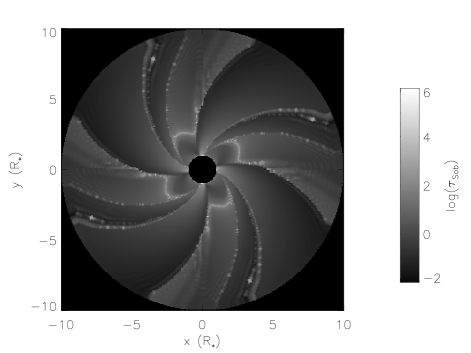
(a) Model 1A

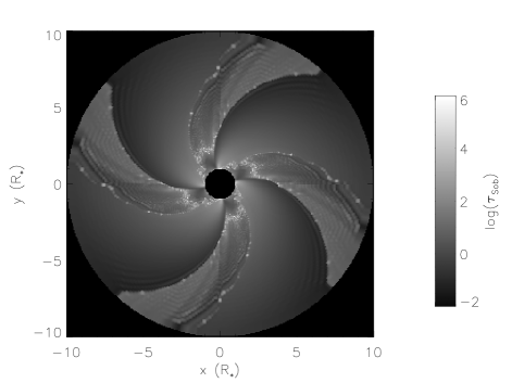
(b) Model 1B

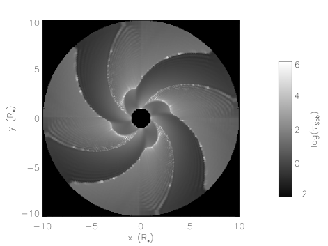
(c) Model 2A

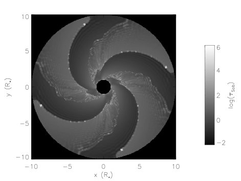
(d) Model 2B

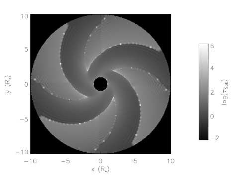
(e) Model 3A

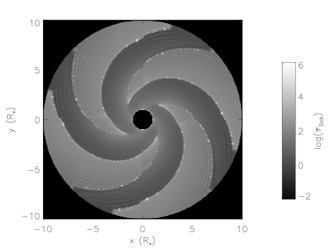
(f) Model 3B

Figure 5: Equatorial plane greyscale visualizations of $\log(\tau_{\textrm{Sob}})$, the Sobolev (radial) optical depth, indicating where in the wind the absorption occurs in each model.

Models 1A and 1B lead to particularly interesting structures: the curvature of the inner edge of the CIRs is very pronounced in the inner wind. This suggests that the extremely overluminous spots overload the wind so strongly that material would perhaps fall back onto the star if it were not for the “boost” provided by the adjacent spot as the star rotates. This behaviour might therefore be a consequence of the chosen number of spots and the associated boundary conditions. However, an investigation of the influence of different spot distributions on this phenomenon is not within the scope of this study. We also notice that the larger, weaker spots produce absorption further from the stellar surface. Therefore, in terms of reproducing the observed properties of DACs, there is a trade-off between having spots that are large enough to produce wind structures that cover a significant fraction of the stellar disk near the surface, and brightness contrasts that are strong enough to overload the wind in such a way that the velocity kinks (or breaks in the radial velocity profile when the acceleration becomes null or negative which are responsible for the DACs, Cranmer & Owocki 1996) are close enough to the surface that their absorption is noticeable.

3.2 Synthetic line profiles

Finally, we compute synthetic resonance line profiles for each of our 6 models. To reduce calculation time, we only computed 14 different phases over a quarter of a rotation period, and then since our simulations are in steady-state, plotted them twice to show two structures evolving in the dynamic spectra. Then, we approximate a “least-absorption” template spectrum, which corresponds roughly to the expected profile without the extra absorption caused by the CIRs (Prinja, Howarth & Henrichs, 1987), by using the maximum value of intensity among the 14 phases for each velocity bin. This constitutes our reference spectrum, by which we divide each spectrum to obtain a quotient spectrum, which is plotted against phase to create our dynamic spectra, following the usual procedure used to visualize DACs in observational data (e.g., Kaper et al. 1996).

Once the dynamic quotient spectra are computed, we compare their characteristics with those of observed UV resonance line profiles from $\xi$ Persei. In particular, we base our comparison on the quantitative analysis performed by Kaper et al. (1999). Their figure 6 shows that the DACs’ maximum depth (or the minimum quotient flux) is about 20-30%, and their figures 7 and 8 show that the DACs typically first appear in the profiles at about one-half the terminal velocity.

The results of our SEI calculations are shown in Figs. 6 to 8. The terminal velocity that is shown on these figures and that is used as a scaling parameter to express the velocity range is estimated from the least-absorption template, in a manner aimed at best reproducing the observational procedure. Since this template was constructed using the maximum value of flux for each velocity bin, some structures extend slightly beyond the inferred terminal velocity. However, this does not particularly affect the scaling of the wind since the underestimation of the terminal velocities is small compared to the terminal velocities themselves.

A first immediate conclusion derived from Figs. 6 to 8 is that not all models produce line profile variations that are qualitatively compatible with those observed in the UV resonance lines of $\xi$ Persei. Indeed, models 1A and 1B produce DACs that are morphologically quite different from those that are observed: unlike $\xi$ Persei’s DACs, rather than getting narrower as they migrate towards terminal velocity, they remain very broad. Furthermore, the observed DACs accelerate at a decreasing rate as they evolve through the velocity space to approach an “asymptotic velocity”; in our case, models 1A and 1B lead to DACs accelerating at an almost constant rate, extending into the blue edge of the line profile as the entire velocity structure of the wind is perturbed. This is somewhat unsurprising, given the peculiar structures revealed in the equatorial plane optical depth plots of the winds of both of these models (Fig. 5). This finding might also be in line with the conclusion of Massa & Prinja (2015) that the spots responsible for DACs must cover some significant portion of the stellar disk.

The remaining 4 models seem to reproduce the DAC behaviour adequately. This is quite remarkable, especially for models 3A and 3B since, as mentioned earlier, the density and velocity structures found in the wind are rather subtle, which illustrates very well the conclusion of Cranmer & Owocki (1996): that DACs are formed by velocity kinks, not by overdense regions in the wind.

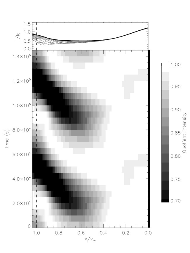
(a) Model 1A synthetic line profile.

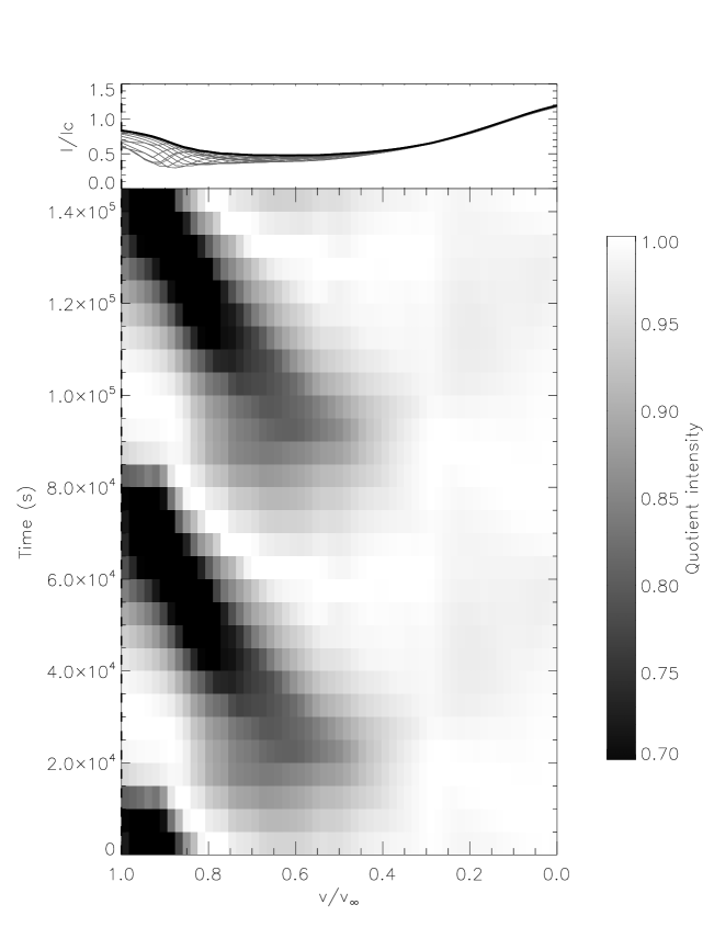
(b) Model 1B synthetic line profile.

Figure 6: Left: Dynamic spectrum (bottom panel) showing synthetic line profiles generated from model 1A (shown in the top panel in grey) divided by a “least-absorption” template spectrum (shown in the top panel in black). The dashed black line represents $v_{\infty}$. Right: Same, but for model 1B. These dynamic spectra illustrate the fact that models 1A and 1B do not appear to appropriately reproduce the observed DAC behaviour.

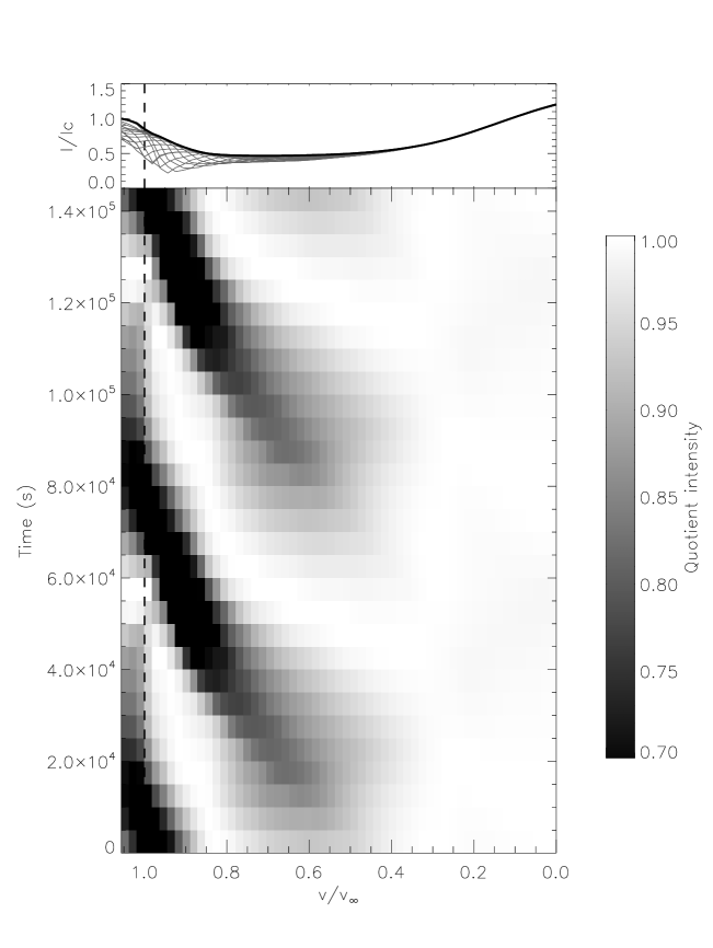
(a) Model 2A synthetic line profile.

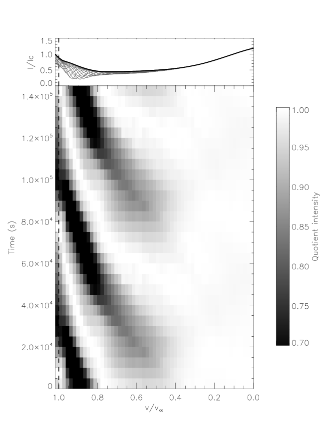
(b) Model 2B synthetic line profile.

Figure 7: Same as Fig. 6, but for models 2A and 2B. In this case, the DACs behave in a way that is compatible with observations: as they approach terminal velocity, their acceleration decreases and they become narrower.

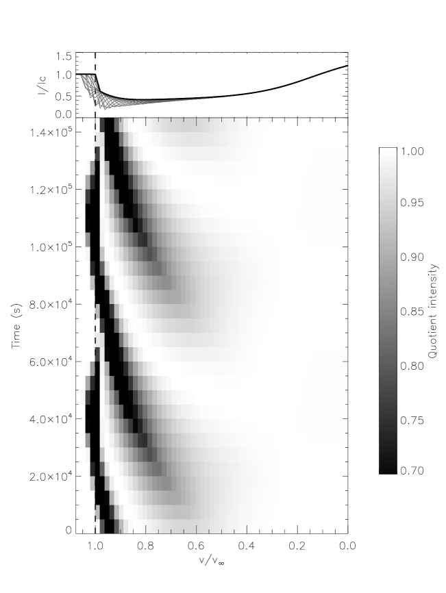
(a) Model 3A synthetic line profile.

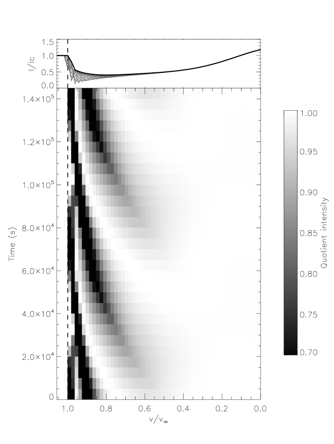
(b) Model 3B synthetic line profile.

Figure 8: Same as Fig. 6, but for models 3A and 3B.

As to the quantitative behaviour of these DACs, we see that for models 2A, 2B, 3A and 3B (Figs. 7 and 8) DACs first appear at about one-half the terminal velocity. However, to better describe their behaviour, we can use the DAC-fitting method used by Henrichs et al. (1983) and Kaper et al. (1999) by fitting a Gaussian absorption profile to each absorption feature in the quotient spectra:

$$I(v)=\exp\left(-\tau_{c}\exp\left[-\left(\frac{v-v_{c}}{v_{t}}\right)^{2}\right]\right)\,,$$ (7)

where $v_{c}$ corresponds to the central velocity of the feature, $v_{t}$ corresponds to its width and $\tau_{c}$ is the central optical depth. This has the additional advantage that we infer the behaviour of DACs in our theoretical spectra using the same method of measurement as used for the observations. We only apply this method to the four models which successfully reproduce DAC behaviour: indeed, not only is the DAC morphology at the blue edge of the line profile problematic for models 1A and 1B, but we found that their DACs are much more non-Gaussian than those of other models throughout the velocity space, and as such, much more difficult to model using this approach. Accordingly, we decided to forgo this analysis for models 1A and 1B.

We find the absorption feature for each model that appears at the lowest velocity across all phases and consider that velocity to be the starting velocity of the DACs (expressed as a fraction of the terminal velocity of the reference spectrum in Table 3). More specifically, a DAC is considered to “appear” for the first time when it becomes discrete, i.e., when it can be fully isolated (or in other words when the profile returns to the continuum on either side of the absorption feature). The starting velocities might be slightly underestimated due to the chosen temporal resolution, but, in the context of this fitting method, the very small values of central optical depth measured when they first appear suggests that this effect is very modest as they cannot have appeared much earlier or they would not have been observable. Therefore, we consider our current time sampling to be adequate. An example of a spectrum in which this first happens (and the fitted DACs) is shown in Fig. 9.

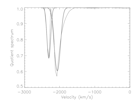
Figure 9: Example of the “appearance” of a DAC (seen here at about $v=1100$ km/s) in model 3A. This corresponds to the first spectrum in which this DAC is discrete and isolated. Two other, “older” DACs can be seen to still exist in the profile. The fits to the DACs correspond to the thick gray lines; note that the higher velocity DACs are not perfectly fit since they are not fully described by Gaussian curves.

The starting velocities reported in Table 3 are compatible with those found for $\xi$ Persei by Kaper et al. (1999). Following their analysis, we can also trace the evolution of the 3 quantities appearing in Eq. 7 for a single DAC caused by a CIR wrapping around the star. Fig. 10 shows the results of these calculations, respectively for $v_{c}$, $\tau_{c}$ and $v_{t}$.

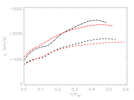
(a) DAC central velocity ($v_{c}$)

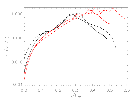
(b) DAC central optical depth ($\tau_{c}$)

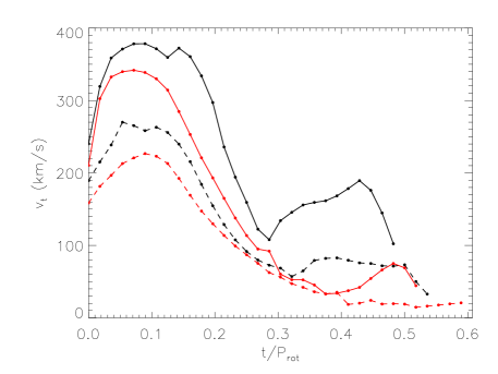
(c) DAC width ($v_{t}$)

Figure 10: Characteristics of the DACs as a function of time; the black curves correspond to model 2 and the red curves to model 3. Full curves correspond to the “A” variety of each model (not including ionization effects) and the dashed curves correspond to the “B” variety (including ionization effects). For all three panels, the horizontal axis corresponds to the time elapsed since the “appearance” of the DAC, as a fraction of the rotation period.

The fit parameters of our synthetic DACs show clear trends: the DACs become stronger and narrower as they evolve through the velocity space. These trends are less clear at low and near-terminal velocity. When the DACs first form, there is significant asymmetry in their profile, leading to unsatisfactory fits using a purely Gaussian profile; furthermore, it is more difficult to fit weak features. When they are near terminal velocity, the departures from the trends are due in part to the finite simulation range, which truncates the CIRs which cause these features. “Quasi-blending” also becomes an issue towards terminal velocity, as two DACs nearly overlap in velocity range, causing slight problems with the fit.

Finally, the maximum depth of the quotient dynamic spectrum for each model is compiled in Table 3. Once again, these values are compatible with the observed values, which range between about 20 and 30%. There seems to be a slight trend between maximum depth and spot size; larger spots lead to somewhat deeper DACs. This might bear interesting consequences for a few other stars in the Kaper et al. (1996) sample, which had nearly saturated DACs. In order to achieve such deep DACs, the wind structures causing the absorption probably have to originate from very large surface spots (in accordance with Massa & Prinja 2015), unless the stars in question exhibit a larger photometric variability than $\xi$ Persei.

In conclusion, by fitting our DACs using the same method used for the observed spectra of $\xi$ Persei, we conclude that the DACs produced by four of our models (2A, 2B, 3A and 3B) have quantitative properties that are very similar to those of $\xi$ Persei’s DACs.

3.3 Effect of ionization

The most obvious effect observed when the ionization parameter $\delta$ is introduced is a global reduction of the wind velocity (as illustrated in Fig. 4), as well as an increase in the mass-loss rate (see Table 3). We also see from Fig. 5 that including a non-zero ionization parameter increases the optical depth of the CIRs and results in their appearance closer to the stellar surface. However, the inclusion of this effect barely influences the computed line profiles. The main reason for this lies in the fact that for a strong UV resonance line, the absorption is nearly saturated at low velocities, making it difficult to distinguish any additional absorption. Indeed, looking at a typical unperturbed profile, we see that the absorption is already nearly saturated at about $v/v_{\infty}=0.3$ (as shown in Fig. 2). We do notice that, in Table 3, the ‘B’ models typically have slightly deeper absorption than the corresponding ‘A’ models, but that effect is very small. The DACs produced in the ‘B’ models are also systematically narrower than their counterparts computed from the ‘A’ models, but once again this is not very surprising since the entire velocity structure of the wind is scaled to a lower terminal velocity. Modelling weaker resonance lines, as well as excited state lines (such as those investigated by Massa & Prinja 2015), might help in the future to define the role of the ionization parameter in our simulations.

4 Conclusions and future work

In this study, we have carried out 2D radiation hydrodynamical simulations of $\xi$ Persei’s wind and aimed to explore whether bright spots compatible with recent observation could be responsible for its observed DACs. The spot characteristics were constrained by the photometric limits found by Ramiaramanantsoa et al. (2014). We then extrapolated these results to 3D using the same prescription as CO96 and used SEI to generate UV resonance line profiles. This procedure allowed us to test whether various spot and wind parameters produced qualitatively similar wind structures, and whether the associated spectroscopic signatures were consistent with the DAC phenomenology. We used three sets of spot parameters (size and amplitude), each of which was then tested with or without including the effects of the radial dependence of ionization levels in the wind. Based on these experiments, we conclude the following:

• All 6 spot models cause perturbations in the velocity and density profiles of the wind. Models with smaller and stronger spots cause structures with larger overdensities and velocity plateaus in the wind, while larger and weaker spots generate subtler structures. The hydrodynamical simulations also show evidence that the spots enhance the overall mass-loss rate and that, as expected, the inclusion of the effect of radially-varying ionization globally slows down the wind and increases mass loss, leading to stronger absorption in the CIRs.

• The synthetic line profiles show classical DAC behaviour for 4 out of the 6 models. The quantitative behaviour of the DACs also agrees with observations: they appear at a little less than one-half the terminal velocity, then become deeper and narrower as they evolve in the velocity space, reaching a maximum depth of around 30% for model 2A, going down to about 20% for model 3B. Thus, the key result of this study is that we have successfully linked the behaviours of two sets of observations, i.e., optical photometry and UV spectroscopy, within the “bright spot paradigm” introduced by CO96 by using $\xi$ Persei as a testbed.

• The fact that models corresponding to a range of spot sizes reproduce the pattern of variability associated with DACs suggests that there can exist a variety of these structures in the wind of $\xi$ Persei at different times, since there is no reason to favour one model over the other (and the quality of the existing data might not allow us at this point to distinguish between these). However, our results also eliminate some portions of the parameter space, thus allowing us to constrain this problem. If we accept the idea that these structures are generated by bright spots on the surface of the star, we deem our findings to be compatible with the idea that these spots are stochastic, appearing and disappearing over time, with varying strengths and sizes. Such a scenario might explain the cyclical (rather than periodic) nature of DACs.

The main limitation of this study is that we have not convincingly addressed the role of the ionization factor in producing DACs. While its effect on the global properties of the wind was quite obvious (and unsurprising), its inclusion did not seem to be a significant factor when it comes to the DACs’ properties. Further investigation will be required in order to clarify this issue.

As to the nature of the physical phenomenon giving rise to these spots, the present work helps place lower limits on the strength that magnetic spots (e.g., Cantiello & Braithwaite 2011) would need to have to produce the appropriate brightness enhancements. Using Eq. 5 from David-Uraz et al. (2014) and assuming $\log(g)=3.5$, we approximate that the field strength required to generate the brightness contrast used in model 2 is 360 G, whereas model 3 requires a 160 G field. Assuming a best case scenario involving a spot situated in the center of the disk, and taking the field to be along the line of sight at each point (which is a valid approximation given the size of the spots), we expect to measure disk-averaged longitudinal fields of, respectively, 11 G and 19 G. Such fields could be detectable using deep magnetometry; currently, the best longitudinal field error bar obtained for $\xi$ Persei using NARVAL observations is 21 G (David-Uraz et al., 2014). For a given photometric variation constraint, larger spots would therefore yield larger longitudinal field values. However, as seen throughout Section 3, larger spots lead to weaker CIRs, and the extra absorption they cause occurs further away from the star, which might be at odds with various other observational diagnostics, including excited state lines (Massa & Prinja, 2015).

The best way to compute the behaviour of wind structures near the stellar surface would therefore be to generate synthetic line profiles that are more sensitive to that region of the wind. Another important observable to investigate would also be the behaviour of H$\alpha$. Indeed, variations in H$\alpha$ are known to be linked to DACs, but their patterns typically do not look as well organized as that of their UV counterparts. Nevertheless, since high-resolution optical spectroscopy is much more accessible than UV spectroscopy these days, it would be very useful to make sense of these patterns and determine whether they allow us to infer anything about the surface perturbations which cause them.

Another extension of this study would be to investigate if our modeled CIRs can account for the X-ray variability observed in a number of O stars, such as $\lambda$ Cephei (Rauw et al., 2015). Currently our simulations are isothermal: we would need to track the temperature structure of the wind and ideally produce 3D models to fully account for the modulation of the X-ray absorption by large-scale structures such as CIRs.

Finally, while this paper self-consistently accounts for the behaviour of two observables within a “CO96-like” paradigm for a specific star, future work should extend the parameter space to account for the great variety of DAC signatures found in all OB stars, not just $\xi$ Persei.

References

- Abbott (1982) Abbott D.C., 1982, ApJ, 259, 282
- Cantiello & Braithwaite (2011) Cantiello M., Braithwaite J., 2011, A&A, 534, A140
- Castor, Abbott & Klein (1975) Castor J.I., Abbott D.C., Klein R.I., 1975, ApJ, 195, 157
- Chené et al. (2011) Chené A.-N., Moffat A.F.J., Cameron C., Fahed R., Gamen R.C., Lefèvre L., Rowe J.F., St-Louis N., Muntean V., de la Chevrotière A., Guenther D.B., Kuschnig R., Matthews J.M., Rucinski S.M., Sasselov D., Weiss W.W., 2011, ApJ, 735, 34
- Colella & Woodward (1984) Colella P., Woodward P.R., 1984, J. Comp. Phys., 54, 174
- Cranmer & Owocki (1995) Cranmer S.R., Owocki S.P., 1995, ApJ, 440, 308
- Cranmer & Owocki (1996) Cranmer S.R., Owocki S.P., 1996, ApJ, 462, 469
- David-Uraz et al. (2012) David-Uraz A., Moffat A.F.J., Chené A.-N., Rowe J.F., Lange N., Guenther D.B., Kuschnig R., Matthews J.M., Rucinski S.M., Sasselov D., Weiss W.W., 2012, MNRAS, 426, 1720
- David-Uraz et al. (2014) David-Uraz A., Wade G.A., Petit V., ud-Doula A., Sundqvist J.O., Grunhut J., Shultz M., Neiner C., Alecian E., Henrichs H.F., Bouret J.-C., MiMeS Collaboration, 2014, MNRAS, 444, 429
- de Jong et al. (1999) de Jong J.A., Henrichs H.F., Schrijvers C., Gies D.R., Telting J.H., Kaper L., Zwarthoed G.A.A., 1999, A&A, 345, 172
- de Jong et al. (2001) de Jong J.A., Henrichs H.F., Kaper L., Nichols J.S., Bjorkman K., Bohlender D.A., Cao H., Gordon K., Hill G., Jiang Y., Kolka I., Morrison N., Neff J., O’Neal D., Scheers B., Telting J.H., 2001, A&A, 368, 601
- Dessart (2004) Dessart L., 2004, A&A, 423, 693
- Fullerton et al. (1997) Fullerton A.W., Massa D.L., Prinja R.K., Owocki S.P., Cranmer S.R., 1997, A&A, 327, 699
- Gayley (1995) Gayley K.G., 1995, ApJ, 454, 410
- Hamann (1981) Hamann W.-R., 1981, A&A, 93, 353
- Haser et al. (1995) Haser S.M., Lennon D.J., Kudritzki R.P., Puls J., Pauldrach A.W.A., Bianchi L., Hutchings J.B., 1995, A&A, 295, 136
- Henrichs et al. (1983) Henrichs H.F., Hammerschlag-Hensberge G., Howarth I.D., Barr P., 1983, ApJ, 268, 807
- Howarth & Prinja (1989) Howarth I.D., Prinja R.K., 1989, ApJS, 69, 527
- Kaper et al. (1996) Kaper L., Henrichs H.F., Nichols J.S., Snoek L.C., Volten H., Zwarthoed G.A.A., 1996, A&AS, 116, 257
- Kaper et al. (1997) Kaper L., Henrichs H.F., Fullerton A.W., Ando H., Bjorkman K.S., Gies D.R., Hirata R., Kambe E., McDavid D., Nichols J.S., 1997, A&A, 327, 281
- Kaper et al. (1999) Kaper L., Henrichs H.F., Nichols J.S., Telting J.H., 1999, A&A, 344, 231
- Kee (2015) Kee N.D., 2015, PhD dissertation, University of Delaware
- Krtička & Kubát (2010) Krtička J., Kubát J., 2010, A&A, 519, A50
- Lamers, Cerruti-Sola & Perinotto (1987) Lamers H.J.G.L.M., Cerruti-Sola M., Perinotto M., 1987, ApJ, 314, 726
- Lamers & Leitherer (1993) Lamers H.J.G.L.M., Leitherer C., 1993, ApJ, 412, 771
- Marcolino et al. (2013) Marcolino W.L.F., Bouret J.-C., Sundqvist J.O., Walborn N.R., Fullerton A.W., Howarth I.D., Wade G.A., ud-Doula A., 2013, MNRAS, 431, 2253
- Massa & Prinja (2015) Massa D., Prinja R.K., 2015, ApJ, 809, 12
- Mullan (1986) Mullan D.J., 1986, A&A, 165, 157
- Owocki et al. (1988) Owocki S.P., Castor J.I., Rybicki G.B., 1988, ApJ, 335, 914
- Owocki, Cranmer & Fullerton (1995) Owocki S.P., Cranmer S.R., Fullerton A.W., 1995, ApJ, 453, L37
- Owocki (1999) Owocki S.P., 1999, in Variable and Non-spherical Stellar Winds in Luminous Hot Stars, Proceedings of the IAU Colloquium No. 169 held in Heidelburg, Germany, eds. Wolf B., Stahl O., Fullerton A.W., Lecture Notes in Physics, 523, 294
- Prinja (1988) Prinja R.K., 1988, MNRAS, 231, 21
- Prinja & Howarth (1986) Prinja R.K., Howarth I.D., 1986, ApJS, 61, 357
- Prinja, Howarth & Henrichs (1987) Prinja R.K., Howarth I.D., Henrichs H.F., 1987, ApJ, 317, 389
- Puls, Owocki & Fullerton (1993) Puls J., Owocki S.P., Fullerton A.W., 1993, A&A, 279, 457
- Puls, Springmann & Lennon (2000) Puls J., Springmann U., Lennon M., 2000, A&AS, 141, 23