Clustering Small Samples with Quality Guarantees:
Adaptivity with One2all pps

Abstract

Clustering of data points is a fundamental tool in data analysis. We consider points $X$ in a relaxed metric space, where the triangle inequality holds within a constant factor. A clustering of $X$ is a partition of $X$ defined by a set of points $Q$ (centroids), according to the closest centroid. The cost of clustering $X$ by $Q$ is $V(Q)=\sum_{x\in X}d_{xQ}$. This formulation generalizes classic $k$-means clustering, which uses squared distances. Two basic tasks, parametrized by $k\geq 1$, are cost estimation, which returns (approximate) $V(Q)$ for queries $Q$ such that $|Q|=k$ and clustering, which returns an (approximate) minimizer of $V(Q)$ of size $|Q|=k$. With very large data sets $X$, we seek efficient constructions of small samples that act as surrogates to the full data for performing these tasks. Existing constructions that provide quality guarantees are either worst-case, and unable to benefit from structure of real data sets, or make explicit strong assumptions on the structure. We show here how to avoid both these pitfalls using adaptive designs.

At the core of our design is the novel one2all construction of multi-objective probability-proportional-to-size (pps) samples: Given a set $M$ of centroids and $\alpha\geq 1$, one2all efficiently assigns probabilities to points so that the clustering cost of each $Q$ with cost $V(Q)\geq V(M)/\alpha$ can be estimated well from a sample of size $O(\alpha|M|\epsilon^{-2})$. For cost queries, we can obtain worst-case sample size $O(k\epsilon^{-2})$ by applying one2all to a bicriteria approximation $M$, but we adaptively balance $|M|$ and $\alpha$ to further reduce sample size. For clustering, we design an adaptive wrapper that applies a base clustering algorithm to a sample $S$. Our wrapper uses the smallest sample that provides statistical guarantees that the quality of the clustering on the sample carries over to the full data set. We demonstrate experimentally the huge gains of using our adaptive instead of worst-case methods.

1 Introduction

Clustering is a fundamental and prevalent tool in data analysis. We have a set $X$ of data points that lie in a (relaxed) metric space $(\mathcal{M},d)$, where distances satisfy a relaxed triangle inequality: For some constant $\rho\geq 1$, for any three points $x,y,z$, $d_{xy}\leq\rho(d_{xz}+d_{zy})$. Note that any metric space with distances replaced by their $p$th power satisfies this relaxation: For $p\leq 1$ it remains a metric and otherwise we have $\rho=2^{p-1}$. In particular, for squared distances ($p=2$), commonly used for clustering, we have $\rho=2$.

Each set $Q\subset\mathcal{M}$ of points (centroids) defines a clustering, which is a partition of $X$ into $|Q|$ clusters, which we denote by $X_{q}$ for $q\in Q$, so that a point $x\in X$ is in $X_{q}$ if and only if it is in the Voronoi region of $q$, that is $q=\arg\min_{y\in Q}d_{xy}$. We allow points $x\in X$ to have optional weights $w_{x}>0$, and define the cost of clustering $X$ by $Q$ to be

$$V(Q\mid X,\boldsymbol{w})=\sum_{x\in X}w_{x}d_{xQ}\ ,$$ (1)

where $d_{xQ}=\min_{y\in Q}d_{xy}$ is the distance from point $x$ to the set $Q$.

Two fundamental computational tasks are cost queries and clustering (cost minimization). The clustering cost (1) of query $Q$ can be computed using $n|Q|$ pairwise distance computations, where $n=|X|$ is the number of points in $X$. With multiple queries, it is useful to pre-process $X$ and return fast approximate answers. Clustering amounts to finding $Q$ of size $|Q|\leq k$ with minimum cost:

$$\arg\min_{Q\mid|Q|\leq k}V(Q\mid X,\boldsymbol{w})\ .$$ (2)

Optimal clustering is computationally hard [3] even on Euclidean spaces and even to tightly approximate [5]. There is a local search polynomial algorithm with $9+\epsilon$ approximation ratio [21]. In practice, clustering is solved using heuristics, most notably Lloyd’s algorithm (EM) for squared Euclidean distances [24] and scalable approximation algorithms such as kmeans++ [4] for general metrics. EM iterates allocating points to clusters defined by the nearest centroid, and replacing each centroid with the center of mass $\sum_{x}w_{x}x$ of its cluster. Each iteration uses $|X|k$ pairwise distance computations. It is a heutistic because although each iteration reduces the clustering cost, the algorithm can terminates in a local minima. kmeans++ produces a sequence of points $\{m_{i}\}$: The first point $m_{1}$ is selected randomly with probability $\propto w_{x}$ and a point $m_{i}$ us selected with probability $\propto w_{x}d_{\{m_{1},\ldots,m_{i-1}\}x}$. Each iteration requires $O(|X|)$ pairwise distance computations. kmeans++ guarantees that the expected clustering cost of the first $k$ points is within an $O(\log k)$ factor of the optimum $k$-means cost. Moreover, kmeans++ provides bi-criteria guarantees [2, 29]: The first $\beta k$ points selected (for some constant $\beta>1$) have expected clustering cost is within a constant factor of the optimum $k$-means cost. In practice, kmeans++ is often used to initiallize Lloyd’s algorithm.

When the set of points $X$ is very large, we seek an efficient method that computes a small summary structure that can act as a surrogate to the full data sets and allow us to efficiently approximate clustering costs. These structures are commonly in the form of subsets $S\subset X$ with weights $\boldsymbol{w}^{\prime}$ so that $V(Q\mid S,\boldsymbol{w}^{\prime})$ approximates $V(Q\mid X,\boldsymbol{w})$ for each $Q$ of size $k$. Random samples are a natural form of such structures. The challenge is, however, that we need to choose the weights carefully: A uniform sample of $X$ always provide us with unbiased estimates of clustering costs but can miss critical points and will not provide quality guarantees.

When designing summary structures, we seek to optimize the tradeoff between the structure size and the quality guarantees it provides. The term coresets for such summary structures was coined in the computational geometry literature [1, 19], building on the theory of $\epsilon$-nets. Some notable coreset constructions include [25, 10, 16, 17]. Early coresets constructions had bounds with high (exponential or high polynomial) dependence on some parameters (dimension, $\epsilon$, $k$) and poly logarithmic dependence on $n$. The state-of-the-art asymptotic bound of $O(k\epsilon^{-2}\log k\log n)$ is claimed in [6].

The bulk of coreset constructions are aimed to provide strong “ForAll” statistical guarantees, which bound the distribution of the maximum approximation error of all $Q$ of size $k$. The ForAll requirement, however, comes with a hefty increase in structure size and is an overkill for the two tasks we have at hand: For clustering cost queries, weaker per-query “ForEach” typically suffice, which for each $Q$, with very high probability over the structure distribution, bound the error of the estimate of $V(Q)$. For clustering, it suffices to guarantee that the (approximate) minimizers of $V(Q\mid S,\boldsymbol{w}^{\prime})$ are approximate minimizers of $V(Q\mid X,\boldsymbol{w})$. Moreover, previous constructions use coreset sizes that are worst-case, based on general (VC) dimension or union bounds. Even when a worst-case bound is tight up to constants, which typically it is not (constants are not even specified in state of the art coreset constructions), it only means it is tight for pathological data sets of the particular size and dimension. A much smaller summary structure might suffice when there is structure typical in data such as natural clusterability (which is what we seek) and lower dimensionality than the ambient space.

It seems on the surface, however, that in order to achieve statistical guarantees on quality of the results one must either make explicit assumptions on the data or use the worst-case size. We show here how to avoid both these pitfalls via elegant adaptive designs.

Contribution Overview

Our main building block are novel summary structures for clustering costs based on multi-objective probability-proportional-to-size (pps) samples [14, 12], which build on the classic notion of sample coordination [22, 7, 26, 11].

Consider a particular set $Q$ of centroids. The theory of weighted sampling [27, 28] tells us that to estimate the sum $V(Q\mid X,\boldsymbol{w})$ it suffices to sample $\epsilon^{-2}$ points with probabilities $p_{x}\propto w_{x}d_{Qx}$ proportional to their contribution to the sum [18]. The inverse-probability [20] estimate obtained from the sample $S$,

$$\hat{V}(Q\mid X,\boldsymbol{w})\equiv V(Q\mid S,\{w_{x}/p_{x}\})\ ,$$

is an unbiased estimate of $V(Q\mid X,\boldsymbol{w})$ with well-concentrated (in the Bernstein-Chernoff sense) normalized squared error that is bounded by $\epsilon$. The challenge here for us is that we are interested in simultaneously having pps-like quality guarantees for all subsets $Q$ of size $k$ whereas the estimate $V(Q^{\prime}\mid S,\{w_{x}/p_{x}\})$ when $S$ is taken from a sample distribution according to $Q\not=Q^{\prime}$ will not provide these guarantees for $Q^{\prime}$. To obtain these quality guarantees for all $Q$ by a single sample, we use multi-objective pps sampling probabilities, where the sampling probability of each point $x\in X$ is the maximum pps probability over all $Q$ of size $k$.

Clearly, the size of a multi-objective sample will be larger than that of a dedicated pps sample. Apriori, it seems that the size overhead can be very large. Surprisingly, we show that on any (relaxed) metric space, the overhead is only $O(k)$. That is, a multi-objective pps sample of size $O(k\epsilon^{-2})$ provides, for each $Q$ of size $k$, the same estimate quality guarantees as a dedicated pps sample of size $O(\epsilon^{-2})$ for $Q$. Note that the overhead does not depend on the dimensionality of the space or on the size of the data. Our result generalizes previous work [9] that only applied to the case where $k=1$, where clustering cost reduces to inverse classic closeness centrality (sum of distances from a single point $Q$).

For our applications, we also need to efficiently compute these probabilities – the straightforward method of enumerating over the infinite number of subsets $Q$ is clearly not feasible. Our main technical contribution, which is the basis of both the existential and algorithmic results, is an extremely simple and very general construction which we refer to as one2all: Given a set $M$ of points and any $\alpha\geq 1$, we compute using $|M|n$ distance computation sampling probabilities for points in $X$ that upper bound the multi-objective sampling probabilities for all subset $Q$ with clustering cost $V(Q)\geq V(M)/\alpha$. Moreover, the overhead is only $O(\alpha|M|)$.

By considering the one2all probabilities for an optimal clustering $M$ of size $k$ and $\alpha=1$, we establish existentially that a multi-objective pps sample for all sets $Q$ of size $k$ has size $O(k\epsilon^{-2})$. To obtain such probabilities efficiently, we can apply kmeans++ [4] or another efficient bi-criteria approximation algorithm to compute $M$ of size $\beta k$ (for a small constant $\beta$) that has cost within a factor of $\alpha>1$ than the optimum $k$-clustering [29]. We then compute one2all probabilities for $M$ and $\alpha$.

This, however, is a worst-case construction. We further propose a data-adaptive enhancement that can decrease sample size significantly while retaining the quality guarantees: Note that instead of applying one2all to $(M,\alpha)$, we can instead use $M^{\prime}\subset M$ and $\alpha^{\prime}\leftarrow\alpha V(M^{\prime})/V(M)$. Our adaptive design uses the sweet-spot prefix $M^{\prime}$ of the centroids sequence returned by kmeans++ that minimizes the sample size.

For the task of approximate cost queries, we pre-process the data as above to obtain multi-objective pps probabilities and compute a sample $S$ with size parameter $\epsilon^{-2}$. We then process cost queries $Q$ by computing and returning the clustering cost of $S$ by $Q$: $V(Q\mid S,\{w_{x}/p_{x}\})$. Each computation performs $O(|S||Q|)$ pairwise distance computations instead of the $O(n|Q|)$ that would have been required over the full data. This can be further reduced using approximate nearest neighbor structures. Our estimate provides pps statistical guarantees for each $Q$ of size $k$, or more generally, for each $Q$ with $V(Q\mid X,\boldsymbol{w})\geq V(M\mid X,\boldsymbol{w})/\alpha$. Note that both storage and query computation are linear in the sample size. The worst-case sample size is $O(\alpha|M|\epsilon^{-2})=O(k\epsilon^{-2})$ but our adaptive design can yield much smaller samples.

For the task of approximate clustering, we adapt an optimization framework over multi-objective samples [12]. The meta algorithm is a wrapper that inputs multi-objective pps probabilities, specified error guarantee $\epsilon$, and a black-box (exact, approximate, bicriteria, heuristic) base clustering algorithm $\mathcal{A}$. The wrapper applies $\mathcal{A}$ to a sample to obtain a respective approximate minimizer of the clustering cost over the sample. When the sample is much smaller than the full data set, we can expect better clustering quality using less computation. Our initial multi-objective pps sample provides ForEach guarantees that apply to each estimate in isolation but not to the sample optimum. In particular, it does not guarantee us that the solution over the sample has the respective quality over the full data set. A larger sample may or may not be required. One can always increase the sample by a worst-case upper bound (using a union bound or domain-specific dimensionality arguments). Our adaptive approach exploits a critical benefit of ForEach: That is, we are able to test the quality of the sample approximate optimizer $Q$ returned by $\mathcal{A}$: If the clustering cost of $V(Q\mid X,\boldsymbol{w})$ agrees with the estimate $V(Q\mid S,\boldsymbol{w}^{\prime})$ then we can certify that $Q$ has similar (within $(1+\epsilon)$ quality over $X$ as it has over the sample $S$. Otherwise, the wrapper doubles the sample size $S$ and repeats until the test is satisfied. Since the base algorithm is always at least linear, the total computation is dominated by that last largest sample size we use.

Note that the only computation performed over the full data set are the $O(k)$ iterations of kmeans++ that produce $(M,\alpha)$ to which we apply one2all. Each such iteration performs $O(|X|)$ distance computations. This is a significant gain, as even with Lloyd’s algorithm (EM heuristic), each iteration is $O(k|X|)$. This design allows us to apply more computationally intensive $\mathcal{A}$ to a small sample.

A further adaptive optimization targets this initial cost: On real-world data it is often the case that much fewer iterations of kmeans++ bring us to within some reasonable factor $\alpha$ of the optimal $k$-clustering. We thus propose to adaptively perform additional kmeans++ iterations as to balance their cost with the size of the sample that we need to work with.

We demonstrate through experiments on both synthetic and real-world data the potentially huge gains of our data-adaptive method as a replacement to worst-case-bound size samples or coresets.

The paper is organized as follows. Pps and multi-objective pps sampling in the context of clustering are reviewed in Section 2. Section 3 presents our one2all probabilities and implications. Section 4 provides a full proof of the one2all Theorem. Section 5 present adaptive clustering cost oracles and Section 6 presents an adaptive wrapper for clustering on samples. Section 7 demonstrated experimentally, using natural synthetic data, the enormous gain by using data-dependent adaptive instead of worst-case sizes.

2 Multi-objective pps samples for clustering

We review the framework of weighted and multi-objective weighted sampling [12] in our context of clustering costs. Consider approximating the clustering cost $V(Q\mid X,\boldsymbol{w})$ from a sample $S$ of $X$. For probabilities $p_{x}>0$ for $x\in X$ and a sample $S$ drawn according to these probabilities, we have the unbiased inverse probability estimator [20] of $V(Q\mid X,\boldsymbol{w})$:

$$\hat{V}(Q\mid X,\boldsymbol{w})=\sum_{x\in S}w_{x}\frac{d_{xQ}}{p_{x}}=V(Q\mid S,\{w_{x}/p_{x}\})\ .$$ (3)

Note that the estimate is equal to the clustering cost of $S$ with weights $w_{x}/p_{x}$ by $Q$.

2.1 Probability proportional to size (pps) sampling

To obtain guarantees on the estimate quality of the clustering cost by $Q$, we need to use weighted sampling [18]. The pps base probabilities of $Q$ for $x\in X$ are

$$\psi_{x}^{(Q\mid X,\boldsymbol{w})}=\frac{w_{x}d_{xQ}}{\sum_{y\in X}w_{y}d_{yQ}}\ .$$ (4)

The pps probabilities for a sample with size parameter $r>1$ are

$$r*\psi_{x}^{(Q\mid X,\boldsymbol{w})}=\min\{1,r\psi_{x}^{(Q\mid X,\boldsymbol{w})}\}\ .$$

Note that the (expected) sample size is $\sum_{x}p_{x}$. When $p_{x}=r*\psi_{x}^{(Q\mid X,\boldsymbol{w})}$, the size is at most $r$. With pps sampling we obtain the following guarantees:

Theorem 2.1 ((weak) pps sampling)

Consider a sample $S$ where each $x\in X$ is included independently (or using VarOpt dependent sampling [8, 13]) with probability $p_{x}\geq\alpha\epsilon^{-2}*\psi_{x}^{(Q\mid X,\boldsymbol{w})}$, where $\alpha\leq 1$. Then the estimate (3) has the following statistical guarantees:

• The coefficient of variation (CV), defined as the ratio of the standard deviation to the mean, (measure of the “relative error”) is at most $\epsilon/\sqrt{\alpha}$.

• The estimate is well concentrated in the Chernoff-Bernstein sense. In particular, we have the following bounds on the relative error:

  $$\text{For $\delta\geq 0$,\ }\Pr[V(Q\mid S)\geq(1+\delta)V(Q\mid X,\boldsymbol{w})]\leq\exp(-\delta\ln(1+\delta)\alpha\epsilon^{-2}/2)$$

  $$\text{For $\delta\leq 1$,\ }\Pr[V(Q\mid S)\leq(1-\delta)V(Q\mid X,\boldsymbol{w})]\leq\exp(-\delta^{2}\alpha\epsilon^{-2}/2)$$

  $$\text{For $\delta\geq 1$,\ }\Pr[V(Q\mid S)\geq(1+\delta)V(Q\mid X,\boldsymbol{w})]\leq\frac{1}{\delta-1}\ .$$

Proof

See for example [12]. To establish the CV bound, note that the per-point contribution to the variance of the estimate is $(1/p_{x}-1)(d_{Qx}w_{x})^{2}\leq\alpha^{-1}\epsilon^{2}V(Q)d_{xQ}w_{x}$. The sum is $\leq\alpha^{-1}\epsilon^{2}V(Q)^{2}$ and the CV is at most $\epsilon/\sqrt{\alpha}$. The stated confidence bounds follow from the simplified multiplicative form of Chernoff bound. The last inequality is Markov’s inequality.  

For our purposes here, we will use the following bound on the probability that with weak pps sampling ($\alpha<1$) the estimate exceeds $\alpha^{-1}V(Q\mid X,\boldsymbol{w})$:

Corollary 2.1 (Overestimation probability)

$$\text{For $\alpha\leq 0.5$,}\ \Pr[V(Q\mid S)\geq\alpha^{-1}V(Q\mid X,\boldsymbol{w})]\leq\min\{\frac{\alpha}{1-2\alpha},\exp(-(1-\alpha)\ln(1/\alpha)\epsilon^{-2}/2)\}$$

Proof

We substitute relative error of $\delta=(1/\alpha-1)$ in the multiplicative Chernoff bounds and by also applying Markov inequality.  

2.2 Multi-objective pps

When we seek estimates with statistical guarantees for a set $\mathcal{Q}$ of queries (for example, all sets of $k$ points in the metric space $\mathcal{M}$), we use multi-objective samples [14, 12]. The multi-objective (MO) pps base sampling probabilities are defined as the maximum of the pps base probabilities over $Q\in\mathcal{Q}$:

$$\psi_{x}^{(\mathcal{Q}\mid X,\boldsymbol{w})}=\max_{Q\in\mathcal{Q}}\psi_{x}^{(Q\mid X,\boldsymbol{w})}\ .$$ (5)

Accordingly, for a size parameter $r$, the multi-objective pps probabilities are

$$r*\psi_{x}^{(\mathcal{Q}\mid X,\boldsymbol{w})}=\min\{1,r\psi_{x}^{(\mathcal{Q}\mid X,\boldsymbol{w})}\}=\max_{Q\in\mathcal{Q}}r*\psi_{x}^{(Q\mid X,\boldsymbol{w})}\ .$$

A key property of multi-objective pps is that the CV and concentration bounds of dedicated (weak) pps samples (Theorem 2.1 and Corollary 2.1) hold. We refer to these multi-objective statistical quality guarantees as “ForEach,” meaning that they hold for each $Q$ over the distribution of the samples. We define the overhead of multi-objective sampling $\mathcal{Q}$ or equivalently of the respective base probabilities as:

$$h(\mathcal{Q}\mid X,\boldsymbol{w})\equiv|\boldsymbol{\psi}^{(\mathcal{Q}\mid X,\boldsymbol{w})}|_{1}\equiv\sum_{x\in X}\psi_{x}^{(\mathcal{Q}\mid X,\boldsymbol{w})}\ .$$

Note that the overhead is always between $1$ and $|\mathcal{Q}|$. The overhead bounds the factor-increase in sample size due to “multi-objectiveness:” The multi-objective pps sample size with size parameter $r$ is at most $|r*\psi^{(Q\mid X,\boldsymbol{w})}|_{1}\leq rh(\mathcal{Q}\mid X,\boldsymbol{w})$.

Sometimes we can not compute $\boldsymbol{\psi}$ exactly but can instead efficiently obtain upper bounds $\boldsymbol{\pi}\geq\boldsymbol{\psi}^{(\mathcal{Q}\mid X,\boldsymbol{w})}$. Accordingly, we use sampling probabilities $r*\boldsymbol{\pi}$. The use of upper bounds increases the sample size. We refer to $h(\boldsymbol{\pi})=|\boldsymbol{\pi}|_{1}$ as the overhead of $\boldsymbol{\pi}$. We seek upper-bounds $\boldsymbol{\pi}$ with overhead not much larger than $h(\mathcal{Q}\mid X,\boldsymbol{w})$.

3 one2all probabilities

Consider a relaxed metric space $(\mathcal{M},d)$ where distances satisfy all properties of a metric space except that the triangle inequality is relaxed using a parameter $\rho\geq 1$:

$$\forall x,y,z\in\mathcal{M},\ d_{xy}\leq\rho(d_{xz}+d_{zy})\ .$$ (6)

Let $(X,\boldsymbol{w})$ where $X\subset\mathcal{M}$ and $\boldsymbol{w}>0$ be weighted points in $\mathcal{M}$. For another set of points $M\subset\mathcal{M}$, which we refer to as centroids, and $q\in M$, we denote by

$$X^{(M)}_{q}=\{x\in X\mid d_{xq}=d_{xM}\}$$

the points in $X$ that are closest to centroid $q$. In case of ties we apply arbitrary tie breaking to ensure that $X^{(M)}_{q}$ for $q\in M$ forms a partition of $X$. We will assume that $X^{(M)}_{q}$ is not empty for all $q\in M$, since otherwise, we can remove the point $q$ from $M$ without affecting the clustering cost of $X$ by $M$.

Our one2all construction takes one set of centroids $M$ and computes base probabilities for $x\in X$ such that samples from it allow us to estimate the clustering costs of all $Q$ with estimation quality guarantees that depends on $V(Q\mid X,\boldsymbol{w})$. For a set $M$ we define the one2all base probabilities $\boldsymbol{\pi}^{(M\mid X,\boldsymbol{w})}$ as:

$$\forall m\in M,\ \forall x\in X_{m},$$ (7)

$$\pi^{(M|X,\boldsymbol{w})}_{x} = \min\left\{1,\max\left\{2\rho\frac{w_{x}d_{xM}}{V(M\mid X,\boldsymbol{w})},\frac{8\rho^{2}w_{x}}{w(X_{m})}\right\}\right\}\ .$$

We omit the superscripts when clear from context.

Theorem 3.1 (one2all)

Consider weighted points $(X,\boldsymbol{w})$ in a relaxed metric space with parameter $\rho$, points $M$, and a set $Q$ of centroids. Then

$$\boldsymbol{\pi}^{(M\mid X,\boldsymbol{w})}\geq\min\{1,\frac{V(Q\mid X,\boldsymbol{w})}{V(M\mid X,\boldsymbol{w})}\}\boldsymbol{\psi}^{(Q\mid X,\boldsymbol{w})}\ ,$$

where $\boldsymbol{\pi}^{(M\mid X,\boldsymbol{w})}$ are the one2all base probabilities for $M$.

The full proof of the Theorem is provided in the next section. As a corollary, we obtain that for $r\geq 1$, we can upper bound the multi-objective base pps probabilities $\boldsymbol{\psi}^{(\mathcal{Q}\mid X,\boldsymbol{w})}$ and the overhead $h(\mathcal{Q})$ of the set $\mathcal{Q}$ of all $Q$ with at least a fraction $1/r$ of the clustering cost of $M$:

Corollary 3.1

Consider $M$ and $r\geq 1$ and the set $\mathcal{Q}=\{Q\mid V(Q\mid X,\boldsymbol{w})\geq V(M\mid X,\boldsymbol{w})/r\}$. Then, $r*\boldsymbol{\pi}^{(M\mid X,\boldsymbol{w})}\geq\boldsymbol{\psi}^{(\mathcal{Q}\mid X,\boldsymbol{w})}$ and $h(\mathcal{Q})\leq r(8\rho^{2}|M|+2\rho)$.

Proof

For $Q\in\mathcal{Q}$, $r*\boldsymbol{\pi}^{(M\mid X,\boldsymbol{w})}\geq r\min\{1,\frac{V(Q\mid X,\boldsymbol{w})}{V(M\mid X,\boldsymbol{w})}\}*\boldsymbol{\psi}^{(Q\mid X,\boldsymbol{w})}\geq\boldsymbol{\psi}^{(Q\mid X,\boldsymbol{w})}$. Note that $|\boldsymbol{\pi}^{(M|X,\boldsymbol{w})}|_{1}\leq 8\rho^{2}|M|+2\rho$.  

We can also upper bound the multi-objective overhead of all sets of centroids of size $k$:

Corollary 3.2

For $k\geq 1$, let $\mathcal{Q}$ be the set of all k-subsets of points in a relaxed metric space $\mathcal{M}$ with parameter $\rho$. The multi-objective pps overhead of $\mathcal{Q}$ satisfies

$$h(\mathcal{Q})\leq 8\rho^{2}k+2\rho\ .$$

Proof

We apply Corollary 3.1 with $M$ being the $k$-means optimum and $r=1$.  

4 Proof of the one2all Theorem

Consider a set of points $Q$ and let $\alpha=\max\{1,\frac{V(M\mid X,\boldsymbol{w})}{V(Q\mid X,\boldsymbol{w})}\}\ .$ To prove Theorem 3.1, we need to show that $\forall x\in X,\$

$$\psi_{x}^{(Q\mid X,\boldsymbol{w})}=\frac{w_{x}d_{xQ}}{V(Q\mid X,\boldsymbol{w})}\leq\alpha\pi^{(M|X,\boldsymbol{w})}_{x}\ .$$ (8)

We will do a case analysis, as illustrated in Figure 1. We first consider points $x$ such that the distance of $x$ to $Q$ is not much larger than the distance of $x$ to $M$. Property (8) follows using the first term of the maximum in (7).

Lemma 4.1

Let $x$ be such that $d_{xQ}\leq 2\rho d_{xM}$. Then

$$\frac{w_{x}d_{xQ}}{V(Q\mid X,\boldsymbol{w})}\leq 2\rho\alpha\frac{w_{x}d_{xM}}{V(M\mid X,\boldsymbol{w})}\ .$$

Proof

Using $V(Q\mid X,\boldsymbol{w})\geq V(M\mid X,\boldsymbol{w})/\alpha$ we get

$$\frac{d_{xQ}}{V(Q\mid X,\boldsymbol{w})}\leq\alpha\frac{d_{xQ}}{V(M\mid X,\boldsymbol{w})}\leq 2\rho\alpha\frac{d_{xM}}{V(M\mid X,\boldsymbol{w})}\ .$$

 

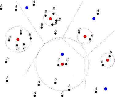
Figure 1: Illustration of the one2all construction proof with $\rho=1$. The data points $X$ are in black. The points in $M$ are colored red. We show the respective Voronoi partition and for each cluster, we show circles centered at the respective $m\in M$ (red) point with radius $\Delta_{m}$. The points in blue are a set $Q$. The points $x\in X$ are labeled $A$ if $d_{xQ}<2d_{xM}$ (and we apply Lemma 4.1). Otherwise, when there is a point $m$ such that $d_{xQ}>d_{xm}$, the point is labeled $B$ when $d_{mQ}\geq 2\Delta_{m}$ (Lemma 4.2) and is labeled $C$ otherwise (Lemma 4.3).

It remains to consider the complementary case where point $x$ is much closer to $M$ than to $Q$:

$$d_{xQ}\geq 2\rho d_{xM}\ .$$ (9)

We first introduce a useful definition: For a point $q\in M$, we denote by $\Delta_{q}$ the weighted median of the distances $d_{qy}$ for $y\in X_{q}$, weighted by $w_{y}$. The median $\Delta_{q}$ is a value that satisfies the following two conditions:

$$\sum_{x\in X_{q}\mid d_{xq}\leq\Delta_{q}}w_{x} \geq \frac{1}{2}w(X_{q})$$ (10)

$$\sum_{x\in X_{q}\mid d_{xq}\geq\Delta_{q}}w_{x} \geq \frac{1}{2}w(X_{m})\ .$$ (11)

It follows from (11) that for all $q\in M$,

$$V(M\mid X_{q},\boldsymbol{w}) = \sum_{x\in X_{q}}w_{x}d_{qx}\geq\sum_{x\in X_{q}\mid d_{xq}\geq\Delta_{q}}w_{x}d_{xq}$$

$$\geq\Delta_{q}\sum_{x\in X_{q}\mid d_{xq}\geq\Delta_{q}}w_{x}\geq\frac{1}{2}w(X_{m})\Delta_{q}\ .$$

Therefore,

$$V(M\mid X,\boldsymbol{w})=\sum_{q\in M}V(M\mid X_{q},\boldsymbol{w})\geq\frac{1}{2}\sum_{q\in M}w(X_{m})\Delta_{q}\ .$$ (12)

We now return to our proof for $x$ that satisfies (9). We will show that property (8) holds using the second term in the $\max$ operation in the definition (7). Specifically, let $m$ be the closest $M$ point to $x$. We will show that

$$\frac{d_{xQ}}{V(Q\mid X,\boldsymbol{w})}\leq 8\rho^{2}\alpha\frac{1}{w(X_{m})}\ .$$ (13)

We divide the proof to two subcases, in the two following Lemmas, each covering the complement of the other: When $d_{mQ}\geq 2\rho\Delta_{m}$ and when $d_{mQ}\leq 2\rho\Delta_{m}$.

Lemma 4.2

Let $x$ be such that

$$\exists m\in M,\ d_{mx}<\frac{1}{2\rho}d_{xQ}\text{ and }d_{mQ}\geq 2\rho\Delta_{m}\ .$$

Then

$$\frac{d_{xQ}}{V(Q\mid X,\boldsymbol{w})}\leq\frac{8\rho^{2}}{w(X_{m})}\ .$$

Proof

Let $q=\arg\min_{z\in Q}d_{mz}$ be the closest $Q$ point to $m$. From (relaxed) triangle inequality (6) and our assumptions:

$$d_{xQ}\leq d_{xq}\leq\rho(d_{mq}+d_{mx})=\rho(d_{mQ}+d_{mx})\leq\rho d_{mQ}+\frac{1}{2}d_{xQ}\ .$$

Rearranging, we get

$$d_{xQ}\leq 2\rho d_{mQ}\ .$$ (14)

Consider a point $y$ such that $d_{my}\leq\Delta_{m}$. Let $q^{\prime}=\arg\min_{z\in Q}d_{yz}$ be the closest $Q$ point to $y$. From relaxed triangle inequality we have $d_{mq^{\prime}}\leq\rho(d_{yq^{\prime}}+d_{ym})$ and therefore

$$d_{yQ} = d_{yq^{\prime}}\geq\frac{1}{\rho}d_{mq^{\prime}}-d_{ym}\geq\frac{1}{\rho}d_{mQ}-\Delta_{m}$$

$$\geq \frac{1}{\rho}d_{mQ}-\frac{1}{2\rho}d_{mQ}\geq\frac{1}{2\rho}d_{mQ}\ .$$

Thus, using the definition of $\Delta_{m}$ (10):

$$V(Q\mid X,\boldsymbol{w}) \geq \sum_{y\mid d_{yQ}\leq\Delta_{m}}w_{y}d_{yQ}\geq\frac{1}{2\rho}\sum_{y\mid d_{yQ}\leq\Delta_{m}}w_{y}d_{mQ}$$ (15)

$$\geq \frac{1}{2\rho}d_{mQ}\sum_{y\in X_{m}\mid d_{yQ}\leq\Delta_{m}}w_{y}$$

$$\geq \frac{1}{2\rho}d_{mQ}\frac{w(X_{m})}{2}=\frac{1}{4\rho}d_{mQ}w(X_{m})\ .$$

Combining (14) and (15) we obtain:

$$\frac{d_{xQ}}{V(Q\mid X,\boldsymbol{w})}\leq\frac{2\rho d_{mQ}}{\frac{1}{4\rho}w(X_{m})d_{mQ}}=8\rho^{2}\frac{1}{w(X_{m})}\ .$$

 

Lemma 4.3

Let a point $x$ be such that

$$\exists m\in M,\ d_{xm}<\frac{1}{2\rho}d_{xQ}\text{ and }d_{mQ}\leq 2\rho\Delta_{m}\ .$$

Then

$$\frac{d_{xQ}}{V(Q\mid X,\boldsymbol{w})}\leq 8\rho^{2}\alpha\frac{1}{w(X_{m})}\ .$$

Proof

Let $q=\arg\min_{z\in Q}d_{zm}$ be the closest $Q$ point to $m$. We have

$$d_{xQ}\leq d_{xq}\leq\rho(d_{xm}+d_{mq})\leq\frac{1}{2}d_{xQ}+\rho d_{mQ}\leq\frac{1}{2}d_{xQ}+2\rho^{2}\Delta_{m}$$

Therefore,

$$d_{xQ}\leq 4\rho^{2}\Delta_{m}\ .$$ (16)

Using (12) we obtain

$$V(Q\mid X,\boldsymbol{w}) \geq V(M\mid X,\boldsymbol{w})/\alpha\geq\frac{1}{2\alpha}\sum_{y\in M}w(X_{y})\Delta_{y}$$ (17)

$$\geq \frac{1}{2\alpha}w(X_{m})\Delta_{m}\ .$$

Combining (16) and (17) we obtain

$$\frac{d_{xQ}}{V(Q\mid X,\boldsymbol{w})}\leq\frac{4\rho^{2}\Delta_{m}}{\frac{1}{2\alpha}w(X_{m})\Delta_{m}}\leq 8\rho^{2}\alpha\frac{1}{w(X_{m})}\ .$$

 

$n$	$d$	$k$	guarantee $\epsilon$	adaptive $\frac{|S|}{n}$	worst-case $\frac{|S|}{n}$	$\times$ gain	est. err	$\frac{V(Q\mid X)}{V_{\text{ground-truth}}}$	$\frac{V(\{m_{0},\ldots,m_{k}\}\mid X)}{V_{\text{ground-truth}}}$	sweet-spot
Mixture of Gaussians data sets
$5\times 10^{5}$	$10$	$5$	$0.10$	$0.0500$	$1.00$	20.0	$0.008$	$1.07$	$2.50$	$2.3$
$5\times 10^{5}$	$10$	$5$	$0.20$	$0.0136$	$1.00$	73.3	$0.012$	$1.10$	$2.39$	$2.6$
$2.5\times 10^{6}$	$10$	$5$	$0.20$	$0.0025$	$1.00$	90.2	$0.0160$	$1.14$	$2.14$	$2.2$
$1\times 10^{7}$	$10$	$5$	$0.20$	$0.00066$	$1.00$	94.4	$0.018$	$1.12$	$2.07$	$2.6$
$2\times 10^{6}$	$10$	$20$	$0.10$	$0.04839$	$1.00$	20.7	$0.0018$	$1.14$	$2.27$	$9.1$
$2\times 10^{6}$	$10$	$20$	$0.20$	$0.012007$	$1.00$	83.2	$0.008$	$1.18$	$2.25$	$9.0$
$2\times 10^{6}$	$10$	$50$	$0.20$	$0.0298$	$1.00$	33.5	$0.0057$	$1.16$	$2.24$	$19.5$
$2\times 10^{6}$	$10$	$100$	$0.20$	$0.061918$	$1.00$	$16.2$	$0.0058$	$1.15$	$2.22$	$40.8$
$1\times 10^{6}$	$20$	$10$	$0.10$	$0.05293$	$1.00$	$18.9$	$0.0035$	$1.17$	$2.39$	$5.0$
$1\times 10^{6}$	$50$	$10$	$0.10$	$0.04726$	$1.00$	$21.2$	$0.0037$	$1.19$	$2.65$	$3.9$
$1\times 10^{6}$	$100$	$10$	$0.10$	$0.05287$	$1.00$	$18.9$	$0.0035$	$1.18$	$2.6$	$4.9$
MNIST data set
$6\times 10^{5}$	$784$	$10$	$0.20$	$0.0371$	$1.00$	26.9	$0.018$	$0.985$	$1.765$	$1.0$
Fashion data set
$6\times 10^{5}$	$784$	$10$	$0.20$	$0.05720$	$1.00$	17.5	$0.021$	$0.91$	$1.65$	$1.0$

Table 1: Clustering over a sample. The reported estimation error is $\sqrt{A[\left(\frac{V(Q\mid X)-V(Q\mid S)}{V(Q\mid X)}\right)^{2}]}$ .

Algorithm 1 Clustering cost oracle

// Preprocessing

Input: points $X$, weights $\boldsymbol{w}>\boldsymbol{0}$, iteration limit $\ell$, $C>0$, $\epsilon>0$

Output: Sample $S$ with weights $\boldsymbol{w}^{\prime}_{x}$ for $x\in S$

$s\leftarrow|X|$; $M\leftarrow\perp$

  // Initialization // Apply kmeans++ to $(X,\boldsymbol{w})$ and compute $\boldsymbol{p}$ foreach iteration $i\in[\ell]$ of kmeans++$(X,\boldsymbol{w})$ do

       $m_{i}\leftarrow$ new centroid selected ; $M\leftarrow M\cup\{m_{i}\}$ 

        // Centroids $v_{i}\leftarrow V(M\mid X,\boldsymbol{w})$

        // Clustering cost foreach $x\in X$ do // one2all probabilities (7)

            $p_{x}^{\prime}\leftarrow\min\{1,\max\{1,\frac{v_{i}}{C}\}\epsilon^{-2}\pi_{x}^{(M\mid X,\boldsymbol{w})}\}$

      if $|\boldsymbol{p}^{\prime}|_{1}<s$ then $\boldsymbol{p}\leftarrow\boldsymbol{p}^{\prime}$

       // best so far

// Compute sample from $\boldsymbol{p}$ $S\leftarrow$ include each $x\in X$ with probability $p_{x}$  

  // Poisson or varopt sample  foreach $x\in S$ do $w^{\prime}_{x}\leftarrow w_{x}/p_{x}$

 // inverse probability weights return $(S,\boldsymbol{w})$

  // weighted sample // Oracle Input: $Q$ such that $|Q|=k$; weighted sample $(S,w^{\prime}_{x})$ Output: Estimate of $V(Q\mid X,\boldsymbol{w})$ return $V(Q\mid S,\boldsymbol{w}^{\prime})$

Algorithm 2 Oracle with feedback for clustering cost

// Initialization

Input: Points $X$, weights $\boldsymbol{w}>\boldsymbol{0}$, $k$ , $\epsilon>0$

$\boldsymbol{p},C\leftarrow$ Probabilities $\boldsymbol{p}$ and cost $V(M_{2k})$ computed by Algorithm 1 with $\ell=2k$, $C=V(M_{2k})$ 
foreach $x\in X$ do $u_{x}\sim U[0,1]$

 // Randomization for sampling $S\leftarrow\{x\mid u_{x}\leq p_{x}\}$// Compute the sample  
foreach $x\in S$ do $w^{\prime}_{x}\leftarrow w_{x}/p_{x}$

 // weights for sampled points // Query processing with feedback Input: $Q$ such that $|Q|=k$ Output: Estimate of $V(Q\mid X,\boldsymbol{w})$ $\hat{V}\leftarrow V(Q\mid S,\boldsymbol{w}^{\prime})$

  // Sample-based estimate of $V(Q\mid X,\boldsymbol{w})$  if $\hat{V}>C$ then return $\hat{V}$

 // Return estimate and break // Increase sample size $V\leftarrow V(Q\mid X,\boldsymbol{w})$

  // Can also use estimate $\boldsymbol{p}\leftarrow(2C/V)*\boldsymbol{p}$ // increase sampling probabilities  
$C\leftarrow V/2$ // New cost threshold  
$S\leftarrow\{x\mid u_{x}\leq p_{x}\}$// Update the sample  
foreach $x\in S$ do $w^{\prime}_{x}\leftarrow w_{x}/p_{x}$

 // update weights   return $V$ 

5 Clustering cost oracle

A clustering cost oracle preprocesses the data $(X,\boldsymbol{w})$ and computes a compact structure from which clustering cost queries $Q$ can be efficiently approximated. Our basic oracle, Algorithm 1, inputs the data, iteration limit $\ell\geq 1$, $C>0$, and $\epsilon>0$. We will establish the following

Theorem 5.1

Algorithm 1 computes a weighted sample $(S,\boldsymbol{w}^{\prime})$. The inverse probability estimator (3) provides the pps quality guarantees of Theorem 2.1 and Corollary 2.1 for sets $Q$ with clustering cost at least $\alpha C$, where $\alpha\leq 1$.

Proof

The algorithm computes probabilities $\boldsymbol{\pi}:X$ that upper bound the base pps probabilities for all sets $Q$ of cost $V(Q)\geq C$. We perform $\ell$ iterations of kmeans++ on $(X,\boldsymbol{w})$. Each iteration $i$ computes a new centroid $m_{i}$ and we can also compute one2all base probabilities $\boldsymbol{\pi}^{(M_{i})}$, where $M_{i}=\{m_{1},\ldots,m_{i}\}$ for the set of the first $i$ centroids. Note that the computation of the one2all probabilities and the cost $V(M_{i}\mid X,\boldsymbol{w})$ does utilizes the distance computations and the assignment of points to the nearest centroid that is already performed by kmeans++. Each iteration $i$ yields candidate base probabilities $\boldsymbol{\pi}\leftarrow\max\{1,\frac{V(M_{i})}{C}\}*\boldsymbol{\pi}^{(M_{i})}$. From Corollary 3.1, each candidate base probabilities upper bound the base pps probabilities of all $Q$ with cost $V(Q)\geq C$. Finally, we retain, among the $\ell$ candidates, the one with minimum sample size $|\epsilon^{-2}*\boldsymbol{\pi}|_{1}$. This sweet-spot search replaces simply using $M_{\ell}$. Note that the size of the sample may increase with $i$, when $V(M_{i})$ drops slower than the increase in $i$. In our experiments we demonstrate the potential significant benefits of this adaptive optimization.

We proceed and compute a weighted sample $S$ (independent or varopt) according to probabilities $\boldsymbol{p}\leftarrow\epsilon^{-2}*\boldsymbol{\pi}$. For each $x\in S$ we associate a weight $w^{\prime}_{x}=w_{x}/p_{x}$. We process queries $Q$ by computing the clustering cost $V(Q\mid(S,\boldsymbol{w}^{\prime})$, which is equal to the inverse probability estimator (3) of the clustering cost of $Q$ over $(X,\boldsymbol{w})$.

Since $\boldsymbol{p}$ upper bound pps sampling probabilities for any $Q$ with $V(Q)\geq C$ and are within $V(Q)/C$ of the pps probabilities for any $Q$, the quality guarantees of Theorem 2.1 and Lemma 2.1 follow.  

Finally, note that the size of the oracle structure and the computation of each query are both linear in our sample size $|\boldsymbol{p}|_{1}$. The sample size we obtain using $M_{i}$ is (in expectation)

$$|\boldsymbol{p}|_{1}=\min_{i\in[\ell]}\max\{1,\frac{V(M_{i})}{C}\}\epsilon^{-2}*\boldsymbol{\pi}^{(M_{i})}\ .$$ (18)

A useful simple rough approximation for sample size that does not use the size parameter is

$$(8\rho^{2}|M|+2\rho)\frac{V(M_{i})}{C}\epsilon^{-2}=O(i\frac{V(M_{i})}{C})\propto iV(M_{i})\ .$$ (19)

5.1 Feedback oracle

We consider here constructing an oracle that provides quality guarantees for all $Q$ of size $k$.

Assume first that we are provided with $V^{*}$, which is the optimal clustering cost with $k$ clusters.

Lemma 5.1

Applying Algorithm 1 with $\ell=2k$ and $C=V^{*}$ provides us with a sample of expected size $O(k\epsilon^{-2})$ that provides the statistical guarantees of Theorem 2.1 (with $\alpha=1$).

Proof

From state-of-the-art bi-criteria bounds [29], we have that ${\textsf{E}}[V(M_{2k}\mid X,\boldsymbol{w})]/V^{*}]=O(1)$. The expected size of the sample, even with one2all applied to $M_{2k}$, is at most $2\frac{V(M_{2k})}{C}k\epsilon^{-2}8\rho^{2}=O(k\epsilon^{-2})$.

We comment that we can apply sweet-spot selection of $M_{i}$ even though $V(M_{2k})$ is not known before iteration $2k$, by using the rough approximation (19) instead of exact sample sizes. This allows for retaining one candidate $\boldsymbol{\pi}$ with the kmeans++ iterations.  

Note, however, that we do not know the optimal clustering cost $V^{*}$. One solution is to underestimate it: From the bi-criteria bounds we can compute large enough $\alpha$ (using Markov inequality) so that within the desired confidence value, $V(M_{2k}\mid X)/V^{*}\leq\alpha$. We can then apply the algorithm with $C=V(M_{2k})/\alpha$. But such a worst-case $\alpha$ is large (see Section 7) and forces a proportional increase in sample size, often needlessly so.

We instead propose a feedback oracle, detailed in Algorithm 2. We initialize with the basic oracle (Algorithm 5) with $\ell=2k$ and $C=V(M_{2k})$ to obtain probabilities $\boldsymbol{p}$. We draw a weighted sample $(S,\boldsymbol{w}^{\prime})$. The oracle processes a query $Q$ as follows. If $V(Q\mid S,\boldsymbol{w}^{\prime})\geq C$, it returns this estimate. Otherwise, we compute and return the exact cost $V(Q\mid X,\boldsymbol{w})$ and update the sample at the base of the oracle so that it supports queries with cost $\geq C=V(Q\mid X,\boldsymbol{w})/2$.

Note that each oracle call that results in an update halves (at least) the cost threshold $C$. Since we start with $C$ that is in expectation within a constant factor $\alpha$ from the optimal $k$ clustering cost, the expected total number of oracle calls that result in an update, is $\leq\log_{2}\alpha$. Moreover, the sample size is increased only in the face of evidence of a clustering with lower cost. So the final size uses $C\geq V^{*}/2$. For smoother estimates as the samples size increases, we coordinate the samples by using the same randomization $\boldsymbol{u}$. That way, new points are added to the sample when the size increases, but no points are removed.

Our feedback oracle provides the following statistical guarantees on estimate quality.

Theorem 5.2

A query $Q$ processed when $V(Q\mid X,\boldsymbol{w})\geq\alpha C$ ($\alpha\leq 1$) has the statistical guarantees as stated in Theorem 2.1. When $V(Q\mid X,\boldsymbol{w})=\alpha C$ for ($\alpha<1$), we either return an exact value or an overestimate with probability bounded by Corollary 2.1.

Algorithm 3 Clustering Wrapper

Input: points $X$, weights $\boldsymbol{w}>\boldsymbol{0}$, $\epsilon>0$, a clustering algorithm $\mathcal{A}$ that inputs a weighted set of points and returns $Q\in\mathcal{Q}$.

Output: Set $Q$ of $k$ centroids with statistical guarantees on quality over $X$ that match within $(1+\epsilon)$ those provided by $\mathcal{A}$

// Initialization

$c\leftarrow\infty$ // Apply kmeans++ to $(X,\boldsymbol{w})$

foreach iteration $i\in[2k]$ of kmeans++$(X,\boldsymbol{w})$ do

       $m_{i}\leftarrow$ next centroid 
$v_{i}\leftarrow V(\{m_{1},\ldots,m_{i}\}\mid X,\boldsymbol{w})$

        // Clustering cost if $iv_{i}<c$ then // sweet-spot one2all prob. (7)

            $\boldsymbol{\pi}\leftarrow\boldsymbol{\pi}^{(M\mid X,\boldsymbol{w})}$;  $V_{M}\leftarrow v_{i}$ ;  $c\leftarrow iv_{i}$

      

$r\leftarrow\frac{v_{M}}{v_{2k}}$

  // Initial sample size increase factor  $Q^{*}\leftarrow\{m_{1},\ldots,m_{k}\}$; $\overline{V}\leftarrow v_{k}$

  // Best so far and upper bound foreach $x\in X$ do $u_{x}\sim U[0,1]$

 // Randomization for sampling $S\leftarrow\{x\mid u_{x}\leq r\epsilon^{-2}\pi_{x}\}$ // Initial sample. $O(|S|)$ given preprocessed $\boldsymbol{\pi}$  
foreach $x\in S$ do $w^{\prime}_{x}\leftarrow w_{x}/\min\{1,r\pi_{x}\}$

 // weights for sampled points // Main Loop repeat

       // Cluster the sample $S$ $Q\leftarrow\mathcal{A}(S,\boldsymbol{w}^{\prime})$

        // Apply algorithm $\mathcal{A}$ to sample $V_{Q}\leftarrow V(Q\mid X,\boldsymbol{w})$

        // Exact or approx using a validation sample if $V_{Q}<\overline{V}$ then $\overline{V}\leftarrow V_{Q}$  $Q^{*}\leftarrow Q$

       if $V_{Q}\leq(1+\epsilon)V(Q\mid S,\boldsymbol{w}^{\prime})$ and $V_{Q}\geq V_{M}/r$ then

            break

      $r\leftarrow\max\{2,V_{Q}/V_{M}\}r$

        // Increase the sample size parameter repeat// Increase sample size until $Q$ is cleared

            $S\leftarrow\{x\mid u_{x}\leq r\epsilon^{-2}\pi_{x}\}$ // Add points to sample  
foreach $x\in S$ do $w^{\prime}_{x}\leftarrow w_{x}/\min\{1,r\pi_{x}\}$

             // weights for sampled points $r\leftarrow 2r$

      until $V(Q\mid S,\boldsymbol{w}^{\prime})>\min\{(1+\epsilon)\overline{V},(1-\epsilon)V_{Q}$}

      

until True

return $Q^{*}$

6 Clustering wrapper

The input to a clustering problem is a (weighted) set of points $(X,\boldsymbol{w})$ and $k>0$. The goal is to compute a set $Q$ of $k$ centroids aimed to minimize the clustering cost $V(Q\mid X,\boldsymbol{w})$.

We present a wrapper, Algorithm 3, which inputs a clustering problem, a clustering algorithm $\mathcal{A}$, and $\epsilon>0$, and returns a set of $Q$ of $k$ centroids. The wrapper computes weighted samples $(S,\boldsymbol{w}^{\prime})$ of the input points $(X,\boldsymbol{w})$ and applies $\mathcal{A}$ to $S$. It then performs some tests on the clustering $Q$ returned by $\mathcal{A}$, based on which, it either terminates and returns a clustering, or adaptively increases the sample size. The wrapper provides a statistical guarantee that the quality of the clustering $Q$ returned by $\mathcal{A}$ on the sample $(S,\boldsymbol{w}^{\prime})$ reflects, within $(1+\epsilon)$, its quality on the data.

The first part of the wrapper is similar to our clustering oracle Algorithm 1. We perform $2k$ iterations of kmeans++ tor $(X,\boldsymbol{w})$ to compute a list $\{m_{i}\}$ of centroids and respective clustering costs $v_{i}=V(\{m_{1},\ldots,m_{i}\}\mid X,\boldsymbol{w})$. While performing this computation, we identify a sweet-spot $M=\{m_{1},\ldots,m_{i}\}$ using the coarse estimate (19) of sample sizes and retain $\boldsymbol{\pi}:X$, which are the one2all base probabilities for $M$. Our wrapper separately maintains a size parameter $r$, that is initially set to $r=V_{i}/v_{2k}$. From Theorem 3.1, the probabilities $r*\boldsymbol{\pi}$ upper bound the base pps probabilities for all $Q$ with clustering cost $V(Q\mid(X,\boldsymbol{w}))\geq V_{M}/r$. Initially, $r*\boldsymbol{\pi}$ is set for cost above $v_{2k}$. We then selects a fixed randomization $\boldsymbol{u}$, that will allow for coordination of samples selected with different size parameters.

The main iteration computes a weighted sample $(S,\boldsymbol{w}^{\prime})$ selected with probabilities $\epsilon^{-2}r*\pi$. Our algorithm is applied to the sample $Q\leftarrow\mathcal{A}(S,\boldsymbol{w}^{\prime})$ to obtain a set $Q$ of $k$ centroids. We compute (or estimate from a validation sample) the clustering cost over the full dataset $V_{Q}=V(Q\mid x,\boldsymbol{w})$. If $V_{Q}$ is not lower than $V_{M}/r$ and is also not much higher than the sample clustering cost $V(Q\mid S,\boldsymbol{w}^{\prime})$, we break and return the best $Q$ we found so far. Otherwise, we increase the size parameter $r$, augment the sample accordingly, and iterate. The increase in the size parameter at least doubles it and is set so that (i) We have $V_{M}/r\leq\overline{V}$, where $\overline{V}$ is the smallest clustering cost encountered so far. (ii)  The set $Q$ that was underestimated by the sample has estimate that is high enough to clear it from $\overline{V}$ or to comprise an accurate estimate.

6.1 Analysis

We show that if our algorithm $\mathcal{A}$ provides a certain approximation ratio on the quality of the clustering, then this ratio would also hold (approximately, with high confidence) over the full data set. A similar argument applies to a bicriteria bound.

The wrapper works with an optimistic initial choice of $r$, but increases it adaptively as necessary. The basis of the correctness of our algorithm is that we are able to detect when our choice of $r$ is too low.

There are two separate issues that we tackle with adaptivity instead of with a pessimistic worst-case bound. The first is also addressed by our feedback oracle: For accurate estimates we need $V_{M}/r$ to be lower than $V^{*}=V(Q^{*}\mid X,\boldsymbol{w})$ (the optimal clustering cost over $X$), which we do not know. Initially, $V_{M}/r=v_{2k}$, which may be higher than $V^{*}$. We increase $r$ when we find a clustering $Q$ with $V(Q)<V_{M}/r$. The potential “bad” event is when the optimum clustering $Q^{*}$ has $V^{*}\ll V_{M}/r$ but is overestimated by a large amount in the sample resulting in the sample optimum $V^{*}_{S}$ is much larger than $V^{*}$. As a consequence, the clustering algorithm $\mathcal{A}$ applied to the sample can find $Q$, for which the estimate is correct, and has cost above $V_{m}/r$. The approximation ratio over the sample is $V(Q\mid S)/V^{*}_{S}$ which can be much better than the true (much weaker) approximation ratio $V(Q\mid S)/V^{*}$ over the full data.

This bad event happens when $V^{*}_{S}\gg V^{*}$. But note that in expectation, ${\textsf{E}}[V^{*}_{S}]\leq V^{*}$. Moreover, the probability of this bad event is bounded by $\exp(-\epsilon^{-2}/6)$ (see Theorem 2.1 and Corollary 2.1). We can make the probability of such bad event smaller by augmenting the wrapper as follows. When the wrapper is ready to return $Q$, we generate multiple samples of the same size and apply $\mathcal{A}$ to all these samples and take the best clustering generated. If we find a clustering with cost below $V_{m}/r$, we continue the algorithm. Otherwise, we return the best $Q$. The probability that all the repetitions are “bad” drops exponentially with the number of repetitions (samples) we use.

The second issue is inherent with optimization over samples. Suppose now that $r$ is such that $V^{*}\geq V_{M}/r$. The statistical guarantees provided by the sample are “ForEach,” which assure us that the cost is estimated well for a given $Q$. In particular, $V(Q^{*}\mid S,\boldsymbol{w}^{\prime})$ is well concentrated around $V^{*}$ (Theorem 2.1). This means that $V^{*}_{S}$, the optimal clustering cost over $S$, can only (essentially - up to concentration) be lower than $V^{*}$.

When we consider all $Q$ of size $k$, potentially an infinite or a very large number of them, it is possible that some $Q$ has clustering cost $V(Q\mid X,\boldsymbol{w})\gg V^{*}$ but is grossly underestimated in the sample, having sample-based cost $V(Q\mid S,\{w_{x}/p_{x}\})<V^{*}$. In this case, $V^{*}_{S}\ll V^{*}$ and our algorithm $\mathcal{A}$ that is applied to the sample will be fooled and can return such a $Q$. The worst-case approach to this issue is to use a union or a dimensionality bound that drastically increases sample size. We get around it using an adaptive optimization framework [12].

We can identify and handle this scenario, however, by testing $Q$ returned by the base algorithm to determine if our algorithm was “fooled” by the sample:

$$V(Q\mid X,\boldsymbol{w})\leq(1+\epsilon)V(Q\mid S,\{w_{x}/p_{x}\})\ .$$ (20)

by either computing the exact cost $V(Q\mid X,\boldsymbol{w})$ or by drawing another independent validation sample $S^{\prime}$, and using the estimate $V(Q\mid S,\{w_{x}/p_{x}\})$. When the test fails, we increase the sample size and repeat. In fact, we at least double the sample size parameter, but otherwise increase it at least to the point that $V(Q\mid S,\{w_{x}/p_{x}\})$ can no longer fool the algorithm. The only bad event possible here is that the sample optimum is much larger than $V(Q^{*})$. But as noted, when $V^{*}\geq V_{M}/r$ the probability of this for a particular sample is bounded by Theorem 2.1. Moreover, note that each increase of the sample size significantly strengthens the concentration of estimates for particular $Q$. Thus, the worst quality, over iterations, in which $Q^{*}$ is estimated in the sample is dominated by the first iteration with $V(Q^{*})\geq V_{M}/r$. Therefore, the approximation ratio over the sample is at least (up to the statistical concentration of the estimates of $Q^{*}$) the ratio over the full data.

6.2 Computation

The computation performed is dominated by two components. The first is the $2k$ iterations of kmeans++ on the data, which are dominated by $2k|X|$ pairwise distance computations. These is the only component that must be performed over the original data. The second is the application of $\mathcal{A}$ to the sample. When $\mathcal{A}$ is (super)linear, it is dominated by the largest sample we use.

Note that correctness does not depend on using $2k$ iterations. We can apply one2all to any set $M$. The only catch is that we may end up using a very large value of $r$ and a larger sample size. An added optimization, which is not in the pseudocode, is to perform the kmeans++ iterations more sparingly. Balancing the size of the sample (the final parameter $r$ and its product with $M$) and the computation cost of additional iterations over the full data.

7 Experiments

We performed illustrative experiments for Euclidean $k$-means clustering on both synthetic and real-world data sets. We implemented our wrapper Algorithm 3 in numpy with the following base clustering algorithm $\mathcal{A}$: We use $5$ applications of kmeans++ and take the set of $k$ centroids that has the smallest clustering cost. This set is used as an initialization to 20 iterations of Lloyd’s algorithm. The use of kmeans++ to initialize Lloyd’s algorithm is a prevalent method in practice.

Synthetic data:

We generated synthetic data sets by drawing $n$ points $X\subset R^{d}$ from a mixture of $k$ Gaussians. The means of the Gaussians are arranged to lie in a line with equal distances. The standard deviations of the Gaussians were drawn from a range equal to the distance to the closest mean. As a reference, we use the means of the Gaussians as the ground truth centroids.

MNIST and Fashion MNIST datasets:

We use the MNIST data set of images of handwritten digits [23] and the Fashion data set of images of clothing items [30]. Both data sets contain $n=6\times 10^{5}$ images coded as $d=784$ dimensional vectors. There are $k=10$ natural classes that correspond to the 10 digits or 10 types of clothing items. Our reference ground-truth centroids were taken as the mean of each class.

Worst-case bounds:

We also report, for comparison, sizes based on state-of-the-art coresets constructions that provide the same statistical guarantees. The coreset sizes are determined using worst-case upper bounds. When constant factors are not specified, we underestimate them. The constructions can be viewed as having two components. The first is an upper bound on the size of a coreset that provides an ForEach guarantee. For our purposes, we would also need a constructive way to obtain such a coreset. The second is an upper bound on the increase factor that is needed to obtain an ForAll guarantee. We make here gross underestimates of worst-case coreset sizes. The best bound on an ForEach coreset size is slightly underestimated by $8\rho^{2}k\epsilon^{-2}=32k\epsilon^{-2}$. For an actual construction, we can use kmeans++ and the tightest worst-case bounds on the bicriteria approximation quality it provides. The state of the art [29] is that with $\beta k$ centroids we are (in expectation) within a factor of $8(1+\varphi/(\beta-1))$ of the optimal clustering cost (for Euclidean metric), where $\varphi\approx 1.618$ is the golden ratio. There are no concentration results, and Markov inequality is used to obtain confidence bounds: There is 50% probability of being below twice this expectation, which is $16(1+\varphi/(\beta-1))$.

The sample size depends both on the number of centroids we use and on the approximation quality: We need to minimize the product of $\beta$ and the approximation factor. The expression $\beta(1+\varphi/(\beta-1))$ for $\beta>1$ is minimized at $\beta\approx 1.53$ and the factor is $\approx 6.1$. So we obtain an increase factor on sample size that is at least $6\times 16=96$.

Combining this all, we get an underestimate of $96*32*k\epsilon^{-2}\approx 3000k\epsilon^{-2}$ for that component. We then consider the bound on the increase factor. The state of the art bounds [6], based on union bound and dimensionality arguments, are $O(\min(n,d/\epsilon))$ for Euclidean and $O(\log k\log n)$ for general metric spaces. The hidden constant factors are not specified and we underestimate them here to be equal to $1$. Combining, we underestimate the best worst-case bound on coreset size by

$$\min\{n,3000k\epsilon^{-2}\min\{\log k\log n,\min(n,d/\epsilon)\}\ .$$

Adaptive bounds:

Table 1 reports the results of our experiments. The first four columns report the basic parameters of each data set: The number of points $n$, clusters $k$, dimension $d$, and the specified value of $\epsilon$ for the desired statistical guarantee. The middle columns report the final sample size $|S|$ used by the algorithm as a fraction of $n$, an underestimate on the corresponding coreset size from state of the art worst-case bounds, and the gain factor in sample size by using our adaptive algorithm instead of a worst-case bound. We can observe significant benefit that increases with the size of the data sets. On the MNIST data, the worst-case approach provides no data reduction.

The third set of columns reports the accuracy of the sample-based estimate of the cost of the final clustering $Q$. We can see that the error is very small (much smaller than $\epsilon$). We also report the quality of the final clustering $Q$ and the quality of the clusters obtained by applying kmeans++ to $X$, relative to the cost of the “ground truth” centroids. We can see that the cost of the final clustering is very close (in the case of MNIST, is lower) than the “ground truth” cost. We also observe significant improvement over the cost of the kmeans++ centroids used for initialization.

The last column reports the number of kmeans++ iterations on the full data set that was eventually used (the sweet spot value). This sweet spot optimizes for the overhead per sample size. This means that in effect fewer than $k$ kmeans++ iterations over the full data were used.

Finally, we take a closer look at the benefit of the number of iterations of kmeans++ that are performed on the full data set and used as input to one2all. Figure 2 shows properties for the sequence of centroids $\{m_{i}\}$ returned by the kmeans++ algorithms on the mnist, fashion-mnist, and one of the mixture synthetics datasets with $k=20$ natural clusters. The first is the clustering cost of each prefix, divided by the cost of the ground truth clustering. We can see that on our synthetic data with spread out clusters there is significant cost reduction with the first few iterations whereas with the two natural data sets, the cost of the first (random) centroids is within a factor 3 of the ground-truth cost with 10 centroids. The second plot shows the sample size “overhead factor” when we use one2all on a prefix $\{m_{1},\ldots,m_{i}\}$ of the kmeans++ centroids to obtain ForEach guarantees for $Q$ with clustering costs that are at least the ground-truth cost. To do so, we apply one2all to the set with $\alpha=V(\{m_{1},\ldots,m_{i}\}\mid X)/V_{\text{ground-truth}}$. The resulting overhead is proportional to

$$\alpha i=\frac{V(\{m_{1},\ldots,m_{i}\}\mid X)}{V_{\text{ground-truth}}}i\ .$$

We can see that with our two natural data sets, the sweet spot is obtained with the first centroid. Moreover, most of the benefit is already obtained after 5 centroids.

For the task of providing an efficient clustering costs oracle, we would like to also optimize the final sample size. We can see that the sweet-spot choice of the number of centroids provides significant benefit (order of magnitude reduction on the natural data set) compared to the worst-case choice (of using $\approx 1.5k$ centroids).

For clustering, the figure provides indication for the benefit of additional optimization which incorporates the cost versus benefit of additional kmeans++ iterations that are performed on the full data set $X$. As mentioned, we can adaptively perform additional iterations as to balance its cost with the computation and accuracy we have on a sample that is large enough to meet ForEach for $k$-clusters: Even on data sets where the sweet-spot required more iterations, a prohibitive cost of performing them on the full data set may justify working with a larger sample.

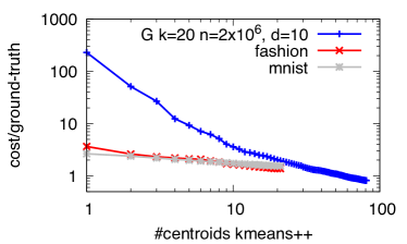
Figure 2: Left: Clustering cost (divided by ground-truth clustering cost) for first $i$ centroids found by kmeans++ on full data set (averaged over 10 iterations). Right: Sample size overhead factor when applying one2all to $\{m_{1},\ldots,m_{i}\}$ to provide ForEach guarantees for clustering costs that are at least the ground truth cost.

8 Conclusion

We consider here clustering of a large set of points $X$ in a (relaxed) metric space. We present a clustering cost oracle, which estimates the clustering cost of an input set of centroids from a small set of sampled points, and a clustering wrapper that inputs a base clustering algorithm which it applies to small sets of sampled points. At the heart of our design are our one2all base probabilities that are asigned to the points $X$. These probabilities are defined with respect to a set $M$ of centroids but yet, a sample of size $O(\alpha^{-1}|M|)$ (for $\alpha\geq 1$) allows us to estimate the clustering cost of any set of centroids $Q$ with cost that is at least $V(M)/\alpha$.

Our clustering cost oracle and wrapper work with weighted samples taken using the one2all probabilities for a set $M$ of centroids computing using the kmeans++ algorithm. Our oracle adaptively increase the sample size (effectively increasing “$\alpha$”) when encountering $Q$ with cost lower than $V(M)/\alpha$. Our wrapper increases the sample size when the clustering returned by the base algorithm has sample cost that is either below $V(M)/\alpha$ or does not match the cost over the full data (invoking a method of adaptive optimization over samples [12]).

A salient feature of our oracle and clustering wrapper methods is that we start with an optimistic small sample and increase it adaptively only in the face of hard evidence that a larger sample is indeed necessary for meeting the specified statistical guarantees on quality. Previous constructions use worst-case size summary structures that can be much larger. We demonstrate experimentally the very large potential gain, of orders of magnitude in sample sizes, when using our adaptive versus worst-case methods.

Beyond estimation and optimization of clustering cost, the set of distances of each $Q$ to the one2all sample $S$ is essentially a sketch of the full (weighted) distance vector of $Q$ to $X$ [14]. Sketches of different sets $Q$ allow us to estimate relations between the respective full vectors, such as distance norms, weighted Jaccard similarity, quantile aggregates, and more, which can be useful building blocks in other applications.

Moreover, Euclidean $k$-means clustering is a constrained rank-$k$ approximation problem, and this connection facilitated interesting feedback between techniques designed for low-rank approximation and for clustering [15]. We thus hope that our methods and the general method of optimization over multi-objective sample [12] might lead to further progress on other low-rank approximation problems.

References

- [1] P. K. Agarwal, S. Har-Peled, and K. R. Varadarajan. Geometric approximation via coresets. In Combinatorial and computational geometry, MSRI. University Press, 2005.
- [2] A. Aggarwal, A. Deshpande, and R. Kannan. Adaptive sampling for k-means clustering. In RANDOM, 2009.
- [3] D. Aloise, A. Deshpande, P. Hansen, and P. Popat. NP-hardness of Euclidean sum-of-squares clustering. Mach. Learn., 75(2), 2009.
- [4] D. Arthur and S. Vassilvitskii. K-means++: The advantages of careful seeding. In SODA, 2007.
- [5] P. Awasthi, M. Charikar, R. Krishnaswamy, and A. K. Sinop. The hardness of approximation of Euclidean k-means. In SoCG, 2015.
- [6] V. Braverman, D. Feldman, and H. Lang. New frameworks for offline and streaming coreset constructions. CoRR, abs/1612.00889, 2016.
- [7] K. R. W. Brewer, L. J. Early, and S. F. Joyce. Selecting several samples from a single population. Australian Journal of Statistics, 14(3):231–239, 1972.
- [8] M. T. Chao. A general purpose unequal probability sampling plan. Biometrika, 69(3):653–656, 1982.
- [9] S. Chechik, E. Cohen, and H. Kaplan. Average distance queries through weighted samples in graphs and metric spaces: High scalability with tight statistical guarantees. In RANDOM. ACM, 2015.
- [10] K. Chen. On coresets for k-median and k-means clustering in metric and Euclidean spaces and their applications. SIAM J. Comput., 39(3), 2009.
- [11] E. Cohen. Size-estimation framework with applications to transitive closure and reachability. J. Comput. System Sci., 55:441–453, 1997.
- [12] E. Cohen. Multi-objective weighted sampling. In HotWeb. IEEE, 2015. full version: http://arxiv.org/abs/1509.07445.
- [13] E. Cohen, N. Duffield, C. Lund, M. Thorup, and H. Kaplan. Efficient stream sampling for variance-optimal estimation of subset sums. SIAM J. Comput., 40(5), 2011.
- [14] E. Cohen, H. Kaplan, and S. Sen. Coordinated weighted sampling for estimating aggregates over multiple weight assignments. VLDB, 2(1–2), 2009. full: http://arxiv.org/abs/0906.4560.
- [15] M. B. Cohen, S. Elder, C. Musco, C. Musco, and M. Persu. Dimensionality reduction for k-means clustering and low rank approximation. In STOC. ACM, 2015.
- [16] D. Feldman and M. Langberg. A unified framework for approximating and clustering data. In STOC. ACM, 2011.
- [17] D. Feldman, M. Schmidt, and C. Sohler. Turning big data into tiny data: Constant-size coresets for k-means, PCA and projective clustering. In SODA. ACM-SIAM, 2013.
- [18] M. H. Hansen and W. N. Hurwitz. On the theory of sampling from finite populations. Ann. Math. Statist., 14(4), 1943.
- [19] S. Har-Peled and S. Mazumdar. On coresets for k-means and k-median clustering. In STOC. ACM, 2004.
- [20] D. G. Horvitz and D. J. Thompson. A generalization of sampling without replacement from a finite universe. Journal of the American Statistical Association, 47(260):663–685, 1952.
- [21] T. Kanungo, D. M. Mount, N. S. Netanyahu, C. D. Piatko, R. Silverman, and A. Y. Wu. A local search approximation algorithm for k-means clustering. Computational Geometry, 28(2), 2004.
- [22] L. Kish and A. Scott. Retaining units after changing strata and probabilities. Journal of the American Statistical Association, 66(335):pp. 461–470, 1971.
- [23] Y. LeCun and C. Cortes. MNIST handwritten digit database. 2010.
- [24] S. Lloyd. Least squares quantization in PCM. IEEE Trans. Inf. Theor., 1982.
- [25] R. R. Mettu and C. G. Plaxton. Optimal time bounds for approximate clustering. Mach. Learn., 56(1-3), 2004.
- [26] P. J. Saavedra. Fixed sample size pps approximations with a permanent random number. In Proc. of the Section on Survey Research Methods, pages 697–700, Alexandria, VA, 1995. American Statistical Association.
- [27] C-E. Särndal, B. Swensson, and J. Wretman. Model Assisted Survey Sampling. Springer, 1992.
- [28] Y. Tillé. Sampling Algorithms. Springer-Verlag, New York, 2006.
- [29] D. Wei. A constant-factor bi-criteria approximation guarantee for k-means++. In NIPS, 2016.
- [30] H. Xiao, K. Rasul, and R. Vollgraf. Fashion-mnist: a novel image dataset for benchmarking machine learning algorithms. CoRR, abs/1708.07747, 2017.