Effective description of correlations for states obtained from conformal field theory

Abstract

We study states of one- and two-dimensional spin systems that are constructed as correlators within the conformal field theory of a massless, free boson. In one dimension, these are good variational wave functions for XXZ spin chains and they are similar to lattice Laughlin states in two dimensions. We show that their $zz$ correlations are determined by a modification of the original free-boson theory. An expansion to quadratic order leads to a solvable, effective theory for the correlations in these states. Compared to the massless boson, there is an additional term in this effective theory that explains the behavior of the correlations: a polynomial decay in one dimension and at the edge of a two-dimensional system and an exponential decay in the bulk of a two-dimensional system. We test the validity of our approximation by comparing it to Monte Carlo computations.

I Introduction

Conformal field theory (CFT) in $1+1$ dimensions is characterized by the absence of an intrinsic energy scale and has applications in various fields including string theory, statistical mechanics, and condensed matter physics. In the latter case, CFT arises as the continuous, field theoretical description of low-energy degrees of freedom of critical lattice models in one spatial dimension (1D). Traditionally, this connection is established by explicitly taking the continuum limit of a lattice Hamiltonian, potentially integrating out high-energy modes through renormalization, and mapping operators of the original problem to continuous fields.

In the past decades, another approach in applying CFT to problems in condensed matter physics was established. In this case, CFT is used to construct variational wave functions for interacting many-body systems, both in 1D and in two spatial dimensions (2D). This idea reaches back to Laughlin’s description of the fractional quantum Hall (FQH) effectLaughlin (1983) and the realization that the Laughlin wave function and its generalizations are correlators in a CFTMoore and Read (1991). Such a construction was then also established for systems on a latticeCirac and Sierra (2010), where the corresponding states can be understood as generalizations of matrix product states to the case of an infinite bond dimensionCirac and Sierra (2010). Within this framework, many interesting states and model systems were obtained including 1D critical and FQH lattice statesNielsen et al. (2012); Tu et al. (2014); Glasser et al. (2015, 2016); Hackenbroich and Tu (2017).

The fact that variational wave functions constructed from CFT provide good descriptions of FQH states may seem surprising: In the bulk, a FQH system is gapped and has exponentially decaying correlations whereas a CFT is gapless and CFT correlators decay polynomially. This raises the question of how the CFT influences the properties of corresponding states.

In the past years, it was realized that the entanglement entropy and spectra carry signatures of the underlying CFT: In 1D, the entanglement entropy of a CFT exhibits a logarithmic violation of the area law and this characteristic behavior was observed in corresponding lattice systemsVidal et al. (2003); Calabrese and Cardy (2004). Furthermore, the energy levels of CFTs were found in the entanglement spectra of 1DLäuchli (2013) and of FQH states Li and Haldane (2008); Sterdyniak et al. (2012); Dubail et al. (2012a); Rodríguez et al. (2012). In addition to its entanglement properties, the CFT nature of a state also affects its correlations. While both CFT correlators and those of a critical 1D state decay polynomially, the relation is more intricate for 2D states, which decay polynomially only at the edge of a 2D system. Assuming that their bulk correlations decay exponentially, it was shown in Ref. Dubail et al., 2012b that edge correlations of a FQH state follow from those of the underlying CFT. So far, our knowledge concerning bulk correlations relies on numerical computations, mostly of Monte Carlo typeCaillol et al. (1982); Nielsen et al. (2012).

The purpose of this paper is to clarify the relation between the correlations in a state and the CFT it is constructed from. We express these correlations as expectation values in a field theory that is a modification of the original CFT. This explains the different types of correlations, in particular those in the bulk of a 2D system as emerging from a mass-like perturbation of the CFT.

The idea of treating the effect of a FQH wave function as a perturbation of the underlying CFT was introduced in a general context in Refs. Read, 2009; Dubail et al., 2012b. The screening property, i.e. exponentially decaying bulk correlations, was assumed in Ref. Dubail et al., 2012b. Here, we provide analytical evidence for screening for a specific type of FQH states: By an expansion of the exact representation of the correlations, we derive an effective action that has a mass-like term in the bulk of the system, thus giving rise to exponentially decaying bulk correlations.

Concretely, we study a set of states that are constructed from the CFT of a free, massless boson. These are defined for a system of spin-$\frac{1}{2}$ degrees of freedom on a lattice. In addition to the lattice position, they have one parameter corresponding to the scaling dimension of CFT primary fields. In 1D, these states are good descriptions of ground states of the XXZ spin chain in the half-filled sector Cirac and Sierra (2010) and they resemble lattice Laughlin states in 2D Nielsen et al. (2012). For the $zz$ spin correlations, we derive an exact path integral representation and then truncate it to quadratic order to obtain an effective, free theory. In contrast to the free-boson CFT, the action of this effective theory has a mass-like term, which corresponds to the scaling dimension of the primary fields that define our states. Within the approximation of a free field theory, the correlations on lattices can be computed efficiently for large system sizes. Taking a continuum limit, we furthermore obtain analytical results for the approximate $zz$ correlations. Our calculations provide evidence for a power-law decay in 1D and at the edge of a 2D system and an exponential decay in the bulk of a 2D system. This behavior is a consequence of the mass-like term in the effective theory.

We test the validity of our approximation in 1D and 2D by comparing the results to Monte Carlo computations. Our analysis shows that the approximation is better for smaller scaling dimensions. Furthermore, it is applicable for a larger range of scaling dimensions in the case of a 2D system compared to a 1D system.

This paper is structured as follows. Sec. II describes the construction of states from the free-boson CFT and Sec. III derives an effective description of their $zz$ correlations. In Sec. IV, we describe our solution to the effective theory within a continuum limit and on lattices. The results of our approximation are compared to the exact correlations in Sec. V.

II Spin states from conformal fields

We consider a free, massless bosonic field $\phi(z,\bar{z})$ in one spatial dimension with the Euclidean action

$$S_{0}[\phi] =\frac{1}{4\pi}\int dzd\bar{z}\partial_{z}\phi(z,\bar{z})\partial_{\bar{z}}\phi(z,\bar{z}),$$ (1)

where $z$ and $\bar{z}$ are coordinates in the complex plane. The field $\phi(z,\bar{z})$ decomposes into a chiral part $\phi(z)$ and an anti-chiral part $\bar{\phi}(\bar{z})$ according to $\phi(z,\bar{z})=\phi(z)+\bar{\phi}(\bar{z})$. The chiral and anti-chiral sectors of the free-boson theory define CFTs with central charges $c=1$ and $\bar{c}=1$, respectively. The vertex operators

$$:e^{i\sqrt{\alpha}s\phi(z)}:$$ (2)

are chiral primary fields with a scaling dimension of $\alpha/2$.Di Francesco et al. (1997) Here, $\alpha$ is a positive real parameter, $s\in\{-1,1\}$, and the colons denote normal ordering. We consider $N$ vertex operators at distinct positions $z_{j}$ in the complex plane:

$$\mathcal{V}^{\alpha}_{s_{j}}(z_{j})=\chi_{j,s_{j}}:e^{i\sqrt{\alpha}s_{j}\phi(z_{j})}:,$$ (3)

where $\chi_{j,s_{j}}$ are $2N$ phase factors ($|\chi_{j,s_{j}}|=1$) that we leave unspecified since the correlations computed in this work are independent of the choice of $\chi_{j,s_{j}}$. The CFT correlator of these operators defines the spin states $\psi_{\alpha}$ through

$$|\psi_{\alpha}\rangle =\sum_{s_{1},\dots,s_{N}}\psi_{\alpha}(s_{1},\dots,s_{N})|s_{1},\dots,s_{N}\rangle,$$ (4)

$$\psi_{\alpha}(s_{1},\dots,s_{N}) =\langle\mathcal{V}^{\alpha}_{s_{1}}(z_{1})\dots\mathcal{V}^{\alpha}_{s_{N}}(z_{N})\rangle.$$ (5)

Here, $s_{j}\in\{-1,1\}$, $|s_{1},\dots,s_{N}\rangle$ is the tensor product of eigenstates of the spin-$z$ operator $t^{z}_{j}$ at position $j$ in the spin-$1/2$ representation $\left(t^{z}_{j}|s_{j}\rangle=\frac{s_{j}}{2}|s_{j}\rangle\right)$, and $\langle\dots\rangle$ denotes the radially ordered vacuum expectation value in the free-boson CFT. Evaluating the CFT correlator leads to Di Francesco et al. (1997)

$$\psi_{\alpha}(s_{1},\dots,s_{N})=\delta_{\mathbf{s}}\prod_{j=1}^{N}\chi_{j,s_{j}}\prod_{i<j}^{N}(z_{i}-z_{j})^{\alpha s_{i}s_{j}},$$ (6)

where $\delta_{\mathbf{s}}=1$ if $\sum_{j=1}^{N}s_{j}=0$ and $\delta_{\mathbf{s}}=0$ otherwise. Due to the charge neutrality condition $\sum_{j=1}^{N}s_{j}=0$, the states $\psi_{\alpha}$ have a vanishing $z$ component of the total spin.

For a 2D system, $\psi_{\alpha}$ is similar to the Laughlin lattice state with $\nu=\frac{1}{4\alpha}$ particles per fluxNielsen et al. (2012). In particular, $\alpha=\frac{1}{4}$ corresponds to an integer quantum Hall state with one particle per flux and $\alpha=\frac{1}{2}$ to the Kalmeyer-Laughlin FQH state with $1/2$ particle per flux. When $4\alpha$ is not an integer, the states $\psi_{\alpha}$ can be thought of as generalizations of FQH lattice states.

III Effective description of correlations

In this section, we derive an effective description of the $zz$ correlations in the states $\psi_{\alpha}$ in terms of a free field theory. The $zz$ correlations between lattice points $i$ and $j$ are defined as

$$\langle\sigma^{z}_{i}\sigma^{z}_{j}\rangle =4\frac{\langle\psi_{\alpha}|t^{z}_{i}t^{z}_{j}|\psi_{\alpha}\rangle}{\langle\psi_{\alpha}|\psi_{\alpha}\rangle}$$ (7)

$$=\frac{\sum_{s_{1},\dots,s_{N}}s_{i}s_{j}|\psi_{\alpha}(s_{1},\dots,s_{N})|^{2}}{\sum_{s_{1},\dots,s_{N}}|\psi_{\alpha}(s_{1},\dots,s_{N})|^{2}}.$$ (8)

In the following, it is assumed that the sites $i$ and $j$ are distinct since the correlator for $i=j$ can be evaluated trivially, $\langle\sigma^{z}_{i}\sigma^{z}_{i}\rangle=1$. We first derive an exact representation of $\langle\sigma^{z}_{i}\sigma^{z}_{j}\rangle$, which we then truncate to an effective, quadratic theory.

III.1 Exact field theory representation of correlations

Let us first consider the normalization $\langle\psi_{\alpha}|\psi_{\alpha}\rangle$ in Eq. (7). Using the form of the wave function of Eq. (6), $\langle\sigma^{z}_{i}\sigma^{z}_{j}\rangle$ can be written as a vacuum expectation value of vertex operators in the complete free-boson theory (chiral and anti-chiral):

$$\langle\psi_{\alpha}|\psi_{\alpha}\rangle$$

$$\quad=\sum_{s_{1},\dots,s_{N}}|\psi_{\alpha}(s_{1},\dots,s_{N})|^{2}$$ (9)

$$\quad=\sum_{s_{1},\dots,s_{N}}\delta_{\mathbf{s}}\prod_{i<j}|z_{i}-z_{j}|^{2\alpha s_{i}s_{j}}$$ (10)

$$\quad=\sum_{s_{1},\dots,s_{N}}\langle:e^{i\sqrt{\alpha}s_{1}\phi(z_{1},\bar{z}_{1})}:\dots:e^{i\sqrt{\alpha}s_{N}\phi(z_{N},\bar{z}_{N})}:\rangle,$$ (11)

where $\delta_{\mathbf{s}}\prod_{i<j}|z_{i}-z_{j}|^{2\alpha s_{i}s_{j}}$ was written as the correlation function of $N$ vertex operators $:e^{i\sqrt{\alpha}s_{j}\phi(z_{j},\bar{z}_{j})}:$. Note that the condition imposed by $\delta_{\mathbf{s}}$ is implicitly contained in Eq. (11) since the correlator of vertex operators vanishes unless $s_{1}+\dots+s_{N}=0$.

Carrying out each of the sums over $s_{j}$,

$$\sum_{s_{j}\in\{-1,1\}}:e^{i\sqrt{\alpha}s_{j}\phi(z_{j},\bar{z}_{j})}:=2:\cos\left(\sqrt{\alpha}\phi(z_{j},\bar{z}_{j})\right):,$$ (12)

we obtain

$$\langle\psi_{\alpha}|\psi_{\alpha}\rangle =2^{N}\langle\prod_{k=1}^{N}:\cos\left(\sqrt{\alpha}\phi(z_{k},\bar{z}_{k})\right):\rangle.$$ (13)

For the numerator in Eq. (7), we additionally use

$$\sum_{s_{j}\in\{-1,1\}}s_{j}:e^{i\sqrt{\alpha}s_{j}\phi(z_{j},\bar{z}_{j})}: =2i:\sin\left(\sqrt{\alpha}\phi(z_{j},\bar{z}_{j})\right):$$ (14)

and obtain

$$4\langle\psi_{\alpha}|t^{z}_{i}t^{z}_{j}|\psi_{\alpha}\rangle$$

$$=\sum_{s_{1},\dots,s_{N}}s_{i}s_{j}\langle:e^{i\sqrt{\alpha}s_{1}\phi(z_{1},\bar{z}_{1})}:\dots:e^{i\sqrt{\alpha}s_{N}\phi(z_{N},\bar{z}_{N})}:\rangle$$ (15)

$$=-2^{N}\langle:\sin\left(\sqrt{\alpha}\phi(z_{i},\bar{z}_{i})\right)::\sin\left(\sqrt{\alpha}\phi(z_{j},\bar{z}_{j})\right):\times$$

$$\quad\phantom{-2^{N}}\times\prod_{k(\neq i,j)}^{N}:\cos\left(\sqrt{\alpha}\phi(z_{k},\bar{z}_{k})\right):\rangle,$$ (16)

where $k(\neq i,j)$ denotes all indices $k$ that are distinct from $i$ and $j$. Therefore, the expression for the $zz$ correlations becomes

$$\langle\sigma^{z}_{i}\sigma^{z}_{j}\rangle =-\frac{\langle:\sin\left(\sqrt{\alpha}\phi(z_{i},\bar{z}_{i})\right)::\sin\left(\sqrt{\alpha}\phi(z_{j},\bar{z}_{j})\right):\prod_{k(\neq i,j)}^{N}:\cos\left(\sqrt{\alpha}\phi(z_{k},\bar{z}_{k})\right):\rangle}{\langle\prod_{k=1}^{N}:\cos\left(\sqrt{\alpha}\phi(z_{k},\bar{z}_{k})\right):\rangle\rangle}.$$ (17)

As we show in Appendix  A, one can drop the normal ordering in this expression since this changes the numerator and denominator by the same constant factor. Thus, the path integral representation of Eq. (17) is given by

$$\langle\sigma^{z}_{i}\sigma^{z}_{j}\rangle =-\frac{\int\mathcal{D}\phi\tan\left(\sqrt{\alpha}\phi(z_{i},\bar{z}_{i})\right)\tan\left(\sqrt{\alpha}\phi(z_{j},\bar{z}_{j})\right)\cos\left(\sqrt{\alpha}\phi(z_{1},\bar{z}_{1})\right)\dots\cos\left(\sqrt{\alpha}\phi(z_{N},\bar{z}_{N})\right)e^{-S_{0}[\phi]}}{\int\mathcal{D}\phi\cos\left(\sqrt{\alpha}\phi(z_{1},\bar{z}_{1})\right)\dots\cos\left(\sqrt{\alpha}\phi(z_{N},\bar{z}_{N})\right)e^{-S_{0}[\phi]}}.$$ (18)

This expression determines the exact $zz$ correlations in $\psi_{\alpha}$.

III.2 Effective theory for correlations

The starting point of our approximation is to expand the path integral representation of Eq. (18) to quadratic order in $\phi(z,\bar{z})$ around $0$. This is motivated by the following observation: For large $N$, the contribution of the integrand in Eq. (18) is only significant for field configurations that have $\cos(\sqrt{\alpha}\phi(z_{j},\bar{z}_{j}))\approx\pm 1$ at all positions $z_{j}$. At the same time, the massless, free-boson action $S_{0}[\phi]$ suppresses field configurations that change rapidly through the derivative term. Therefore, the fields dominating the path integral are those for which $\sqrt{\alpha}\phi(z,\bar{z})$ is near the same extremum of cosine for all positions $z$. Since $S_{0}[\phi]$ is invariant under a constant shift of the field value, $\phi(z,\bar{z})\to\phi(z,\bar{z})+\text{const.}$, we can focus on the case $\phi(z,\bar{z})\approx 0$. The expansion around the extremum of the cosine function is analogous to Kosterlitz and Thouless’s treatment of the XY model Kosterlitz and Thouless (1973); Kosterlitz (1974). We are, however, not taking into account terms that would correspond to vortex configurations in the XY model.

Hence, we expand $\cos(\sqrt{\alpha}\phi(z,\bar{z}))\sim e^{-\frac{\alpha}{2}\phi(z,\bar{z})^{2}}$ and $\tan(\sqrt{\alpha}\phi(z,\bar{z}))\sim\sqrt{\alpha}\phi(z,\bar{z})$ in Eq. (18) and obtain

$$\langle\sigma^{z}_{i}\sigma^{z}_{j}\rangle \approx-\alpha\frac{\int\mathcal{D}\phi\;\phi(z_{i},\bar{z}_{i})\phi(z_{j},\bar{z}_{j})e^{-S_{\alpha}[\phi]}}{\int\mathcal{D}\phi e^{-S_{\alpha}[\phi]}},$$ (19)

where

$$S_{\alpha}[\phi] =\frac{1}{4\pi}\int dzd\bar{z}\partial_{z}\phi(z,\bar{z})\partial_{\bar{z}}\phi(z,\bar{z})+\frac{\alpha}{2}\sum_{j=1}^{N}\phi(z_{j},\bar{z}_{j})^{2}.$$ (20)

The quadratic action $S_{\alpha}$ provides an effective theory that approximately describes the $zz$ correlations in the state $\psi_{\alpha}$. Compared to the action of the free, massless boson, it has an additional mass-like term at the positions of the lattice.

IV Solution schemes for 1D and 2D lattices

In the following, we describe two solution schemes to the quadratic action $S_{\alpha}$ of Eq. (20), which determines the approximate $zz$ correlations in the state $\psi_{\alpha}$. The first scheme consists of taking a continuum limit of the lattice. This further simplification allows us to derive analytical results for the approximate $zz$ correlations. The second scheme keeps the structure of the lattice and is solved numerically.

IV.1 Continuum approximation

We apply an additional approximation to the action $S_{\alpha}$ by writing the sum over the positions $z_{j}$ as an integral. We replace the sum over positions $\sum_{j=1}^{N}\phi(z_{j},\bar{z}_{j})^{2}$ in Eq. (20) by a term proportional to the integral $\int_{D}dzd\bar{z}\phi(z,\bar{z})^{2}$, where $D$ is the region in the complex plane in which the spins are located. The precise form of this replacement depends on the given system and is provided in Appendix C.1, where we also compute the approximate $zz$ correlations of Eq. (19) using the Green’s function formalism. We considered the systems illustrated in Fig. 1: a 1D system (infinite line and circle), a 2D system without a boundary (sphere), and a 2D system with a boundary (half plane and half-infinite cylinder). Our results in the continuum limit are summarized in Table 1.

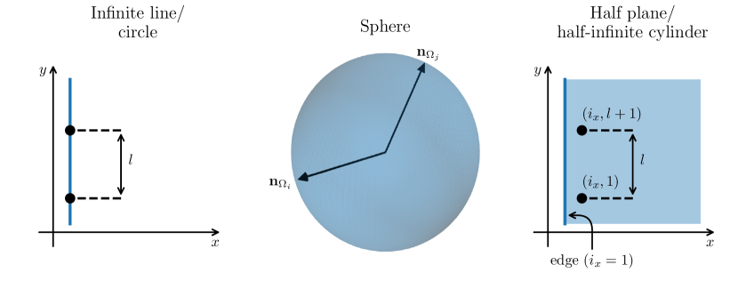
Figure 1: (Color online) Systems for the computation of the $zz$ correlations in the continuum approximation. The spins are located in the blue regions. In the case of the circle and the half-infinite cylinder, periodic boundary conditions are imposed along the $y$ direction. The two points shown in each of the panels are the sites for which the $zz$ correlations were computed.

Note that the continuum approximation predicts a power law decay of the long-range correlations in a 1D and at the edge of a 2D system with the power being $-2$ independent of $\alpha$. In the bulk of a 2D system, we find an exponential decay of the correlations at large distances.

Table 1: Approximation of the $zz$ correlations in $\psi_{\alpha}$ in the continuum approximation, cf. Fig. 1 for an illustration of the different systems. $\Phi(z,s,a)=\sum_{m=0}^{\infty}z^{m}/(a+m)^{s}$ denotes the Lerch transcendent function, $\mathrm{Si}$ and $\mathrm{Ci}$ are the sine and cosine integral functions, respectively. The position on the sphere $\mathbf{n}_{\Omega_{i}}\in S^{2}$ is defined in Eq. (28).

System	$zz$ correlations	Large-distance limit ($l\gg 1$)
Infinite line	$\langle\sigma^{z}_{l+1}\sigma^{z}_{1}\rangle\approx 2\alpha\left[\cos\left(r\right)\mathrm{Ci}\left(r\right)+\sin\left(r\right)\left(\mathrm{Si}\left(r\right)-\frac{\pi}{2}\right)\right]$,	$-\frac{1}{2\pi^{2}\alpha}\frac{1}{l^{2}}$
($l=0,1,2,\dots$)	with $r=2\pi\alpha l$
Circle	$\langle\sigma^{z}_{l+1}\sigma^{z}_{1}\rangle\approx\frac{1}{N}-2\alpha\mathrm{Re}\left[\Phi\left(e^{2\pi i\frac{l}{N}},1,N\alpha\right)\right]$
($l=0,1,\dots,N-1$)
Sphere $\left(\mathbf{n}_{\Omega_{i}},\mathbf{n}_{\Omega_{j}}\in S^{2}\right)$	$\langle\sigma^{z}_{i}\sigma^{z}_{j}\rangle\approx-\alpha\int_{0}^{\infty}dq\frac{2\cos\left(\sqrt{N\alpha-\frac{1}{4}}q\right)}{\sqrt{2\cosh(q)-2+|\mathbf{n}_{\Omega_{i}}-\mathbf{n}_{\Omega_{j}}|^{2}}}$
Half-plane	$\langle\sigma^{z}_{i_{x},l+1}\sigma^{z}_{i_{x},1}\rangle\approx\int_{-\infty}^{\infty}\frac{dq}{2\pi}e^{-iql}g(q)$,	edge ($i_{x}=1$): $-\frac{1}{\pi l^{2}}$
$\begin{aligned} (i_{x}&=1,2,\dots;\\ l&=0,1,2,\dots)\end{aligned}$	with $g(q)=-\frac{2\pi\alpha}{\sqrt{4\pi\alpha+q^{2}}}\left[1+\frac{4\pi\alpha e^{-2\left(i_{x}-1\right)\sqrt{4\pi\alpha+q^{2}}}}{\left(\left|q\right|+\sqrt{4\pi\alpha+q^{2}}\right)^{2}}\right]$	bulk ($i_{x}\to\infty$): $-\pi^{\frac{1}{4}}\alpha^{\frac{3}{4}}\frac{e^{-2\sqrt{\pi\alpha}l}}{\sqrt{l}}$
Half-infinite cylinder	$\langle\sigma^{z}_{i_{x},l+1}\sigma^{z}_{i_{x},1}\rangle\approx\frac{1}{N_{y}}\sum_{m=-\infty}^{\infty}e^{-\frac{2\pi iml}{N_{y}}}g(\frac{2\pi m}{N_{y}})$,
$\begin{aligned} (i_{x}&=1,2,\dots;\\ l&=0,1,\dots,N_{y}-1)\end{aligned}$	with $g(q)$ as for the half-plane

IV.2 Discrete approximation

The continuum approximation of the previous subsection does not take into account the lattice structure of the states $\psi_{\alpha}$. In order to test this simplification and to obtain a better approximation of the exact $zz$ correlations, we now discuss an approximation scheme that keeps the lattice. Specifically, we discuss three types of lattices: a uniform lattice on a circle, an approximately uniform lattice on the sphere, and a square lattice on the cylinder. Thus, we can study both a 1D system and 2D systems with and without edges.

In the discrete case, we do not work with the path integral representation of the approximate $zz$ correlations of Eq. (20) since it contains short-distance divergences at the lattice positions $z_{j}$. Taking the continuum limit as done above is one way to remove these divergences. In the discrete case, we choose to work with normal ordered fields and thus avoid divergences. This corresponds to taking the normal ordered expression of Eq. (17) as the starting point of the approximation instead of the path integral representation of Eq. (18). The approximation of the $zz$ correlation then becomes

$$\langle\sigma^{z}_{i}\sigma^{z}_{j}\rangle \approx-\alpha\frac{\langle:\phi(z_{i},\bar{z}_{i})e^{-\frac{\alpha}{2}\phi(z_{i},\bar{z}_{i})^{2}}::\phi(z_{j},\bar{z}_{j})e^{-\frac{\alpha}{2}\phi(z_{j},\bar{z}_{j})^{2}}:\prod_{k(\neq i,j)}^{N}:e^{-\frac{\alpha}{2}\phi(z_{k},\bar{z}_{k})^{2}}:\rangle}{\langle\prod_{k=1}^{N}:e^{-\frac{\alpha}{2}\phi(z_{k},\bar{z}_{k})^{2}}:\rangle}.$$ (21)

In Appendix C.2, we compute this expression and find

$$\langle\sigma^{z}_{i}\sigma^{z}_{j}\rangle \approx\Gamma_{i,j},$$ (22)

where

$$\Gamma_{i,j} =\left[T_{r}\left(T_{r}^{t}MT_{r}+\mathbf{e}_{r}\mathbf{e}_{r}^{t}\right)^{-1}T_{r}^{t}-\mathbb{I}\right]_{i,j},$$ (23)

$r\in\{1,\dots,N\}$ is an arbitrary index, $M$ and $T_{r}$ are the $N\times N$ with entries

$$M_{m,n} =\delta_{m,n}-2\alpha\ln\left(d_{m,n}+\delta_{m,n}\right),$$ (24)

$$\left(T_{r}\right)_{m,n} =\delta_{m,n}-\delta_{m,r},$$ (25)

$\mathbf{e}_{r}$ is the $r$th unit vector, and $\mathbb{I}$ is the identity matrix. The $N\times N$ matrix $d_{i,j}$ contains the distances between sites $i$ and $j$. It is given by $d_{i,j}=|z_{i}-z_{j}|$ for positions in the complex plane. We note that the matrix $\Gamma$ is independent of the choice of $r$.

IV.2.1 Definition of lattices

We now define the lattices on the circle, sphere, and the cylinder and discuss how to ensure that the approximation retains the symmetries of the lattice.

The positions of a uniform lattice on the circle are given by

$$z_{j} =e^{\frac{2\pi i}{N}j},\text{ with }j\in\{1,\dots,N\}.$$ (26)

In the case of the sphere, we would like to work with a lattice that has an approximately uniform distribution of points on the sphere embedded in three-dimensional space. Following Ref. Nielsen et al., 2012, we generate such a lattice by minimizing the objective function

$$\sum_{i<j}^{N}\frac{1}{|\mathbf{n}_{\Omega_{i}}-\mathbf{n}_{\Omega_{j}}|^{2}},$$ (27)

where $\mathbf{n}_{\Omega_{j}}$ is given in terms of the polar angle $\theta_{j}$ and the azimuthal angle $\varphi_{j}$ as

$$\mathbf{n}_{\Omega_{j}}=\left(\begin{matrix}\sin(\theta_{j})\cos(\varphi_{j})\\ \sin(\theta_{j})\sin(\varphi_{j})\\ \cos(\theta_{j})\end{matrix}\right).$$ (28)

When computing the exact $zz$ correlations, the positions on the sphere can be mapped to the complex plane using the stereographic projection $z_{j}=\tan\left(\theta_{j}/2\right)e^{-i\varphi_{j}}$. For the approximate $zz$ correlations, however, it is better not to do this projection but to work directly on the sphere. The reason is that the differences in the complex plane, $|z_{m}-z_{n}|=|e^{-i\varphi_{m}}\tan(\theta_{m}/2)-e^{-i\varphi_{n}}\tan(\theta_{n}/2)|$, are not invariant under general rotations of the sphere. Note that this is not a problem for the exact $zz$ correlations since

$$\langle\sigma^{z}_{i}\sigma^{z}_{j}\rangle =\frac{\sum_{s_{1},\dots,s_{N}}s_{i}s_{j}\delta_{\mathbf{s}}\prod_{m<n}|z_{m}-z_{n}|^{2\alpha s_{m}s_{n}}}{\sum_{s_{1},\dots,s_{N}}\delta_{\mathbf{s}}\prod_{m<n}|z_{m}-z_{n}|^{2\alpha s_{m}s_{n}}}$$

$$=\frac{\sum_{s_{1},\dots,s_{N}}s_{i}s_{j}\delta_{\mathbf{s}}\prod_{m<n}|\mathbf{n}_{\Omega_{m}}-\mathbf{n}_{\Omega_{n}}|^{2\alpha s_{m}s_{n}}}{\sum_{s_{1},\dots,s_{N}}\delta_{\mathbf{s}}\prod_{m<n}|\mathbf{n}_{\Omega_{m}}-\mathbf{n}_{\Omega_{n}}|^{2\alpha s_{m}s_{n}}},$$ (29)

where $|\mathbf{n}_{\Omega_{m}}-\mathbf{n}_{\Omega_{n}}|$ is invariant under sphere rotations. [Eq. (29) follows from $|\mathbf{n}_{\Omega_{m}}-\mathbf{n}_{\Omega_{n}}|=2\cos(\theta_{m}/2)\cos(\theta_{n}/2)|z_{m}-z_{n}|$ and $s_{1}+\dots+s_{N}=0$.] As we show in Appendix (B.1), the replacement of $|z_{m}-z_{n}|$ by $|\mathbf{n}_{\Omega_{m}}-\mathbf{n}_{\Omega_{n}}|$ corresponds to working directly on the sphere instead of the complex plane. Doing our approximation for the free-boson field $\phi(\theta,\varphi)$ instead of $\phi(z,\bar{z})$ thus leads us to an approximation that keeps the rotation invariance on the sphere. It is given by the expressions following Eq. (22) with $d_{m,n}=|\mathbf{n}_{\Omega_{m}}-\mathbf{n}_{\Omega_{n}}|$.

The positions on the cylinder with $N_{x}$ sites in the open direction and $N_{y}$ sites in the periodical direction are defined as

$$w_{j} =\frac{2\pi}{N_{y}}(j_{x}+ij_{y}),$$ (30)

where $j_{x}\in\{1,\dots,N_{x}\}$ and $j_{y}\in\{1,\dots,N_{y}\}$ are the $x$ and $y$ components of the index $j$, respectively [$j=(j_{x}-1)N_{y}+j_{y}$]. The positions $w_{j_{x},j_{y}+N_{y}}$ and $w_{j_{x},j_{y}}$ are identified to impose periodicity in the $y$ direction. Usually, the coordinates $w_{j}$ on the cylinder are projected onto the complex plane through $z_{j}=e^{w_{j}}$. As for the stereographic projection in the case of the sphere, this mapping is, however, not a symmetry of the approximate $zz$ correlations. Even though $|z_{i}-z_{j}|$ does not change under rotations of the cylinder, it distorts distances. As we show in Appendix B.2, working with coordinates $w_{j}$ instead of $z_{j}=e^{w_{j}}$ corresponds to the replacement $|z_{i}-z_{j}|\to d_{i,j}$ with

$$d_{i,j} =\left|2\sinh\left(\frac{1}{2}(w_{i}-w_{j})\right)\right|.$$ (31)

Our approximation on the cylinder is thus obtained by expanding in the field $\phi(w,\bar{w})$ instead of $\phi(z,\bar{z})$. The resulting approximation of $\langle\sigma^{z}_{i}\sigma^{z}_{j}\rangle$ is given by using $d_{i,j}$ of Eq. (31) in the expressions following Eq. (22).

IV.2.2 Choice of the lattice scale

The exact $zz$ correlations are invariant under rescaling transformations of the lattice due to the conformal symmetry of the correlator of Eq. (5). These change the distances according to

$$d_{m,n}\to\lambda d_{m,n},$$ (32)

where $\lambda>0$. The quadratic, discrete approximation of $\langle\sigma^{z}_{i}\sigma^{z}_{j}\rangle$ is, however, not invariant under such rescalings since the matrix $M$ of Eq. (24) varies under a change of the lattice scale $\lambda$. Thus, different choices of $\lambda$ lead to different values of the approximation and we need a criterion to uniquely determine the value of $\lambda$. We note that this problem does not occur in the continuum approximation since the replacement of the sum over lattice positions by an integral restores scale invariance as shown in Appendix C.1. In order to fix $\lambda$ in the discrete case, we computed the subleading term of the expansion for the $zz$ correlations in Appendix C.2:

$$\langle\sigma^{z}_{i}\sigma^{z}_{j}\rangle\approx\Gamma_{i,j}-\Gamma_{i,j}(\Gamma_{i,i}+\Gamma_{j,j}).$$ (33)

For two given indices $i$ and $j$, we define the optimal scale $\lambda$ by requiring that it minimizes the subleading term of the expansion, i.e. it is a minimum of

$$|\Gamma_{i,i}+\Gamma_{j,j}|.$$ (34)

Instead of choosing different scales for the different values of $i$ and $j$, we also considered the following simpler approach: For a given set of positions and value of $\alpha$, we determine a single optimal scale $\lambda$ by minimizing the expression

$$\sqrt{\sum_{j=1}^{N}\Gamma_{j,j}^{2}}.$$ (35)

In addition to minimizing expression (34) or (35), we require that $\lambda$ is chosen such that eigenvalues of the matrix $T_{r}^{t}MT_{r}+\mathbf{e}_{r}\mathbf{e}_{r}^{t}$ appearing in Eq. (23) are all positive. This condition ensures the convergence of an $N$-dimensional Gaussian integral, cf. the derivation in Appendix C.2. As our numerical calculations show, these requirements uniquely determine the value of $\lambda$.

We did computations with multiple optimizations, i.e. minimizing expression (34), and a single optimization of expression (35). We found that doing multiple optimizations does not result in a substantial improvement of our results. Therefore, the data shown in the following correspond to a single optimization for a given lattice and value of $\alpha$.

V Quality of approximation for different systems

In this Section, we test the validity of our approximation by comparing the obtained $zz$ correlations to their actual value. Our aim in doing this analysis is to test whether the simple picture of the effective, quadratic theory is accurate. In two special cases, the actual $zz$ correlations can be computed exactly, namely for $\alpha=\frac{1}{4}$, where $\psi_{\alpha}$ is the wave function of $\frac{N}{2}$ free fermions Nielsen et al. (2012), and for $\alpha=\frac{1}{2}$ on the circle, where the exact correlations are known analytically Nielsen et al. (2011); Stéphan and Pollmann (2017). For all other cases, we used a Metropolis Monte Carlo method to obtain estimates of the exact $zz$ correlations in $\psi_{\alpha}$. The approximation data in the following plots was computed using the discrete scheme described in Sec. IV.2. We restrict ourselves to the four values of $\alpha=0.125,0.25,0.375$, and $\alpha=0.5$ here. Plots for additional values of $\alpha$ as well as for the continuum approximation can be found in the Supplementary Materialsup .

V.1 One-dimensional system

We first consider a 1D system. In this case, we can compare our results to bosonization studies of the XXZ model

$$H_{\mathrm{XXZ}} =\sum_{j=1}^{N}\left(t^{x}_{j}t^{x}_{j+1}+t^{y}_{j}t^{y}_{j+1}+\Delta t^{z}_{j}t^{z}_{j+1}\right),$$ (36)

where $t^{a}_{N+1}=t^{a}_{1}$ for periodic boundary conditions. This model is in a critical phase for anisotropies $-1<\Delta\leq 1$. The wave function $\psi_{\alpha}$ was used previously Cirac and Sierra (2010) as a variational ansatz for $H_{\mathrm{XXZ}}$ in the half-filled sector ($t^{z}_{1}+\dots+t^{z}_{N}=0$). More precisely, the positions $z_{j}$ were taken to be uniformly distributed on a circle and $\alpha$ was determined for a given value of $\Delta$ such that the variational energy in $\psi_{\alpha}$ is minimal. In the critical phase, the optimal value of $\alpha$ approximately satisfies $\Delta=-\cos(2\pi\alpha)$ and the overlap between the exact ground state $\psi_{0}$ and the optimal $\psi_{\alpha}$ is large Cirac and Sierra (2010). Using the relation $\Delta=-\cos(2\pi\alpha)$, the results for the long-range $zz$ correlations obtained using bosonization Luther and Peschel (1975); Lukyanov (1999) are given by

$$\frac{\langle\psi_{0}|\sigma^{z}_{l+1}\sigma^{z}_{1}|\psi_{0}\rangle}{\langle\psi_{0}|\psi_{0}\rangle} \sim-\frac{1}{2\pi^{2}\alpha}\frac{1}{l^{2}}+A\frac{(-1)^{l}}{l^{\frac{1}{2\alpha}}},$$ (37)

where $A$ is the $\alpha$-dependent amplitude that was determined in Ref. Lukyanov, 1999. In the bosonization formalism, the local Pauli matrix $\sigma^{z}_{i}$ has two contributions: A smooth term proportional to the U(1) current $\partial_{y}\phi(y)$ and a second, rapidly varying term proportional to $\cos(\pi y+\sqrt{2\pi}\phi(y))$.Cabra and Pujol (2004) The decay of correlations with a power of $-2$ originates from the correlator of two U(1) currents, while the rapidly varying term in the representation of $\sigma^{z}_{i}$ causes the staggered contribution to Eq. (37).

For small values of $\alpha$, the first term in Eq. (37) is dominant. Our analytical results for the long-range correlations in an infinite 1D system of Table 1 correctly reproduce this term. As $\alpha$ approaches $\frac{1}{4}$, however, the second, alternating term in Eq. (37) becomes relevant and eventually dominates for $\alpha>\frac{1}{4}$. In this regime, the state develops quasi-long-range antiferromagnetic order. This behavior is not captured by the results of our continuum approximation. In contrast to bosonization, our representation of the $zz$ correlations neglects rapid changes with position by assuming that the boson field is close to the same extremum of cosine at all positions, cf. Sec. III.2. Furthermore, our approximation assumes that $\sqrt{\alpha}\phi(z,\bar{z})$ is small and therefore we do not expect to obtain the second term in Eq. (37), which is relevant for large $\alpha$.

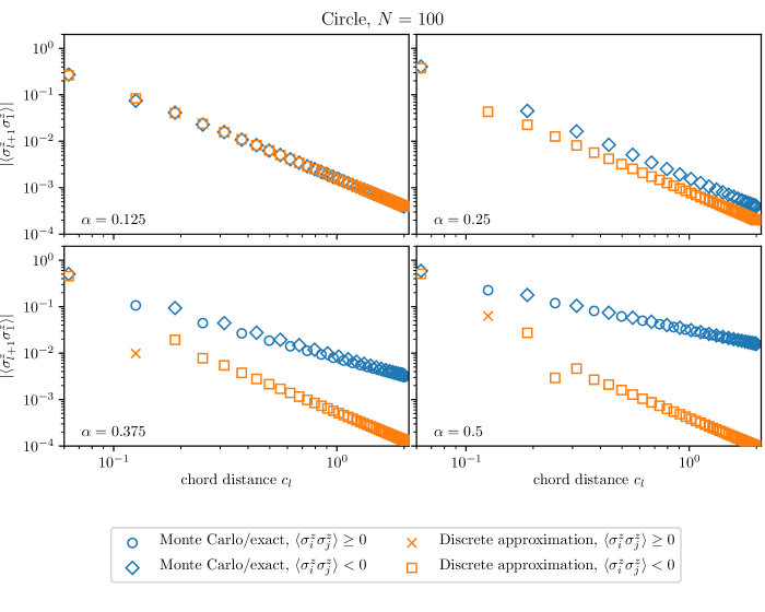
Figure 2: (Color online) $zz$ correlations in $\psi_{\alpha}$ for $N=100$ spins uniformly distributed on the circle. The data shown in blue are Monte Carlo estimates ($\alpha=0.125$ and $\alpha=0.375$) or exact ($\alpha=0.25$ and $\alpha=0.5$). The Monte Carlo errors are of the order of $10^{-6}$ and are thus not visible. The horizontal axes show the chord distance $c_{l}=|2\sin(\pi l/N)|$. At $\alpha=0.25$, every second value of the actual correlator (blue symbols) is zero within numerical error and thus not visible.

Let us now discuss our numerical results for the discrete approximation. These are shown for $N=100$ spins uniformly distributed on the circle in Fig. 2. At large distances, we observe a polynomial decay in the correlations. (Both axes in Fig. 2 are scaled logarithmically.) We find good agreement between the Monte Carlo estimate of the exact correlator and the approximation for $\alpha=0.125$. The results differ substantially from the exact correlator for $\alpha\geq 0.25$ and the deviation grows with $\alpha$. In particular, the oscillating behavior of $\langle\sigma^{z}_{l+1}\sigma^{z}_{1}\rangle$ for $\alpha>0.25$ is not reproduced by our approximation.

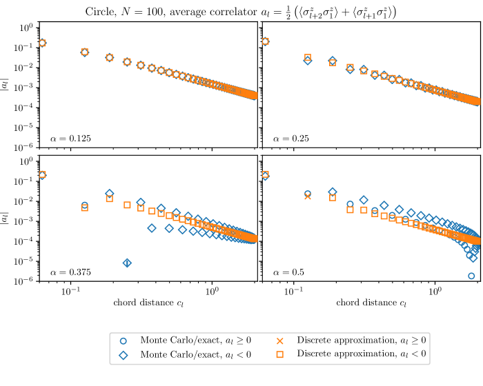
Figure 3: (Color online) Average $a_{l}=\frac{1}{2}(\langle\sigma^{z}_{l+2}\sigma^{z}_{1}\rangle+\langle\sigma^{z}_{l+1}\sigma^{z}_{1}\rangle)$ between in the $zz$ correlations in $\psi_{\alpha}$ at distances $l$ and $l+1$ for $N=100$ spins on the circle. The blue symbols correspond to numerically exact data for $\alpha=0.25$ and $\alpha=0.5$ and to Monte Carlo estimates for $\alpha=0.125$ and $\alpha=0.375$. The horizontal axes show the chord distance $c_{l}=|2\sin(\pi l/N)|$.

To further emphasize that the approximation captures the smooth part of the correlator but not the alternating one, we consider the average $a_{l}=\frac{1}{2}(\langle\sigma^{z}_{l+2}\sigma^{z}_{1}\rangle+\langle\sigma^{z}_{l+1}\sigma^{z}_{1}\rangle)$ between the correlator at distances $l+1$ and $l$. This combination suppresses the oscillating term at large distances:

$$\frac{1}{2}\left(\frac{\langle\psi_{0}|\sigma^{z}_{l+2}\sigma^{z}_{1}|\psi_{0}\rangle}{\langle\psi_{0}|\psi_{0}\rangle}+\frac{\langle\psi_{0}|\sigma^{z}_{l+1}\sigma^{z}_{1}|\psi_{0}\rangle}{\langle\psi_{0}|\psi_{0}\rangle}\right)$$

$$\quad\sim-\frac{1}{2\pi^{2}\alpha l^{2}}+A\frac{(-1)^{l}}{4\alpha l^{1+\frac{1}{2\alpha}}}$$ (38)

for the correlator obtained through bosonization. The average $a_{l}$ is plotted in Fig. 3 for the actual $zz$ correlations in $\psi_{\alpha}$ and those obtained within the discrete approximation. Indeed, the agreement for $a_{l}$ is better also for larger values of $\alpha$. [The value of $\alpha=\frac{1}{2}$ is special in the sense that $a_{l}$ still oscillates as a function of the distance. The reason is that both terms in Eq. (V.1) for $\alpha=\frac{1}{2}$ decay with the same power and the amplitude of the oscillating term dominates. While this oscillation is absent in the approximation, the power of the decay of $a_{l}$ agrees with the actual one.]

In summary, both the comparison to bosonization and to the exact correlator lead to the conclusion that our approximation is only valid for small values of $\alpha$ in 1D.

V.2 Two-dimensional system without a boundary (sphere)

We next discuss the case of a 2D system without a boundary. The results of the discrete approximation are compared to the exact $zz$ correlations in Fig. 4 for $N=100$ spins on the sphere. The distribution of sites on the sphere was chosen to be approximately uniform. In Fig. 4, the vertical axis is scaled logarithmically, while the horizontal axis is linear.

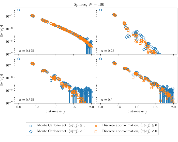
Figure 4: (Color online) $zz$ correlations in $\psi_{\alpha}$ for $N=100$ spins with an approximately uniform distribution on the sphere. The blue data points are Monte Carlo estimates ($\alpha=0.125,0.375,0.5$) or exact ($\alpha=0.25$). The horizontal axes show the distance $d_{1,j}=\left|\mathbf{n}_{\Omega_{1}}-\mathbf{n}_{\Omega_{j}}\right|$, cf. Eq. (28) for the definition of $\mathbf{n}_{\Omega_{j}}$.

Both the approximate correlations and the actual ones decay exponentially. Furthermore, a similar transition in the behavior of the $zz$ correlations appears at $\alpha=\frac{1}{4}$ as in 1D: For $\alpha\leq\frac{1}{4}$, the correlations between distinct sites are negative whereas for $\alpha>\frac{1}{4}$ they change sign as a function of the distance. As in 1D, we find the best agreement for the smallest value of $\alpha$ and large deviations at the transition point $\alpha=\frac{1}{4}$. However, in contrast to the 1D case, the approximation captures the qualitative behavior of the correlations for larger values of $\alpha$. In particular, we observe that the sign changes are reproduced correctly.

A reason for the better performance of the approximation in 2D could be as follows: Due to the cosine factors in Eq. (18), we assumed field configurations around $0$ mainly contribute to the path integral. In the case of a 1D system, however, these cosine factors only depend on the field configuration along a 1D path and therefore they do not restrict contributions to the path integral as strongly as for a 2D system. Furthermore, the oscillations in the actual correlations are much stronger in 1D, where they decay polynomially, than in 2D, where the decay is exponential and there is no quasi-long-range antiferromagnetic order.

V.3 Two-dimensional system with a boundary (cylinder)

Let us now consider a 2D system with an edge. Our results for the edge correlations of a cylinder of size $N_{x}=14$ and $N_{y}=160$ are shown in Fig. 5. (The large number of spins $N_{y}=160$ is chosen so that we can study the long-range decay of edge correlations.)

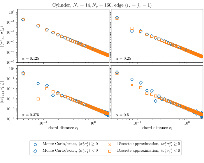
Figure 5: (Color online) $zz$ correlations in $\psi_{\alpha}$ on the edge of a cylinder with $N_{x}=14$ sites in the open direction and $N_{y}=160$ sites in the periodical direction. The shown correlations are those along the $y$ direction. The blue data points are Monte Carlo estimates ($\alpha=0.125,0.375,0.5$) or exact ($\alpha=0.25$). The horizontal axes show the chord distance $c_{l}=|2\sin(\pi l/N_{y})|$.

For $\alpha=0.125$, we observe a good agreement at all length scales. As $\alpha$ becomes larger, the approximation deviates from the exact result at short distances but follows the decay at larger ones to good accuracy. The plots in Fig 5 are logarithmically scaled on both axes and therefore show an algebraic decay of long-range correlations with a power of $-2$ as predicted by our continuum approximation (cf. Table 1). This behavior corresponds to the decay of a current-current correlator of a U(1) theory at the edge.

Our results for the correlator in the bulk of the cylinder are shown in Fig. 6.

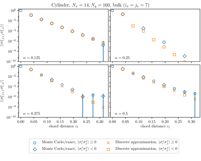
Figure 6: (Color online) $zz$ correlations in $\psi_{\alpha}$ in the bulk of a cylinder with $N_{x}=14$ sites in the open direction and $N_{y}=160$ sites in the periodical direction. The shown correlations are those along the $y$ direction. The blue data points are Monte Carlo estimates ($\alpha=0.125,0.375,0.5$) or exact ($\alpha=0.25$). The horizontal axes show the chord distance $c_{l}=|2\sin(\pi l/N_{y})|$. We only plot the data at short distances since the correlations decay exponentially and good Monte Carlo estimates cannot be obtained at larger distances. At $\alpha=0.25$, every second data point of the actual correlator (blue symbols) assumes a value below the lower boundary of the plot and is thus not visible.

The agreement between the approximate and the actual correlator is similar to that on the sphere: The approximation is best for $\alpha=0.125$, fails to describe the transition at $\alpha=0.25$, and is qualitatively right for $\alpha>0.25$. The approximate correlations and the actual ones decay exponentially. (The horizontal axes in Fig. 6 are scaled linearly.)

V.4 Comparison of continuum and discrete approximation

Finally, we note that the discrete approximation generally yields better results than the continuum approximation, especially for larger values of $\alpha$ in 2D. (Corresponding plots are shown in the Supplementary Materialsup .) In particular, the continuum approximation does not reproduce the alternating behavior of the correlations for $\alpha>\frac{1}{4}$. At the edge of the 2D system, the continuum approximation agrees with the exact correlation in the power of the long-range decay but not in the prefactor, which is, however, reproduced correctly by the discrete approximation. In order to get a better agreement at larger values of $\alpha$, it is therefore necessary to keep the lattice structure and to optimize the approximation by choosing the scale as described in Sec. IV.2.2.

VI Conclusion

In this paper, we studied correlations in states $\psi_{\alpha}$ of $N$ spins on a lattice. The wave functions of $\psi_{\alpha}$ are constructed as chiral correlators of the CFT of a free, massless boson. In 1D, they are approximate ground states of the XXZ spin chain and they are similar to Laughlin lattice states in 2D.

We derived an exact representation of the $zz$ correlations in $\psi_{\alpha}$ in terms of a path integral expression. By truncating it to quadratic order, we obtained an effective description in terms of a solvable, quadratic action. Our effective theory differs from the original massless boson by an additional mass-like term, which depends on the field configuration at the lattice sites. Thus, we establish an analytical connection between physical properties of a state, namely its correlations, and the underlying CFT.

By solving the free field theory, we obtained an approximation of the $zz$ correlations in $\psi_{\alpha}$. The mass-like term in our effective theory gives rise to an exponential decay of correlations in the bulk of a 2D system, whereas our approximation predicts a power-law decay in 1D and at the edge of a 2D system. We compared our results for the approximate correlations to Monte Carlo estimates of the exact value. Our analysis shows that the approximation is most reliable for small values of $\alpha$, where it yields good results in the case of a 1D and a 2D system, both in the bulk and at the edge. The long-range decay of the correlations at the edge of a 2D system is reproduced correctly by the approximation for all considered values of $\alpha$. Furthermore, we find qualitative agreement between the exact result and our approximating in the bulk of a 2D system for values of $\alpha>\frac{1}{4}$, whereas it fails to describe this regime in 1D.

The reason that the approximation is better in 2D than in 1D is presumably due to the fact that field configurations away from $0$ are more relevant in 1D than in 2D. We thus expect to obtain the oscillating term for larger values of $\alpha$ in 1D by taking into account these field configurations.

In this work, we focused on approximating the $zz$ correlations in terms of a free field theory. It would be interesting to extend this method to other quantities.

Appendix A Vertex operators and normal ordering

In this section, we derive the following relation between the exponential of the boson field $\phi(z,\bar{z})$ and the normal ordered exponential of $\phi(z,\bar{z})$:

$$e^{i\sqrt{\alpha}s\phi(z,\bar{z})} =e^{-\frac{1}{2}\alpha s^{2}\langle\phi(z,\bar{z})\phi(z,\bar{z})\rangle}:e^{i\sqrt{\alpha}s\phi(z,\bar{z})}:,$$ (39)

where $\alpha>0$ and $s\in\mathbb{R}$.

The field $\phi(z,\bar{z})$ satisfies Wick’s theorem Di Francesco et al. (1997), i.e. $\phi(z,\bar{z})^{n}$ for $n\in\{0,1,\dots\}$ is equal to the sum of all possible contractions of $:\phi(z,\bar{z})^{n}:$. Any contraction of $k$ pairs of fields from $:\phi(z,\bar{z})^{n}:$ results in the expression

$$\langle\phi(z,\bar{z})\phi(z,\bar{z})\rangle^{k}:\phi(z,\bar{z})^{n-2k}:$$ (40)

and there are

$$\frac{n(n-1)\dots(n-2k+1)}{k!2^{k}}=\frac{n!}{k!(n-2k)!2^{k}}$$ (41)

of such contractions.

The reason for this combinatorial factor is as follows: The numerator $n(n-1)\dots(n-2k+1)$ counts the number of possibilities of taking $2k$ fields from $n$ fields. The factor $k!$ in the denominator corresponds to the number of permutations of the factors $\langle\phi(z,\bar{z})\phi(z,\bar{z})\rangle^{k}$ and the factor $2^{k}$ corresponds to the freedom to interchange two fields within a correlator $\langle\phi(z,\bar{z})\phi(z,\bar{z})\rangle$. Since these operators do not change the contraction, we divide by $k!2^{k}$.

Therefore,

$$\phi(z,\bar{z})^{n} =\sum_{k=0}^{[n/2]}\frac{n!}{k!(n-2k)!2^{k}}\langle\phi(z,\bar{z})\phi(z,\bar{z})\rangle^{k}:\phi(z,\bar{z})^{n-2k}:,$$ (42)

where $[n/2]=n/2$ for $n$ even and $[n/2]=(n-1)/2$ for $n$ odd. ($[n/2]$ is the maximal number of pairs that can be contracted from $:\phi(z,\bar{z})^{n}:$.) Multiplying Eq. (42) by $(i\sqrt{\alpha}s)^{n}/n!$ and summing over $n$, we obtain

$$e^{is\sqrt{\alpha}\phi(z,\bar{z})} =\sum_{n=0}^{\infty}\sum_{k=0}^{[n/2]}\frac{1}{k!(n-2k)!2^{k}}(i\sqrt{\alpha}s)^{n}\langle\phi(z,\bar{z})\phi(z,\bar{z})\rangle^{k}:\phi(z,\bar{z})^{n-2k}:$$ (43)

$$=\sum_{n=0}^{\infty}\sum_{k=0}^{[n/2]}\frac{\left(-\alpha s^{2}\langle\phi(z,\bar{z})\phi(z,\bar{z})\rangle\right)^{k}}{k!2^{k}}\frac{\left(is\sqrt{\alpha}:\phi(z,\bar{z}):\right)^{n-2k}}{(n-2k)!}.$$ (44)

This double sum can be rearranged into a double sum with both summation indices ranging from $0$ to $\infty$ (cf. Ref. Arfken and Weber, 2001),

$$e^{is\sqrt{\alpha}\phi(z,\bar{z})} =\sum_{n=0}^{\infty}\sum_{k=0}^{\infty}\frac{\left(-s^{2}\alpha\langle\phi(z,\bar{z})\phi(z,\bar{z})\rangle\right)^{k}}{k!2^{k}}\frac{\left(is\sqrt{\alpha}:\phi(z,\bar{z}):\right)^{n}}{n!}$$ (45)

$$=e^{-\frac{1}{2}\alpha s^{2}\langle\phi(z,\bar{z})\phi(z,\bar{z})\rangle}:e^{i\sqrt{\alpha}s\phi(z,\bar{z})}:.$$ (46)

It follows that

$$\cos\left(\sqrt{\alpha}\phi(z,\bar{z})\right) =e^{-\frac{1}{2}\alpha\langle\phi(z,\bar{z})\phi(z,\bar{z})\rangle}:\cos\left(\sqrt{\alpha}\phi(z,\bar{z})\right):$$ (47)

and

$$\sin\left(\sqrt{\alpha}\phi(z,\bar{z})\right) =e^{-\frac{1}{2}\alpha\langle\phi(z,\bar{z})\phi(z,\bar{z})\rangle}:\sin\left(\sqrt{\alpha}\phi(z,\bar{z})\right):.$$ (48)

Therefore, the normal ordering can be left out in the exact expression for the $zz$ correlations of Eq. (17).

Appendix B Free boson on the sphere and on the cylinder

In this section, we consider a free boson on the sphere and on the cylinder. We explicitly work with coordinates $\Omega=(\theta,\varphi)$ on the sphere and $(w,\bar{w})$ on the cylinder and do not project onto the plane. This is not necessary when computing the exact correlations in $\psi_{\alpha}$, which are invariant under a projection of the positions onto the complex plane. However, different approximations of the correlations are obtained depending on whether one expands in the field $\phi(z,\bar{z})$ or $\phi(\Omega)$ and $\phi(w,\bar{w})$, respectively.

B.1 Sphere

The free boson on the sphere has the action

$$S_{\mathrm{sphere}}[\phi]=\frac{1}{8\pi}\int_{S^{2}}d\Omega\left[(\partial_{\theta}\phi(\Omega))^{2}+\frac{1}{\sin^{2}(\theta)}(\partial_{\varphi}\phi(\Omega))^{2}+\tilde{m}^{2}\phi(\Omega)^{2}\right],$$ (49)

where $\Omega=(\theta,\varphi)$ in terms of the polar angle $\theta$ and the azimuthal angle $\varphi$, $d\Omega=d\theta d\varphi\sin(\theta)$, and $\tilde{m}$ is a mass regulator. In this section, we will take $\tilde{m}$ to be $0$ eventually.

After two integrations by part with vanishing boundary terms,

$$S_{\mathrm{sphere}}=\frac{1}{8\pi}\int_{S^{2}}d\Omega\phi(\Omega)\left[L^{2}+\tilde{m}^{2}\right]\phi(\Omega),$$ (50)

where

$$L^{2} =-\frac{1}{\sin(\theta)}\partial_{\theta}\left[\sin(\theta)\partial_{\theta}\right]-\frac{1}{\sin^{2}(\theta)}\partial_{\varphi}^{2}$$ (51)

is the square of the orbital angular momentum operator ($L^{2}=L_{x}^{2}+L_{y}^{2}+L_{z}^{2}$).

The two-point correlator $\langle\phi(\Omega)\phi(\Omega^{\prime})\rangle$ is determined by

$$\frac{1}{4\pi}\left(L^{2}+\tilde{m}^{2}\right)\langle\phi(\Omega)\phi(\Omega^{\prime})\rangle =\delta(\Omega-\Omega^{\prime}),$$ (52)

where the $\delta$ function is defined with respect to the measure $d\Omega$ [$\int_{S^{2}}d\Omega\delta(\Omega)=1$].

Since the spherical harmonics $Y^{m}_{l}$ are eigenfunctions of $L^{2}$ with eigenvalues $l(l+1)$, we expand

$$\langle\phi(\Omega)\phi(\Omega^{\prime})\rangle =\sum_{l,l^{\prime}=0}^{\infty}\sum_{m=-l}^{l}\sum_{m^{\prime}=-l^{\prime}}^{l^{\prime}}c^{m,m^{\prime}}_{l,l^{\prime}}Y^{m}_{l}(\Omega)Y^{m^{\prime}*}_{l^{\prime}}(\Omega^{\prime}).$$ (53)

Using $\delta(\Omega-\Omega^{\prime})=\sum_{l=0}^{\infty}\sum_{m=-l}^{l}Y^{m}_{l}(\Omega)Y^{m*}_{l}(\Omega^{\prime})$ and Eq. (52), we obtain

$$c^{m,m^{\prime}}_{l,l^{\prime}} =\frac{4\pi}{l(l+1)+\tilde{m}^{2}}\delta_{l,l^{\prime}}\delta_{m,m^{\prime}},$$ (54)

$$\langle\phi(\Omega)\phi(\Omega^{\prime})\rangle =\sum_{l=0}^{\infty}\frac{4\pi}{l(l+1)+\tilde{m}^{2}}\sum_{m=-l}^{l}Y^{m}_{l}(\Omega)Y^{m*}_{l}(\Omega^{\prime}).$$ (55)

The sum over $m$ is given by Arfken and Weber (2001)

$$\sum_{m=-l}^{l}Y^{m}_{l}(\Omega)Y^{m*}_{l}(\Omega^{\prime})=\frac{2l+1}{4\pi}P_{l}(x),$$ (56)

where $P_{l}$ is the $l$th Legendre polynomial, $x=1-\frac{1}{2}|\mathbf{n}_{\Omega}-\mathbf{n}_{\Omega^{\prime}}|^{2}$, and $\mathbf{n}_{\Omega}$ and $\mathbf{n}_{\Omega^{\prime}}$ are unit vectors on $S^{2}$ embedded in $\mathbb{R}^{3}$ [cf. Eq. (28)].

Let us first consider the case of a finite mass $\tilde{m}>0$, which is needed in Appendix C.1.2 for the computation of the continuum approximation on the sphere:

$$\langle\phi(\Omega)\phi(\Omega^{\prime})\rangle =\sum_{l=0}^{\infty}\frac{2l+1}{l(l+1)+\tilde{m}^{2}}P_{l}(x)=\sum_{l=0}^{\infty}\left(\frac{1}{l+\frac{1}{2}+\sqrt{\frac{1}{4}-\tilde{m}^{2}}}+\frac{1}{1+\frac{1}{2}-\sqrt{\frac{1}{4}-\tilde{m}^{2}}}\right)P_{l}(x).$$ (57)

Using the generating function of $P_{l}(x)$,

$$\frac{1}{\sqrt{1-2xz+z^{2}}} =\sum_{l=0}^{\infty}P_{l}(x)z^{l},$$ (58)

Eq. (57) can be transformed into an integral. To this end, we multiply the generating function (58) by $z^{\gamma-1}$ with $\mathrm{Re}(\gamma)>0$ and then integrate $z$ from $0$ to $1$:

$$\int_{0}^{1}dz\frac{z^{\gamma-1}}{\sqrt{1-2xz+z^{2}}} =\sum_{l=0}^{\infty}\frac{1}{l+\gamma}P_{l}(x).$$ (59)

Applying this identity to Eq. (57), we find

$$\langle\phi(\Omega)\phi(\Omega^{\prime})\rangle =\int_{0}^{1}dz\frac{2\cosh\left[\sqrt{\frac{1}{4}-\tilde{m}^{2}}\ln(z)\right]}{\sqrt{z\left[(z-1)^{2}+|\mathbf{n}_{\Omega}-\mathbf{n}_{\Omega^{\prime}}|^{2}z\right]}}$$ (60)

$$=\int_{0}^{\infty}dq\frac{2\cosh\left(\sqrt{\frac{1}{4}-\tilde{m}^{2}}q\right)}{\sqrt{2\cosh(q)-2+|\mathbf{n}_{\Omega}-\mathbf{n}_{\Omega^{\prime}}|^{2}}},$$ (61)

where $q=-\ln z$ was substituted in the integral.

Let us now consider the case of $\tilde{m}\to 0$. Since the $l=0$ term is divergent for $\tilde{m}\to 0$, we separate it from the sum of Eq. (57) and expand the remaining terms to leading order in $\tilde{m}$:

$$\langle\phi(\Omega)\phi(\Omega^{\prime})\rangle =\frac{1}{\tilde{m}^{2}}+\sum_{l=1}^{\infty}\left(\frac{1}{l}+\frac{1}{l+1}\right)P_{l}(x)+\mathcal{O}(\tilde{m}^{2}),$$ (62)

where $(2l+1)/(l(l+1))=1/l+1/(l+1)$ and $P_{0}(x)=1$ was used.

As a last step, we apply the identities

$$\sum_{l=0}^{\infty}\frac{P_{l}(x)}{l+1} =\ln\frac{1+\sqrt{2-2x}-x}{1-x},$$ (63)

$$\sum_{l=1}^{\infty}\frac{P_{l}(x)}{l} =\ln\frac{2}{1+\sqrt{2-2x}-x},$$ (64)

which can be derived from the generating function of $P_{l}(x)$: Eq. (63) follows from Eq. (58) by integrating $z$ from $0$ to $1$. To obtain Eq. (64), one can first bring the $l=0$ term in Eq. (58) to the left-hand side, then divide by $z$, and finally integrate $z$ from $0$ to $1$.

Using Eqs. (63, 64) in Eq. (62), we obtain

$$\langle\phi(\Omega)\phi(\Omega^{\prime})\rangle =\frac{1}{\tilde{m}^{2}}-1+\ln\frac{4}{|\mathbf{n}_{\Omega}-\mathbf{n}_{\Omega^{\prime}}|^{2}}+\mathcal{O}(\tilde{m}^{2}).$$ (65)

Taking $\tilde{m}\to 0$,

$$\langle\phi(\Omega)\phi(\Omega^{\prime})\rangle =-\ln|\mathbf{n}_{\Omega}-\mathbf{n}_{\Omega^{\prime}}|^{2}+\text{constant}.$$ (66)

Next, we define vertex operators on the sphere as

$$:e^{i\sqrt{\alpha}s\phi(\Omega)}:,$$ (67)

where $\alpha>0$, $s\in\mathbb{R}$, and normal ordering is defined by subtracting vacuum expectation values on the sphere:

$$:\phi(\Omega_{1})\phi(\Omega_{2}): =\phi(\Omega_{1})\phi(\Omega_{2})-\langle\phi(\Omega_{1})\phi(\Omega_{2})\rangle,$$ (68)

and similarly for more fields.

Let us now relate the vertex operator on the sphere to the vertex operator on the plane. The bosonic field on the plane is related to that on the sphere through the stereographic projection:

$$\phi(z,\bar{z}) =\phi(\Omega),$$ (69)

with $z=\tan(\theta/2)e^{-i\varphi}$ and $\bar{z}=\tan(\theta/2)e^{i\varphi}$. Correspondingly, we have

$$e^{i\sqrt{\alpha}s\phi(z,\bar{z})} =e^{i\sqrt{\alpha}s\phi(\Omega)}.$$ (70)

Note that this equation only holds without normal ordering since the normal ordering prescription depends on subtracting vacuum expectation values on the plane and sphere, respectively. However, we can use Eq. (39) relating the exponential of $\phi$ to the normal ordered exponential of $\phi$. [The computation leading to Eq. (39) was formulated on the plane but it also applies to the sphere since we only made use of the relation between normal ordering and subtractions of vacuum expectation values.] Therefore,

$$e^{-\frac{1}{2}\alpha s^{2}\langle\phi(\Omega)\phi(\Omega)\rangle}:e^{i\sqrt{\alpha}s\phi(\Omega)}: =e^{-\frac{1}{2}\alpha s^{2}\langle\phi(z,\bar{z})\phi(z,\bar{z})\rangle}:e^{i\sqrt{\alpha}s\phi(z,\bar{z})}:$$ (71)

or

$$:e^{i\sqrt{\alpha}s\phi(\Omega)}: =:e^{i\sqrt{\alpha}s\phi(z,\bar{z})}:\lim_{\begin{subarray}{c}\Omega^{\prime}\to\Omega\\ z^{\prime}\to z\end{subarray}}e^{-\frac{1}{2}\alpha s^{2}\left(\langle\phi(z,\bar{z})\phi(z^{\prime},\bar{z^{\prime}})\rangle-\langle\phi(\Omega)\phi(\Omega^{\prime})\rangle\right)}$$ (72)

$$=:e^{i\sqrt{\alpha}s\phi(z,\bar{z})}:\lim_{\begin{subarray}{c}\Omega^{\prime}\to\Omega\\ z^{\prime}\to z\end{subarray}}\left(\frac{|z-z^{\prime}|}{|\mathbf{n}_{\Omega}-\mathbf{n}_{\Omega^{\prime}}|}\right)^{\alpha s^{2}}$$ (73)

$$=:e^{i\sqrt{\alpha}s\phi(z,\bar{z})}:\left[2\cos\left(\frac{\theta}{2}\right)^{2}\right]^{-\alpha s^{2}}.$$ (74)

In the last step, it was used that

$$\left|\mathbf{n}_{\Omega}-\mathbf{n}_{\Omega^{\prime}}\right| =2\cos\left(\frac{\theta}{2}\right)\cos\left(\frac{\theta^{\prime}}{2}\right)\left|z-z^{\prime}\right|.$$ (75)

We can now determine the correlator of $N$ vertex operators on the sphere from the corresponding correlator on the plane:

$$\langle:e^{i\sqrt{\alpha}s_{1}\phi(\Omega_{1})}\dots:e^{i\sqrt{\alpha}s_{N}\phi(\Omega_{N})}:\rangle =\delta_{\mathbf{s}}\left(\prod_{m=1}^{N}\left[2\cos\left(\frac{\theta_{m}}{2}\right)^{2}\right]^{-\alpha s_{m}^{2}}\right)\prod_{m<n}^{N}|z_{m}-z_{n}|^{2\alpha s_{m}s_{n}}$$ (76)

$$=\delta_{\mathbf{s}}\prod_{m<n}^{N}\left[2\cos\left(\frac{\theta_{m}}{2}\right)\cos\left(\frac{\theta_{n}}{2}\right)|z_{m}-z_{n}|\right]^{2\alpha s_{m}s_{n}}$$ (77)

$$=\delta_{\mathbf{s}}\prod_{m<n}^{N}|\mathbf{n}_{\Omega_{m}}-\mathbf{n}_{\Omega_{n}}|^{2\alpha s_{m}s_{n}},$$ (78)

where we used that

$$\delta_{\mathbf{s}}\prod_{m<n}^{N}\left[2\cos\left(\frac{\theta_{m}}{2}\right)\cos\left(\frac{\theta_{n}}{2}\right)\right]^{2\alpha s_{m}s_{n}} =\delta_{\mathbf{s}}e^{\alpha\sum_{m\neq n}s_{m}s_{n}\ln\left[2\cos(\theta_{m}/2)\cos(\theta_{n}/2)\right]}$$ (79)

$$=\delta_{\mathbf{s}}e^{-\alpha\sum_{m=1}^{N}s_{m}^{2}\ln\left[2\cos(\theta_{m}/2)^{2}\right]}$$ (80)

$$=\delta_{\mathbf{s}}\prod_{m=1}^{N}\left[2\cos(\theta_{m}/2)^{2}\right]^{-\alpha s_{m}^{2}}.$$ (81)

B.2 Cylinder

In the case of the cylinder, we can use the conformal transformation $z=e^{w}$ to transform the known correlator of vertex operators on the plane to that on the cylinder:

$$\langle:e^{i\sqrt{\alpha}s_{1}\phi(w_{1},\bar{w}_{1})}:\dots:e^{i\sqrt{\alpha}s_{N}\phi(w_{N},\bar{w}_{N})}:\rangle =\left|\prod_{j=1}^{N}e^{\frac{\alpha}{2}w_{j}s_{j}^{2}}\right|^{2}\langle:e^{i\sqrt{\alpha}s_{1}\phi(z_{1},\bar{z}_{1})}:\dots:e^{i\sqrt{\alpha}s_{N}\phi(z_{N},\bar{z}_{N})}:\rangle$$ (82)

$$=\delta_{\mathbf{s}}\left|\prod_{j=1}^{N}e^{\frac{\alpha}{2}w_{j}s_{j}^{2}}\right|^{2}\prod_{i<j}^{N}\left|e^{w_{i}}-e^{w_{j}}\right|^{2\alpha s_{i}s_{j}}$$ (83)

$$=\delta_{\mathbf{s}}\prod_{i<j}^{N}\left|2\sinh\left(\frac{1}{2}(w_{i}-w_{j})\right)\right|^{2\alpha s_{i}s_{j}}.$$ (84)

In the last step, it was used that

$$\delta_{\mathbf{s}}\left|\prod_{j=1}^{N}e^{\frac{\alpha}{2}w_{j}s_{j}^{2}}\right|^{2} =\delta_{\mathbf{s}}\left|\prod_{i<j}^{N}e^{-\frac{\alpha}{2}s_{i}s_{j}(w_{i}+w_{j})}\right|^{2}.$$ (85)

Appendix C Solution of the quadratic theory

C.1 Continuum approximation

The action determining the $zz$ correlations to quadratic order is given by

$$S_{\alpha} =\frac{1}{8\pi}\int dxdy\;\phi(x,y)(-\partial_{x}^{2}-\partial_{y}^{2}+\tilde{m}^{2})\phi(x,y)+\frac{\alpha}{2}\sum_{j=1}^{N}\phi(x_{j},y_{j})^{2},$$ (86)

where $\tilde{m}$ is a mass regulator. (We will take the limit $\tilde{m}\to 0$ eventually.) In this section, we consider a continuum limit, in which the term in the action that is proportional to $\alpha$ becomes an integral.

C.1.1 One-dimensional system

Let us first consider an infinite, one-dimensional lattice given by

$$x_{n}=0,y_{n}=2\pi\lambda n,$$ (87)

where $n\in\mathbb{Z}$ and $2\pi\lambda>0$ is the lattice constant. We will later see that the resulting approximation for the $zz$ correlations is independent of $\lambda$.

The term in the action that is proportional to $\alpha$ becomes

$$\frac{\alpha}{4\pi\lambda}\sum_{n=-\infty}^{\infty}2\pi\lambda\phi(0,2\pi\lambda n)^{2}.$$ (88)

Taking the continuum approximation of this sum,

$$\frac{\alpha}{4\pi\lambda}\int_{-\infty}^{\infty}dy\phi(0,y)^{2},$$ (89)

the action becomes

$$S_{\alpha} =\frac{1}{8\pi}\int dxdy\;\phi(x,y)\left[-\partial_{x}^{2}-\partial_{y}^{2}+\tilde{m}^{2}+2\frac{\alpha}{\lambda}\delta(x)\right]\phi(x,y)$$ (90)

The corresponding Green’s function is determined by

$$\left[-\partial_{x}^{2}-\partial_{y}^{2}+\tilde{m}^{2}+2\frac{\alpha}{\lambda}\delta(x)\right]G^{\alpha}(x,y;x^{\prime},y^{\prime})=4\pi\delta(x-x^{\prime})\delta(y-y^{\prime})$$ (91)

and provides an approximation of the $zz$ correlations through

$$\langle\sigma^{z}_{m}\sigma^{z}_{n}\rangle \approx-\alpha G^{\alpha}(0,2\pi\lambda m;0,2\pi\lambda n).$$ (92)

Next, we go to Fourier space by expanding

$$G^{\alpha}(x,y;x^{\prime},y^{\prime}) =\int\frac{dpdqdp^{\prime}}{(2\pi)^{3}}e^{-ipx-ip^{\prime}x^{\prime}-iq(y-y^{\prime})}G^{\alpha}(p,q;p^{\prime}).$$ (93)

This ansatz already incorporates the translational symmetry in the $y$ direction. In Fourier space, Eq. (91) becomes

$$(p^{2}+q^{2}+\tilde{m}^{2})G^{\alpha}(p,q;p^{\prime})+\frac{\alpha}{\lambda}\int\frac{dk}{\pi}G^{\alpha}(k,q;p^{\prime}) =8\pi^{2}\delta(p+p^{\prime}).$$ (94)

Defining $F(p,q;p^{\prime})$ through

$$G^{\alpha}(p,q;p^{\prime}) =\frac{8\pi^{2}}{p^{2}+q^{2}+\tilde{m}^{2}}\delta(p+p^{\prime})+\frac{4\pi F(p,q;p^{\prime})}{(p^{2}+q^{2}+\tilde{m}^{2})(p^{\prime 2}+q^{2}+\tilde{m}^{2})}$$ (95)

and multiplying Eq. (94) by $p^{\prime 2}+q^{2}+\tilde{m}^{2}$, we obtain

$$F(p,q;p^{\prime})+2\frac{\alpha}{\lambda}+\frac{\alpha}{\lambda}\int\frac{dk}{\pi}\frac{F(k,q;p^{\prime})}{k^{2}+q^{2}+\tilde{m}^{2}}=0.$$ (96)

From this equation, we conclude that $F(p,q;p^{\prime})$ does not depend on $p$. Likewise, it does not depend on $p^{\prime}$ since $F(p,q;p^{\prime})=F(p^{\prime},q;p)$, which follows from $G^{\alpha}(x,y;x^{\prime},y^{\prime})=G^{\alpha}(x^{\prime},y;x,y^{\prime})$. Therefore, it follows that

$$F(p,q;p^{\prime}) =-2\left(\frac{\lambda}{\alpha}+\int\frac{dk}{\pi}\frac{1}{k^{2}+q^{2}+\tilde{m}^{2}}\right)^{-1}$$ (97)

$$=-2\frac{\sqrt{q^{2}+\tilde{m}^{2}}}{1+\frac{\lambda}{\alpha}\sqrt{q^{2}+\tilde{m}^{2}}}$$ (98)

and

$$G^{\alpha}(p,q;p^{\prime}) =\frac{8\pi^{2}}{p^{2}+q^{2}+\tilde{m}^{2}}\delta(p+p^{\prime})-8\pi\frac{\sqrt{q^{2}+\tilde{m}^{2}}}{(p^{2}+q^{2}+\tilde{m}^{2})(p^{\prime 2}+q^{2}+\tilde{m}^{2})\left(1+\frac{\lambda}{\alpha}\sqrt{q^{2}+\tilde{m}^{2}}\right)}.$$ (99)

According to Eq. (92), we need the Green’s function evaluated at $x=x^{\prime}=0$:

$$G^{\alpha}(0,y;0,y^{\prime}) =\int\frac{dpdqdp^{\prime}}{(2\pi)^{3}}e^{-iq(y-y^{\prime})}G^{\alpha}(p,q;p^{\prime})$$ (100)

$$=2\int_{0}^{\infty}dq\frac{\cos\left(q|y-y^{\prime}|\right)}{\frac{\alpha}{\lambda}+\sqrt{q^{2}+\tilde{m}^{2}}}.$$ (101)

By setting $\alpha=0$ and expanding around $\tilde{m}=0$, we obtain the well known result

$$G^{\alpha}(0,y;0,y^{\prime})\big{|}_{\alpha=0} =2K_{0}(\tilde{m}|y-y^{\prime}|)\sim-2\ln\left(\tilde{m}|y-y^{\prime}|\right)$$ (102)

for the correlator of the massless free boson.

For $\tilde{m}=0$ and $\alpha>0$, the Green’s function becomes

$$G^{\alpha}(0,y;0,y^{\prime})\big{|}_{\tilde{m}=0} =-2\left[\cos\left(\frac{\alpha}{\lambda}|y-y^{\prime}|\right)\mathrm{Ci}\left(\frac{\alpha}{\lambda}|y-y^{\prime}|\right)+\sin\left(\frac{\alpha}{\lambda}|y-y^{\prime}|\right)\left(\mathrm{Si}\left(\frac{\alpha}{\lambda}|y-y^{\prime}|\right)-\frac{\pi}{2}\right)\right],$$ (103)

where $\mathrm{Si}$ and $\mathrm{Ci}$ are the sine and cosine integral functions, respectively. Correspondingly, the approximation for the $zz$ correlator between the sites $l+1$ and $1$ with $l>0$ becomes

$$\langle\sigma^{z}_{l+1}\sigma^{z}_{1}\rangle \approx 2\alpha\left[\cos\left(r\right)\mathrm{Ci}\left(r\right)+\sin\left(r\right)\left(\mathrm{Si}\left(r\right)-\frac{\pi}{2}\right)\right],$$ (104)

where $r=2\pi\alpha l$. Notice that $\langle\sigma^{z}_{l+1}\sigma^{z}_{1}\rangle$ is indeed independent of the lattice scale $\lambda$. Using the asymptotic expansionGautschi and Cahill (1964)

$$\cos\left(r\right)\mathrm{Ci}\left(r\right)+\sin\left(r\right)\left(\mathrm{Si}\left(r\right)-\frac{\pi}{2}\right)\sim-\frac{1}{r^{2}},$$ (105)

we obtain the large-distance behavior

$$\langle\sigma^{z}_{l+1}\sigma^{z}_{1}\rangle\sim-\frac{1}{2\pi^{2}\alpha}\frac{1}{l^{2}}.$$ (106)

Finally, let us consider a finite system of $N$ sites with periodical boundary conditions. In this case, the site index $n$ in Eq. (87) assumes values $n\in\{1,\dots,N\}$ and the continuum limit of $\frac{\alpha}{2}\sum_{n=1}^{N}\phi(x_{n},y_{n})^{2}$ becomes

$$\frac{\alpha}{4\pi\lambda}\int_{0}^{L}dy\phi(0,y)^{2},$$ (107)

where $L=2\pi\lambda N$ is the size of the system. The computation of the Green’s function in momentum space is as for the case of the infinite system except that the integral over $q$ is now replaced by a sum over discrete momenta:

$$\int\frac{dq}{2\pi}\to\frac{1}{L}\sum_{q_{k}},$$ (108)

where $q_{k}=2\pi k/L$, and $k\in\mathbb{Z}$. Therefore, the Green’s function evaluated at $x=x^{\prime}=0$ and $\tilde{m}=0$ becomes

$$G^{\alpha}(0,y;0,y^{\prime}) =\frac{2\pi}{L}\sum_{k=-\infty}^{\infty}\frac{e^{-iq_{k}(y-y^{\prime})}}{\frac{\alpha}{\lambda}+|q_{k}|}=-\frac{2\pi\lambda}{L\alpha}+2\mathrm{Re}\left[\Phi\left(e^{\frac{2\pi i}{L}(y-y^{\prime})},1,\frac{L\alpha}{2\pi\lambda}\right)\right],$$ (109)

where $\Phi(z,s,a)$ is the Lerch transcendent function defined in Table 1. According to Eq. (92), we obtain

$$\langle\sigma^{z}_{l+1}\sigma^{z}_{1}\rangle \approx\frac{1}{N}-2\alpha\mathrm{Re}\left[\Phi\left(e^{2\pi i\frac{l}{N}},1,N\alpha\right)\right].$$ (110)

Note that this result is again independent of the lattice scale.

C.1.2 Two-dimensional system without boundary (sphere)

On the sphere, the quadratic action that provides an approximation of the $zz$ correlations is given by

$$S_{\alpha} =\frac{1}{8\pi}\int_{S^{2}}d\Omega\phi(\Omega)L^{2}\phi(\Omega)+\frac{\alpha}{2}\sum_{j=1}^{N}\phi(\Omega_{j})^{2},$$ (111)

where $L^{2}$ is the square of the orbital angular momentum operator (cf. appendix B.1).

We consider an approximately uniform distribution of positions $\Omega_{j}=(\theta_{j},\varphi_{j})$ on the sphere. As a consequence, each solid angle element $\Delta\Omega$ contains approximately the same number of points $\Omega_{j}$ and we approximate

$$\frac{4\pi}{N}\sum_{j=1}^{N}\phi(\Omega_{j})^{2} \approx\int_{S^{2}}d\Omega\phi(\Omega)^{2},$$ (112)

$$S_{\alpha} \approx\frac{1}{8\pi}\int_{S^{2}}d\Omega\phi(\Omega)(L^{2}+\alpha N)\phi(\Omega).$$ (113)

Using the result for the propagator of the massive boson on the sphere of Eq. (60), the following approximation for the $zz$ correlations is obtained:

$$\langle\sigma^{z}_{i}\sigma^{z}_{j}\rangle \approx-\alpha\int_{0}^{\infty}dq\frac{2\cos\left(\sqrt{N\alpha-\frac{1}{4}}q\right)}{\sqrt{2\cosh(q)-2+|\mathbf{n}_{\Omega_{i}}-\mathbf{n}_{\Omega_{j}}|^{2}}}.$$ (114)

C.1.3 Two-dimensional system with a boundary

Let us consider an infinite square lattice in the half-plane $x\geq 0$:

$$x_{i_{x}} =\sqrt{2\pi\lambda}(i_{x}-1)$$ (115)

$$y_{i_{y}} =\sqrt{2\pi\lambda}i_{y},$$ (116)

where $i_{x}\in\{1,2,\dots\}$, $i_{y}\in\mathbb{Z}$, and $\sqrt{2\pi\lambda}$ is the lattice constant ($\lambda>0$).

The term in the action (86) that is proportional to $\alpha$ becomes

$$\frac{\alpha}{2}\sum_{i_{x}=0}^{\infty}\sum_{i_{y}=-\infty}^{\infty}\phi(\sqrt{2\pi\lambda}i_{x},\sqrt{2\pi\lambda}i_{y})^{2}\approx\frac{\alpha}{4\pi\lambda}\int_{x\geq 0}dxdy\phi(x,y)^{2},$$ (117)

where we have applied a continuum approximation to the sum.

The Green’s function corresponding to the action

$$S_{\alpha} =\frac{1}{8\pi}\int dxdy\phi(x,y)\left[-\partial_{x}^{2}-\partial_{y}^{2}+\tilde{m}^{2}+2\frac{\alpha}{\lambda}\theta(x)\right]\phi(x,y)$$ (118)

satisfies

$$\left[-\partial_{x}^{2}-\partial_{y}^{2}+\tilde{m}^{2}+2\frac{\alpha}{\lambda}\theta(x)\right]G^{\alpha}(x,x^{\prime};y,y^{\prime}) =4\pi\delta(x-x^{\prime})\delta(y-y^{\prime}),$$ (119)

where $\theta(x)$ is the Heaviside step function.

The Fourier transform $G^{\alpha}(p,q;p^{\prime})$ defined through Eq. (94) satisfies

$$(p^{2}+q^{2}+\tilde{m}^{2})G^{\alpha}(p,q;p^{\prime})+\frac{\alpha}{\lambda}\int\frac{dk}{\pi i}\frac{G^{\alpha}(k,q;p^{\prime})}{k-p-i\epsilon} =8\pi^{2}\delta(p+p^{\prime}),$$ (120)

where we have used the integral representation

$$\theta(x) =\int\frac{dk}{2\pi i}\frac{e^{ikx}}{k-i\epsilon}\quad\left(\epsilon>0\text{ infinitesimal}\right).$$ (121)

Next, we make a change of variables from $G^{\alpha}(p,q;p^{\prime})$ to $F(p,q;p^{\prime})$ as defined in Eq. (95) and find

$$F(p,q;p^{\prime})-2\frac{\alpha}{\lambda}\frac{1}{i(p+p^{\prime}+i\epsilon)}+\frac{\alpha}{\lambda}\int\frac{dk}{\pi i}\frac{F(k,q;p^{\prime})}{\left(k^{2}+E_{q}^{2}\right)\left(k-p-i\epsilon\right)}=0,$$ (122)

where $E_{q}^{2}=q^{2}+\tilde{m}^{2}$. This equation implies that $F(p,q;p^{\prime})$ for fixed $q$ does not have poles for $p$ and $p^{\prime}$ in the upper half plane [$\mathrm{Im}(p)\geq 0$ and $\mathrm{Im}(p^{\prime})\geq 0$]. Under this condition, the integral in Eq. (122) can be closed in the upper half plane and computed through the sum of residues of the integrand at $k=iE_{q}$ and $k=p+i\epsilon$. This results in the equation

$$\frac{p^{2}+\tilde{E}_{q}^{2}}{p^{2}+E_{q}^{2}}F(p,q;p^{\prime})=\frac{\alpha}{\lambda}\frac{F(iE_{q},q,p^{\prime})}{E_{q}(E_{q}+ip)}+2\frac{\alpha}{\lambda}\frac{1}{i(p+p^{\prime}+i\epsilon)},$$ (123)

where $\tilde{E}_{q}^{2}=E_{q}^{2}+2\frac{\alpha}{\lambda}$. The left hand side of this equation vanishes for $p=i\tilde{E}_{q}$ since $F(p,q;p^{\prime})$ does not have a pole at $p=i\tilde{E}_{q}$. Setting additionally $p^{\prime}=iE_{q}$ in Eq. (123), we get

$$F(iE_{q},q,iE_{q}) =2\frac{E_{q}(E_{q}-\tilde{E}_{q})}{E_{q}+\tilde{E}_{q}}.$$ (124)

Substituting this result in Eq. (123) for $p^{\prime}=iE_{q}$ allows us to solve for $F(p,q,iE_{q})$,

$$F(p,q,iE_{q}) =-4i\frac{\alpha}{\lambda}\frac{E_{q}}{(p+i\tilde{E}_{q})(E_{q}+\tilde{E}_{q})}.$$ (125)

With $F(iE_{q},q;p^{\prime})=F(p,q;iE_{q})$, which follows from $G^{\alpha}(x,y;x^{\prime},y^{\prime})=G^{\alpha}(x^{\prime},y;x,y^{\prime})$, we use Eq. (125) in Eq. (123) and obtain

$$F(p,q;p^{\prime}) =-2i\frac{\alpha}{\lambda}\frac{(p+iE_{q})(p^{\prime}+iE_{q})}{(p+p^{\prime}+i\epsilon)(p+i\tilde{E}_{q})(p^{\prime}+i\tilde{E}_{q})}.$$ (126)

This result is indeed symmetric in $p$ and $p^{\prime}$ and does not have poles in the upper half plane. Next, we need to integrate the Fourier-transformed Green’s function

$$G^{\alpha}(p,q;,p^{\prime}) =8\pi^{2}\frac{\delta(p+p^{\prime})}{p^{2}+E_{q}^{2}}+8\pi\frac{\alpha}{\lambda}\frac{(p+iE_{q})(p^{\prime}+iE_{q})}{i(p+p^{\prime}+i\epsilon)(p^{2}+E_{q}^{2})(p^{\prime 2}+E_{q}^{2})(p+i\tilde{E}_{q})(p^{\prime}+i\tilde{E_{q}})}$$ (127)

back to coordinate space. We are interested in the correlating along the $y$ direction for a fixed value of $x$. This is why we choose $x^{\prime}=x$:

$$G^{\alpha}(x,y;x,y^{\prime}) =\int\frac{dpdqdp^{\prime}}{(2\pi)^{2}}e^{-ipx-ip^{\prime}x-iq(y-y^{\prime})}G^{\alpha}(p,q;p^{\prime})$$ (128)

$$=2\int_{0}^{\infty}dq\frac{\cos\left(q\sqrt{2\frac{\alpha}{\lambda}}|y-y^{\prime}|\right)}{\sqrt{1+q^{2}}}\left[1+\frac{e^{-2\sqrt{2\frac{\alpha}{\lambda}}\sqrt{1+q^{2}}x}}{\left(q+\sqrt{1+q^{2}}\right)^{2}}\right].$$ (129)

An approximation of the correlator between sites $(i_{x},l+1)$ and $(i_{x},1)$ with $l>0$ is then given by

$$\langle\sigma^{z}_{i_{x},l+1}\sigma^{z}_{i_{x},1}\rangle \approx-\alpha G^{\alpha}\left(\sqrt{2\pi\lambda}(i_{x}-1),\sqrt{2\pi\lambda}l;\sqrt{2\pi\lambda}(i_{x}-1),\sqrt{2\pi\lambda}\right)$$ (130)

$$=-2\alpha\int_{0}^{\infty}dq\frac{\cos\left(2\sqrt{\pi\alpha}ql\right)}{\sqrt{1+q^{2}}}\left[1+\frac{e^{-4\sqrt{\pi\alpha}\sqrt{1+q^{2}}(i_{x}-1)}}{\left(q+\sqrt{1+q^{2}}\right)^{2}}\right].$$ (131)

Notice that this result is again independent of the lattice constant.

At the edge ($i_{x}=1$), we get

$$\langle\sigma^{z}_{1,l+1}\sigma^{z}_{1,1}\rangle \approx-4\alpha\int_{0}^{\infty}dq\frac{\cos\left(2\sqrt{\pi\alpha}ql\right)}{q+\sqrt{1+q^{2}}}.$$ (132)

After two integrations by part, we obtain

$$\langle\sigma^{z}_{1,l+1}\sigma^{z}_{1,1}\rangle \approx-\frac{1}{\pi l^{2}}+2\sqrt{\frac{\alpha}{\pi}}\frac{K_{1}(2\sqrt{\pi\alpha}l)}{l},$$ (133)

where $K_{n}$ are the modified Bessel functions of the second kind. For large distances $l\gg 1$, the second term is exponentially suppressed so that

$$\langle\sigma^{z}_{1,l+1}\sigma^{z}_{1,1}\rangle\sim-\frac{1}{\pi l^{2}},$$ (134)

i.e. the correlations decay with a power of $-2$ independent of $\alpha$.

In the bulk ($i_{x}\to\infty$), we have

$$\langle\sigma^{z}_{i_{x},l+1}\sigma^{z}_{i_{x},1}\rangle\big{|}_{i_{x}\to\infty} \approx-2\alpha\int_{0}^{\infty}dq\frac{\cos\left(2\sqrt{\pi\alpha}ql\right)}{\sqrt{1+q^{2}}}$$ (135)

$$=-2\alpha K_{0}(2\sqrt{\pi\alpha}l).$$ (136)

For large distances $l\gg 1$

$$\langle\sigma^{z}_{i_{x},l+1}\sigma^{z}_{i_{x},1}\rangle\big{|}_{i_{x}\to\infty}\sim-\pi^{\frac{1}{4}}\alpha^{\frac{3}{4}}\frac{e^{-2\sqrt{\pi\alpha}l}}{\sqrt{l}},$$ (137)

i.e. the correlations decay exponentially with a correlation length of $1/(2\sqrt{\pi\alpha})$.

We note that one can put the system on a half-infinite cylinder instead of the half-plane. Similar to the case of the 1D system, this implies that the integral over $q$ is replaced by a sum over discrete momenta. The resulting approximation for the $zz$ correlations is given by

$$\langle\sigma^{z}_{i_{x},l+1}\sigma^{z}_{i_{x},1}\rangle \approx-\frac{2\pi\alpha}{N_{y}}\sum_{k=-\infty}^{\infty}e^{-iq_{k}l}\frac{1}{\sqrt{4\pi\alpha+q_{k}^{2}}}\left[1+\frac{4\pi\alpha e^{-2\left(i_{x}-1\right)\sqrt{4\pi\alpha+q_{k}^{2}}}}{\left(\left|q_{k}\right|+\sqrt{4\pi\alpha+q_{k}^{2}}\right)^{2}}\right],$$ (138)

where $q_{k}=2\pi k/N_{y}$ and $N_{y}$ is the number of sites in the periodical direction of the cylinder. For the plots shown in the Supplementary Materialsup , we evaluated Eq. (138) numerically by setting a cutoff momentum, doing a fast Fourier transform of the resulting finite sum, and extrapolating to the case of an infinite cutoff momentum.

C.2 Discrete approximation

C.2.1 Discrete approximation from CFT operators

Let us define the two-point Green’s function of the discrete approximation as

$$G^{\alpha}_{i,j} =\frac{\langle:\phi(y_{i})e^{-\frac{\alpha}{2}\phi(y_{i})^{2}}::\phi(y_{j})e^{-\frac{\alpha}{2}\phi(y_{j})^{2}}:\prod_{k(\neq i,j)}^{N}:e^{-\frac{\alpha}{2}\phi(y_{k})^{2}}:\rangle}{\langle\prod_{k=1}^{N}:e^{-\frac{\alpha}{2}\phi(y_{k})^{2}}:\rangle},$$ (139)

where the expectation value is taken with respect to action of the massless boson. The generalized coordinate $y_{j}$ is assumed to be one of the following: $y_{j}=(z_{j},\bar{z}_{j})$ for positions in the complex plane, $y_{j}=\Omega_{j}=(\theta_{j},\varphi_{j})$ on the sphere, and $y_{j}=(w_{j},\bar{w}_{j})$ on the cylinder. The $zz$ correlation in the discrete approximation is then given by

$$\langle\sigma^{z}_{i}\sigma^{z}_{j}\rangle \approx-\alpha G^{\alpha}_{i,j}.$$ (140)

The following computation makes use of the correlator of $N$ vertex operators given by

$$\langle\prod_{j=1}^{N}:e^{i\sqrt{\alpha}s_{j}\phi(y_{j})}:\rangle =\delta_{\mathbf{s}}\prod_{m<n}^{N}d_{m,n}^{2\alpha s_{m}s_{n}},$$ (141)

where

$$d_{m,n} =\begin{cases}|z_{m}-z_{n}|&\text{(complex plane)},\\ |\mathbf{n}_{\Omega_{m}}-\mathbf{n}_{\Omega_{n}}|&\text{(sphere)},\\ |2\sinh(\frac{1}{2}(w_{m}-w_{n}))|&\text{(cylinder)},\end{cases}$$ (142)

cf. Appendix B for the computation on the sphere and on the cylinder. For the calculation below, it is important to note that Eq. (141) holds not only for $s_{j}\in\{-1,1\}$ but for general $s_{j}\in\mathbb{R}$.

We define higher order Green’s functions $G^{\alpha}_{i_{1},\dots,i_{2n}}$ analogously to Eq. (139). Let us denote the generating function of $G^{\alpha}_{i_{1},\dots,i_{2n}}$ by $\mathcal{Z}_{\alpha}(\mathbf{J})$, where $\mathbf{J}$ is an $N$-dimensional, real vector:

$$G^{\alpha}_{i_{1},\dots,i_{2n}} =\left(-\frac{1}{\alpha}\right)^{n}\frac{1}{\mathcal{Z}_{\alpha}(\mathbf{J})}\frac{\partial}{\partial J_{1}}\frac{\partial}{\partial J_{2}}\dots\frac{\partial}{\partial J_{2n}}\mathcal{Z}_{\alpha}(\mathbf{J})\Big{|}_{\mathbf{J}=0},$$ (143)

$$\mathcal{Z}_{\alpha}(\mathbf{J}) =\langle\prod_{j=1}^{N}:e^{-\frac{\alpha}{2}\phi(y_{j})^{2}+i\sqrt{\alpha}J_{j}\phi(y_{j})}:\rangle.$$ (144)

The generating function $\mathcal{Z}_{\alpha}(\mathbf{J})$ will now be evaluated using the $N$-dimensional Gaussian integral Di Francesco et al. (1997)

$$\int d^{N}\mathbf{x}e^{-\frac{1}{2}\mathbf{x}^{t}A\mathbf{x}+\mathbf{b}^{t}\mathbf{x}} =\left(\frac{(2\pi)^{N}}{\det A}\right)^{\frac{1}{2}}e^{\frac{1}{2}\mathbf{b}^{t}A^{-1}\mathbf{b}},$$ (145)

where $A$ is a symmetric, real $N\times N$ matrix with positive eigenvalues and $\mathbf{b}$ a real vector of length $N$. By Fourier transforming

$$:e^{-\frac{1}{2}\alpha\phi(y_{j})^{2}}: =\frac{1}{\sqrt{2\pi}}\int_{-\infty}^{\infty}ds_{j}e^{-\frac{1}{2}s_{j}^{2}}:e^{i\sqrt{\alpha}s_{j}\phi(y_{j})}:,$$ (146)

we obtain

$$\mathcal{Z}_{\alpha}(\mathbf{J}) \propto\int d^{N}\mathbf{s}e^{-\frac{1}{2}\mathbf{s}^{2}}\langle\prod_{j=1}^{N}:e^{i\sqrt{\alpha}(s_{j}+J_{j})\phi(y_{j})}:\rangle.$$ (147)

Using Eq. (141) results in

$$\mathcal{Z}_{\alpha}(\mathbf{J}) \propto\int d^{N}\mathbf{s}e^{-\frac{1}{2}\mathbf{s}^{2}}\delta\left(\sum_{j=1}^{N}s_{j}+\sum_{j=1}^{N}J_{j}\right)\prod_{m<n}^{N}d_{m,n}^{2\alpha(s_{m}+J_{m})(s_{n}+J_{n})}$$ (148)

$$=\int d^{N}\mathbf{s}e^{-\frac{1}{2}\left(\mathbf{s}-\mathbf{J}\right)^{2}}\delta\left(\sum_{j=1}^{N}s_{j}\right)\prod_{m<n}d_{m,n}^{2\alpha s_{m}s_{n}}$$ (149)

$$=e^{-\frac{1}{2}\mathbf{J}^{2}}\int d^{N}\mathbf{s}\delta\left(\sum_{j=1}^{N}s_{j}\right)e^{-\frac{1}{2}\mathbf{s}^{t}M\mathbf{s}+\mathbf{J}^{t}\mathbf{s}},$$ (150)

where

$$M_{m,n} =\delta_{m,n}-2\alpha\ln\left(d_{m,n}+\delta_{m,n}\right).$$ (151)

One of the $N$ integrals can be evaluated due to the $\delta$ function. To this end, we choose some index $r\in\{1,\dots,N\}$ and introduce the $N\times N$ matrix $T_{r}$ by the linear transformation

$$T_{r}\mathbf{s} =\left(\begin{matrix}s_{1}\\ \vdots\\ s_{r-1}\\ -\sum_{j(\neq r)}s_{j}\\ s_{r+1}\\ \vdots\\ s_{N}\end{matrix}\right),$$ (152)

i.e. the matrix entries of $T_{r}$ are given by

$$\left(T_{r}\right)_{m,n} =\delta_{m,n}-\delta_{m,r}.$$ (153)

Carrying out the integral over $s_{r}$ results in

$$\mathcal{Z}_{\alpha}(\mathbf{J})\propto e^{-\frac{1}{2}\mathbf{J}^{2}}\int\left(\prod_{j(\neq r)}ds_{j}\right)e^{-\frac{1}{2}\mathbf{s}^{t}T_{r}^{t}MT_{r}\mathbf{s}+\mathbf{J}^{t}T_{r}\mathbf{s}}.$$ (154)

Using

$$\sqrt{2\pi}=\int_{-\infty}^{\infty}ds_{r}e^{-\frac{1}{2}s_{r}^{2}}=\int_{-\infty}^{\infty}ds_{r}e^{-\frac{1}{2}\mathbf{s}^{t}\mathbf{e}_{r}\mathbf{e}_{r}^{t}\mathbf{s}},$$ (155)

where $\mathbf{e}_{r}$ denotes the $r$th unit vector, we reintroduce an integral over $s_{r}$ and obtain

$$\mathcal{Z}_{\alpha}(\mathbf{J}) \propto e^{-\frac{1}{2}\mathbf{J}^{2}}\int d^{N}\mathbf{s}e^{-\frac{1}{2}\mathbf{s}^{t}(T_{r}^{t}MT_{r}+\mathbf{e}_{r}\mathbf{e}_{r}^{t})\mathbf{s}+\mathbf{J}^{t}T_{r}\mathbf{s}}.$$ (156)

With the $N$-dimensional Gaussian integral of Eq. (145), we arrive at

$$\mathcal{Z}_{\alpha}(\mathbf{J})\propto e^{\frac{1}{2}\mathbf{J}^{t}\Gamma\mathbf{J}},$$ (157)

where

$$\Gamma=T_{r}\left(T_{r}^{t}MT_{r}+\mathbf{e}_{r}\mathbf{e}_{r}^{t}\right)^{-1}T_{r}^{t}-\mathbb{I}.$$ (158)

Note that $\Gamma$ is independent of the choice of the index $r$ since it does not matter which of the integrals is evaluated using the $\delta$ function.

It follows that

$$G^{\alpha}_{i,j} =-\frac{1}{\alpha}\frac{\partial}{\partial J_{i}}\frac{\partial}{\partial J_{j}}e^{\frac{1}{2}\mathbf{J}^{t}\Gamma\mathbf{J}}\big{|}_{\mathbf{J}=0}=-\frac{1}{\alpha}\Gamma_{i,j}$$ (159)

and

$$\langle\sigma^{z}_{i}\sigma^{z}_{j}\rangle \approx\Gamma_{i,j}.$$ (160)

Let us now compute the subleading term in the expansion of $\langle\sigma^{z}_{i}\sigma^{z}_{j}\rangle$. To this end, we write the exact $zz$ correlations as

$$\langle\sigma^{z}_{i}\sigma^{z}_{j}\rangle =-\frac{\langle\prod_{k\in\{i,j\}}:\tan(\sqrt{\alpha}\phi(y_{k}))C(\sqrt{\alpha}\phi(y_{k}))e^{-\frac{\alpha}{2}\phi(y_{k})^{2}}:\prod_{k(\neq i,j)}^{N}:C(\sqrt{\alpha}\phi(y_{k}))e^{-\frac{\alpha}{2}\phi(y_{k})^{2}}:\rangle}{\langle\prod_{k=1}^{N}:C(\sqrt{\alpha}\phi(y_{k}))e^{-\frac{\alpha}{2}\phi(y_{k})^{2}}:\rangle},$$ (161)

where $C(x)=\cos(x)e^{\frac{1}{2}x^{2}}$. In terms of the generating function $\mathcal{Z}_{\alpha}$ of Eq. (144),

$$\langle\sigma^{z}_{i}\sigma^{z}_{j}\rangle =-\frac{\tan(-i\partial_{i})\tan(-i\partial_{j})\prod_{k=1}^{N}C(-i\partial_{k})\mathcal{Z}_{\alpha}(\mathbf{J})\big{|}_{\mathbf{J}=0}}{\prod_{k=1}^{N}C(-i\partial_{k})\mathcal{Z}_{\alpha}(\mathbf{J})\big{|}_{\mathbf{J}=0}},$$ (162)

where $\partial_{k}=\frac{\partial}{\partial{J_{k}}}$. Expanding to fourth order in derivatives,

$$\tan(-i\partial_{i})\tan(-i\partial_{j})\prod_{k=1}^{N}C(-i\partial_{k}) =-\partial_{i}\partial_{j}+\frac{1}{3}(\partial_{i}^{3}\partial_{j}+\partial_{i}\partial_{j}^{3})+\dots,$$ (163)

$$\prod_{k=1}^{N}C(-i\partial_{k}) =1-\frac{1}{12}\sum_{k=1}^{N}\partial_{k}^{4}+\dots,$$ (164)

we obtain

$$\langle\sigma^{z}_{i}\sigma^{z}_{j}\rangle =\Gamma_{i,j}-\Gamma_{i,j}(\Gamma_{i,i}+\Gamma_{j,j})+\dots.$$ (165)

C.2.2 Alternative derivation of discrete approximation

We now demonstrate that the discrete approximation can be obtained directly from the expression of the exact $zz$ correlations in $\psi_{\alpha}$ without using CFT operators.

Let us first consider the norm squared of $\psi_{\alpha}$:

$$\langle\psi_{\alpha}|\psi_{\alpha}\rangle =\sum_{s_{1},\dots,s_{N}}\delta_{\mathbf{s}}\prod_{m<n}d_{m,n}^{2\alpha s_{m},s_{n}}=\sum_{s_{1},\dots,s_{N}}\delta_{\mathbf{s}}e^{-\frac{1}{2}\mathbf{s}^{t}(M-\mathbb{I})\mathbf{s}},$$ (166)

where $d_{m,n}$ is defined in Eq. (142) and $M$ in Eq. (151).

Writing the sums over each $s_{j}$ as an integral,

$$\sum_{s_{j}\in\{-1,1\}}\to\int_{-\infty}^{\infty}ds_{j}\left(\delta(s_{j}+1)+\delta(s_{j}-1)\right),$$ (167)

we obtain

$$\langle\psi_{\alpha}|\psi_{\alpha}\rangle \propto\int d^{N}\mathbf{s}\left[\prod_{m=1}^{N}\left(\delta(s_{m}+1)+\delta(s_{m}-1)\right)\right]\delta\left(\sum_{m=1}^{N}s_{m}\right)e^{-\frac{1}{2}\mathbf{s}^{t}(M-\mathbb{I})\mathbf{s}}$$ (168)

$$\propto\int d^{N}\mathbf{x}\left[\prod_{m=1}^{N}\cos(x_{m})\right]\int d^{N}\mathbf{s}e^{-i\mathbf{x}^{t}\mathbf{s}}\delta\left(\sum_{m=1}^{N}s_{m}\right)e^{-\frac{1}{2}\mathbf{s}^{t}(M-\mathbb{I})\mathbf{s}},$$ (169)

where it was used that

$$\delta(s_{m}+1)+\delta(s_{m}-1) =\int_{-\infty}^{\infty}\frac{dx_{m}}{\pi}\cos(x_{m})e^{-ix_{m}s_{m}}.$$ (170)

For the expectation value $4\langle\psi_{\alpha}|t^{z}_{i}t^{z}_{j}|\psi_{\alpha}\rangle$, we additionally replace

$$\sum_{s_{j}\in\{-1,1\}}s_{j} \to\int_{-\infty}^{\infty}ds_{j}\left(\delta(s_{j}-1)-\delta(s_{j}+1)\right)$$ (171)

and use

$$\delta(s_{j}-1)-\delta(s_{j}+1) =i\int_{-\infty}^{\infty}\frac{dx_{j}}{\pi}\sin(x_{j})e^{-ix_{j}s_{j}}$$ (172)

so that

$$4\langle\psi_{\alpha}|t^{z}_{i}t^{z}_{j}|\psi_{\alpha}\rangle \propto-\int d^{N}\mathbf{x}\tan(x_{i})\tan(x_{j})\left[\prod_{m=1}^{N}\cos(x_{m})\right]\int d^{N}\mathbf{s}e^{-i\mathbf{x}^{t}\mathbf{s}}\delta\left(\sum_{m=1}^{N}s_{m}\right)e^{-\frac{1}{2}\mathbf{s}^{t}(M-\mathbb{I})\mathbf{s}}.$$ (173)

Let us introduce the generating function

$$\mathcal{Z}_{\alpha}^{\prime}(\mathbf{J}) =\int d^{N}\mathbf{x}e^{-\frac{1}{2}\mathbf{x}^{2}+i\mathbf{J}^{t}\mathbf{x}}\int d^{N}\mathbf{s}e^{-i\mathbf{x}^{t}\mathbf{s}}\delta\left(\sum_{j=1}^{N}s_{j}\right)e^{-\frac{1}{2}\mathbf{s}^{t}(M-\mathbb{I})\mathbf{s}},$$ (174)

which is defined in such a way that the exact $zz$ correlations $\langle\sigma^{z}_{i}\sigma^{z}_{j}\rangle=4\frac{\langle\psi_{\alpha}|t^{z}_{i}t^{z}_{j}|\psi_{\alpha}\rangle}{\langle\psi_{\alpha}|\psi_{\alpha}\rangle}$ are given by Eq. (162) with $\mathcal{Z}_{\alpha}(\mathbf{J})$ replaced by $\mathcal{Z}_{\alpha}^{\prime}(\mathbf{J})$. In particular, the $zz$ correlations in the quadratic approximation are given by

$$\langle\sigma^{z}_{i}\sigma^{z}_{j}\rangle\approx\frac{1}{\mathcal{Z}_{\alpha}^{\prime}(\mathbf{J})}\frac{\partial}{\partial J_{i}}\frac{\partial}{\partial J_{j}}\mathcal{Z}_{\alpha}^{\prime}(\mathbf{J})\big{|}_{\mathbf{J}=0}.$$ (175)

We now show that $\mathcal{Z}_{\alpha}^{\prime}(\mathbf{J})$ is equivalent to the generating function $\mathcal{Z}_{\alpha}(\mathbf{J})$ of the previous derivation. Carrying out the integral over $\mathbf{x}$ in Eq. (174),

$$\mathcal{Z}_{\alpha}^{\prime}(\mathbf{J}) \propto\int d^{N}\mathbf{s}e^{-\frac{1}{2}(\mathbf{J}-\mathbf{s})^{2}}\delta\left(\sum_{j=1}^{N}s_{j}\right)e^{-\frac{1}{2}\mathbf{s}^{t}(M-\mathbb{I})\mathbf{s}}$$ (176)

$$=e^{-\frac{1}{2}\mathbf{J}^{2}}\int d^{N}\mathbf{s}\delta\left(\sum_{j=1}^{N}s_{j}\right)e^{-\frac{1}{2}\mathbf{s}^{t}M\mathbf{s}+\mathbf{J}^{t}\mathbf{s}}.$$ (177)

Comparing to $\mathcal{Z}_{\alpha}(\mathbf{J})$ in Eq. (150), we conclude that $\mathcal{Z}_{\alpha}^{\prime}(\mathbf{J})\propto\mathcal{Z}_{\alpha}(\mathbf{J})\propto e^{\frac{1}{2}\mathbf{J}^{t}\Gamma\mathbf{J}}$.

References

- Laughlin (1983) R. B. Laughlin, “Anomalous Quantum Hall Effect: An Incompressible Quantum Fluid with Fractionally Charged Excitations,” Phys. Rev. Lett. 50, 1395 (1983).
- Moore and Read (1991) G. Moore and N. Read, “Nonabelions in the fractional quantum Hall effect,” Nucl. Phys. B 360, 362 (1991).
- Cirac and Sierra (2010) J. I. Cirac and G. Sierra, “Infinite matrix product states, conformal field theory, and the Haldane-Shastry model,” Phys. Rev. B 81, 104431 (2010).
- Nielsen et al. (2012) A. E. B. Nielsen, J. I. Cirac, and G. Sierra, “Laughlin Spin-Liquid States on Lattices Obtained from Conformal Field Theory,” Phys. Rev. Lett. 108, 257206 (2012).
- Tu et al. (2014) H.-H. Tu, A. E. B. Nielsen, J. I. Cirac, and G. Sierra, “Lattice Laughlin states of bosons and fermions at filling fractions ,” New J. Phys. 16, 033025 (2014).
- Glasser et al. (2015) I. Glasser, J. I. Cirac, G. Sierra, and A. E. B. Nielsen, “Exact parent Hamiltonians of bosonic and fermionic Moore-Read states on lattices and local models,” New J. Phys. 17, 082001 (2015).
- Glasser et al. (2016) I. Glasser, J. I. Cirac, G. Sierra, and A. E. B. Nielsen, “Lattice effects on Laughlin wave functions and parent Hamiltonians,” Phys. Rev. B 94, 245104 (2016).
- Hackenbroich and Tu (2017) A. Hackenbroich and H.-H. Tu, “Parent Hamiltonians for lattice Halperin states from free-boson conformal field theories,” Nucl. Phys. B 916, 1 (2017).
- Vidal et al. (2003) G. Vidal, J. I. Latorre, E. Rico, and A. Kitaev, “Entanglement in Quantum Critical Phenomena,” Phys. Rev. Lett. 90, 227902 (2003).
- Calabrese and Cardy (2004) P. Calabrese and J. Cardy, “Entanglement entropy and quantum field theory,” J. Stat. Mech. 2004, P06002 (2004).
- Läuchli (2013) A. M. Läuchli, “Operator content of real-space entanglement spectra at conformal critical points,” arXiv:1303.0741 (2013), arXiv:1303.0741 [cond-mat.stat-mech] .
- Li and Haldane (2008) H. Li and F. D. M. Haldane, “Entanglement Spectrum as a Generalization of Entanglement Entropy: Identification of Topological Order in Non-Abelian Fractional Quantum Hall Effect States,” Phys. Rev. Lett. 101, 010504 (2008).
- Sterdyniak et al. (2012) A. Sterdyniak, A. Chandran, N. Regnault, B. A. Bernevig, and P. Bonderson, “Real-space entanglement spectrum of quantum Hall states,” Phys. Rev. B 85, 125308 (2012).
- Dubail et al. (2012a) J. Dubail, N. Read, and E. H. Rezayi, “Real-space entanglement spectrum of quantum Hall systems,” Phys. Rev. B 85, 115321 (2012a).
- Rodríguez et al. (2012) I. D. Rodríguez, S. H. Simon, and J. K. Slingerland, “Evaluation of Ranks of Real Space and Particle Entanglement Spectra for Large Systems,” Phys. Rev. Lett. 108, 256806 (2012).
- Dubail et al. (2012b) J. Dubail, N. Read, and E. H. Rezayi, “Edge-state inner products and real-space entanglement spectrum of trial quantum Hall states,” Phys. Rev. B 86, 245310 (2012b).
- Caillol et al. (1982) J. M. Caillol, D. Levesque, J. J. Weis, and J. P. Hansen, “A Monte Carlo study of the classical two-dimensional one-component plasma,” J. Stat. Phys. 28, 325–349 (1982).
- Read (2009) N. Read, “Non-Abelian adiabatic statistics and Hall viscosity in quantum Hall states and paired superfluids,” Phys. Rev. B 79, 045308 (2009).
- Di Francesco et al. (1997) P. Di Francesco, P. Mathieu, and D. Sénéchal, Conformal Field Theory, Graduate Texts in Contemporary Physics (Springer, New York, 1997).
- Kosterlitz and Thouless (1973) J. M. Kosterlitz and D. J. Thouless, “Ordering, metastability and phase transitions in two-dimensional systems,” J. Phys. C: Solid State Phys. 6, 1181 (1973).
- Kosterlitz (1974) J. M. Kosterlitz, “The critical properties of the two-dimensional xy model,” J. Phys. C: Solid State Phys. 7, 1046 (1974).
- Nielsen et al. (2011) A. E. B. Nielsen, J. I. Cirac, and G. Sierra, “Quantum spin Hamiltonians for the SU(2)k WZW model,” J. Stat. Mech. 2011, P11014 (2011).
- Stéphan and Pollmann (2017) J.-M. Stéphan and F. Pollmann, “Full counting statistics in the Haldane-Shastry chain,” Phys. Rev. B 95, 035119 (2017).
- (24) See Supplementary Material at [URL] for plots of the actual correlator and the correlator in the discrete and in the continuum approximation for values of between and .
- Luther and Peschel (1975) A. Luther and I. Peschel, “Calculation of critical exponents in two dimensions from quantum field theory in one dimension,” Phys. Rev. B 12, 3908 (1975).
- Lukyanov (1999) S. Lukyanov, “Correlation amplitude for the spin chain in the disordered regime,” Phys. Rev. B 59, 11163–11164 (1999).
- Cabra and Pujol (2004) D. C. Cabra and P. Pujol, “Field-theoretical methods in quantum magnetism,” in Quantum Magnetism, edited by U. Schollwöck, J. Richter, D. J. J. Farnell, and R. F. Bishop (Springer, Berlin, 2004) pp. 253–305.
- Arfken and Weber (2001) G. B. Arfken and H. J. Weber, Mathematical Methods for Physicists, International paper edition (Academic Press, San Diego, 2001).
- Gautschi and Cahill (1964) W. Gautschi and W. F. Cahill, “Exponential Integral and Related Functions,” in Handbook of Mathematical Functions: With Formulas, Graphs, and Mathematical Tables, edited by M. Abramowitz and I. A. Stegun (Dover Publications, New York, 1964) pp. 227–254.