Next-to-leading-order QCD corrections to $e^{+}e^{-}\to H+\gamma$

Abstract

The associated production of Higgs boson with a hard photon at lepton collider, i.e., $e^{+}e^{-}\to H\gamma$, is known to bear a rather small cross section in Standard Model, and can serve as a sensitive probe for the potential new physics signals. Similar to the loop-induced Higgs decay channels $H\to\gamma\gamma,Z\gamma$, the $e^{+}e^{-}\to H\gamma$ process also starts at one-loop order provided that the tiny electron mass is neglected. In this work, we calculate the next-to-leading-order (NLO) QCD corrections to this associated $H+\gamma$ production process, which mainly stem from the gluonic dressing to the top quark loop. The QCD corrections are found to be rather modest at lower center-of-mass energy range ($\sqrt{s}<300$ GeV), thus of negligible impact on Higgs factory such as CEPC. Nevertheless, when the energy is boosted to the ILC energy range ($\sqrt{s}\approx 400$ GeV), QCD corrections may enhance the leading-order cross section by $20\%$. In any event, the $e^{+}e^{-}\to H\gamma$ process has a maximal production rate $\sigma_{\rm max}\approx 0.08$ fb around $\sqrt{s}=250$ GeV, thus CEPC turns out to be the best place to look for this rare Higgs production process. In the high energy limit, the effect of NLO QCD corrections become completely negligible, which can be simply attributed to the different asymptotic scaling behaviors of the LO and NLO cross sections, where the former exhibits a milder decrement $\propto 1/s$ , but the latter undergoes a much faster decrease $\propto 1/s^{2}$.

1 Introduction

After the historical discovery of the $125$ GeV boson by the ATLAS and CMS collaborations at LHC in 2012 [1, 2], a great amount of efforts have been devoted to unravelling its nature. Numerous evidences have been accumulating to indicate that this new particle is just the long-sought Higgs boson, which plays the pivotal role in mediating spontaneous electroweak symmetry breaking. To date, the measured couplings between the Higgs boson and heavy fermions/gauge bosons are compatible with the Standard Model (SM) predictions within $10\%-20\%$ accuracy [3].

One of the central goals of contemporary high-energy physics is to precisely nail down the properties of the Higgs boson, and to search for the footprint of new physics in the Higgs sector. In contrast to the hadron colliders that are plagued with enormous background events, lepton colliders appear to be much more appealing options for conducting precision measurements on Higgs properties. Three promising next-generation $e^{+}e^{-}$ colliders, International Linear Collider (ILC) in Japan [4, 5], Future Circular Collider (FCC-ee) at CERN [6] (formerly called TLEP), and Circular Electron-Positron Collider (CEPC) in China [7, 8], have been proposed in recent years.

All these three $e^{+}e^{-}$ colliders plan to operate at center-of-mass (CM) energy around 250 GeV, where the dominant Higgs production channel is via the so-called Higgsstrahlung process, $e^{+}e^{-}\to HZ$. For this reason, these $e^{+}e^{-}$ machines are collectively referred to as Higgs factory. This golden process has been intensively studied theoretically in the past decades, e.g., the leading order (LO) prediction was first given in Refs. [9, 10, 11], while the next-to-leading order (NLO) electroweak corrections were analyzed in Refs. [12, 13, 14]. Very recently, the mixed electroweak-QCD next-to-next-to-leading order (NNLO) corrections have also been investigated by two groups [15, 16], which yield the state-of-the-art prediction for $\sigma(HZ)$ about $230$ fb around $\sqrt{s}=240$ GeV.

The motif of this work is to study another type of Higgs production process at future lepton colliders, the associated production of Higgs boson with a hard photon, that is, $e^{+}e^{-}\to H\gamma$. Owing to the exceedingly small electron Yukawa coupling and the absence of $H\gamma\gamma$, $H\gamma Z$ couplings at tree level, this process first arises at one-loop order in SM. The LO prediction to $\sigma(H\gamma)$ in SM is available long ago [17, 18, 19], which turns out to be several orders-of-magnitude smaller than that of $\sigma(HZ)$ around the Higgs factory energy.

Due to the highly suppressed production rate predicted in SM, the discovery prospect of the $e^{+}e^{-}\to H\gamma$ process appears to be rather obscure in the future $e^{+}e^{-}$ colliders. On the other hand, this may turn into a virtue, since this rare Higgs production process can serve as a sensitive probe for new physics search. Had the couplings between the Higgs boson and the gauge bosons/top quark been notably modified by some beyond-SM models, or had some hypothesized heavy charged particles been strongly coupled to the Higgs boson, the production cross section for $\sigma(H\gamma)$ might be substantially enhanced relative to its SM value, so that the $e^{+}e^{-}\to H\gamma$ process could even possibly be observed at Higgs factory. The impact of possible new physics scenarios on this process has been extensively investigated in literatures [20, 21, 22, 23, 24, 25, 26].

Needless to say, an accurate SM account for the $e^{+}e^{-}\to H\gamma$ process is crucial and mandatory for confidently interpreting the potential experimental signal in future. The goal of this work is to conduct a detailed study on the NLO QCD corrections to this process in various energy range. In a sense, the required two-loop calculation is similar to the previous works about NLO QCD corrections to $H\to\gamma\gamma$ [27, 28, 29, 30, 31, 32, 33, 34, 35, 36] and $H\to Z\gamma$ [37, 38, 39]. Nevertheless, the situation in our case is more involved than these Higgs decay processes, due to the occurrence of a new energy scale, $\sqrt{s}$. We are also interested in inferring how the effects of NLO QCD corrections vary with $\sqrt{s}$.

The rest of this paper is organized as follows. In Section 2, we establish the notations and briefly describe the procedure of our NLO calculation. Section 3 is dedicated to presenting our numerical results. Finally we present a summary and outlook in Section 4. For the convenience of the readers, the compact expressions for the LO amplitude are collected in Appendix.

2 Descriptions of the NLO calculation

Owing to the Lorentz covariance and electromagnetic current conservation, the amplitude for $e^{+}e^{-}\to H\gamma$ can be decomposed into the linear combination of four distinct Lorentz structures [19]:

$${}{\cal M}=\sum_{i=1,2;\,\alpha=\pm}{C^{\alpha}_{i}\Lambda^{\alpha}_{i}},$$ (1)

where $C_{1,2}^{\pm}$ are scalar coefficients, and

$$\Lambda_{1}^{\pm}=\bar{v}(p_{+})(1\pm\gamma_{5})({\varepsilon\!\!\!/}^{*}_{\gamma}p_{\gamma}\cdot p_{-}-{p\!\!\!/}_{\gamma}\varepsilon^{*}_{\gamma}\cdot p_{-})u(p_{-}),$$ (2a)

$$\Lambda_{2}^{\pm}=\bar{v}(p_{+})(1\pm\gamma_{5})({\varepsilon\!\!\!/}^{*}_{\gamma}p_{\gamma}\cdot p_{+}-{p\!\!\!/}_{\gamma}\varepsilon^{*}_{\gamma}\cdot p_{+})u(p_{-}),$$ (2b)

where $p_{+}$ and $p_{-}$ signify the momenta of the incoming positron and electron, $p_{\gamma}$ and $p_{H}$ signify the momenta of the outgoing photon and Higgs boson, and $\varepsilon_{\gamma}$ denotes the photon polarization vector. For simplicity, we shall neglect the tiny electron mass throughout this work.

Substituting (2) into (1), squaring, averaging upon the $e^{\pm}$ spins and summing over photon helicity, we can express the unpolarized differential cross section for $e^{+}e^{-}\to H\gamma$ as

$${}\frac{d\sigma}{d\cos\theta}=\frac{1}{2s}\frac{s-m_{H}^{2}}{16\pi s}\frac{1}{4}\sum_{\rm pol}{\left|{\cal M}\right|^{2}}=\frac{s-m_{H}^{2}}{64\pi s}\bigg{[}t^{2}\left(|C_{1}^{+}|^{2}+|C_{1}^{-}|^{2}\right)+u^{2}\left(|C_{2}^{+}|^{2}+|C_{2}^{-}|^{2}\right)\bigg{]},$$ (3)

where $\theta$ denotes the polar angle between the the outgoing Higgs and the incoming positron, and $m_{H}$ represents the Higgs boson mass. $s=(p_{+}+p_{-})^{2}$, $t=(p_{H}-p_{+})^{2}$, and $u=(p_{H}-p_{-})^{2}$ are standard Mandelstam’s variables.

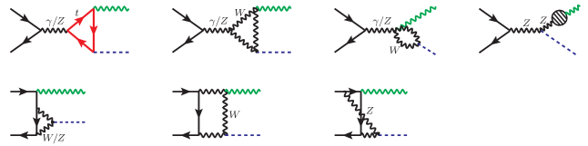
Figure 1: Representative Feynman diagrams for $e^{+}e^{-}\to H\gamma$ at lowest order in SM. The shaded circle in the fourth diagram, which designates one-loop diagrams routed with charge particles, mediates the mixing between $Z^{0}$ and $\gamma$.

This process first occurs at one-loop order in SM, with some typical diagrams shown in Figure 1. The calculation of the LO amplitude has been comprehensively described in Refs. [17, 18, 19].

To assess the impact of the NLO QCD corrections, it is convenient to expand the scalar form factors $C_{1,2}^{\pm}$ in powers of the strong coupling constant:

$${}C_{1,2}^{\pm}=C_{1,2}^{\pm(0)}+\frac{\alpha_{s}}{\pi}C_{1,2}^{\pm(1)}+\cdots,$$ (4)

where $C_{1,2}^{\pm(0)}$ designate the LO contributions, and $C_{1,2}^{\pm(1)}$ encode the relative order-$\alpha_{s}$ corrections.

Substituting (4) back into (3), employing $|C_{1,2}^{\pm}|^{2}\approx|C_{1,2}^{\pm(0)}|^{2}+2{\alpha_{s}\over\pi}\,{\rm Re}\left[C_{1,2}^{\pm(0)}C_{1,2}^{\pm(1)*}\right]$, one then readily identifies the NLO QCD corrections to the differential cross section. The LO expressions for $C_{1,2}^{\pm(0)}$ are well recorded in literatures [17, 18, 19]. The central challenge of this work is then to compute the four form factors $C_{1,2}^{\pm}$ through order $\alpha_{s}$.

In our calculation, we employ the Feynman gauge in both electroweak and QCD sectors. Moreover, we adopt the dimensional regularization to regularize both UV and IR divergences. The LO and NLO Feynman diagrams and corresponding amplitudes are generated by FeynArts [40]. We use the Mathematica packages FeynCalc [41, 42]/FeynCalcFormLink [43] to carry out the trace over Dirac/color matrices, and utilize the packages Apart [44] (and another private code) and the C++ package FIRE [45] to carry out the partial fraction together with the integration-by-parts (IBP) reduction for tensor integrals, finally end up with a number of master integrals (MIs).

Similar to the loop-induced processes $H\to\gamma\gamma,Z\gamma$, the LO amplitude for $e^{+}e^{-}\to H\gamma$ is also UV finite. The corresponding $C_{1,2}^{\pm(0)}$ can then be expressed in terms of the linear combinations of a number of one-loop Passarino-Veltman functions. These form factors have been presented in this format in previous work [19], while retaining a non-vanishing electron mass to regulate the potential collinear divergence (which can arise from the last diagram in Figure 1). Of course, the ultimate amplitude is free from collinear singularity and one is allowed to take the smooth limit $m_{e}\to 0$ in the end. As stated before, we have set $m_{e}=0$ at the outset and used dimensional regularization to regularize both UV and collinear divergences. We feel that our procedure looks simpler both conceptually and technically. For the sake of completeness, and for readers’ convenience, we present our condensed expressions for $C_{1,2}^{\pm(0)}$ in the Appendix. The involved Passarino-Veltman functions can be worked out analytically, or can be accurately evaluated by the packages LoopTools [46] and Collier [47] in a numerical manner.

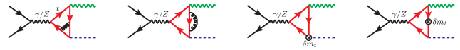
Figure 2: Typical Feynman diagrams for the NLO QCD corrections to $e^{+}e^{-}\to H\gamma$. The cap signifies the insertion of the top quark mass counterterm $\delta m_{t}$, as given in (7).

We wish to describe more details about the calculation of the NLO QCD corrections. At NLO, all the two-loop diagrams have simple $s$-channel topology, some of which are illustrated in Figure 2. They can simply be obtained by dressing the gluon to the top quark loop in all possible ways. For simplicity, we have suppressed the contributions from five lighter quarks, due to their much smaller Yukawa couplings. Thanks to the simple $s$-channel topology, the amplitude assumes a factorized form:

$$\mathcal{M}^{(1)}=e\bar{v}(p_{+})\gamma_{\mu}\bigg{(}g_{e}^{-}P_{-}+g_{e}^{+}P_{+}\bigg{)}u(p_{-}){1\over s-M_{Z}^{2}}\mathcal{T}_{Z\gamma H}^{\mu\nu}\varepsilon_{\gamma,\nu}^{*}+e\bar{v}(p_{+})\gamma_{\mu}u(p_{-}){1\over s}\mathcal{T}_{\gamma\gamma H}^{\mu\nu}\varepsilon_{\gamma,\nu}^{*},$$ (5)

where $P_{\pm}=\frac{1\pm\gamma_{5}}{2}$ are the chirality projection operators. $g_{f}^{-}\equiv I^{3}_{f}/(s_{W}c_{W})-Q_{f}s_{W}/c_{W}$, and $g_{f}^{+}\equiv-Q_{f}s_{W}/c_{W}$, are the $Zf\bar{f}$ couplings for the left-handed and right-handed fermion $f$, respectively, where $Q_{f}$ and $I^{3}_{f}$ designate the corresponding electric charge and the third component of the weak isospin of the fermion $f$. $c_{W}(s_{W})$ stands for the cosine (sine) of the Weinberg angle. The two terms in (5) stem from two distinct channels, $e^{+}e^{-}\to Z^{*}\to H\gamma$ and $e^{+}e^{-}\to\gamma^{*}\to H\gamma$, respectively. $\mathcal{T}_{V\gamma H}^{\mu\nu}$ represent the corresponding tensor form factors related to the $V\gamma H$ ($V=\gamma,Z$) vertex.

As mentioned before, at NLO, we only need consider the contribution to the ${V\gamma H}$ vertex from the top quark loop. Lorentz covariance enables us to parameterize the vertex form factors $\mathcal{T}_{V\gamma H}^{\mu\nu}$ ($V=\gamma,Z$) as

$$\mathcal{T}_{V\gamma H}^{\mu\nu}=T_{V,1}p_{\gamma}^{\mu}p_{\gamma}^{\nu}+T_{V,2}k^{\mu}k^{\nu}+T_{V,3}p_{\gamma}^{\mu}k^{\nu}+T_{V,4}k^{\mu}p_{\gamma}^{\nu}+T_{V,5}p_{\gamma}\cdot kg^{\mu\nu}+T_{V,6}\epsilon^{\mu\nu\alpha\beta}k_{\alpha}p_{\gamma,\beta},$$ (6)

where $k=p_{\gamma}+p_{H}$ is the 4-momentum of the virtual gauge boson $V$, and $T_{V,i}$ ($i=1,\ldots,6$) are various scalar form factors as the functions of $s$ and $m_{H}$. Furry’s theorem, equivalently the charge conjugation symmetry, forbids the axial vector coupling of $Zt\bar{t}$ to yield a nonvanishing contribution (at least at this order), consequently $T_{V,6}=0$. Electromagnetic current conservation implies that $T_{V,2}=0$, and $T_{V,3}=-T_{V,5}$. Furthermore, after substituting (6) into (5), one finds that $T_{V,1}$ and $T_{V,4}$ do not contribute to the amplitude. Consequently, we just need to calculate a single scalar form factor $T_{V,5}$. We emphasize that, the mere QCD renormalization required in this work is to implement the top quark mass renormalization, with the mass counterterm:

$$\delta m_{t}=-\frac{3C_{F}}{4}\frac{\alpha_{s}}{\pi}\bigg{[}\frac{1}{\epsilon}+\frac{4}{3}+\ln\frac{4\pi\mu^{2}}{m_{t}^{2}}-\gamma_{E}\bigg{]}m_{t},$$ (7)

where the spacetime dimensions $d=4-2\epsilon$, and $m_{t}$ signifies the top quark pole mass. The counterterm diagrams are represented by the last two diagrams in Figure 2.

Having eliminated the UV divergences in $T_{V,5}$ ($V=Z,\gamma$) that enter the NLO amplitude in (5), after some straightforward manipulations, one can identify the NLO coefficients $C_{1,2}^{\pm(1)}$ with

$$C_{1}^{\pm(1)}=C_{2}^{\pm(1)}=\frac{e}{2}g_{e}^{\mp}\frac{1}{s-M_{Z}^{2}}T_{Z,5}+\frac{e}{2s}T_{\gamma,5}={e\over 2s}\left(1+g_{e}^{\mp}\kappa{s\over s-M_{Z}^{2}}\right)T_{\gamma,5},$$ (8)

where $\kappa\equiv T_{Z,5}/T_{\gamma,5}=-\tfrac{g_{t}^{+}+g_{t}^{-}}{2Q_{t}}$. It is easy to understand why $T_{Z,5}$ and $T_{\gamma,5}$ are proportional to each other, since only the vector part of the $Zt\bar{t}$ coupling survives in the amplitude. Plugging (8) into (4) and (3), we then deduce the desired NLO QCD corrections to the differential cross section.

We pause here to briefly describe our numerical strategy of computing the NLO corrections. After IBP reduction, we end up with about 34 two-loop MIs for $T_{\gamma,5}$. For each MI, we combine FIESTA [48]/CubPack [49] to perform the sector decomposition and the subsequent numerical integrations with quadruple precision. We also utilize the Fortran package Cuba [50] to crosscheck the numerical integrations for most MIs.

It is worth mentioning that our two-loop calculation is quite similar to the corresponding calculation for the rare decay process $H\to Z\gamma$. The NLO QCD corrections to that process were recently accomplished by two groups in an analytic fashion [38, 39]. As a crosscheck, we have also revisited that process and found good agreement with the numerical results tabulated in [38]. Having passed such a nontrivial test, we feel confident about the correctness of our NLO QCD calculation for $e^{+}e^{-}\to H\gamma$.

In principle, our $T_{Z,5}$ can be obtained from its counterpart in $H\to Z\gamma$ by performing some sort of analytic continuation. Unfortunately, the analytic expressions recorded in Refs. [38, 39] involve rather lengthy and complicated special functions, rendering analytic continuation a rather nontrivial task. Therefore, we are contented with only presenting the highly accurate numerical predictions in this Letter.

3 Numerical results

In order to make concrete predictions, we specify the following input parameters, in accordance with the latest compilation of the Particle Data Group [51]:

$$M_{W}=80.385\,{\rm GeV},\,\,M_{Z}=91.1876\,{\rm GeV},\,\,m_{t}=174.2\,{\rm GeV},\,\,$$

$$m_{H}=125.09\,{\rm GeV},\,\,\alpha=1/{137.035999}.$$ (9)

In addition, the default renormalization scale $\mu=\sqrt{s}$ is assumed for the QCD running coupling constant $\alpha_{s}(\mu)$. We take the initial value $\alpha_{s}^{(5)}(M_{Z})=0.118$, and use the two-loop running formula to evolve to another different energy scale. Practically, it is very convenient to utilize the package RunDec [52], which has automated the evolution of the QCD running coupling and taken care of the top quark threshold effect.

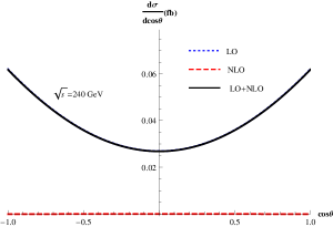
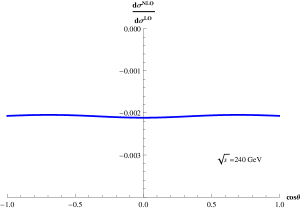
Figure 3: Angular distributions of the Higgs boson in the $e^{+}e^{-}\to H\gamma$ process at $\sqrt{s}=240$ GeV. The right panel embodies the relative magnitude of the NLO QCD corrections.

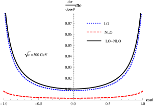
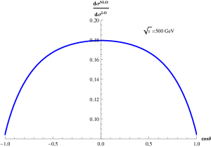
Figure 4: Angular distributions of the Higgs boson in the $e^{+}e^{-}\to H\gamma$ process at $\sqrt{s}=500$ GeV. The right panel signifies the relative magnitude of the NLO QCD corrections.

Before proceeding into phenomenological discussions, we should remind the readers that our LO predictions are subject to an intrinsic ambiguity due to the choice of the electroweak coupling constants. In this work, we have chosen to use the Thomson-limit value of QED coupling $\alpha(0)$. Certainly, it is equally legitimate to adopt different values for $\alpha$, such as the widely-used $\alpha_{G_{\mu}}$ and $\alpha(M_{Z})$ [53]. This uncertainty might be even more pronounced than the size of the NLO QCD corrections. This ambiguity can only be lessened once one incorporates the full NLO weak corrections, unfortunately which is currently unavailable.

In Figure 3 and 4, we plot the angular distributions of the Higgs boson at two benchmark CM energy points, $\sqrt{s}=240$ GeV at CEPC, and 500 GeV at ILC. As the CM energy increases, the angular distributions turn to be more and more concentrated in the forward/backward directions. As one can readily tell, the effect of NLO QCD corrections at CEPC energy, which only constitutes $\sim 0.2\%$ of the LO contribution, is hardly discernible. In the meanwhile, the impact of the NLO QCD corrections becomes clearly visible at ILC energy range.

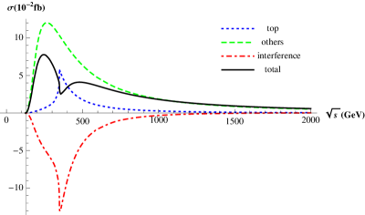
Figure 5: The LO cross section as a function of $\sqrt{s}$ (the solid line). To trace the origin of the nontrivial line shape, we deliberately isolate the contributions from two classes of diagrams. The dotted, dashed and dot-dashed lines represent the contribution from diagrams involving the top quark loop, that from all other diagrams involving weak gauge bosons in the loop, and their interference, respectively.

To ascertain the integrated cross section at each CM energy point, we utilize Cuba [50] to carry out the angular integration numerically. In Figure 5, the variation of the LO cross section with the CM energy is depicted over a wide range. There the line shape exhibits some interesting features. Starting from the threshold $\sqrt{s}=m_{H}$, the cross section rises from zero due to the increment of the phase space. The cross section reaches its first peak around $\sqrt{s}=245$ GeV, followed by a dip around $\sqrt{s}=359$ GeV, then slowly bounces up and reaches the second lower peak centered at $\sqrt{s}=480$ GeV. The cross section then decreases monotonically with increasing $\sqrt{s}$.

To understand the origin of the peak-dip-peak structure, we separate the contributions into two categories, those from the diagrams involving the top quark loop and from the diagrams involving electroweak gauge bosons. There arises a cusp from the former channel, exactly located at the $t\bar{t}$ threshold $\sqrt{s}=2m_{t}=348.4$ GeV. From Figure 5, one observes that there arises a substantial destructive interference between these two channels, whose effects reach the maximum at $\sqrt{s}\approx 352$ GeV. This destructive interference seems to be largely responsible for the global minimum of the net LO line shape. It is interesting to note that the location of this dip deviates from the $t\bar{t}$ threshold by 10 GeV.

We wish to understand the asymptotic behavior of $\sigma(H\gamma)$ in the high energy limit. For this purpose, it is instructive to temporarily digress into the asymptotic scaling of the total cross section of a similar Higgs production channel, the Higgsstrahlung process. It is well-known that $\sigma(HZ)$ scales as $1/s$ in the high energy limit [12, 13, 14]. This scaling is saturated by the channel with a longitudinally-polarized $Z$, while the polarized cross section for a transversely-polarized $Z$ declines at a much steeper rate, $\propto 1/s^{2}$ [14, 15].

Since the photon must be transversely polarized, one might naively anticipate that $\sigma(H\gamma)$ should decrease as $1/s^{2}$ asymptotically. However, a careful numerical investigation reveals that this expectation is not true! At sufficiently high energy, the cross section turns out to decline with a much slower pace, $\propto 1/s$. In addition to this power-law scaling, we have not observed any hint of logarithmic enhancement, to a decent numerical accuracy. Therefore, the $\ln^{n}s$ ($n=1,2$) terms, if exist, must be accompanied with the power-suppressed terms ($\propto 1/s^{2}$).

It is interesting to trace the origin for the $1/s$ scaling of $\sigma(H\gamma)$ at high energy. Note there is one important difference between Higgsstrahlung and the process considered in this Letter, e.g., the former starts at tree level, but the latter starts at one loop order. The $s$-channel diagrams in Figure 1 indeed only yield a suppressed contribution $\propto 1/s^{2}$, modulo possible logarithms of $s$. Nevertheless, the box diagrams in Figure 1, which are responsible for the sharp concentration of the differential cross sections in the forward/backward zones, will bring forth an enhancement factor $\propto{s\over M^{2}}$ (here $M$ refers to a generic mass scale of order $M_{Z,W}$ or $M_{H}$) upon angular integration. A closer analytic examination also supports the absence of logarithms of $s$ accompanying this leading-power scaling.

$\sqrt{s}({\rm GeV})$	150	200	220	240	250	270	290	310	330	340
$\sigma^{{\rm LO}}$ ($10^{-2}$ fb)	1.054	6.214	7.339	7.758	$7.764$	$7.479$	$6.909$	$6.134$	$5.151$	4.522
$\widetilde{T}_{\gamma,5}$($10^{-2}$GeV-1)	-0.793	-0.378	-0.112	0.251	0.485	1.12	2.11	3.90	8.16	14.26
$\sigma^{{\rm NLO}}/\sigma^{{\rm LO}}$	0.56%	0.30%	0.09%	-0.21%	-0.41%	-0.96%	-1.86%	-3.45%	-6.85%	-10.59%
$\sqrt{s}({\rm GeV})$	360	380	400	420	500	600	700	800	900	1000
$\sigma^{{\rm LO}}$ ($10^{-2}$ fb)	2.570	2.977	3.433	3.763	4.079	3.604	3.018	2.518	2.118	1.801
$\widetilde{T}_{\gamma,5}$ ($10^{-2}$GeV-1)	$-2.26$	$-11.6$	$-13.4$	$-13.24$	$-9.65$	$-6.31$	$-4.45$	$-3.35$	$-2.63$	$-2.13$
	$+28.2\,i$	$+16.6\,i$	$+9.81\,i$	$+5.76\,i$	$-1.29\,i$	$-3.21\,i$	$-3.48\,i$	$-3.38\,i$	$-3.19$ i	$-3.00\,i$
$\sigma^{{\rm NLO}}/\sigma^{{\rm LO}}$	-4.99%	16.81%	19.87%	19.24%	13.67%	9.60%	7.37%	5.98%	5.02%	4.31%

Table 1: The integrated cross sections of $e^{+}e^{-}\to H\gamma$ in a variety range of CM energy, at both LO and NLO accuracy. We also enumerate the corresponding values of the scalar form factors $T_{\gamma,5}$ in (8). For simplicity, we have eliminated the $\alpha$-dependence by redefining $\widetilde{T}_{\gamma,5}\equiv\alpha^{-3/2}\,T_{\gamma,5}$.

In Table 1 we enumerate the predicted cross sections over a wide range of CM energy, at both LO and NLO accuracy. In addition, we also tabulate the values of the scalar form factors $T_{\gamma,5}$ at various CM energies. At CEPC energy range, $\sqrt{s}\approx 250$ GeV, the NLO QCD corrections have a negligible effect. In contrast, if the ILC and FCC-ee operate at $\sqrt{s}\approx 400$ GeV, the magnitude of the NLO QCD corrections could reach roughly $20\%$ of the LO cross section.

As can be noticed in Table 1, as $\sqrt{s}>2m_{t}$, the two-loop form factor $T_{\gamma,5}$ develops an imaginary part due to the opening of the $t\bar{t}$ threshold. Through an exhaustive threshold scan, we observe that the real part of $T_{\gamma,5}$ develops a logarithmic singularity $\propto\ln|\beta|$ ($\beta\equiv\sqrt{1-{4m_{t}^{2}\over s}}$) in the vicinity of the threshold, while the imaginary part approaches a constant above from the $t\bar{t}$ threshold. This is a clear sign that the nearly-on-shell $t\bar{t}$ pair in the loop carries the dominant quantum number of ${}^{3}S_{1}$. It is well-known in such a case, the Coulomb singularity $\propto{1\over\beta}$ will arise for even higher-order diagrams containing more Coulomb gluon exchange, so that fixed-order QCD perturbative expansion inevitably breaks down near the threshold. For inclusive $t\bar{t}$ production near the threshold, a vast amount of literatures have been devoted to providing a systematic description in the threshold region, by resumming Coulomb singularities to all orders and incorporating the finite $t$ width effect, in the context of non-relativistic effective field theory NRQCD [54, 55, 56, 57, 58]. For our exclusive $H+\gamma$ process, one may closely follow the ansatz adopted for the pseudosalar Higgs decay into two photons when the pseudoscalar Higgs mass is about twice the top quark mass, where a $t\bar{t}$ pair is in the ${}^{1}S_{0}$ state in the loop [59, 60]. The resummation of the Coulomb gluon ladder diagrams, as well as including top quark width, could also be readily fulfilled, so that one can obtain reliable predictions for $\sigma(H\gamma)$ in the vicinity of $\sqrt{s}=2m_{t}$. Such a “nonperturbative” treatment is beyond the scope of this Letter, and we plan to present a comprehensive threshold analysis for this process in the near future. In any rate, our fixed-order predictions recorded in Table 1, should still be viewed as trustworthy, as long as $\sqrt{s}$ does not lie in proximity to the $t\bar{t}$ threshold.

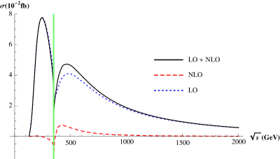
Figure 6: The total cross section as a function of $\sqrt{s}$, both at LO and NLO in $\alpha_{s}$. The vertical band with $\sqrt{s}=2m_{t}\pm 5$ GeV signifies the threshold region, inside which the perturbative expansion is expected to break down and our fixed-order predictions become invalid.

For the sake of clarity, in Figure 6 we also plot the integrated cross section as a function of the CM energy, explicitly including the NLO QCD corrections. In most energy ranges, the impact of the NLO QCD corrections seems rather modest, especially when $\sqrt{s}<290$ GeV, with a relative effect typically less than $1\%$. Nevertheless, with the increasing CM energy, the QCD corrections appear to become more pronounced, and reach the maximum about 20% at $\sqrt{s}\approx 400$ GeV. The effect of NLO corrections diminishes again as the CM energy further increases, completely negligible after $\sqrt{s}>1$ TeV. This can be readily understood in light of the preceding discussions: due to the dominance of the electroweak box diagrams, the LO cross section exhibits a mild $1/s$ asymptotic scaling, while the NLO QCD corrections fall with a much faster pace $\propto 1/s^{2}$, since the corresponding diagrams possess only $s$-channel topology.

$m_{H}({\rm GeV})$	40	60	80	100	120	140	160	180	200	220
$\sigma^{{\rm LO}}$ ($10^{-2}$ fb)	$15.46$	$14.15$	$12.43$	$10.42$	$8.293$	$6.288$	$5.454$	$3.212$	$1.170$	$0.1659$
$\tilde{T}_{\gamma,5}$($10^{-4}$GeV-1)	-3.70	0.101	5.59	12.9	22.3	34.2	48.9	67.1	89.7	118
$\sigma^{{\rm NLO}}/\sigma^{{\rm LO}}$	0.03%	-0.001%	-0.05%	-0.11%	-0.19%	-0.27%	-0.33%	-0.40%	-0.48%	-0.58%

Table 2: Cross sections of $e^{+}e^{-}\to H\gamma$ as a function of Higgs boson mass, with $\sqrt{s}$ fixed at 240 GeV.

Finally in Table 2, we further study the dependence of the NLO QCD corrections on the Higgs boson mass, with $\sqrt{s}$ held at 240 GeV. The LO cross section decreases monotonously with the rising $m_{H}$, partly due to the shrinking phase space. The magnitude of the NLO QCD corrections varies with $m_{H}$ with a modest pace, nevertheless always less significant than $1\%$.

4 Summary and Outlook

The LO predictions for the production rate of $e^{+}e^{-}\to H\gamma$ in SM are rather small at the next-generation $e^{+}e^{-}$ colliders, which may render it a sensitive probe for the elusive beyond-SM signals. An accurate account of this process within SM appears mandatory, if one wishes to confidently confront the potential new physics signals in the future. In this Letter, we have, for the first time, calculated the NLO QCD corrections to this associated $H+\gamma$ production process, and conducted a comprehensive numerical study covering a wide range of CM energy. The key finding is that, the NLO QCD corrections to this process at CEPC can be safely neglected, but may have sizable impact at ILC energy range. Nevertheless, the $e^{+}e^{-}\to H\gamma$ process appears to possess the maximal production rate, $\sigma_{\rm max}\approx 0.08$ fb, around $\sqrt{s}=250$ GeV, therefore CEPC appears to be the ideal place to look for this rare Higgs production process.

It may also be valuable to reanalyze this process for polarized electron beam, as is useful for the ILC experiment.

As was mentioned before, in order to obtain a precise prediction for the $e^{+}e^{-}\to H\gamma$ process, it seems mandatory to lessen the large ambiguity inherent in the choice of the electroweak coupling constants. This symptom can only be relieved by further including the NLO weak corrections. As was witnessed in the Higgsstrahlung process, incorporating the NLO weak corrections does significantly stabilize the predicted production rate for $HZ$ [14, 15]. This is particularly important for our process, since the ambiguity due to the choice of $\alpha$ might even bring forth greater uncertainty than the magnitude of NLO QCD corrections per se. Despite its daunting difficulty, we hope that future fulfillment of the NLO weak corrections to this process will significantly reduce the $\alpha$-scheme dependence. Combined with the NLO QCD corrections calculated in this Letter, we will then be able to provide a fairly reliable guidance for the future experimental search of this rare Higgs production channel.

Finally, we think it is also of some interest to conduct a full-fledged study for $\sigma(H\gamma)$ in the vicinity of the $t\bar{t}$ threshold, which necessitates to include resummation of the Coulomb gluon ladder diagrams and top quark width effect.

Appendix: The compact expressions for $C^{\pm(0)}_{1,2}$

For reader’s convenience, here we list the compact expressions for the LO coefficients functions $C^{\pm(0)}_{1,2}$ appearing in (3), with $m_{e}$ set to zero at the outset. They can be split into three parts:

$$C^{\pm(0)}_{i}=\alpha^{2}\bigg{[}\sum_{V=Z,\gamma}\frac{g^{\mp}_{Ve}M_{W}}{2s_{W}(s-M_{V}^{2})}C^{\pm(0,{\rm vert})}_{Vi}-\frac{M_{W}}{s_{W}^{3}}C^{\pm(0,{\rm Wbox})}_{i}+\frac{2M_{W}}{s_{W}c_{W}^{2}}C^{\pm(0,{\rm Zbox})}_{i}\bigg{]},$$ (10)

where $i=1,2$, and

$$C^{\pm(0,\text{vert})}_{Vi} =\frac{4}{3}\frac{m_{t}^{2}}{M_{W}^{2}}N_{c}\left(g_{Vt}^{-}+g_{Vt}^{+}\right)\left(C_{0}^{a}+4C_{2}^{a}+4C_{12}^{a}+4C_{22}^{a}\right)$$ (11f)

$$+4\frac{m_{H}^{2}}{M_{W}^{2}}c_{V2}\left(C_{2}^{b}+C_{12}^{b}+C_{22}^{b}\right)+c_{V1}\left(10C_{0}^{b}-2C_{1}^{b}+17C_{2}^{b}+19C_{12}^{b}+19C_{22}^{b}\right)$$

$$+2c_{V2}\left(2C_{0}^{b}+2C_{1}^{b}+3C_{2}^{b}+C_{12}^{b}+C_{22}^{b}\right)+c_{V3}\left(2C_{0}^{b}-2C_{1}^{b}+C_{2}^{b}+3C_{12}^{b}+3C_{22}^{b}\right),\phantom{xxxx}$$

$$C^{+(0,{\rm Wbox})}_{1}=D_{2}^{a}+D_{23}^{a}+D_{2}^{b}-D_{23}^{b}-D_{33}^{b},$$

$$C^{+(0,{\rm Wbox})}_{2}=D_{1}^{a}+D_{1}^{b}+D_{13}^{b}-D_{13}^{a}-D_{33}^{a},$$

$$C^{-(0,{\rm Wbox})}_{1,2}=0,$$

$$C^{\pm(0,{\rm Zbox})}_{1}=-g_{e}^{\mp 2}\left(D_{13}^{c}+D_{33}^{c}\right),$$

$$C^{\pm(0,{\rm Zbox})}_{2}=g_{e}^{\mp 2}\left(D_{2}^{c}+D_{12}^{c}+D_{23}^{c}\right),$$

where $g^{\pm}_{Zf}=g^{\pm}_{f},g^{\pm}_{\gamma f}=-Q_{f}$, and we define $c_{Z1}\equiv-c_{W}/s_{W}$, $c_{Z2}\equiv(s_{W}^{2}-c_{W}^{2})/(2s_{W}c_{W})$, $c_{Z3}\equiv s_{W}/c_{W}$, $c_{\gamma 1}=c_{\gamma 2}=c_{\gamma 3}\equiv 1$, and

$$C^{a}_{ij\ldots} \equiv C_{ij\ldots}(0,s,m_{H}^{2},m_{t}^{2},m_{t}^{2},m_{t}^{2}),$$ (12a)

$$C_{ij\ldots}^{b} \equiv C_{ij\ldots}(0,s,m_{H}^{2},M_{W}^{2},M_{W}^{2},M_{W}^{2}),$$ (12b)

$$D_{ij\ldots}^{a} \equiv D_{ij\ldots}(0,s,m_{H}^{2},u,0,0,0,M_{W}^{2},M_{W}^{2},M_{W}^{2}),$$ (12c)

$$D_{ij\ldots}^{b} \equiv D_{ij\ldots}(0,s,0,t,0,m_{H}^{2},0,M_{W}^{2},M_{W}^{2},M_{W}^{2}),$$ (12d)

$$D_{ij\ldots}^{c} \equiv D_{ij\ldots}(0,u,m_{H}^{2},t,0,0,0,0,M_{Z}^{2},M_{Z}^{2}).$$ (12e)

We use the same conventions for the Passarino-Veltman scalar functions as in most modern literatures (see, for instance, Ref. [47]). Note that the functions (12e), which originate from the last diagram in Figure 1, are by themselves free from any collinear singularity. However, if the IBP reduction is further implemented to (12e), one will end up with a linear combination of a number of one-loop scalar MIs, some of which are IR divergent. Fortunately, one can use LoopTools [46] and Collier [47] to directly calculate these Passarino-Veltman functions in (12).

References

- [1] G. Aad et al. [ATLAS Collaboration], Phys. Lett. B 716 (2012) 1 [arXiv:1207.7214 [hep-ex]].
- [2] S. Chatrchyan et al. [CMS Collaboration], Phys. Lett. B 716 (2012) 30 [arXiv:1207.7235 [hep-ex]].
- [3] G. Aad et al. [ATLAS and CMS Collaborations], JHEP 1608 (2016) 045 [arXiv:1606.02266 [hep-ex]].
- [4] H. Baer et al., arXiv:1306.6352 [hep-ph].
- [5] D. M. Asner et al., arXiv:1310.0763 [hep-ph].
- [6] M. Bicer et al. [TLEP Design Study Working Group Collaboration], JHEP 1401, 164 (2014) [arXiv:1308.6176 [hep-ex]], http://tlep.web.cern.ch/
- [7] CEPC-SPPC Study Group, IHEP-CEPC-DR-2015-01, IHEP-TH-2015-01, HEP-EP-2015-01.
- [8] CEPC-SPPC Study Group, IHEP-CEPC-DR-2015-01, IHEP-AC-2015-01.
- [9] J. R. Ellis, M. K. Gaillard and D. V. Nanopoulos, Nucl. Phys. B 106, 292 (1976).
- [10] B. L. Ioffe and V. A. Khoze, Sov. J. Part. Nucl. 9, 50 (1978) [Fiz. Elem. Chast. Atom. Yadra 9, 118 (1978)].
- [11] J. D. Bjorken, Conf. Proc. C 7608021, 1 (1976).
- [12] J. Fleischer and F. Jegerlehner, Nucl. Phys. B 216 (1983) 469.
- [13] B. A. Kniehl, Z. Phys. C 55 (1992) 605.
- [14] A. Denner, J. Kublbeck, R. Mertig and M. Bohm, Z. Phys. C 56 (1992) 261.
- [15] Q. F. Sun, F. Feng, Y. Jia and W. L. Sang, Phys. Rev. D 96, 051301(R) (2017) [arXiv:1609.03995 [hep-ph]].
- [16] Y. Gong, Z. Li, X. Xu, L. L. Yang and X. Zhao, Phys. Rev. D 95, 093003 (2017) [arXiv:1609.03955 [hep-ph]].
- [17] A. Barroso, J. Pulido and J. C. Romao, Nucl. Phys. B 267 (1986) 509.
- [18] A. Abbasabadi, D. Bowser-Chao, D. A. Dicus and W. W. Repko, Phys. Rev. D 52 (1995) 3919 [hep-ph/9507463].
- [19] A. Djouadi, V. Driesen, W. Hollik and J. Rosiek, Nucl. Phys. B 491 (1997) 68 [hep-ph/9609420].
- [20] G. J. Gounaris, F. M. Renard and N. D. Vlachos, Nucl. Phys. B 459 (1996) 51 [hep-ph/9509316].
- [21] U. Mahanta, Phys. Lett. B 423 (1998) 126.
- [22] A. Arhrib, R. Benbrik and T. C. Yuan, Eur. Phys. J. C 74 (2014) 2892 [arXiv:1401.6698 [hep-ph]].
- [23] S. L. Hu, N. Liu, J. Ren and L. Wu, J. Phys. G 41 (2014) no.12, 125004 [arXiv:1402.3050 [hep-ph]].
- [24] H. Y. Ren, Chin. Phys. C 39 (2015) no.11, 113101 [arXiv:1503.08307 [hep-ph]].
- [25] Q. H. Cao, H. R. Wang and Y. Zhang, Chin. Phys. C 39 (2015) no.11, 113102 [arXiv:1505.00654 [hep-ph]].
- [26] G. Li, H. R. Wang and S. h. Zhu, Phys. Rev. D 93 (2016) no.5, 055038 [arXiv:1506.06453 [hep-ph]].
- [27] H. Q. Zheng and D. D. Wu, Phys. Rev. D 42 (1990) 3760.
- [28] A. Djouadi, M. Spira, J. J. van der Bij and P. M. Zerwas, Phys. Lett. B 257 (1991) 187.
- [29] S. Dawson and R. P. Kauffman, Phys. Rev. D 47 (1993) 1264.
- [30] A. Djouadi, M. Spira and P. M. Zerwas, Phys. Lett. B 311 (1993) 255 [hep-ph/9305335].
- [31] K. Melnikov and O. I. Yakovlev, Phys. Lett. B 312 (1993) 179 [hep-ph/9302281].
- [32] M. Inoue, R. Najima, T. Oka and J. Saito, Mod. Phys. Lett. A 9 (1994) 1189.
- [33] M. Spira, A. Djouadi, D. Graudenz and P. M. Zerwas, Nucl. Phys. B 453 (1995) 17 [hep-ph/9504378].
- [34] J. Fleischer, O. V. Tarasov and V. O. Tarasov, Phys. Lett. B 584 (2004) 294 [hep-ph/0401090].
- [35] R. Harlander and P. Kant, JHEP 0512 (2005) 015 [hep-ph/0509189].
- [36] U. Aglietti, R. Bonciani, G. Degrassi and A. Vicini, JHEP 0701 (2007) 021 [hep-ph/0611266].
- [37] M. Spira, A. Djouadi and P. M. Zerwas, Phys. Lett. B 276 (1992) 350.
- [38] R. Bonciani, V. Del Duca, H. Frellesvig, J. M. Henn, F. Moriello and V. A. Smirnov, JHEP 1508 (2015) 108 [arXiv:1505.00567 [hep-ph]].
- [39] T. Gehrmann, S. Guns and D. Kara, JHEP 1509, 038 (2015) [arXiv:1505.00561 [hep-ph]].
- [40] T. Hahn, Comput. Phys. Commun. 140, 418 (2001) [hep-ph/0012260].
- [41] R. Mertig, M. Bohm and A. Denner, Comput. Phys. Commun. 64, 345 (1991).
- [42] V. Shtabovenko, R. Mertig and F. Orellana, Comput. Phys. Commun. 207 (2016) 432 [arXiv:1601.01167 [hep-ph]].
- [43] F. Feng and R. Mertig, arXiv:1212.3522.
- [44] F. Feng, Comput. Phys. Commun. 183, 2158 (2012) [arXiv:1204.2314 [hep-ph]].
- [45] A. V. Smirnov, Comput. Phys. Commun. 189, 182 (2014) [arXiv:1408.2372 [hep-ph]].
- [46] T. Hahn and M. Perez-Victoria, Comput. Phys. Commun. 118, 153 (1999) [hep-ph/9807565].
- [47] A. Denner, S. Dittmaier and L. Hofer, Comput. Phys. Commun. 212 (2017) 220 [arXiv:1604.06792 [hep-ph]].
- [48] A. V. Smirnov, Comput. Phys. Commun. 204 (2016) 189 [arXiv:1511.03614 [hep-ph]].
- [49] R. Cools and A. Haegemans, ACM Trans. Math. Softw. 29 (2003), no. 3 287 C296.
- [50] T. Hahn, Comput. Phys. Commun. 168 (2005) 78 [hep-ph/0404043].
- [51] C. Patrignani et al. [Particle Data Group], Chin. Phys. C 40 (2016) no.10, 100001.
- [52] K. G. Chetyrkin, J. H. Kuhn and M. Steinhauser, Comput. Phys. Commun. 133, 43 (2000) [hep-ph/0004189].
- [53] A. Denner, Fortsch. Phys. 41, 307 (1993) [arXiv:0709.1075 [hep-ph]].
- [54] V. S. Fadin and V. A. Khoze, JETP Lett. 46 (1987) 525 [Pisma Zh. Eksp. Teor. Fiz. 46 (1987) 417].
- [55] V. S. Fadin and V. A. Khoze, Sov. J. Nucl. Phys. 48 (1988) 309 [Yad. Fiz. 48 (1988) 487].
- [56] M. J. Strassler and M. E. Peskin, Phys. Rev. D 43 (1991) 1500.
- [57] A. H. Hoang et al., Eur. Phys. J. direct 2, no. 1, 3 (2000) [hep-ph/0001286].
- [58] M. Beneke, Y. Kiyo, P. Marquard, A. Penin, J. Piclum and M. Steinhauser, Phys. Rev. Lett. 115, no. 19, 192001 (2015) [arXiv:1506.06864 [hep-ph]].
- [59] M. Drees and K. i. Hikasa, Phys. Rev. D 41, 1547 (1990).
- [60] K. Melnikov, M. Spira and O. I. Yakovlev, Z. Phys. C 64, 401 (1994) [hep-ph/9405301].
- [61] D. Binosi and L. Theussl, Comput. Phys. Commun. 161, 76 (2004) [hep-ph/0309015].
- [62] D. Binosi, J. Collins, C. Kaufhold and L. Theussl, Comput. Phys. Commun. 180 (2009) 1709 [arXiv:0811.4113 [hep-ph]].