Kernel partial least squares for stationary data

Abstract

We consider the kernel partial least squares algorithm for non-parametric regression with stationary dependent data. Probabilistic convergence rates of the kernel partial least squares estimator to the true regression function are established under a source and an effective dimensionality conditions. It is shown both theoretically and in simulations that long range dependence results in slower convergence rates. A protein dynamics example shows high predictive power of kernel partial least squares.

Key words and phrases. Effective dimensionality, Long range dependence, Nonparametric regression, Source condition, Protein dynamics.

1 Introduction

Partial least squares (PLS) is a regularized regression technique developed by Wold et al., (1984) to deal with collinearities in the regressor matrix. It is an iterative algorithm where the covariance between response and regressor is maximized at each step, see Helland, (1988) for a detailed description. Regularization in the PLS algorithm is obtained by stopping the iteration process early.

Several studies showed that partial least squares algorithm is competitive with other regression methods such as ridge regression and principal component regression and it needs generally fewer iterations than the latter to achieve comparable estimation and prediction, see, e.g., Frank and Friedman, (1993) and Krämer and Braun, (2007). For an overview of further properties of PLS we refer to Rosipall and Krämer, (2006).

Reproducing kernel Hilbert spaces (RKHS) have a long history in probability and statistics (see e.g. Berlinet and Thomas-Agnan,, 2004). Here we focus on the supervised kernel based learning approach for the solution of non-parametric regression problems. RKHS methods are both computationally and theoretically attractive, due to the kernel trick (Schölkopf et al.,, 1998) and the representer theorem (Wahba,, 1999) as well as its generalization (Schölkopf et al.,, 2001). Within the reproducing kernel Hilbert space framework one can adapt linear regularized regression techniques like ridge regression and principal component regression to a non-parametric setting, see Saunders et al., (1998) and Rosipal et al., (2000), respectively. We refer to Schölkopf and Smola, (2001) for more details on the kernel based learning approach.

Kernel PLS was introduced in Rosipal and Trejo, (2001) who reformulated the algorithm presented in Lindgren et al., (1993). The relationship to kernel conjugate gradient (KCG) methods was highlighted in Blanchard and Krämer, 2010a . It can be seen in Hanke, (1995) that conjugate gradient methods are well suited for handling ill-posed problems, as they arise in kernel learning, see, e.g., De Vito et al., (2006).

Rosipal, (2003) investigated the performance of kernel partial least squares (KPLS) for non-linear discriminant analysis. Blanchard and Krämer, 2010a proved the consistency of KPLS when the algorithm is stopped early without giving convergence rates.

Caponnetto and de Vito, (2007) showed that kernel ridge regression (KRR) attains optimal probabilistic rates of convergence for independent and identically distributed data, using a source and a polynomial effective dimensionality condition. A generalization of these results to a wider class of effective dimensionality conditions and extension to kernel principal component regression can be found in Dicker et al., (2017).

For a variant of KCG Blanchard and Krämer, 2010b obtained probabilistic convergence rates for independent identically distributed data. The pointed explicitly out that their approach and results are not directly applicable to KPLS.

We study of the convergence of the kernel partial least squares estimator to the true regression function when the algorithm is stopped early. Similar to Blanchard and Krämer, 2010b we derive explicit probabilistic convergence rates. In contrast to previously cited works on kernel regression our input data are not independent and identically distributed but rather stationary time series. We derive probabilistic convergence results that can be applied for arbitrary temporal dependence structures, given that certain concentration inequalities for these data hold. The derived convergence rates depend not only on the complexity of the target function and of the data mapped into the kernel space, but also on the persistence of the dependence in the data. In the stationary setting we prove that the short range dependence still leads to optimal rates, but if the dependence is more persistent, the rates become slower.

2 Kernel Partial Least Squares

Consider the non-parametric regression problem

$$y_{t}=f^{\ast}(X_{t})+\varepsilon_{t},\leavevmode\nobreak\ \leavevmode\nobreak\ t\in{\mathbb{Z}}.$$ (1)

Here $\{X_{t}\}_{t\in{\mathbb{Z}}}$ is a $d$-dimensional, $d\in{\mathbb{N}}$, stationary time series on a probability space $(\Omega,\mathcal{A},\mathrm{P})$ and $\{\varepsilon_{t}\}_{t\in{\mathbb{Z}}}$ is an independent and identically distributed sequence of real valued random variables with expectation zero and variance $\sigma^{2}>0$ that is independent of $\{X_{t}\}_{t\in{\mathbb{Z}}}$. Let $X$ be a random vector that is independent of $\{X_{t}\}_{t\in{\mathbb{Z}}}$ and $\{\varepsilon_{t}\}_{t\in{\mathbb{Z}}}$ with the same distribution as $X_{0}$. The target function we seek to estimate is $f^{\ast}\in\mathcal{L}^{2}\left(\mathrm{P}^{X}\right)$.

For the purpose of supervised learning assume that we have a training sample $\{(X_{t},y_{t})\}_{t=1}^{n}$ for some $n\in{\mathbb{N}}$. In the following we introduce some basic notation for the kernel based learning approach.

Define with $(\mathcal{H},\langle\cdot,\cdot\rangle_{\mathcal{H}})$ the RKHS of functions on ${\mathbb{R}}^{d}$ with reproducing kernel $k:{\mathbb{R}}^{d}\times{\mathbb{R}}^{d}\rightarrow{\mathbb{R}}$, i.e., it holds

$$g(x)=\langle g,k(\cdot,x)\rangle_{\mathcal{H}},\leavevmode\nobreak\ \leavevmode\nobreak\ x\in{\mathbb{R}}^{d},g\in\mathcal{H}.$$ (2)

The corresponding inner product and norm in $\mathcal{H}$ is denoted by $\langle\cdot,\cdot\rangle_{\mathcal{H}}$ and $\|\cdot\|_{\mathcal{H}}$, respectively. We refer to Berlinet and Thomas-Agnan, (2004) for examples of Hilbert spaces and their reproducing kernels. In the following we deal with reproducing kernel Hilbert spaces which fulfill the following, rather standard, conditions:

1. $\mathcal{H}$ is separable,

2. There exists a $\kappa>0$ such that $|k(x,y)|\leq\kappa$ for all $x,y\in{\mathbb{R}}^{d}$ and $k$ is measurable.

Under (K1) the Hilbert-Schmidt norm $\|\cdot\|_{\mathrm{HS}}$ for operators mapping from $\mathcal{H}$ to $\mathcal{H}$ is well defined. If condition (K2) holds, all functions in $\mathcal{H}$ are bounded, see Berlinet and Thomas-Agnan, (2004), chapter 2. The conditions are satisfied for a variety of popular kernels, e.g., Gaussian or triangular.

The main principle of RKHS methods is the mapping of the data $X_{t}$ into $\mathcal{H}$ via the feature maps $\phi_{t}=k(\cdot,X_{t})$, $t=1,\dots,n$. This mapping can be done implicitly by using the kernel trick $\langle\phi_{t},\phi_{s}\rangle_{\mathcal{H}}=k(X_{t},X_{s})$ and thus only the $n\times n$ dimensional kernel matrix $K_{n}=n^{-1}[k(X_{t},X_{s})]_{t,s=1}^{n}$ is needed in the computations. Then the task for RKHS methods is to find coefficients $\alpha_{1},\dots,\alpha_{n}$ such that $f_{\alpha}=\sum_{t=1}^{n}\alpha_{t}\phi_{t}$ is an adequate approximation of $f^{\ast}$ in $\mathcal{H}$, measured in the $\mathcal{L}^{2}\left(\mathrm{P}^{X}\right)$ norm $\|\cdot\|_{2}$.

There are a variety of different approaches to estimate the coefficients $\alpha_{1},\dots,\alpha_{n}$, including kernel ridge regression, kernel principal component regression and, of course, kernel partial least squares. The latter method was introduced by Rosipal and Trejo, (2001) and is the focus of the current work.

It was shown by Krämer and Braun, (2007) that the KPLS algorithm solves

$$\widehat{\alpha}_{i}=\arg\min\limits_{v\in\mathcal{K}_{i}(K_{n},y)}\|y-K_{n}v\|^{2},\leavevmode\nobreak\ \leavevmode\nobreak\ i=1,\dots,n,$$ (3)

with $y=(y_{1},\dots,y_{n})^{\mathrm{\scriptscriptstyle T}}$. Here $\mathcal{K}_{i}(K_{n},y)=\mathrm{span}\left\{y,K_{n}y,K_{n}^{2}y,\dots,K_{n}^{i-1}y\right\}$, $i=1,\dots,n$, is the $i$th order Krylov space with respect to $K_{n}$ and $y$ and $\|\cdot\|$ denotes the Euclidean norm rescaled by $n^{-1}$. The dimension $i$ of the Krylov space is the regularization parameter for KPLS.

We will introduce several operators that will be crucial for our further analysis. Fist define two integral operators: the kernel integral operator $T^{\ast}:\mathcal{L}^{2}\left(\mathrm{P}^{X}\right)\rightarrow\mathcal{H},g\mapsto\mathrm{E}\{k(\cdot,X)g(X)\}$ and the change of space operator $T:\mathcal{H}\rightarrow\mathcal{L}^{2}\left(\mathrm{P}^{X}\right),g\mapsto g$, which is well defined if (K2) holds. It is easy to see that $T,T^{\ast}$ are adjoint, i.e., for $u\in\mathcal{H}$ and $v\in\mathcal{L}^{2}\left(\mathrm{P}^{X}\right)$ it holds $\langle T^{\ast}v,u\rangle_{\mathcal{H}}=\langle v,Tu\rangle_{2}$ with $\langle\cdot,\cdot\rangle_{2}$ being the inner product in $\mathcal{L}^{2}\left(\mathrm{P}^{X}\right)$.

The sample analogues of $T,T^{\ast}$ are $T_{n}:\mathcal{H}\rightarrow{\mathbb{R}}^{n},g\mapsto\{g(X_{1}),\dots,g(X_{n})\}^{\mathrm{\scriptscriptstyle T}}$ and $T_{n}^{\ast}:{\mathbb{R}}^{n}\rightarrow\mathcal{H},(v_{1},\dots,v_{n})^{\mathrm{\scriptscriptstyle T}}\mapsto n^{-1}\sum_{t=1}^{n}v_{t}k(\cdot,X_{t})$, respectively. Both operators are adjoint with respect to the rescaled Euclidean product $\langle u,v\rangle=n^{-1}u^{\mathrm{\scriptscriptstyle T}}v$, $u,v\in{\mathbb{R}}^{d}$

Finally, we define the sample kernel covariance operator $S_{n}=T^{\ast}_{n}T_{n}:\mathcal{H}\rightarrow\mathcal{H}$ and the population kernel covariance operator $S=T^{\ast}T:\mathcal{H}\rightarrow\mathcal{H}$. Note that it holds $K_{n}=T_{n}T_{n}^{\ast}$. Under (K1) and (K2) $S$ is a self-adjoint compact operator with operator norm $\|S\|_{\mathcal{L}}\leq\kappa$, see Caponnetto and de Vito, (2007).

With this notation we can restate (3) for the function $f_{\alpha}$

$$f_{\widehat{\alpha}_{i}}=\arg\min_{g\in\mathcal{K}_{i}(S_{n},T_{n}^{\ast}y)}\|y-\{g(X_{1}),\dots,g(X_{n})\}^{\mathrm{\scriptscriptstyle T}}\|^{2}=\arg\min_{g\in\mathcal{K}_{i}(S_{n},T_{n}^{\ast}y)}\|y-T_{n}g\|^{2}.$$ (4)

Hence, we are looking for functions that minimize the squared distance to $y$ constrained to a sequence of Krylov spaces.

In the literature of ill-posed problems it is well known that without further conditions on the target function $f^{\ast}$ the convergence rate of the conjugate gradient algorithm can be arbitrarily slow, see Hanke, (1995), chapter 3.2. One common a-priori assumption on the regression function $f^{\ast}$ is a source condition:

1. There exist $r\geq 0$, $R>0$ and $u\in\mathcal{L}^{2}\left(\mathrm{P}^{X}\right)$ such that $f^{\ast}=(TT^{\ast})^{r}u$ and $\|u\|_{2}\leq R$.

If $r\geq 1/2$, then the target function $f^{\ast}\in\mathcal{L}^{2}\left(\mathrm{P}^{X}\right)$ coincides almost surely with a function $f\in\mathcal{H}$ and we can write $f^{\ast}=Tf$, see Cucker and Smale, (2002). With this the kernel partial least squares estimator $f_{\widehat{\alpha}_{i}}$ estimates the correct target function, not only its best approximation in $\mathcal{H}$. This case is known as the inner case.

The situation with $r<1/2$ is referred to as the outer case. Under additional assumptions, e.g., the availability of additional unlabeled data, it is still possible that an estimator of $f^{\ast}$ converges to the true target function in $\mathcal{L}^{2}\left(\mathrm{P}^{X}\right)$ norm with optimal rates (with respect to the number $n$ of labeled data points). See De Vito et al., (2006) for a detailed description of this semi-supervised approach for kernel ridge regression in the independent and identically distributed case. We do not treat the case $r<1/2$ in this work.

A source conditions is often interpreted as an abstract smootheness condition. This can be seen as follows. Let $\eta_{1}\geq\eta_{2}\geq\dots$ be the eigenvalues and $\psi_{1},\psi_{2},\dots$ the corresponding eigenfunctions of the compact operator $S$. Then it is easy to see that the source condition (S) is equivalent to $f=\sum_{j=1}^{\infty}b_{j}\psi_{j}\in\mathcal{L}^{2}\left(\mathrm{P}^{X}\right)$ with $b_{j}$ such that $\sum_{j=1}^{\infty}\eta_{j}^{-2(r+1/2)}b_{j}^{2}<\infty$. Hence, the higher $r$ is chosen the faster the sequence $\{b_{j}\}_{j=1}^{\infty}$ must converge to zero. Therefore, the sets of functions for which source conditions hold are nested, i.e., the larger $r$ is the smaller the corresponding set will be. The set with $r=1/2$ is the largest one and corresponds to a zero smoothness condition, i.e., $\sum_{j=1}^{\infty}\eta_{j}^{-2}b_{j}^{2}<\infty$, which is equivalent to $f\in\mathcal{H}$. For more details we refer to Dicker et al., (2017).

3 Consistency of Kernel Partial Least Squares

The KCG algorithm as described by Blanchard and Krämer, 2010b is consistent when stopped early and convergence rates can be obtained when a source condition (S) holds. Here we will proof the same property for KPLS. Early stopping in this context means that we stop the algorithm at some $a=a(n)\leq n$ and consider the estimator $f_{\widehat{\alpha}_{a}}$ for $f^{\ast}$.

The difference between KCG and KPLS is the norm which is optimized. The kernel conjugate gradient algorithm studied in Blanchard and Krämer, 2010b estimates the coefficients $\alpha\in{\mathbb{R}}^{n}$ of $f_{\alpha}$ via $\widehat{\alpha}_{i}^{CG}=\arg\min_{v\in\mathcal{K}_{i}(K_{n},y)}\langle y-K_{n}v,K_{n}(y-K_{n}v)\rangle$. It is easy to see that this optimization problem can be rewritten for the function $f_{\alpha}$ as

$$\min_{g\in\mathcal{K}_{i}(S_{n},T_{n}^{\ast}y)}\|T_{n}^{\ast}y-S_{n}g\|_{\mathcal{H}}^{2}=\min_{g\in\mathcal{K}_{i}(S_{n},T_{n}^{\ast}y)}\|T_{n}^{\ast}\left(y-T_{n}g\right)\|_{\mathcal{H}}^{2},$$

compared to (4) for KPLS. Thus, KCG obtains the least squares approximation $g$ in the $\mathcal{H}$-norm for the normal equation $T_{n}^{\ast}y=T^{\ast}_{n}T_{n}g$ and KPLS finds a function that minimizes the residual sum of squares. In both methods the solutions are restricted to functions $g\in\mathcal{K}_{i}(S_{n},T_{n}^{\ast}y)$.

An advantage of the kernel conjugate gradient estimator is that concentration inequalities can be established for both $T_{n}^{\ast}y$ and $S_{n}$ and applied directly as the optimization function contains both quantities. The stopping index for the regularization can be chosen by a discrepancy principle as ${a^{\ast}}=\min\{1\leq i\leq n:\|S_{n}f_{\widehat{\alpha}_{i}^{CG}}-T_{n}^{\ast}y\|\leq\Lambda_{n}\}$ with $\Lambda_{n}$ being a threshold sequence that goes to zero as $n$ increases.

On the other hand, the function to be optimized for KPLS contains only $y$ and $T_{n}g=\{g(X_{1}),\dots,g(X_{n})\}^{\mathrm{\scriptscriptstyle T}}$ for which statistical properties are not readily available. Thus, we need to find a way to apply the concentration inequalities for $T_{n}^{\ast}y$ and $S_{n}$ to this slightly different problem. This leads to complications in the proof of consistency and a rather different and more technical stopping rule for choosing the optimal regularization parameter $a^{\ast}$ is used, as can be seen in Theorem 1. This stopping rule has its origin in Hanke, (1995).

In the following $\|\cdot\|_{\cal{L}}$ denotes the operator norm and $\|\cdot\|_{HS}$ is the Hilbert-Schmidt norm.

Theorem 1

Assume that conditions (K1), (K2), (S) hold with $r\geq 3/2$ and there are constants $C_{\delta}(\nu),C_{\epsilon}(\nu)>0$ and a sequence $\{\gamma_{n}\}_{n\in{\mathbb{N}}}\subset[0,\infty)$, $\gamma_{n}\rightarrow 0$, such that we have for $\nu\in(0,1]$

$$\mathrm{P}\left(\|S_{n}-S\|_{\mathcal{L}}\leq C_{\delta}(\nu)\gamma_{n}\right) \geq 1-\nu/2,$$

$$\mathrm{P}\left(\|T_{n}^{\ast}y-Sf\|_{\mathcal{H}}\leq C_{\epsilon}(\nu)\gamma_{n}\right) \geq 1-\nu/2.$$

Define the stopping index $a^{\ast}$ by

$$a^{\ast}=\min\left\{1\leq a\leq n:\sum_{i=0}^{a}\|S_{n}f_{\widehat{\alpha}_{i}}-T_{n}^{\ast}y\|^{-2}_{\mathcal{H}}\geq(C\gamma_{n})^{-2}\right\},$$ (5)

with $C=C_{\epsilon}(\nu)+\kappa^{r-1/2}(r+1/2)R\{1+C_{\delta}(\nu)\}$.

Then it holds with probability at least $1-\nu$ that

$$\|f_{\widehat{\alpha}_{a^{\ast}}}-f^{\ast}\|_{2} =O\left\{\gamma_{n}^{2r/(2r+1)}\right\},$$

$$\|f_{\widehat{\alpha}_{a^{\ast}}}-f\|_{\mathcal{H}} =O\left\{\gamma_{n}^{(2r-1)/(2r+1)}\right\},$$

with $f^{\ast}=Tf$.

It can be shown that the stopping rule (5) always determines a finite index, i.e., the set the minimum is taken over is not empty, see Hanke, (1995), chapter 4.3.

The theorem yields two convergence results, one in the $\mathcal{H}$-norm and one in the $\mathcal{L}^{2}\left(\mathrm{P}^{X}\right)$-norm. It holds that $\|v\|_{2}=\|S^{1/2}v\|_{\mathcal{H}}$. These are the endpoints of a continuum of norms $\|v\|_{\beta}=\|S^{\beta}v\|_{\mathcal{H}}$, $\beta\in[0,1/2]$ that were considered in Nemirovskii, (1986) for the derivation of convergence rates for KCG algorithms in a deterministic setting.

The convergence rate of the kernel partial least squares estimator depends crucially on the sequence $\gamma_{n}$ and the source parameter $r$. If $\gamma_{n}=O(n^{-1/2})$, this yields the same convergence rate as Theorem 2.1 of Blanchard and Krämer, 2010b for kernel conjugate gradient or de Vito et al., (2005) for kernel ridge regression with independent and identically distributed data. For stationary Gaussian time series we will derive concentration inequalities in the next section and obtain convergence rates depending on the source parameter $r$ and the range of dependence. Note that Theorem 1 is rather general and it can be applied to any kind of dependence structure, as long as the necessary concentration inequalities can be established.

The next theorem derives faster convergence rates under assumptions on the effective dimensionality of operator $S$, which is defined as $d_{\lambda}=\mathrm{tr}\{(S+\lambda)^{-1}S\}$. The concept of effective dimensionality was introduced in Zhang, (2003) to get sharp error bounds for general learning problems considered there. If $\mathcal{H}$ is a finite dimensional space it was shown in Zhang, (2003) that $d_{\lambda}\leq\mathrm{dim}(\mathcal{H})$. For infinite dimensional spaces it describes the complexity of the interactions between data and reproducing kernel.

If $d_{\lambda}=O(\lambda^{-s})$ for some $s\in(0,1]$, Caponnetto and de Vito, (2007) showed that the order optimal convergence rates $n^{-r/(2r+s)}$ are attained for KRR with independent and identically distributed data.

The effective dimensionality clearly depends on the behaviour of eigenvalues of $S$. If these converge sufficiently fast to zero, nearly parametric rates of convergence can be achieved for reproducing kernel Hilbert space methods, see, e.g., Dicker et al., (2017). In particular, the behaviour of $d_{\lambda}$ around zero is of interest, since it determines how ill-conditioned the operator $(S+\lambda)^{-1}$ becomes. In the following theorem we set $\lambda=\lambda_{n}$ for a sequence $\{\lambda_{n}\}_{n\in{\mathbb{N}}}\subset(0,\infty)$ that converges to zero.

Theorem 2

Assume that conditions (K1), (K2), (S) hold with $r\geq 1/2$ and that the effective dimensionality $d_{\lambda}$ is known. Additionally, there are constants $C_{\delta}(\nu),C_{\epsilon}(\nu),C_{\psi}>0$ and a sequence $\{\gamma_{n}\}_{n\in{\mathbb{N}}}\subset[0,\infty)$, $\gamma_{n}\rightarrow 0$, such that for $\nu\in(0,1]$ and $n$ sufficiently large

$$\mathrm{P}\left\{\|S_{n}-S\|_{\mathcal{L}}\leq C_{\delta}(\nu)\gamma_{n}\right\} \geq 1-\nu/3,$$

$$\mathrm{P}\left\{\|(S+\lambda_{n})^{-1/2}(T_{n}^{\ast}y-Sf)\|_{\mathcal{H}}\leq C_{\epsilon}(\nu)\sqrt{d_{\lambda_{n}}}\gamma_{n}\right\} \geq 1-\nu/3,$$

$$\mathrm{P}\left\{\|(S+\lambda_{n})^{1/2}(S_{n}+\lambda_{n})^{-1/2}\|_{\mathcal{L}}\leq C_{\psi}\right\} \geq 1-\nu/3,$$

Here $\{\lambda_{n}\}_{n\in{\mathbb{N}}}\subset(0,\infty)$ is a sequence converging to zero such that for $n$ large enough

$$\gamma_{n}\leq\lambda_{n}^{r-1/2}.$$ (6)

Take $\zeta_{n}=\max\{\sqrt{\lambda_{n}d_{\lambda_{n}}}\gamma_{n},\lambda_{n}^{r+1/2}\}$ Define the stopping index $a^{\ast}$ by

$$a^{\ast}=\min\left\{1\leq a\leq n:\sum_{i=0}^{a}\|S_{n}f_{\widehat{\alpha}_{i}}-T_{n}^{\ast}y\|^{-2}_{\mathcal{H}}\geq(C\zeta_{n})^{-2}\right\},$$ (7)

with $C=4R\max\{1,C_{\psi}^{2},(r-1/2)\kappa^{r-3/2}C_{\delta}(\nu),2^{-1/2}R^{-1}C_{\psi}C_{\epsilon}(\nu)\}$.

Then it holds with probability at least $1-\nu$ that

$$\|f_{\widehat{\alpha}_{a^{\ast}}}-f^{\ast}\|_{2} =O\left\{\lambda_{n}^{-1/2}\zeta_{n}\right\},$$

$$\|f_{\widehat{\alpha}_{a^{\ast}}}-f\|_{\mathcal{H}} =O\left\{\lambda_{n}^{-1}\zeta_{n}\right\},$$

with $f^{\ast}=Tf$.

The condition (6) holds trivially for $r=1/2$ as $\gamma_{n}$ converges to zero. For $r>1/2$ the sequence $\lambda_{n}$ must not converge to zero arbitrarily fast.

In its general form Theorem 2 does not give immediate insight in the probabilistic convergence rates of the kernel partial least squares estimator. Therefore, we state two corollaries, where the function $d_{\lambda}$ is specified. In both corollaries we explicitly state the choice of the sequence $\lambda_{n}$ that yield the corresponding rates.

Corollary 1

Assume that there exists $s\in(0,1]$ such that $d_{\lambda}=O(\lambda^{-s})$ for $\lambda\rightarrow 0$. Then under conditions of Theorem 2 with $\lambda_{n}=\gamma_{n}^{2/(2r+s)}$ it holds with probability at least $1-\nu$ that

$$\|f_{\widehat{\alpha}_{a^{\ast}}}-f^{\ast}\|_{2} =O\left\{\gamma_{n}^{2r/(2r+s)}\right\}.$$

Polynomial decay of the effective dimensionality $d_{\lambda}=\mathrm{tr}\{(S+\lambda)^{-1}S\}$ occurs if the eigenvalues of $S$ also decay polynomially fast, that is, $\mu_{i}=c_{s}i^{-1/s}$ for $s\in(0,1]$, since in this case $d_{\lambda}=\sum\limits_{i=1}^{\infty}\{1+\lambda/c_{s}i^{1/s}\}^{-1}=O(\lambda^{-s})$. This holds, for example, for the Sobolev kernel $k(x,y)=\min(x,y)$, $x,y\in[0,1]$ and data that are uniformly distributed on $[0,1]$, see Raskutti et al., (2014).

If $\gamma_{n}=n^{-1/2}$, then the KPLS estimator converges in the $\mathcal{L}^{2}\left(\mathrm{P}^{X}\right)$-norm with a rate of $n^{-r/(2r+s)}$. This rate is shown to be optimal in Caponnetto and de Vito, (2007) for KRR with independent identically distributed data.

Note that the rate obtained in Theorem 1 corresponds to $\gamma_{n}^{-2r/(2r+s)}$ with $s=1$, i.e., the worst case rate with respect to the parameter $s\in(0,1]$.

In the next corollary to Theorem 2 we assume that the effective dimensionality behaves in a logarithmic fashion.

Corollary 2

Let $d_{\lambda}=O\{\log(1+a/\lambda)\}$ for $\lambda\rightarrow 0$ and $a>0$. Then under the conditions of Theorem 2 with $\lambda_{n}=\gamma_{n}^{2}\log\{\gamma_{n}^{-2}\}$ and $r=1/2$ it holds with probability at least $1-\nu$ that

$$\|f_{\widehat{\alpha}_{a^{\ast}}}-f^{\ast}\|_{2} =O\left\{\gamma_{n}\log(1/2\gamma_{n}^{-2})\right\}.$$

The effective dimensionality takes the special form considered in this corollary, for example, when the eigenvalues of $S$ decay exponentially fast. This holds, for example, if the data are Gaussian and the Gaussian kernel is used, see Section 5. If $\gamma_{n}=O(n^{-1/2})$, then the convergence rate is of order $O\{n^{-1}\log(n)\}$, which are nearly parametric. It is noteworthy that the source condition only impacts the choice of the sequence $\lambda_{n}$, not the convergence rates of the estimator in the $\mathcal{L}^{2}\left(\mathrm{P}^{X}\right)$-norm. Therefore, we stated the corollary for $r=1/2$, which is a minimal smoothness condition on $f^{\ast}$, i.e., that $f^{\ast}=Tf$ almost surely for an $f\in\mathcal{H}$.

The rates obtained in Corollaries 1 and 2 were derived in Dicker et al., (2017) for kernel ridge regression and kernel principal component regression under the assumption of independent and identically distributed data.

4 Concentration Inequalities for Gaussian Time Series

Crucial assumptions of Theorem 1 and 2 are the concentration inequalities for $S_{n}$ and $T_{n}^{\ast}y$ and convergence of the sequence $\{\gamma_{n}\}_{n\in{\mathbb{N}}}$. Here we establish such inequalities in a Gaussian setting for stationary time series. At the end of this section we will state explicit convergence rates for $f_{\widehat{\alpha}_{a^{\ast}}}$ that depend not only on the source parameter $r\geq 1/2$ and the effective dimensionality $d_{\lambda}$, but also on the persistence of the dependence in the data.

The Gaussian setting is summarized in the following assumptions

1. $(X_{h},X_{0})^{\mathrm{\scriptscriptstyle T}}\sim\mathcal{N}_{2d}(0,\Sigma_{h})$, $h=1,\dots,n-1$, with

   $$\Sigma_{h}=\left[\begin{matrix}\tau_{0}&\tau_{h}\\ \tau_{h}&\tau_{0}\end{matrix}\right]\otimes\Sigma.$$

   Here $\Sigma\in{\mathbb{R}}^{d\times d}$ and $V=[\tau_{|i-j|}]_{i,j=1}^{n}\in{\mathbb{R}}^{n\times n}$ are positive definite, symmetric matrices and $\otimes$ denotes the Kronecker product between matrices. Furthermore $X_{0}\sim\mathcal{N}_{d}(0,\tau_{0}\Sigma)$.

2. For the autocorrelation function $\rho_{h}=\tau^{-1}_{0}\tau_{h}$ there exists a $q>0$ such that $|\rho_{h}|\leq(h+1)^{-q}$ for $h=0,\dots,n-1$.

Condition (D1) is a separability condition for the covariance matrices $\Sigma_{h}$, $h=0,\dots,n-1$. Due to (D1) the effects (on the covariance) over time and between the different variables can be treated separately. Under condition (D2) it is easy to see that from $q>1$ follows the absolute summability of the autocorrelation function $\rho$ and thus $\{X_{t}\}_{t\in{\mathbb{Z}}}$ is a short memory process. Stationary short memory processes keep many of the properties of independent and identically distributed data, see, e.g., Brockwell and Davis, (1991).

On the other hand $q\in(0,1]$ yields a long memory process, see, e.g., Definition 3.1.2 in Giraitis et al., (2012). Examples of long memory processes are the fractional Gaussian noise with an autocorrelation function that behaves like $(h+1)^{-2(1-H)}$, with $H\in[0,1)$ being the Hurst coefficient. Stationary long memory processes exhibit dependencies between observations that are more persistent and many statistical results that hold for independent and identically distributed data turn out to be false, see Samorodnitsky, (2007) for details.

The next theorem gives concentration inequalities for both estimators $S_{n}$ and $T_{n}^{\ast}y$ in a Gaussian setting with convergence rates depending on the parameter $q>0$. These inequalities are the ones needed in Theorem 1 and Theorem 2. Recall that $d_{\lambda}=\mathrm{tr}\{(S+\lambda)^{-1}S\}$ denotes the effective dimensionality of $S$.

Theorem 3

(i) Define $\mathrm{d}\mu_{h}(x,y)=\mathrm{d}\mathrm{P}^{X_{h},X_{0}}(x,y)-\mathrm{d}\mathrm{P}^{X_{0}}(x)\mathrm{d}\mathrm{P}^{X_{0}}(y)$. Under Assumptions (K1) and (K2) it holds for $\nu\in(0,1]$ with probability at least $1-\nu$ that

$$\|S_{n}-S\|^{2}_{\mathcal{L}} \leq\frac{2\nu^{-1}}{n^{2}}\sum\limits_{h=1}^{n-1}(n-h)\int\limits_{{\mathbb{R}}^{2d}}k^{2}(x,y)\mathrm{d}\mu_{h}(x,y)+\frac{\nu^{-1}}{n}\left\{\mathrm{E}k^{2}(X_{0},X_{0})-\|S\|^{2}_{\mathrm{HS}}\right\},$$

$$\|T_{n}^{\ast}y-Sf\|^{2}_{\mathcal{H}} \leq\frac{2\nu^{-1}}{n^{2}}\sum\limits_{h=1}^{n-1}(n-h)\int\limits_{{\mathbb{R}}^{2d}}k(x,y)f(x)f(y)\mathrm{d}\mu_{h}(x,y)$$

$$+\frac{\nu^{-1}}{n}\left[\mathrm{E}\left\{k(X_{0},X_{0})f^{2}(X_{0})\right\}-\|Sf\|^{2}_{\mathcal{H}}+\sigma^{2}\mathrm{E}\{k(X_{0},X_{0})\}\right].$$

(ii) Assume that additionally to (K1), (K2) also (D1), (D2) for $q>0$ are fulfilled. Denote $M=\sup_{x\in{\mathbb{R}}^{d}}|f(x)|$.

Then there exists a constant $C(q)>0$ such that

$$\|S_{n}-S\|_{\mathcal{L}} \leq\nu^{-1/2}\{\gamma_{n}^{2}(q)\kappa C_{\gamma}+n^{-1}(\kappa^{2}-\|S\|_{\mathrm{HS}}^{2})\}^{1/2},$$

$$\|T_{n}^{\ast}y-Sf\|_{\mathcal{H}} \leq\nu^{-1/2}\left[\gamma_{n}^{2}(q)MC_{\gamma}+n^{-1}\left\{\kappa(M+\sigma^{2})-\|Sf\|^{2}_{\mathcal{H}}\right\}\right]^{1/2},$$

for $C_{\gamma}=C(q)\{(2\pi)^{d}\mathrm{det}(\Sigma)\}^{-1/2}\kappa d^{1/2}(1-4^{-q})^{-1/4(d+2)}$. The function $\gamma_{n}(q)$, $q>0$, is defined as

$$\gamma_{n}(q)=\left\{\begin{array}[]{clc}n^{-1/2}&,&q>1\\ n^{-1/2}\log(1/2n)&,&q=1\\ n^{-q/2}&,&q\in(0,1).\end{array}\right.$$

(iii) Let (K1), (K2) and (S) hold. Let $\gamma_{n}(q)$ be the function as defined in (ii). Then there exists a constant $\tilde{C}_{\epsilon}>0$ such that it holds with probability at least $1-\nu$ for $\lambda>0$ that

$$\|(S+\lambda)^{-1/2}(T_{n}^{\ast}y-S_{n}f\|_{\mathcal{H}}\leq\nu^{-1/2}\tilde{C}_{\epsilon}\sigma\sqrt{d_{\lambda}}\gamma_{n}(q).$$

(iv) Let (K1), (K2), (S), (D1) and (D2) hold. Let $\lambda_{n}^{-1/2}d_{\lambda_{n}}^{1/2}\gamma_{n}(q)\rightarrow 0$ for a sequence $\lambda_{n}\rightarrow 0$ and $\gamma_{n}(q)$ the function defined in (ii). Then there exists an $n_{0}=n_{0}(\nu,q)\in{\mathbb{N}}$ such that with probability at least $1-\nu$ we have for all $n\geq n_{0}$

$$\|(S+\lambda_{n})^{1/2}(S_{n}+\lambda_{n})^{-1/2}\|_{\mathcal{L}}\leq\sqrt{2}.$$

The first part of the theorem is general and can be used to derive concentration inequalities not only in the Gaussian setting and is of interest in itself. The convergence rate is controlled by the sums appearing on the right hand side. If these sums are of $O(n)$ then the mean squared error of both $S_{n}$ and $T_{n}^{\ast}y$ will converge to zero with a rate of $n^{-1}$. On the other hand, if the sums are of order $O(n^{2-q})$ for some $q\in(0,1)$, the mean squared errors will converge with the reduced rate $n^{-q}$.

The second part derives explicit concentration inequalities in the Gaussian setting described by (D1) and (D2) with rates depending on the range of the dependence measured by $q>0$. These inequalities appear in Theorem 1.

Parts (iii) and (iv) give the additional probabilistic bounds needed to apply Theorem 2. The condition $\lambda_{n}^{-1/2}d^{1/2}_{\lambda_{n}}\gamma_{n}(q)\rightarrow 0$ in Theorem 3 (iv) is fulfilled in the settings of Corollary 1 and Corollary 2.

Theorem 1, Corollary 1, Corollary 2 and Theorem 3 together imply

Corollary 3

Let the conditions of Theorem 2 and (D1), (D2) hold.

(i) Assume that there exists $s\in(0,1]$ such that $d_{\lambda}=O(\lambda^{-s})$ for $\lambda\rightarrow 0$. Then with probability at least $1-\nu$

$$\|f_{\widehat{\alpha}_{a^{\ast}}}-f^{\ast}\|_{2}=\left\{\begin{array}[]{cc}O\{n^{-r/(2r+s)}\},&q>1,\\ O\{n^{-qr/(2r+s)}\},&q\in(0,1).\end{array}\right.$$

If instead of conditions of Theorem 2, conditions of Theorem 1 are assumed, then the convergence rates above have $s=1$.

(ii) Assume that there exists $a>0$ such that $d_{\lambda}=O\{\log(1+a/\lambda)\}$ for $\lambda\rightarrow 0$ and $r=1/2$. Then with probability at least $1-\nu$

$$\|f_{\widehat{\alpha}_{a^{\ast}}}-f^{\ast}\|_{2}=\left\{\begin{array}[]{cc}O\{n^{-1/2}\log(1/2n)\},&q>1,\\ O\{n^{-q/2}\log(1/2n^{q})\},&q\in(0,1).\end{array}\right.$$

Hence, for $q>1$ the kernel partial least squares algorithm achieves the same rates as if the data were independent and identically distributed. For $q\in(0,1)$ the convergence rates become substantially slower, highlighting that dependence structures that persist over a long time can influence the convergence rates of the algorithm.

5 Source condition and effective dimensionality for Gaussian kernels

The source condition (S) and the effective dimensionality $d_{\lambda}$ are of great importance in the convergence rates derived in previous sections. Here we investigate these conditions for the reproducing kernel Hilbert space corresponding to the Gaussian kernel $k(x,y)=\exp(-l\|x-y\|^{2})$, $x,y\in{\mathbb{R}}^{d}$, $l>0$, for $d=1$. Hence, the space $\mathcal{H}$ is the space of all analytic functions that decay exponentially fast, see Steinwart et al., (2005).

We also impose the normality conditions (D1) and (D2) on $\{X_{t}\}_{t\in{\mathbb{Z}}}$, where now $\sigma^{2}_{x}=\Sigma\in{\mathbb{R}}$ due to $d=1$. The following proposition derives a more explicit representation for $f\in\mathcal{H}$.

Proposition 1

Assume that (K1),(K2) and (S) hold for $r\geq 1/2$. Let $d=1$, $X_{0}\sim\mathcal{N}(0,\sigma^{2}_{x}),\sigma^{2}_{x}>0$ and consider the Gaussian kernel $k(x,y)=\exp\{-l(x-y)^{2}\}$ for $x,y\in{\mathbb{R}}$, $l>0$. Then $f$ can be expressed for $\mu=r-1/2\in{\mathbb{N}}$ via $f(x)=\sum_{i=1}^{\infty}c_{i}L_{\mu}(x,z_{i})$ for fixed $\{z_{i}\}_{i=1}^{\infty},\{c_{i}\}_{i=1}^{\infty}\subset{\mathbb{R}}$ such that $\sum_{i,j=1}^{\infty}c_{i}c_{j}k(z_{i},z_{j})\leq R^{2}$, $R>0$. Here we have for $x,z\in{\mathbb{R}}$

$$L_{\mu}(x,z) =\exp\left[-1/2\left\{\frac{\det(\Lambda)(x^{2}+z^{2})-2l^{\mu+1}xz}{\det(\Lambda_{1:\mu})}\right\}\right],$$

with $\Lambda\in{\mathbb{R}}^{(\mu+1)\times(\mu+1)}$ being a tridiagonal matrix with elements

$$\Lambda_{i,j}=\left\{\begin{array}[]{cll}\sigma^{-2}_{x}+2l&,&i=j<\mu+1\\ l&,&i=j=\mu+1\\ -l&,&|i-j|=1\\ 0&,&else\end{array}\right.$$

for $i,j=1,\dots,\mu+1$ and $\Lambda_{1:\mu}$ is the $\mu\times\mu$-dimensional sub-matrix of $\Lambda$ including the fist $\mu$ columns and rows.

Conversely any function $f^{\ast}=Tf$ with $f$ of the above form fulfills a source condition (S) with $r=\mu+1/2$, $\mu\in{\mathbb{N}}$.

Hence if we fix an $r\geq 1/2$ with $r-1/2\in{\mathbb{N}}$ this theorem gives us a way to construct functions $f\in\mathcal{H}$ with $f^{\ast}=Tf$ that fulfill (S).

The next proposition derives the effective dimensionality $d_{\lambda}$ in this setting:

Proposition 2

Let $d=1$, $X_{0}\sim\mathcal{N}(0,\sigma^{2}_{x})$ for some $\sigma^{2}_{x}>0$ and consider the Gaussian kernel $k(x,y)=\exp\{-l(x-y)^{2}\}$, $x,y\in{\mathbb{R}}$, $l>0$.

Then there is a constant $D>0$ such that it holds for any $\lambda\in(0,1]$

$$d_{\lambda}=\mathrm{tr}\{(S+\lambda)^{-1}S\}\leq D\log(1+a/\lambda),$$

with $a=\sqrt{2}(1+\beta+\sqrt{1+\beta})^{-1/2}$, $\beta=4l\sigma^{2}_{x}$.

With the latter result Corollary 2 is applicable and we expect convergence rates for the kernel partial least squares algorithm of order $O\{\gamma_{n}\log(1/2\gamma_{n}^{-2})\}$ for a sequence $\{\gamma_{n}\}_{n}$ as in Theorem 2.

6 Simulations

To validate the theoretical results of the previous sections we conducted a simulation study. The reproducing kernel Hilbert space is chosen to correspond to the Gaussian kernel $k(x,y)=\exp(-l\|x-y\|^{2})$, $x,y\in{\mathbb{R}}^{d}$, $l=2$, for $d=1$.

The source parameter is taken $r=4.5$ and we consider the function

$$f(x)=4.37^{-1}\{3{L}_{4}(x,-4)-2{L}_{4}(x,3)+1.5{L}_{4}(x,9)\},\leavevmode\nobreak\ \leavevmode\nobreak\ x\in{\mathbb{R}}.$$

The normalization constant is chosen such that $f$ takes values in $[-0.35,0.65]$ and $L_{4}$ is the exponential function given in Proposition 1. The function $f$ is shown in Figure 1.

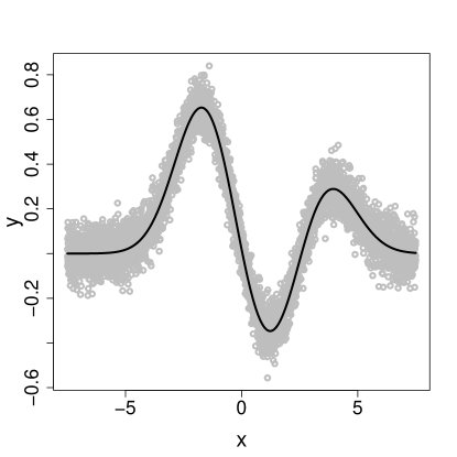
Figure 1: The function $f$ evaluated on $[-7.5,7.5]$ (black) and one realisation of the noisy data $y=f(x)+\varepsilon$ (grey).

In condition (D1) we set $\sigma^{2}_{x}=\Sigma=4$. For the matrix $V^{2}=[\tau_{|i-j|}]_{i,j=1}^{n}\in{\mathbb{R}}^{n\times n}$ we choose three different structures for $n\in\{200,400,1000\}$. In the first setting $\tau_{h}=\mathbb{I}(h=0)$, which corresponds to independent data. The second setting with $\tau_{h}=0.9^{-h}$ implies an autoregressive process of order one. Finally, the third setting with $\tau_{h}=(1+h)^{-q}$, $q=1/4$, $h=0,\dots,n-1$ leads to the long range dependent case.

In a Monte Carlo simulation with $M=1000$ repetitions the time series $\{X_{t}^{(j)}\}_{t=1}^{n}$ are generated via $X^{(j)}=VN^{(j)}$ with $N^{(j)}\sim\mathcal{N}_{n}(0,\sigma^{2}I_{n})$, $j=1,\dots,M$, where $I_{n}$ is the $n\times n$-dimensional identity matrix.

The residuals $\varepsilon_{1}^{(j)},\dots,\varepsilon_{n}^{(j)}$ are generated as independent standard normally distributed random variables and independent of $\{X_{t}^{(j)}\}_{t=1}^{n}$ . The response is defined as $y_{t}^{(j)}=f(X_{t}^{(j)})+\eta\,\varepsilon_{t}^{(j)}$, $t=1,\dots,n$, $j=1,\dots,M$, with $\eta=1/16$.

The kernel partial least squares and kernel conjugate gradient algorithms are run for each sample $\{(X_{t}^{(j)},y_{t}^{(j)})^{\mathrm{\scriptscriptstyle T}}\}_{t=1}^{n}$, $j=1,\dots,M$, with a maximum of $40$ iteration steps. We denote the estimated coefficients with $\widehat{\alpha}_{1}^{(j,m)},\dots,\widehat{\alpha}_{40}^{(j,m)}$, $j=1,\dots,M$, with $m=CG$ meaning that the kernel conjugate gradient algorithm was employed and $m=PLS$ that kernel partial least squares was used to estimate $\alpha_{1},\dots,\alpha_{n}$.

The squared error in the $\mathcal{L}^{2}\left(\mathrm{P}^{X}\right)$-norm is calculated via

$$\widehat{e}_{n,\tau}^{(j,m)}=\min\limits_{a=1,\dots,40}\left[\frac{1}{\sqrt{2\pi\sigma_{x}^{2}}}\int\limits_{-\infty}^{\infty}\left\{f_{\widehat{\alpha}_{a}^{(j,m)}}(x)-f(x)\right\}^{2}\exp\left(-\frac{1}{2\sigma_{x}^{2}}x^{2}\right)\mathrm{d}x\right],$$

for $j=1,\dots,M$, $n=200,400,\dots,1000$ and $m\in\{CG,PLS\}$.

The results of the Monte-Carlo simulations are depicted in the boxplots of Figure 2.

Figure 2: Boxplots of the $\mathcal{L}^{2}\left(\mathrm{P}^{X}\right)$-errors $\{\widehat{e}_{n,\tau}^{(j,m)}\}_{j=1}^{M}$ of kernel partial least squares (left side of each panel) and kernel conjugate gradient (right side of each panel) for different autocovariance functions $\tau$ and $n=200,400,1000$. On the left is $\tau_{h}=\mathbb{I}(h=0)$, in the middle $\tau_{h}=0.9^{-h}$ and on the right $\tau_{h}=(h+1)^{-1/4}$.

For kernel partial least squares (left panels) one observes that independent and autoregressive dependent data have roughly the same convergence rates, although the latter have a somewhat higher error. In contrast, the long range dependent data show slower convergence with the larger interquartile range, supporting the theoretical results of Corollary 3.

The $\mathcal{L}^{2}\left(\mathrm{P}^{X}\right)$-error of kernel conjugate gradient estimators is generally slightly higher than that of kernel partial least squares. Nonetheless, both of them have a similar behaviour.

We also investigated the the stopping indices $a=1,\dots,40$ for which the errors $\widehat{e}_{n,\tau}^{(j,m)}$ were attained. These are shown in Figure 3 for independent and identically distributed data.

Figure 3: Boxplots of the optimal indices $a\in\{1,\dots,40\}$ for which the $\mathcal{L}^{2}\left(\mathrm{P}^{X}\right)$-errors $\{\widehat{e}_{n,\tau}^{(j,m)}\}_{j=1}^{M}$ were attained. Kernel partial least squares is on the left of each panel and kernel conjugate gradient on the right. On the left is $n=200$, on the right $n=1000$. The data were assumed to be independent and identically distributed.

It can be seen that the optimal indices for both algorithms have a rather similar behaviour. Kernel conjugate gradient stops slightly later, but overall the differences seem negligible.

Figure 4 shows the mean (over $j$) of the estimated $\mathcal{L}^{2}\left(\mathrm{P}^{X}\right)$ errors $\{\widehat{e}_{n,\tau}^{(j,m)}\}_{j=1}^{M}$ for different $n$, $\tau$ and $m\in\{CG,PLS\}$. The errors were multiplied by $n/\log(n)$ to illustrate the convergence rates. According to Proposition 2 and Corollary 3 (ii) we expect the rates for the independent and autoregressive cases to be $n^{-1}\log(n)$, which is verified by the fact that the solid black and grey lines are roughly constant. For the long range dependent case we expect worse convergence rates which are also illustrated by the divergence of the dashed black line.

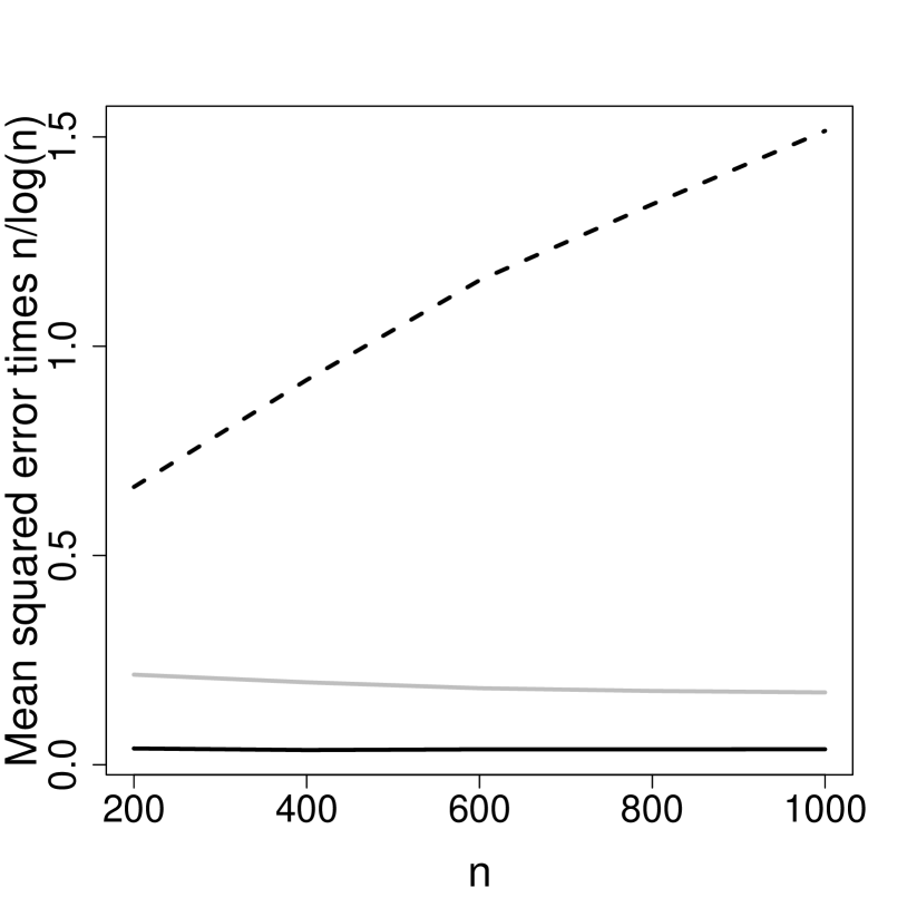
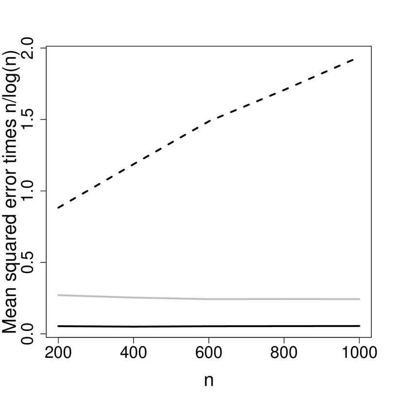
Figure 4: Mean of the $\mathcal{L}^{2}\left(\mathrm{P}^{X}\right)$-errors $\{\widehat{e}_{n,\tau}^{(j,m)}\}_{j=1}^{M}$ of kernel partial least squares (left) and kernel conjugate gradient (right) for $n=200,400,\dots,1000$ multiplied by $n/\log(n)$. The solid black line is for $\tau_{h}=\mathbb{I}(h=0)$, the grey line for $\tau_{h}=0.9^{-h}$ and the dashed black line for $\tau_{h}=(h+1)^{-1/4}$.

7 Application to Molecular Dynamics Simulations

The collective motions of protein atoms are responsible for its biological function and molecular dynamics simulations is a popular tool to explore this (Henzler-Wildman and Kern,, 2007).

Typically, the $p\in{\mathbb{N}}$ backbone atoms of a protein are considered for the analysis with the relevant dynamics happening in time frames of nanoseconds. Although the dynamics are available exactly, the high dimensionality of the data and large number of observations can be cumbersome for regression analysis, e.g., due to the high collinearity in the columns of the covariates matrix. Many function-dynamic relationships are also non-linear (Hub and de Groot,, 2009). A further complication is the fact that the motions of different backbone atoms are highly correlated, making additive non-parametric models for the target function $f^{\ast}$ less suitable.

We consider T4 Lysozyme (T4L) of the bacteriophage T4, a protein responsible for the hydrolisis of 1,4-beta-linkages in peptidoglycans and chitodextrins from bacterial cell walls. The number of available observations is $n=4601$ and T4L consists of $p=486$ backbone atoms.

Denote with $A_{t,i}\in{\mathbb{R}}^{3}$ the $i$-th atom, $i=1,\dots,p$, at time $t=1,\dots,n$ and $c_{i}\in{\mathbb{R}}^{3}$ the $i$-th atom in the (apo) crystal structure of T4L. A usual representation of the protein in a regression setting is the Cartesian one, i.e., we take as the covariate $X_{t}=(A_{1,t}^{\mathrm{\scriptscriptstyle T}},\dots,A^{\mathrm{\scriptscriptstyle T}}_{p,t})^{\mathrm{\scriptscriptstyle T}}$, $t=1,\dots,n$, see Brooks and Karplus, (1983). The functional quantity to predict is the root mean square deviation of the protein configuration $X_{t}$ at time $t=1,\dots,n$ from the (apo) crystal structure $C=(c_{1}^{\mathrm{\scriptscriptstyle T}},\dots,c_{d}^{\mathrm{\scriptscriptstyle T}})^{\mathrm{\scriptscriptstyle T}}$, i.e.,

$$y_{t}=\left\{p^{-1}\sum\limits_{i=1}^{p}\|X_{i,t}-C_{i}\|^{2}\right\}^{1/2}.$$

This nonlinear function was previously considered in Hub and de Groot, (2009), where it was established that linear models are insufficient for the prediction.

Figure 5 shows the time series corresponding to $X_{t,1}$ (i.e., the first coordinate of the first atom of T4L) on the left and the functional quantity $y_{t}$ on the right. These plots reveal certain persistent dependence over time.

Figure 5: Time series of $X_{t,1}$, i.e., the first coordinate of the first atom T4L consists of (left) and the root mean squared deviation $y_{t}$ between the protein configuration at time $t$ and the (apo) crystal structure.

Fitting autoregressive moving average models of order $(3,2)$ ($ARMA(3,2)$) to $y_{t}$ and $ARMA(5,2)$ to $X_{t,1}$ shows that the smallest root of their respective characteristic polynomial is close to one ($1.009$ for $y_{t}$ and $1.003$ for $X_{t,1}$), highlighting that we are on the border of stationarity, see, e.g., Brockwell and Davis, (1991).

Figure 6 depicts the autocorrelation functions of $X_{t,1}$ and $y_{t}$, the theoretical autocorrelation function of the corresponding autoregressive moving average process and $\rho_{h}\propto(h+1)^{-q}$ for $q=0.134$ for $X_{t,1}$ and $q=0.066$ for $y_{t}$. The latter, as highlighted in Section 4, is an autocorrelation function for a stationary long range dependent process.

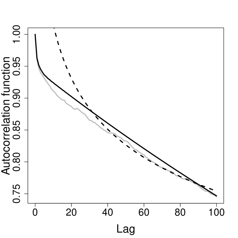
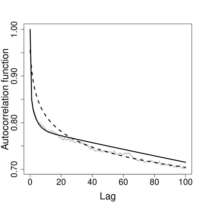
Figure 6: Autocorrelation plots of $X_{t,1}$ (left) and $y_{t}$ (right). The estimated autocorrelation function is grey, the theoretical one of a fitted $ARMA(3,2)$ process is solid black and $\rho_{h}\propto(h+1)^{-q}$ for a suitable choice of $q>0$ is dashed black.

These plots suggest that $X_{t,1}$ and $y_{t}$ follow some long-range stationary process.

We apply kernel partial least squares to this data set with the Gaussian kernel $k(x,y)=\exp(-l\|x-y\|^{2})$, $x,y\in{\mathbb{R}}^{3p}$, $l>0$. The function $f$ we aim to estimate is a distance between protein configurations, so using a distance based kernel seems reasonable. Moreover, we also investigated the impact of other bounded kernels such as triangular and Epanechnikov and obtained similar results. The first $25\%$ of the data form a training set to calculate the kernel partial least squares estimator and the remaining data are used for testing.

The parameter $l>0$ is calculated via cross validation on the training set. In our evaluation we obtained $l=0.0189$.

Figure 7 compares the observed response in the test set with the prediction on the test set obtained by kernel partial least squares, kernel principal component regression and linear partial least squares.

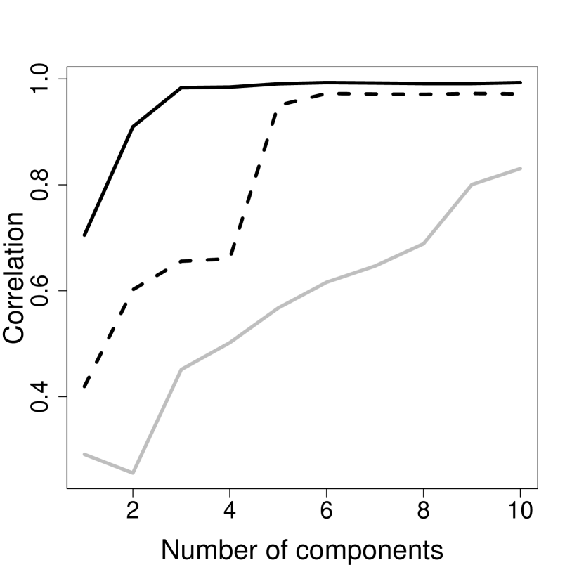
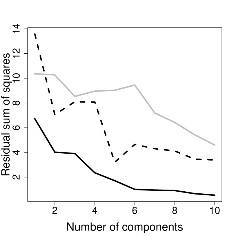
Figure 7: Correlation (left) and residual sum of squares (right) between predicted values and the observed response on the test set depending on the number of used components for kernel partial least squares (solid black), partial least squares (grey) and kernel principal component regression (dashed black).

Apparently, kernel partial least squares show the best performance and the kernel principal components algorithm is able to achieve comparable prediction with more components only. Obviously, linear partial least squares can not cope with the non-linearity of the problem.

This application highlights that kernel partial least squares still delivers a robust prediction even when the dependence in the data is more persistent, if enough observations are available.

Appendix A Proofs

A.1 Proof of Theorem 1

The proof of Theorem 1 makes use of the connection between the partial least squares and the conjugate gradient algorithm. This section is structured as follows: First we will introduce the link between kernel partial least squares and kernel conjugate gradient. We will state some key facts about orthogonal polynomials and their relationship to the algorithm in Lemma 1. Then the consistency of kernel partial least squares is shown with the help of three error bounds that are obtained in Lemmas 3 – 5.

With a slight abuse of notation we define $f_{i}=f_{\widehat{\alpha}_{i}}$ for $i=1,\dots,n$. We consider the kernel partial least squares algorithm as an optimization problem

$$f_{i}=\arg\min\limits_{g\in\mathcal{K}_{i}(S_{n},T_{n}^{\ast}y)}\|y-T_{n}g\|^{2},\leavevmode\nobreak\ \leavevmode\nobreak\ i=1,\dots,n.$$ (8)

This is the conjugate gradient algorithm CGNE discussed in chapter 2.2 of Hanke, (1995).

A.1.1 Orthogonal polynomials and some notation

Denote with $\mathcal{P}_{i}$ the set of polynomials of degree at most $i=0,\dots,n$. For functions $\psi,\phi:{\mathbb{R}}\rightarrow{\mathbb{R}}$ and $r\in{\mathbb{N}}_{0}$ define the inner products $[\psi,\phi]_{r}=\langle\psi(S_{n})T_{n}^{\ast}y,S_{n}^{r}\phi(S_{n})T_{n}^{\ast}y\rangle_{\mathcal{H}}$. From the definition of the Krylov space it is immediate that every element $v\in\mathcal{K}_{i}(S_{n},T_{n}^{\ast}y)$, $i=1,\dots,n$, can be represented by a polynomial $q\in\mathcal{P}_{i-1}$ via $v=q(S_{n})T_{n}^{\ast}y$.

The following discussion is based on Hanke, (1995), chapter 2. There exist two sequences of polynomials $\{p_{i}\}_{i=0}^{n},\{q_{i}\}_{i=0}^{n}\subset\mathcal{P}_{i}$, such that $f_{i}=q_{i-1}(S_{n})T_{n}^{\ast}y$ with $q_{-1}=0$ and $T_{n}^{\ast}y-S_{n}f_{i}=p_{i}(S_{n})T_{n}^{\ast}y$. Both sequences are connected by the equation $p_{i}(x)=1-xq_{i-1}(x)$, $x\in{\mathbb{R}}$, and the polynomials $\{p_{i}\}_{i=0}^{n}$ are orthogonal with respect to $[\cdot,\cdot]_{0}$.

We will also consider other sequences of polynomials, namely $\{q_{i}^{[r]}\}_{i=0}^{n},\{p_{i}^{[r]}\}_{i=0}^{n}\subset\mathcal{P}_{i}$, $q_{-1}^{[r]}=0$, such that $p_{i}^{[r]}(x)=1-xq_{i-1}^{[r]}(x)$, $x\in{\mathbb{R}}$, and the sequence $\{p_{i}^{[r]}\}_{i=0}^{n}$ is orthogonal with respect to $[\cdot,\cdot]_{r}$. This yields for every $r\in{\mathbb{N}}_{0}$ a separate conjugate gradient algorithm with solution $f_{i}^{[r]}=q_{i-1}^{[r]}(S_{n})T_{n}^{\ast}y\in\mathcal{K}_{i}(S_{n},T_{n}^{\ast}y)$ and residuals $T_{n}^{\ast}y-S_{n}f_{i}^{[r]}=p_{i}^{[r]}(S_{n})T_{n}^{\ast}y$, $i=1,\dots,n$. The $p_{i}^{[r]}$, $i=0,\dots,n$, $r\in{\mathbb{N}}_{0}$, are called residual polynomials.

As $S_{n}$ is self-adjoint, positive semi-definite and the kernel is bounded by $\kappa$ we know that its spectrum is a subset of $[0,\kappa]$, see Caponnetto and de Vito, (2007). This also implies that $\max\{\|S\|_{\mathcal{L}},\|S_{n}\|_{\mathcal{L}}\}\leq\kappa$, with $\|\cdot\|_{\mathcal{L}}$ denoting the operator norm. The $i$ distinct roots of $p_{i}^{[r]}$ will be denoted by $0<x_{1,i}^{[r]}<\dots x_{i,i}^{[r]}<\kappa$, $i=1,\dots,n$.

We will summarize some key facts about the orthogonal polynomials in the next lemma.

Lemma 1

Let $r,s\in{\mathbb{N}}_{0}$ and $i=1,\dots,n$. Then we have:

• The roots of consecutive orthogonal polynomials interlace, i.e., for $j=1,\dots,i$ it holds

  $$0<x_{j,i+1}^{[r]}<x_{j,i}^{[r]}<x_{j,i}^{[r+1]}<x_{j+1,i+1}^{[r]}<x_{j+1,i}^{[r]}<\dots<x_{i,i}^{[r+1]}<x_{i+1,i+1}^{[r]}<\kappa,$$

• the optimality property $[p_{i}^{[1]},p_{i}^{[1]}]_{0}^{1/2}=\|T_{n}^{\ast}y-S_{n}f_{i}^{[1]}\|_{\mathcal{H}}\leq\|T_{n}^{\ast}y-S_{n}h\|_{\mathcal{H}}$ holds for all $h\in\mathcal{K}_{i}(S_{n},T_{n}^{\ast}y)$,

• on $x\in[0,x_{1,i}^{[r]}]$ it holds $0\leq p_{i}^{[r]}(x)\leq 1$ and $q_{i}^{[r]}(x)\leq\left|\left(p_{i}^{[r]}\right)^{\prime}(0)\right|$,

• $p_{n}^{[r]}=p_{n}^{[s]},$

• $\left(p_{i}^{[r]}\right)^{\prime}(0)=-\sum_{j=1}^{i}\left(x_{j,i}^{[r]}\right)^{-1}$,

• for $r\geq 1$ define $\phi_{i}(x)=p_{i}^{[r]}(x)\left(x_{1,i}^{[r]}\right)^{1/2}\left(x_{1,i}^{[r]}-x\right)^{-1/2}$, $x\in[0,x_{1,i}^{[r]}]$, $i=1,\dots,n$. Then it holds for $u\geq 0$ that $x^{u}\phi^{2}_{i}(x)\leq u^{u}\left|\left(p_{i}^{[r]}\right)^{\prime}(0)\right|^{-u}$ with the convention $0^{0}=1$.

Proof: (i) See Hanke, (1995), Corollary 2.7.

(ii) See Hanke, (1995), Proposition 2.1.

(iii) Due to part (i) we know that all $i$ roots of the polynomial $p_{i}^{[r]}$ are contained in $(0,\kappa)$. Furthermore $p_{i}^{[r]}(0)=1-0q_{i}^{[r]}=1$. Thus $p_{i}^{[r]}$ is convex and falling in $[0,x_{1,i}^{[r]}]$ and the first assertion follows.

Because of the convexity of $p_{i}^{[r]}$ on $[0,x_{1,i}^{[r]}]$ we get $q_{i}^{[r]}(x)=x^{-1}\{1-p_{i}^{[r]}(x)\}\leq\left|\left(p_{i}^{[r]}\right)^{\prime}(0)\right|$.

(iv) See the discussion in Hanke, (1995) preceding Proposition 2.1 and use the facts that $T_{n}^{\ast}y\in\mathrm{range}(S_{n})$ and $S_{n}$ is an operator of rank $n$.

(v) Write $p_{i}^{[r]}(x)=\prod_{j=1}^{i}(1-x/x_{j,i}^{[r]})$, $x\in[0,\kappa]$, and the result is immediate.

(vi) See equation (3.10) in Hanke, (1995). $\square$

We denote for $x\geq 0$ by $P_{x}$ the orthogonal projection operator on the eigenspace corresponding to the eigenvalues of $S_{n}$ that are smaller or equal $x$ and $P_{x}^{\perp}=I_{\mathcal{H}}-P_{x}$ with $I_{\mathcal{H}}:\mathcal{H}\rightarrow\mathcal{H}$ being the identity operator.

A.1.2 Preparation for the proof

An important technical result that will be useful in the upcoming proof is

Lemma 2

Let $B,C:\mathcal{H}\rightarrow\mathcal{H}$ be two positive semi-definite, self-adjoint operators with $\max\{\|B\|_{\mathcal{L}},\|C\|_{\mathcal{L}}\}\leq\kappa$. Then it holds for any $r\geq 0$ with $\zeta=\max\{r-1,0\}$

$$\|B^{r}-C^{r}\|_{\mathcal{L}}\leq(\zeta+1)\kappa^{\zeta}\|B-C\|_{\mathcal{L}}^{r-\zeta}.$$

Proof: See Blanchard and Krämer, 2010b , Lemma A.6. $\square$

For the remainder of the proof we assume that we are on the set where it holds with probability at least $1-\nu$, $\nu\in(0,1]$, that $\|S_{n}-S\|_{\mathcal{L}}\leq C_{\delta}(\nu)\gamma_{n}$ and $\|T_{n}^{\ast}y-Sf\|\leq C_{\epsilon}(\nu)\gamma_{n}$ for a sequence $\{\gamma_{n}\}_{n}$ converging to zero and constants $C_{\delta}=C_{\delta}(\nu),C_{\epsilon}=C_{\epsilon}(\nu)>0$.

With Lemma 2.4 in Hanke, (1995) we see that the stopping iteration (5) can also be expressed as

$${a^{\ast}}=\min\left\{1\leq a\leq n:\|S_{n}f_{a}^{[1]}-T_{n}^{\ast}y\|_{\mathcal{H}}\leq C\gamma_{n}\right\},$$ (9)

i.e., we stop the kernel partial least squares algorithm when a discrepancy principle for $f_{a}^{[1]}$ holds.

It is easy to see that from (S) it follows for $r\geq 1/2$ that

1. There exist $\mu\geq 0$, $R>0$ and $u\in\mathcal{H}$ such that $f=S^{\mu}u$ and $\|u\|_{\mathcal{H}}\leq R$.

This condition is known as the Hölder source condition with $\mu=r-1/2$.

Recall that $\mathcal{H}\subseteq\mathcal{L}^{2}\left(\mathrm{P}^{X}\right)$ and $T:\mathcal{H}\rightarrow\mathcal{L}^{2}\left(\mathrm{P}^{X}\right)$ is the change of space operator. Using the fact that $T$, $T^{\ast}$ are adjoint operators, $f_{a^{\ast}}=Tf_{a^{\ast}}$ and $f^{\ast}=Tf$ for $r\geq 1/2$ we see

$$\|f_{a^{\ast}}-f^{\ast}\|_{2}=\|T(f_{a^{\ast}}-f)\|_{2}=\langle S(f_{a^{\ast}}-f),f_{a^{\ast}}-f\rangle_{\mathcal{H}}=\|S^{1/2}(f_{a^{\ast}}-f)\|_{\mathcal{H}}.$$

An application of Lemma 2 yields

$$\|f_{a^{\ast}}-f^{\ast}\|_{2}=\|S^{1/2}(f_{a^{\ast}}-f)\|_{\mathcal{H}}\leq\|S^{1/2}(f_{a^{\ast}}-f_{{a^{\ast}}}^{[1]})\|_{\mathcal{H}}+\|S^{1/2}(f_{{a^{\ast}}}^{[1]}-f)\|_{\mathcal{H}}$$

$$\leq C_{\delta}^{1/2}\gamma_{n}^{1/2}\left(\|f_{a^{\ast}}-f_{{a^{\ast}}}^{[1]}\|_{\mathcal{H}}+\|f_{{a^{\ast}}}^{[1]}-f\|_{\mathcal{H}}\right)+\|S_{n}^{1/2}(f_{a^{\ast}}-f_{{a^{\ast}}}^{[1]})\|_{\mathcal{H}}+\|S_{n}^{1/2}(f_{{a^{\ast}}}^{[1]}-f)\|_{\mathcal{H}}.$$ (10)

The following lemmas will deal with bounding the quantities in (10).

Lemma 3

Assume $C_{x}\in(0,1]$ such that $x_{\ast}=(C_{x}\gamma_{n})^{1/(\mu+1)}<x_{1,{a^{\ast}}-1}^{[1]}$ and $C>C_{\epsilon}+C_{x}R+C_{\delta}(\mu+1)\kappa^{\mu}R$. Under the conditions of the theorem it holds $\mu\geq 0$

$$\|f_{a^{\ast}}-f_{{a^{\ast}}}^{[1]}\|_{\mathcal{H}} \leq\gamma^{\mu/(\mu+1)}_{n}\frac{C}{C_{x}^{1/(\mu+1)}\left[1-C^{-1}\{C_{\epsilon}+C_{x}R+C_{\delta}(\mu+1)\kappa^{\mu}R\}\right]^{2}}$$

$$\|S_{n}^{1/2}(f_{a^{\ast}}-f_{{a^{\ast}}}^{[1]})\|_{\mathcal{H}} \leq\gamma^{(2\mu+1)/(2\mu+2)}_{n}\frac{C}{C_{x}^{1/(2\mu+2)}\left[1-C^{-1}\{C_{\epsilon}+C_{x}R+C_{\delta}(\mu+1)\kappa^{\mu}R\}\right]}.$$

Proof: If the inner products $[\cdot,\cdot]_{0}$ and $[\cdot,\cdot]_{1}$ are the same the proof is done because both polynomial sequences are identical.

We now observe that we have for ${a^{\ast}}=n$ due to Lemma 1 (iv) $q_{n-1}(x)-q_{n-1}^{[1]}(x)=x^{-1}\{p_{n}^{[1]}(x)-p_{n}(x)\}=0$, i.e., $\|f_{{a^{\ast}}}-f_{{a^{\ast}}}^{[1]}\|_{\mathcal{H}}=0$ and $\|S_{n}^{1/2}(f_{{a^{\ast}}}-f_{{a^{\ast}}}^{[1]})\|_{\mathcal{H}}=0$ and the proof is done.

If the inner products differ and we have $0<{a^{\ast}}<n$ it holds $f_{a^{\ast}}\neq f_{{a^{\ast}}}^{[1]}$.

Proposition 2.8 in Hanke, (1995) can now be applied for $0<{a^{\ast}}<n$ and yields $q_{{a^{\ast}}-1}(x)-q_{{a^{\ast}}-1}^{[1]}(x)=x^{-1}\{p_{{a^{\ast}}}^{[1]}(x)-p_{{a^{\ast}}}(x)\}=\theta_{{a^{\ast}}}p_{{a^{\ast}}-1}^{[2]}(x)$, $x\geq 0$, with $\theta_{{a^{\ast}}}=(p_{{a^{\ast}}}^{[1]})^{\prime}(0)-(p_{{a^{\ast}}}^{[0]})^{\prime}(0)>0$. We get $f_{a^{\ast}}-f_{{a^{\ast}}}^{[1]}=q_{{a^{\ast}}-1}(S_{n})T_{n}^{\ast}y-q_{{a^{\ast}}-1}^{[1]}(S_{n})T_{n}^{\ast}y=\theta_{{a^{\ast}}}p_{{a^{\ast}}-1}^{[2]}(S_{n})T_{n}^{\ast}y$.

Proposition 2.9 in Hanke, (1995) yields $\theta_{{a^{\ast}}}=\left[p_{{a^{\ast}}-1}^{[2]},p_{{a^{\ast}}-1}^{[2]}\right]_{1}^{-1}\left[p_{{a^{\ast}}}^{[1]},p_{{a^{\ast}}}^{[1]}\right]_{0}$. The optimality property of $f_{{a^{\ast}}}^{[1]}$ in Lemma 1 (ii) shows that

$$\|T_{n}^{\ast}y-S_{n}f_{{a^{\ast}}}^{[1]}\|_{\mathcal{H}}=\|p_{{a^{\ast}}}^{[1]}(S_{n})T_{n}^{\ast}y\|_{\mathcal{H}}=\left[p_{{a^{\ast}}}^{[1]},p_{{a^{\ast}}}^{[1]}\right]_{0}^{1/2}\leq\left[p_{{a^{\ast}}-1}^{[2]},p_{{a^{\ast}}-1}^{[2]}\right]_{0}^{1/2}.$$ (11)

Combining these results yields

$$\|f_{a^{\ast}}-f_{{a^{\ast}}}^{[1]}\|_{\mathcal{H}}=\frac{\left[p_{{a^{\ast}}}^{[1]},p_{{a^{\ast}}}^{[1]}\right]_{0}}{\left[p_{{a^{\ast}}-1}^{[2]},p_{{a^{\ast}}-1}^{[2]}\right]_{1}}\left[p_{{a^{\ast}}-1}^{[2]},p_{{a^{\ast}}-1}^{[2]}\right]_{0}^{1/2}\leq\frac{\left[p_{{a^{\ast}}-1}^{[2]},p_{{a^{\ast}}-1}^{[2]}\right]_{0}}{\left[p_{{a^{\ast}}-1}^{[2]},p_{{a^{\ast}}-1}^{[2]}\right]_{1}}\|p_{{a^{\ast}}}^{[1]}(S_{n})T_{n}^{\ast}y\|_{\mathcal{H}}.$$ (12)

Recall that $x_{1,{a^{\ast}}-1}^{[2]}$ denotes the first root of $p_{{a^{\ast}}-1}^{[2]}$. It holds for any $0\leq x\leq x_{1,{a^{\ast}}-1}^{[2]}$ that $0\leq p_{{a^{\ast}}-1}^{[2]}(x)\leq 1$, see Lemma 1 (iii), and thus

$$\left[p_{{a^{\ast}}-1}^{[2]},p_{{a^{\ast}}-1}^{[2]}\right]_{0}^{1/2} \leq\|P_{x}p_{{a^{\ast}}-1}^{[2]}(S_{n})\{T_{n}^{\ast}y-Sf+Sf\}\|_{\mathcal{H}}+\|P_{x}^{\perp}p_{{a^{\ast}}-1}^{[2]}(S_{n})T_{n}^{\ast}y\|_{\mathcal{H}}$$

$$\leq C_{\epsilon}\gamma_{n}+\|P_{x}p_{{a^{\ast}}-1}^{[2]}(S_{n})S^{\mu+1}u\|_{\mathcal{H}}+x^{-1/2}\|P_{x}^{\perp}S_{n}^{1/2}p_{{a^{\ast}}-1}^{[2]}(S_{n})T_{n}^{\ast}y\|_{\mathcal{H}}$$

$$\leq C_{\epsilon}\gamma_{n}+x^{\mu+1}R+\|P_{x}p_{{a^{\ast}}-1}^{[2]}(S^{\mu+1}-S_{n}^{\mu+1})u\|_{\mathcal{H}}+x^{-1/2}\left[p_{{a^{\ast}}-1}^{[2]},p_{{a^{\ast}}-1}^{[2]}\right]_{1}^{1/2}.$$

In the second inequality (SH) with $\mu\geq 0$ was applied.

By assumption $x_{\ast}=(C_{x}\gamma)^{1/(\mu+1)}\leq x_{1,{a^{\ast}}-1}^{[1]}<x_{1,{a^{\ast}}-1}^{[2]}$ due to the interlacing property of the roots of the polynomials $p_{i}^{[r]}$, $i=1,\dots,n$, $r\in{\mathbb{N}}_{0}$, see Lemma 1 (i).

Using Lemma 2 we get $\|S^{\mu+1}-S_{n}^{\mu+1}\|_{\mathcal{L}}\leq(\mu+1)\kappa^{\mu}C_{\delta}\gamma_{n}$ and setting $x=x_{\ast}$ we get

$$\left[p_{{a^{\ast}}-1}^{[2]},p_{{a^{\ast}}-1}^{[2]}\right]_{0}^{1/2} \leq C_{\epsilon}\gamma_{n}+x_{\ast}^{\mu+1}R+C_{\delta}\gamma_{n}(\mu+1)\kappa^{\mu}R+x_{\ast}^{-1/2}\left[p_{{a^{\ast}}-1}^{[2]},p_{{a^{\ast}}-1}^{[2]}\right]_{1}^{1/2}$$

$$=\gamma_{n}\left\{C_{\epsilon}+C_{x}R+C_{\delta}(\mu+1)\kappa^{\mu}R\right\}+x_{\ast}^{-1/2}\left[p_{{a^{\ast}}-1}^{[2]},p_{{a^{\ast}}-1}^{[2]}\right]_{1}^{1/2}.$$ (13)

Due to (9) and (11) we have additionally $C\gamma_{n}\leq\|S_{n}f_{{a^{\ast}}-1}^{[1]}-T_{n}^{\ast}y\|_{\mathcal{H}}=\|p_{{a^{\ast}}-1}^{[1]}(S_{n})T_{n}^{\ast}y\|_{\mathcal{H}}\leq\left[p_{{a^{\ast}}-1}^{[2]},p_{{a^{\ast}}-1}^{[2]}\right]_{0}^{1/2}.$

Plugging this into (13) yields

$$\left[p_{{a^{\ast}}-1}^{[2]},p_{{a^{\ast}}-1}^{[2]}\right]_{0}^{1/2}\leq C^{-1}\{C_{\epsilon}+C_{x}R+C_{\delta}(\mu+1)\kappa^{\mu}R\}\left[p_{{a^{\ast}}-1}^{[2]},p_{{a^{\ast}}-1}^{[2]}\right]_{0}^{1/2}+x_{\ast}^{-1/2}\left[p_{{a^{\ast}}-1}^{[2]},p_{{a^{\ast}}-1}^{[2]}\right]_{1}^{1/2},$$

or equivalently with $x_{\ast}=(C_{x}\gamma_{n})^{1/(\mu+1)}$

$$\left[p_{{a^{\ast}}-1}^{[2]},p_{{a^{\ast}}-1}^{[2]}\right]_{0}^{1/2}\leq\gamma^{-1/(2\mu+2)}_{n}\frac{\left[p_{{a^{\ast}}-1}^{[2]},p_{{a^{\ast}}-1}^{[2]}\right]_{1}^{1/2}}{C_{x}^{1/(2\mu+2)}\left[1-C^{-1}\{C_{\epsilon}+C_{x}R+C_{\delta}(\mu+1)\kappa^{\mu}R\}\right]},$$ (14)

where by assumption $C>C_{\epsilon}+C_{x}R+C_{\delta}(\mu+1)\kappa^{\mu}R$ and $x_{\ast}=(C_{x}\gamma)^{1/(\mu+1)}$.

Combining (12), (14) and $\|p_{{a^{\ast}}}^{[1]}(S_{n})T_{n}^{\ast}y\|_{\mathcal{H}}\leq C\gamma_{n}$ due to the stopping index (9) yields

$$\|f_{a^{\ast}}-f_{{a^{\ast}}}^{[1]}\|_{\mathcal{H}} \leq\gamma^{-1/(\mu+1)}_{n}\frac{\|p_{{a^{\ast}}}^{[1]}(S_{n})T_{n}^{\ast}y\|_{\mathcal{H}}}{C_{x}^{1/(\mu+1)}\left[1-C^{-1}\{C_{\epsilon}+C_{x}R+C_{\delta}(\mu+1)\kappa^{\mu}R\}\right]^{2}}$$

$$\leq\gamma^{\mu/(\mu+1)}_{n}\frac{C}{C_{x}^{1/(\mu+1)}\left[1-C^{-1}\{C_{\epsilon}+C_{x}R+C_{\delta}(\mu+1)\kappa^{\mu}R\}\right]^{2}}.$$

For the second part of the proof we derive in the same way as (12)

$$\|S_{n}^{1/2}(f_{a^{\ast}}-f_{{a^{\ast}}}^{[1]})\|_{\mathcal{H}}\leq\frac{\left[p_{{a^{\ast}}-1}^{[2]},p_{{a^{\ast}}-1}^{[2]}\right]_{0}^{1/2}}{\left[p_{{a^{\ast}}-1}^{[2]},p_{{a^{\ast}}-1}^{[2]}\right]_{1}^{1/2}}\|p_{{a^{\ast}}}^{[1]}(S_{n})T_{n}^{\ast}y\|_{\mathcal{H}}.$$

Using (14) and $\|p_{{a^{\ast}}}^{[1]}(S_{n})T_{n}^{\ast}y\|_{\mathcal{H}}\leq C\gamma_{n}$ gives

$$\|S_{n}^{1/2}(f_{a^{\ast}}-f_{{a^{\ast}}}^{[1]})\|_{\mathcal{H}}\leq\gamma^{(2\mu+1)/(2\mu+2)}_{n}\frac{C}{C_{x}^{1/(2\mu+2)}\left[1-C^{-1}\{C_{\epsilon}+C_{x}R+C_{\delta}(\mu+1)\kappa^{\mu}R\}\right]},$$

finishing the proof. $\square$

Lemma 4

For any $i=1,\dots,n$ and any $0<x\leq x_{1,i}^{[1]}$ we have under the conditions of the theorem for $\mu\geq 1$

$$\|f-f_{i}^{[1]}\|_{\mathcal{H}} \leq R\left\{x^{\mu}+C_{\delta}\mu\kappa^{\mu-1}\gamma_{n}\right\}+x^{-1}\left\{\|S_{n}f_{i}^{[1]}-T_{n}^{\ast}y\|_{\mathcal{H}}+(C_{\epsilon}+C_{\delta}\kappa^{\mu}R)\gamma_{n}\right\}$$

$$+(C_{\epsilon}+C_{\delta}\kappa^{\mu}R)\gamma_{n}|(p_{i}^{[1]})^{\prime}(0)|,$$

$$\|S_{n}^{1/2}(f-f_{i}^{[1]})\|_{\mathcal{H}} \leq R\left\{x^{\mu+1/2}+x^{1/2}C_{\delta}\mu\kappa^{\mu-1}\gamma_{n}\right\}$$

$$+x^{-1/2}\left\{\|S_{n}f_{i}^{[1]}-T_{n}^{\ast}y\|_{\mathcal{H}}+(C_{\epsilon}+C_{\delta}\kappa^{\mu}R)\gamma_{n}\right\}$$

$$+x^{1/2}(C_{\epsilon}+C_{\delta}\kappa^{\mu}R)\gamma_{n}|(p_{i}^{[1]})^{\prime}(0)|.$$

Proof: Denote $\bar{f}_{i}=q_{i-1}^{[1]}(S_{n})S_{n}f$ and consider

$$\|f-f_{i}^{[1]}\|_{\mathcal{H}}\leq\|P_{x}(f-\bar{f}_{i})\|_{\mathcal{H}}+\|P_{x}(\bar{f}_{i}-f_{i}^{[1]})\|_{\mathcal{H}}+\|P_{x}^{\perp}(f-f_{i}^{[1]})\|_{\mathcal{H}}.$$ (15)

The first term of (15) can be bound by an application of Lemma 2 and (SH) with $\mu\geq 1$

$$\|P_{x}(f-\bar{f}_{i})\|_{\mathcal{H}} =\|P_{x}\{I-q_{i-1}^{[1]}(S_{n})S_{n}\}f\|_{\mathcal{H}}=\|P_{x}p_{i}^{[1]}(S_{n})f\|_{\mathcal{H}}=\|P_{x}p_{i}^{[1]}(S_{n})S^{\mu}u\|_{\mathcal{H}}$$

$$\leq\|P_{x}p_{i}^{[1]}(S_{n})S_{n}^{\mu}u\|_{\mathcal{H}}+\|P_{x}p_{i}^{[1]}(S_{n})(S^{\mu}-S_{n}^{\mu})u\|_{\mathcal{H}}$$

$$\leq R\left\{x^{\mu}+C_{\delta}\mu\kappa^{\mu-1}\gamma_{n}\right\}.$$

In the last inequality we used that on $0\leq x\leq x_{1,i}^{[1]}$ we have $0\leq p_{i}^{[1]}(x)\leq 1$.

For the second term of (15) we use Lemma 1 (iii) $q_{i}^{[1]}(x)\leq|(p_{i}^{[1]})^{\prime}(0)|$ on $x\in[0,x_{1,i}^{[1]}]$. This yields

$$\|P_{x}(f_{i}^{[1]}-\bar{f}_{i})\|_{\mathcal{H}} =\|P_{x}q_{i}^{[1]}(S_{n})(S_{n}f-T_{n}^{\ast}y)\|_{\mathcal{H}}$$

$$\leq\|P_{x}q_{i}^{[1]}(S_{n})(Sf-T_{n}^{\ast}y)\|_{\mathcal{H}}+\|P_{x}q_{i}^{[1]}(S_{n})(S_{n}-S)f\|_{\mathcal{H}}$$

$$\leq(C_{\epsilon}+C_{\delta}\kappa^{\mu}R)\gamma_{n}\left|\left(p_{i}^{[1]}\right)^{\prime}(0)\right|.$$

Finally, we have

$$\|P_{x}^{\perp}(f-f_{i}^{[1]})\|_{\mathcal{H}} \leq x^{-1}\|P_{x}^{\perp}S_{n}(f-f_{i}^{[1]})\|_{\mathcal{H}}\ \leq x^{-1}\left\{\|S_{n}f_{i}^{[1]}-T_{n}^{\ast}y\|_{\mathcal{H}}+\|P_{x}(T_{n}^{\ast}y-S_{n}f)\|_{\mathcal{H}}\right\}$$

$$\leq x^{-1}\left\{\|S_{n}f_{i}^{[1]}-T_{n}^{\ast}y\|_{\mathcal{H}}+(C_{\epsilon}+C_{\delta}\kappa^{\mu}R)\gamma_{n}\right\}$$

and thus the first inequality is proven.

For the second inequality we use

$$\|S_{n}^{1/2}(f-f_{i}^{[1]})\|_{\mathcal{H}}\leq\|P_{x}S_{n}^{1/2}(f-\bar{f}_{i})\|_{\mathcal{H}}+\|P_{x}S_{n}^{1/2}(\bar{f}_{i}-f_{i}^{[1]})\|_{\mathcal{H}}+\|P_{x}^{\perp}S_{n}^{1/2}(f-f_{i}^{[1]})\|_{\mathcal{H}}.$$

In the same way as before we derive bounds for the three terms:

$$\|P_{x}S_{n}^{1/2}(f-\bar{f}_{i})\|_{\mathcal{H}} \leq x^{1/2}C_{\delta}\mu\kappa^{\mu-1}R\gamma_{n}+x^{\mu+1/2}R,$$

$$\|P_{x}S_{n}^{1/2}(\bar{f}_{i}-f_{i}^{[1]})\|_{\mathcal{H}} \leq x^{1/2}(C_{\epsilon}+C_{\delta}R\kappa^{\mu})\gamma_{n}\left|\left(p_{i}^{[1]}\right)^{\prime}(0)\right|,$$

$$\|P_{x}^{\perp}S_{n}^{1/2}(f-f_{i}^{[1]})\|_{\mathcal{H}} \leq x^{-1/2}\{\|S_{n}f_{i}^{[1]}-T_{n}^{\ast}y\|_{\mathcal{H}}+(C_{\epsilon}+C_{\delta}\kappa^{\mu}R)\gamma_{n}\},$$

completing the proof. $\square$

Lemma 5

Assume that $C_{x}\in(0,1]$ is such that $x_{\ast}=(C_{x}\gamma)^{1/(\mu+1)}<x_{1,{a^{\ast}}-1}^{[1]}$ and $C>C_{\epsilon}+C_{x}R+C_{\delta}(\mu+1)\kappa^{\mu}R$. Under the conditions of the theorem it holds for $\mu\geq 0$

$$\left|\left(p_{{a^{\ast}}}^{[1]}\right)^{\prime}(0)\right| \leq\gamma^{-1/(\mu+1)}_{n}\left[C_{x}^{-1/(\mu+1)}\left\{1-\frac{C_{\epsilon}+C_{x}R+C_{\delta}(\mu+1)\kappa^{\mu}R}{C}\right\}^{-2}\right.$$

$$+\left.\left\{\frac{(2\mu+2)^{\mu+1}R}{C-C_{\delta}(\mu+1)\kappa^{\mu}R+C_{\epsilon}}\right\}^{1/(\mu+1)}\right]$$

Proof: The proof is done in two steps by using the inequality $\left|\left(p_{{a^{\ast}}}^{[1]}\right)^{\prime}(0)\right|\leq\left|\left(p_{{a^{\ast}}-1}^{[1]}\right)^{\prime}(0)\right|+\left|\left(p_{{a^{\ast}}}^{[1]}\right)^{\prime}(0)-\left(p_{{a^{\ast}}-1}^{[1]}\right)^{\prime}(0)\right|$.

Consider first ${a^{\ast}}>1$.

We will bound $\|S_{n}f_{{a^{\ast}}-1}^{[1]}-T_{n}^{\ast}y\|_{\mathcal{H}}$ from above. Define $z=x_{1,{a^{\ast}}-1}^{[1]}$ and $\phi_{i}(x)=p_{i}^{[1]}(x)(z-x)^{-1/2}z^{1/2}$, $0\leq x\leq z$. Due to Lemma 1 (vi) it holds that $\sup_{0\leq x\leq z}x^{\nu}\phi_{{a^{\ast}}-1}^{2}(x)\leq\nu^{\nu}|(p_{{a^{\ast}}-1}^{[1]})^{\prime}(0)|^{-\nu}$, $\nu\geq 0$. The proof of Lemma 3.7 in Hanke, (1995) shows that

$$\left[p_{{a^{\ast}}-1}^{[1]},p_{{a^{\ast}}-1}^{[1]}\right]_{0}^{1/2}\leq\|P_{z}\phi_{{a^{\ast}}-1}(S_{n})T_{n}^{\ast}y\|_{\mathcal{H}}.$$

This yields with (SH)

$$\|S_{n}f_{{a^{\ast}}-1}^{[1]}-T_{n}^{\ast}y\|_{\mathcal{H}}=\left[p_{{a^{\ast}}-1}^{[1]},p_{{a^{\ast}}-1}^{[1]}\right]_{0}^{1/2}\leq\|P_{z}\phi_{{a^{\ast}}-1}(S_{n})T_{n}^{\ast}y\|_{\mathcal{H}}$$

$$\leq\|P_{z}\phi_{{a^{\ast}}-1}(S_{n})Sf\|_{\mathcal{H}}+\|P_{z}\phi_{{a^{\ast}}-1}(S_{n})(T_{n}^{\ast}y-Sf)\|_{\mathcal{H}}$$

$$\leq\|P_{z}\phi_{{a^{\ast}}-1}(S_{n})Sf\|_{\mathcal{H}}+C_{\epsilon}\gamma_{n}\left(\sup\limits_{0\leq x\leq z}\phi_{{a^{\ast}}-1}^{2}\right)^{1/2}$$

$$\leq\|P_{z}\phi_{{a^{\ast}}-1}(S_{n})S_{n}^{\mu+1}u\|_{\mathcal{H}}+\|P_{z}\phi_{{a^{\ast}}-1}(S_{n})(S_{n}^{\mu+1}-S^{\mu+1})u\|_{\mathcal{H}}+C_{\epsilon}\gamma_{n}$$

$$\leq R\left\{\left(\sup\limits_{0\leq x\leq z}x^{2\mu+2}\phi_{{a^{\ast}}-1}^{2}\right)^{1/2}+C_{\delta}(\mu+1)\kappa^{\mu}\gamma_{n}\left(\sup\limits_{0\leq x\leq z}\phi_{{a^{\ast}}-1}^{2}\right)^{1/2}\right\}+C_{\epsilon}\gamma_{n}$$

$$\leq\left|\left(p_{{a^{\ast}}-1}^{[1]}\right)^{\prime}(0)\right|^{-\mu-1}(2\mu+2)^{\mu+1}R+\{C_{\delta}(\mu+1)\kappa^{\mu}R+C_{\epsilon}\}\gamma_{n}.$$

This gives together with $C\gamma_{n}\leq\|S_{n}f_{{a^{\ast}}-1}^{[1]}-T_{n}^{\ast}y\|_{\mathcal{H}}$

$$C\gamma_{n}\leq\left|\left(p_{{a^{\ast}}-1}^{[1]}\right)^{\prime}(0)\right|^{-\mu-1}(2\mu+2)^{\mu+1}R+\left\{C_{\delta}(\mu+1)\kappa^{\mu}R+C_{\epsilon}\right\}\gamma_{n}.$$

If $C>C_{\delta}(\mu+1)\kappa^{\mu}R+C_{\epsilon}$ we finally have

$$\left|\left(p_{{a^{\ast}}-1}^{[1]}\right)^{\prime}(0)\right|\leq\gamma_{n}^{-1/(\mu+1)}\left\{\frac{(2\mu+2)^{\mu+1}R}{C-C_{\delta}(\mu+1)\kappa^{\mu}R+C_{\epsilon}}\right\}^{1/(\mu+1)}.$$ (16)

If ${a^{\ast}}=1$ it holds $p_{{a^{\ast}}-1}^{[1]}=1$ and thus $\left|\left(p_{{a^{\ast}}-1}^{[1]}\right)^{\prime}(0)\right|=0$ and the inequality (16) is true as well.

We will derive an upper bound on $\left|\left(p_{{a^{\ast}}}^{[1]}\right)^{\prime}(0)-\left(p_{{a^{\ast}}-1}^{[1]}\right)^{\prime}(0)\right|.$ Due to Corollary 2.6 of Hanke, (1995) we have

$$\left|\left(p_{{a^{\ast}}-1}^{[1]}\right)^{\prime}(0)-\left(p_{{a^{\ast}}}^{[1]}\right)^{\prime}(0)\right|\leq\frac{\left[p_{{a^{\ast}}-1}^{[1]},p_{{a^{\ast}}-1}^{[1]}\right]_{0}}{\left[p_{{a^{\ast}}-1}^{[2]},p_{{a^{\ast}}-1}^{[2]}\right]_{1}}.$$ (17)

We have $0\leq x\leq x_{1,{a^{\ast}}-1}^{[1]}<x_{1,{a^{\ast}}-1}^{[2]}$ due to the interlacing property of the roots in Lemma 1 (i) and thus $0\leq p_{{a^{\ast}}-1}^{[2]}(x)\leq 1$ for $0\leq x\leq x_{1,{a^{\ast}}-1}^{[2]}$. With that we get with (SH)

$$\|p_{{a^{\ast}}-1}^{[1]}(S_{n})T_{n}^{\ast}y\|_{\mathcal{H}}\leq\left[p_{{a^{\ast}}-1}^{[2]},p_{{a^{\ast}}-1}^{[2]}\right]_{0}^{1/2}$$

$$\leq\|P_{x}p_{{a^{\ast}}-1}^{[2]}(S_{n})T_{n}^{\ast}y\|_{\mathcal{H}}+x^{-1/2}\|P_{x}^{\perp}S_{n}^{1/2}p_{{a^{\ast}}-1}^{[2]}(S_{n})T_{n}^{\ast}y\|_{\mathcal{H}}$$

$$\leq\|P_{x}p_{{a^{\ast}}-1}^{[2]}(S_{n})(T_{n}^{\ast}y-Sf)\|_{\mathcal{H}}+\|P_{x}p_{{a^{\ast}}-1}^{[2]}(S_{n})S^{\mu+1}u\|_{\mathcal{H}}+x^{-1/2}\left[p_{{a^{\ast}}-1}^{[2]},p_{{a^{\ast}}-1}^{[2]}\right]_{1}^{1/2}$$

$$\leq C_{\epsilon}\gamma_{n}+R\left\{C_{\delta}(\mu+1)\kappa^{\mu}\gamma_{n}+x^{\mu+1}\right\}+x^{-1/2}\left[p_{{a^{\ast}}-1}^{[2]},p_{{a^{\ast}}-1}^{[2]}\right]_{1}^{1/2}.$$

For the choice $x_{\ast}=(C_{x}\gamma)^{1/(\mu+1)}$ we get

$$\left[p_{{a^{\ast}}-1}^{[1]},p_{{a^{\ast}}-1}^{[1]}\right]_{0}^{1/2}\leq\gamma_{n}\left\{C_{\epsilon}+C_{\delta}(\mu+1)\kappa^{\mu}R+C_{x}\right\}+x_{\ast}^{-1/2}\left[p_{{a^{\ast}}-1}^{[2]},p_{{a^{\ast}}-1}^{[2]}\right]_{1}^{1/2}.$$

It holds $\left[p_{{a^{\ast}}-1}^{[1]},p_{{a^{\ast}}-1}^{[1]}\right]_{0}^{1/2}=\|S_{n}f_{{a^{\ast}}-1}^{[1]}-T_{n}^{\ast}y\|_{\mathcal{H}}\geq C\gamma_{n}$. This yields with $C>C_{\epsilon}+C_{x}R+C_{\delta}(\mu+1)\kappa^{\mu}R$

$$\left[p_{{a^{\ast}}-1}^{[1]},p_{{a^{\ast}}-1}^{[1]}\right]_{0}\leq\gamma_{n}^{-1/(\mu+1)}C_{x}^{-1/(\mu+1)}\left\{1-\frac{C_{\epsilon}+C_{x}R+C_{\delta}(\mu+1)\kappa^{\mu}R}{C}\right\}^{-2}\left[p_{{a^{\ast}}-1}^{[2]},p_{{a^{\ast}}-1}^{[2]}\right]_{1}.$$

Together with (17) we have

$$\left|\left(p_{{a^{\ast}}-1}^{[1]}\right)^{\prime}(0)-\left(p_{{a^{\ast}}}^{[1]}\right)^{\prime}(0)\right|\leq\gamma^{-1/(\mu+1)}_{n}C_{x}^{-1/(\mu+1)}\left\{1-\frac{C_{\epsilon}+C_{x}R+C_{\delta}(\mu+1)\kappa^{\mu}R}{C}\right\}^{-2}.$$

Combining this with (16) completes the proof. $\square$

A.1.3 Proof of Theorem 1

The proof is an application of Lemmas 3 - 5 to (10). First note that $r\geq 3/2$ implies $\mu\geq 1$ and thus this condition in Lemma 4 holds.

Let us choose $x_{\ast}=(C_{x}\gamma_{n})^{1/(\mu+1)}$. Lemma 1 (v) shows that $\left|\left(p_{i}^{[r]}\right)^{\prime}(0)\right|=\sum_{j=1}^{i}(x_{j,i}^{[r]})^{-1}$ for $i=1,\dots,n$, $r\in{\mathbb{N}}_{0}$. Thus it holds $\left|\left(p_{i}^{[1]}\right)^{\prime}(0)\right|^{-1}\leq x_{1,i}^{[1]}$.

Equation (16) thus shows that $C_{x}$ can be chosen small enough such that

$$x_{\ast}\leq\left|\left(p_{{a^{\ast}}-1}^{[1]}\right)^{\prime}(0)\right|^{-1}\leq x_{1,{a^{\ast}}-1}^{[1]}$$

and $C_{x}<1$, which makes the first condition in Lemma 3 and 5 hold true. The choice $C=C_{\epsilon}+(\mu+1)\kappa^{\mu}R(1+C_{\delta})$ gives the second condition.

Now we need to check the remaining condition of Lemma 4, namely that a $C_{z}$ can be chosen such that $(C_{z}\gamma_{n})^{1/(\mu+1)}\leq x_{1,{a^{\ast}}}^{[1]}$ is true. Lemma 5 yields a $C_{z}>0$ such that $C_{z}\gamma_{n}^{1/(\mu+1)}\leq\left|\left(p_{{a^{\ast}}}^{[1]}\right)^{\prime}(0)\right|^{-1}\leq x_{1,{a^{\ast}}}^{[1]}.$ Denote $z_{\ast}=(C_{z}\gamma_{n})^{1/(\mu+1)}$ and Lemma 4 can be applied.

To ease notation we will denote everything in the derived bounds that does not depend on $\gamma_{n}$ as a constant $c_{j}$, $j\in{\mathbb{N}}$. Thus we get by combining Lemmas 4 and 5 that with probability at least $1-\nu$

$$\|f-f_{{a^{\ast}}}^{[1]}\|_{\mathcal{H}}^{2} \leq c_{1}\gamma_{n}^{\mu/(\mu+1)}+c_{2}\gamma_{n}+c_{3}\gamma_{n}^{1-1/(\mu+1)}+c_{4}\gamma_{n}\left|\left(p_{{a^{\ast}}}^{[1]}\right)^{\prime}(0)\right|$$

$$\leq c_{1}\gamma_{n}^{\mu/(\mu+1)}+c_{2}\gamma_{n}+c_{3}\gamma_{n}^{\mu/(\mu+1)}+c_{5}\gamma_{n}^{1-1/(\mu+1)}=O\{\gamma_{n}^{\mu/(\mu+1)}\}$$

and

$$\|S_{n}^{1/2}(f-f_{{a^{\ast}}}^{[1]})\|_{\mathcal{H}}^{2}$$

$$\leq c_{6}\gamma_{n}^{(\mu+1/2)/(\mu+1)}+c_{7}\gamma_{n}^{1/(2\mu+2)}\gamma_{n}+c_{8}\gamma_{n}^{-1/(2\mu+2)}\gamma_{n}+c_{9}\gamma_{n}^{1/(2\mu+1)}\gamma_{n}\left|\left(p_{{a^{\ast}}}^{[1]}\right)^{\prime}(0)\right|$$

$$\leq c_{6}\gamma_{n}^{(\mu+1/2)/(\mu+1)}+c_{7}\gamma_{n}^{(2\mu+3)/(2\mu+2)}+c_{8}\gamma_{n}^{(2\mu+1)/(2\mu+2)}+c_{1}0\gamma_{n}^{1+1/(2\mu+2)-1/(\mu+1)}$$

$$=O\{\gamma_{n}^{(2\mu+1)/(2\mu+2)}\}.$$

Finally Lemma 3 gives

$$\|f_{a^{\ast}}-f_{{a^{\ast}}}^{[1]}\|_{\mathcal{H}}^{2}=O\{\gamma_{n}^{\mu/(\mu+1)}\},\leavevmode\nobreak\ \leavevmode\nobreak\ \leavevmode\nobreak\ \leavevmode\nobreak\ \|S_{n}^{1/2}(f_{a^{\ast}}-f_{{a^{\ast}}}^{[1]})\|_{\mathcal{H}}=O\{\gamma_{n}^{(2\mu+1)/(2\mu+2)}\}.$$

Combining the above with (10) yields

$$\|f-f_{a^{\ast}}\|_{\mathcal{H}}^{2} =O\{\gamma_{n}^{\mu/(\mu+1)}\},$$

$$\|f^{\ast}-f_{a^{\ast}}\|_{2}^{2} =O\{\gamma^{1/2}\gamma_{n}^{\mu/(\mu+1)}\}+O\{\gamma_{n}^{(2\mu+1)/(2\mu+2)}\}=O\{\gamma_{n}^{(2\mu+1)/(2\mu+2)}\},$$

completing the proof with $\mu=r-1/2$. $\square$

A.2 Proof of Theorem 2

The overall design of this proof is similar to the one of Theorem 1 and makes heavy use of results obtained in Blanchard and Krämer, 2010b .

A.2.1 Preparation for the proof

The stopping index 7 can be reformulated with $\mu=r-1/2$ as

$${a^{\ast}}=\min\{1\leq a\leq n:\|S_{n}f_{a}^{[1]}-T_{n}^{\ast}y\|_{\mathcal{H}}\leq C\zeta_{n}\},$$ (18)

with $\zeta_{n}=\max\{\sqrt{\lambda_{n}d_{\lambda}}\gamma_{n},\lambda_{n}^{\mu+1}\}$.

We will derive the result in a similar way to Theorem 1. First it holds due to (10)

$$\|f_{a^{\ast}}-f^{\ast}\|_{2}=\|S^{1/2}(f_{a^{\ast}}-f)\|_{\mathcal{H}}\leq\|S^{1/2}(f_{a^{\ast}}-f_{{a^{\ast}}}^{[1]})\|_{\mathcal{H}}+\|S^{1/2}(f_{{a^{\ast}}}^{[1]}-f)\|_{\mathcal{H}}$$

$$\leq C_{\psi}\lambda^{1/2}\|f_{a^{\ast}}-f_{{a^{\ast}}}^{[1]}\|_{\mathcal{H}}+C_{\psi}\|S_{n}^{1/2}(f_{a^{\ast}}-f_{{a^{\ast}}}^{[1]})\|_{\mathcal{H}}+\|S^{1/2}(f_{{a^{\ast}}}^{[1]}-f)\|_{\mathcal{H}}.$$ (19)

Now we prove the analogue versions of Lemma 3 – 5:

Lemma 6

Let $x=C_{x}\lambda_{n}$, $C_{x}>0$ such that $0<x<x_{1,{a^{\ast}}-1}^{[2]}$. Choose $C>\tilde{c}_{2}$, with $\tilde{c}_{1}=R\max\{1,C_{\psi}^{2},\mu\kappa^{\mu-1}C_{\delta}\}$ and $\tilde{c}_{2}=2\max\{C_{\psi}C_{\epsilon}\sqrt{C_{x}+1},\tilde{c}_{1}C_{x}(C_{x}^{\mu}+1)\}$. Then it holds

$$\|f_{a^{\ast}}-f_{{a^{\ast}}}^{[1]}\|_{\mathcal{H}} \leq\frac{C^{3}}{C_{x}(C-\tilde{c}_{2})^{2}}\lambda^{-1}_{n}\zeta_{n},$$

$$\|S_{n}^{1/2}(f_{a^{\ast}}-f_{{a^{\ast}}}^{[1]})\|_{\mathcal{H}} \leq\frac{C^{2}}{C_{x}^{1/2}(C-\tilde{c}_{2})}\lambda^{-1/2}_{n}\zeta_{n}.$$

Proof: According to the proof of Lemma 6 we can focus on the case $0<{a^{\ast}}<n$. Furthermore we have due to (12)

$$\|f_{a^{\ast}}-f_{{a^{\ast}}}^{[1]}\|_{\mathcal{H}}\leq\frac{\left[p_{{a^{\ast}}-1}^{[2]},p_{{a^{\ast}}-1}^{[2]}\right]_{0}}{\left[p_{{a^{\ast}}-1}^{[2]},p_{{a^{\ast}}-1}^{[2]}\right]_{1}}\|p_{{a^{\ast}}}^{[1]}(S_{n})T_{n}^{\ast}y\|_{\mathcal{H}}.$$ (20)

Using Lemma A.3 in Blanchard and Krämer, 2010b (and the first line of its proof) we have for $0<x<x_{1,{a^{\ast}}-1}^{[2]}$ with $\tilde{c}_{1}=R\max\{1,C_{\psi}^{2},\mu\kappa^{\mu-1}C_{\delta}\}$

$$\left[p_{{a^{\ast}}-1}^{[2]},p_{{a^{\ast}}-1}^{[2]}\right]_{0}^{1/2}\leq C_{\psi}C_{\epsilon}\sqrt{x+\lambda_{n}}\sqrt{d_{\lambda_{n}}}\gamma_{n}+\tilde{c}_{1}x\{x^{\mu}+Z_{\mu}(\lambda_{n})\}+x^{-1/2}\left[p_{{a^{\ast}}-1}^{[2]},p_{{a^{\ast}}-1}^{[2]}\right]_{1}^{1/2}.$$ (21)

Here we define $Z_{\mu}(\lambda)=\lambda^{\mu}\mathbb{I}(\mu\leq 1)+\gamma_{n}\mathbb{I}(\mu>1)$. Note that under the assumptions of the theorem it holds $Z_{\mu}(\lambda_{n})\leq\lambda_{n}^{\mu}$.

Choosing $x=C_{x}\lambda_{n}$ yields in (21)

$$\left[p_{{a^{\ast}}-1}^{[2]},p_{{a^{\ast}}-1}^{[2]}\right]_{0}^{1/2}$$

$$\leq C_{\psi}C_{\epsilon}\sqrt{C_{x}+1}\sqrt{\lambda_{n}d_{\lambda_{n}}}\gamma_{n}+\tilde{c}_{1}C_{x}(C_{x}^{\mu}+1)\lambda_{n}^{\mu+1}+C_{x}^{-1/2}\lambda_{n}^{-1/2}\left[p_{{a^{\ast}}-1}^{[2]},p_{{a^{\ast}}-1}^{[2]}\right]_{1}^{1/2}$$

$$\leq\tilde{c}_{2}\max\{\sqrt{\lambda_{n}d_{\lambda_{n}}}\gamma_{n},\lambda_{n}^{\mu+1}\}+C_{x}^{-1/2}\lambda_{n}^{-1/2}\left[p_{{a^{\ast}}-1}^{[2]},p_{{a^{\ast}}-1}^{[2]}\right]_{1}^{1/2}$$

$$=\tilde{c}_{2}\zeta_{n}+C_{x}^{-1/2}\lambda_{n}^{-1/2}\left[p_{{a^{\ast}}-1}^{[2]},p_{{a^{\ast}}-1}^{[2]}\right]_{1}^{1/2},$$

with $\tilde{c}_{2}=2\max\{C_{\psi}C_{\epsilon}\sqrt{C_{x}+1},\tilde{c}_{1}C_{x}(C_{x}^{\mu}+1)\}$. Due to the stopping condition (18) we know that

$$\left[p_{{a^{\ast}}-1}^{[2]},p_{{a^{\ast}}-1}^{[2]}\right]_{0}^{1/2}\geq\left[p_{{a^{\ast}}-1}^{[1]},p_{{a^{\ast}}-1}^{[1]}\right]_{0}^{1/2}=\|S_{n}f_{a}^{[1]}-T_{n}^{\ast}y\|_{\mathcal{H}}\geq C\zeta_{n}.$$

This gives

$$\left[p_{{a^{\ast}}-1}^{[2]},p_{{a^{\ast}}-1}^{[2]}\right]_{0}^{1/2}\leq\frac{C}{\sqrt{C_{x}}(C-\tilde{c}_{2})}\lambda_{n}^{-1/2}\left[p_{{a^{\ast}}-1}^{[2]},p_{{a^{\ast}}-1}^{[2]}\right]_{1}^{1/2}.$$ (22)

Plugging this into (20) yields together with the definition of the stopping index ${a^{\ast}}$

$$\|f_{a^{\ast}}-f_{{a^{\ast}}}^{[1]}\|_{\mathcal{H}}\leq\frac{C^{3}}{C_{x}(C-\tilde{c}_{2})^{2}}\lambda^{-1}_{n}\zeta_{n}.$$

In a similar way we derive for the second case

$$\|S_{n}^{1/2}(f_{a^{\ast}}-f_{{a^{\ast}}}^{[1]})\|_{\mathcal{H}}=\frac{\left[p_{{a^{\ast}}}^{[1]},p_{{a^{\ast}}}^{[1]}\right]_{0}}{\left[p_{{a^{\ast}}-1}^{[2]},p_{{a^{\ast}}-1}^{[2]}\right]_{1}^{1/2}}\leq\frac{\left[p_{{a^{\ast}}-1}^{[2]},p_{{a^{\ast}}-1}^{[2]}\right]_{0}^{1/2}}{\left[p_{{a^{\ast}}-1}^{[2]},p_{{a^{\ast}}-1}^{[2]}\right]_{1}^{1/2}}\left[p_{{a^{\ast}}}^{[1]},p_{{a^{\ast}}}^{[1]}\right]_{0}.$$

An application of (22) yields

$$\|S_{n}^{1/2}(f_{a^{\ast}}-f_{{a^{\ast}}}^{[1]})\|_{\mathcal{H}}\leq\frac{C^{2}}{\sqrt{C_{x}}(C-\tilde{c}_{2})}\lambda_{n}^{-1/2}\zeta_{n}.$$

$\square$

Lemma 7

Denote $\tilde{c}_{1}=R\max\{1,C_{\psi}^{2},\mu\kappa^{\mu-1}C_{\delta}\}$. For any $i=1,\dots,n$ and $0<x<x_{1,i}^{[1]}$ we have under the conditions of the theorem

$$\|S^{1/2}(f_{i}^{[1]}-f)\|_{\mathcal{H}} \leq C_{\psi}\left[C_{\delta}+\sqrt{2}C_{\epsilon}+\lambda_{n}\left\{C_{\delta}\left|\left(p_{i}^{[1]}\right)^{\prime}(0)\right|+\sqrt{2}C_{\epsilon}x^{-1}\right\}\right]\sqrt{d_{\lambda_{n}}}\gamma_{n}$$

$$+\tilde{c}_{1}(\sqrt{x}+\sqrt{\lambda_{n}})(x^{\mu}+\lambda_{n}^{\mu})+(1+\sqrt{x^{-1}\lambda_{n}})x^{-1/2}\|S_{n}f_{i}^{[1]}-T_{n}^{\ast}y\|_{\mathcal{H}}.$$

Proof: Follow the proof of Lemma A.2 in Blanchard and Krämer, 2010b . Note that $Z_{\mu}(\lambda_{n})\leq\lambda_{n}^{\mu}$. $\square$

Lemma 8

Let $C>\max\{C_{\psi}C_{\epsilon},\tilde{c}_{2}\}$, where $\tilde{c}_{2}$ is given in Lemma 6. Choose $x=C_{x}\lambda_{n}$ such that $0<x\leq x_{1,{a^{\ast}}-1}^{[1]}$. Then there exists a constant $c^{\ast}>0$ such that

$$\left|\left(p_{a^{\ast}}^{[1]}\right)^{\prime}(0)\right|\leq c^{\ast}\lambda^{-1}_{n}.$$ (23)

Proof: In analogue to Lemma 5 we will first derive an upper bound on $\left|\left(p_{{a^{\ast}}-1}^{[1]}\right)^{\prime}(0)\right|$. Lemma A.1 in Blanchard and Krämer, 2010b yields

$$\|S_{n}f_{{a^{\ast}}-1}^{[1]}-T_{n}^{\ast}y\|_{\mathcal{H}} \leq R(2\mu+2)^{\mu+1}\max\{1,C_{\psi}^{2\mu}\}\left|\left(p_{{a^{\ast}}-1}^{[1]}\right)^{\prime}(0)\right|^{-\mu-1}$$

$$+2R\mu\kappa^{\mu-1}\max\{1,C_{\delta},C_{\psi}^{2\mu},C_{\psi}^{2\mu}C_{\delta}\}\left|\left(p_{{a^{\ast}}-1}^{[1]}\right)^{\prime}(0)\right|^{-1}Z_{\mu}(\lambda_{n})$$

$$+C_{\epsilon}C_{\psi}\left\{\left|\left(p_{{a^{\ast}}-1}^{[1]}\right)^{\prime}(0)\right|^{-1/2}+\sqrt{\lambda_{n}}\right\}\sqrt{d_{\lambda_{n}}}\gamma_{n}.$$

Denote $\tilde{c}_{3}=R(2\mu+2)^{\mu+1}\max\{1,C_{\psi}^{2\mu}\}$ and $\tilde{c}_{4}=2R\mu\kappa^{\mu-1}\max\{1,C_{\delta},C_{\psi}^{2\mu},C_{\psi}^{2\mu}C_{\delta}\}$.

The definition of ${a^{\ast}}$ gives $C\zeta_{n}\leq\|S_{n}f_{{a^{\ast}}-1}^{[1]}-T_{n}^{\ast}y\|_{\mathcal{H}}$. Combining both inequalities, setting $x=C_{x}\lambda_{n}$ and keeping $\sqrt{\lambda_{n}d_{\lambda_{n}}}\gamma_{n}\leq\zeta_{n}$ in mind gives

$$(C-C_{\psi}C_{\epsilon}C_{\lambda})\zeta_{n} \leq\tilde{c}_{3}\left|\left(p_{{a^{\ast}}-1}^{[1]}\right)^{\prime}(0)\right|^{-\mu-1}+\tilde{c}_{4}\left|\left(p_{{a^{\ast}}-1}^{[1]}\right)^{\prime}(0)\right|^{-1}\lambda_{n}^{\mu}$$

$$+C_{\epsilon}C_{\psi}\left|\left(p_{{a^{\ast}}-1}^{[1]}\right)^{\prime}(0)\right|^{-1/2}\sqrt{d_{\lambda_{n}}}\gamma_{n}$$

$$\leq 3\max\left\{\tilde{c}_{3}\left|\left(p_{{a^{\ast}}-1}^{[1]}\right)^{\prime}(0)\right|^{-\mu-1},\tilde{c}_{4}\left|\left(p_{{a^{\ast}}-1}^{[1]}\right)^{\prime}(0)\right|^{-1}\lambda_{n}^{\mu},\right.$$

$$\left.C_{\epsilon}C_{\psi}\left|\left(p_{{a^{\ast}}-1}^{[1]}\right)^{\prime}(0)\right|^{-1/2}\sqrt{d_{\lambda_{n}}}\gamma_{n}\right\}.$$

Now we assume that the maximum on the right hand side is attained in each of the three possible cases

$$\left|\left(p_{{a^{\ast}}-1}^{[1]}\right)^{\prime}(0)\right| \leq\{3(C-C_{\epsilon}C_{\psi})^{-1}\tilde{c}_{3}\}^{1/(\mu+1)}\zeta_{n}^{-1/(\mu+1)},$$

$$\left|\left(p_{{a^{\ast}}-1}^{[1]}\right)^{\prime}(0)\right| \leq 3(C-C_{\epsilon}C_{\psi})^{-1}\tilde{c}_{4}\zeta_{n}^{-1}\lambda_{n}^{\mu},$$

$$\left|\left(p_{{a^{\ast}}-1}^{[1]}\right)^{\prime}(0)\right| \leq 9(C-C_{\epsilon}C_{\psi})^{-2}C_{\epsilon}^{2}C_{\psi}^{2}\zeta_{n}^{-2}d_{\lambda_{n}}\gamma_{n}^{2}.$$

Take $\tilde{c}_{5}=\max[\{3(C-C_{\epsilon}C_{\psi})^{-1}\tilde{c}_{3}\}^{1/(\mu+1)},3(C-C_{\epsilon}C_{\psi})^{-1}\tilde{c}_{4},9(C-C_{\epsilon}C_{\psi})^{-2}C_{\epsilon}^{2}C_{\psi}^{2}]$.

It is easy to see that $\zeta_{n}^{-1/(\mu+1)},\zeta_{n}^{-1}\lambda_{n}^{\mu}$ and $\zeta_{n}^{-2}d_{\lambda_{n}}\gamma_{n}^{2}$ are all bound from above by $\lambda_{n}^{-1}$. Hence we get

$$\left|\left(p_{{a^{\ast}}-1}^{[1]}\right)^{\prime}(0)\right|\leq\tilde{c}_{5}\lambda^{-1}_{n}.$$ (24)

For the final step in the proof we have due to (17)

$$\left|\left(p_{{a^{\ast}}-1}^{[1]}\right)^{\prime}(0)-\left(p_{{a^{\ast}}}^{[1]}\right)^{\prime}(0)\right|\leq\frac{\left[p_{{a^{\ast}}-1}^{[1]},p_{{a^{\ast}}-1}^{[1]}\right]_{0}}{\left[p_{{a^{\ast}}-1}^{[2]},p_{{a^{\ast}}-1}^{[2]}\right]_{1}}.$$

It holds $\left[p_{{a^{\ast}}-1}^{[1]},p_{{a^{\ast}}-1}^{[1]}\right]_{0}\leq\left[p_{{a^{\ast}}-1}^{[2]},p_{{a^{\ast}}-1}^{[2]}\right]_{0}$ and hence (22) yields

$$\left|\left(p_{{a^{\ast}}-1}^{[1]}\right)^{\prime}(0)-\left(p_{{a^{\ast}}}^{[1]}\right)^{\prime}(0)\right|\leq\frac{C^{2}}{C_{x}(C-\tilde{c}_{2})^{2}}\lambda^{-1}_{n}.$$ (25)

The proof is complete by combining (24) and (25). $\square$

A.2.2 Proof of Theorem 2

We first restrict ourselves to the set where all concentration inequalities stated in the theorem hold simultaneously with probability at least $1-\nu$, $\nu\in(0,1]$. We only proof the convergence rates in the $\mathcal{L}^{2}$-norm, the corresponding rates in the $\mathcal{H}$-norm are done in the same way.

The theorem is proven by an application of Lemmas 6–8. To that end we need to check the conditions of those. Equation (24) and the proof of Theorem 1 show that we can take $C_{x}=\min\{1/2,\tilde{c}_{5}\}$ to fulfill $0<x\leq x_{1,{a^{\ast}}-1}^{[1]}$. Furthermore we can take $C=4R\max\{1,C_{\psi}^{2}(\nu),(r-1/2)\kappa^{r-3/2}C_{\delta}(\nu),2^{-1/2}R^{-1}C_{\psi}(\nu)C_{\epsilon}(\nu)\}$ and the conditions of Lemma 6 and 8 hold. Note that $x_{1,{a^{\ast}}-1}^{[1]}\leq x_{1,{a^{\ast}}-1}^{[2]}$ due to the interlacing property of the roots, see Lemma 1 (i).

For Lemma 7 we need to find a $0<z<x_{1,{a^{\ast}}}^{[1]}$. By Lemma 8 there exists a constant $c^{\ast}>0$ such that

$$(c_{\ast})^{-1}\lambda_{n}\leq\left|\left(p_{{a^{\ast}}}^{[1]}\right)^{\prime}(0)\right|^{-1}\leq x_{1,{a^{\ast}}}^{[1]},$$

hence we choose $C_{z}=\min\{1/2,1/c^{\ast}\}$. Now, applying Lemmas 6–8 to (19) gives the result (we again denote any constant that does not depend on $n$ with $C_{i}$, $i\in{\mathbb{N}}$)

$$\|f_{a^{\ast}}-f^{\ast}\|_{2}\leq C_{\psi}\lambda_{n}^{1/2}\|f_{a^{\ast}}-f_{{a^{\ast}}}^{[1]}\|_{\mathcal{H}}+C_{\psi}\|S_{n}^{1/2}(f_{a^{\ast}}-f_{{a^{\ast}}}^{[1]})\|_{\mathcal{H}}+\|S^{1/2}(f_{{a^{\ast}}}^{[1]}-f)\|_{\mathcal{H}}$$

$$\leq C_{1}\lambda_{n}^{-1/2}\zeta_{n}+C_{2}\lambda_{n}\left|\left(p_{i}^{[1]}\right)^{\prime}(0)\right|\sqrt{d_{\lambda_{n}}}\gamma_{n}+C_{3}\lambda_{n}^{\mu+1/2}+C_{4}\lambda_{n}^{-1/2}\|S_{n}f_{{a^{\ast}}}^{[1]}-T_{n}^{\ast}y\|_{\mathcal{H}}.$$

$$\leq C_{5}\lambda_{n}^{-1/2}\zeta_{n}+C_{6}\sqrt{d_{\lambda_{n}}}\gamma_{n}+C_{4}\lambda_{n}^{\mu+1/2}\leq\max\{C_{4},C_{5},C_{6}\}\lambda_{n}^{-1/2}\zeta_{n}.$$

The error bound in the $\mathcal{H}$-norm is proven in an analogue fashion. $\square$

A.3 Proof of Corollary 1

Take $\lambda_{n}=\gamma_{n}^{2/(2r+s)}$. It is immediate that $\lambda_{n}^{r-1/2}=\gamma_{n}^{(2r-1)/(2r+s)}\geq\gamma_{n}$ for $n$ sufficiently large, hence the inequality (6) holds as soon as $\gamma_{n}\leq 1$. Then we have by Theorem 2 that

$$\|f_{\widehat{\alpha}_{a^{\ast}}}-f^{\ast}\|_{2}=O\left\{\lambda_{n}^{-1/2}\zeta_{n}(\lambda_{n})\right\}=O\left\{\gamma_{n}^{2r/(2r+s)}\right\}.$$

$\square$

A.4 Proof of Corollary 2

Set $\lambda_{n}=\gamma_{n}^{1/r}\log\{1/(2r)\gamma_{n}^{-2}\}$. It is immediate that $\lambda_{n}\rightarrow 0$ as $\gamma_{n}$ converges to zero. For $r=1/2$ condition (6) holds trivially. Let $r>1/2$, then we have

$$\lambda_{n}^{r-1/2}=\gamma_{n}^{(r-1)/r}\log\{(r-1/2)/(2r)\gamma_{n}^{-2}\}\geq\gamma_{n},$$

This is equivalent to $2r-1\geq 2\exp(\gamma_{n})\gamma_{n}^{2}$, which holds for $n$ sufficiently large and $r>1/2$.

For the convergence rate we first show that $d_{\lambda_{n}}\gamma_{n}^{2}\leq\lambda_{n}^{2r}$. We have

$$d_{\lambda_{n}}\gamma_{n}^{2}=\log\left\{1+\frac{a}{\gamma_{n}^{1/r}\log^{1/r}(1/2\gamma_{n}^{-1})}\right\}\gamma_{n}^{2}\leq\log\left(\gamma_{n}^{-2}\right)\gamma_{n}^{2}.$$

Equivalently we need $a^{r}\leq\gamma_{n}(\gamma_{n}^{-2}-1)^{r}\log(1/2\gamma_{n}^{-2})$. As $\gamma_{n}$ converges to zero $\gamma_{n}(\gamma_{n}^{-2}-1)^{r}$ goes to infinity for any $r>1/2$. Hence for suitably large $n$ it holds $\lambda_{n}^{r}\geq\sqrt{d_{\lambda_{n}}}\gamma_{n}$. Then the convergence rate is $\lambda_{n}^{-1/2}\zeta_{n}(\lambda_{n})=\lambda_{n}^{r}=\gamma_{n}\log(1/2\gamma^{-2})$.

Because the convergence rate does not depend on $r\geq 1/2$ we can set $r=1/2$. $\square$

A.5 Proof of Theorem 3

A.5.1 Preparation for the proof

We denote with $\mathrm{tr}(A)$ the trace of a trace class operator $A:\mathcal{H}\rightarrow\mathcal{H}$ and the tensor product $(f_{1}\otimes f_{2})h=\langle f_{1},h\rangle_{\mathcal{H}}f_{2}$ for functions $f_{1},f_{2},h\in\mathcal{H}$. We use the notation $k_{t}=k(\cdot,X_{t})$. Note that it holds $\|A\|_{\mathrm{HS}}^{2}=\mathrm{tr}(A^{\ast}A)$ for a Hilbert-Schmidt operator $A$.

Lemma 9

Under the assumptions (K1) and (K2) the following hold

1. $\mathrm{tr}\{(k_{t}\otimes k_{t})(k_{s}\otimes k_{s})\}=k^{2}(X_{t},X_{s})$,

2. $\|S\|_{\mathrm{HS}}^{2}=\int_{{\mathbb{R}}^{d}}\int_{{\mathbb{R}}^{d}}k^{2}(x,y)\mathrm{d}\mathrm{P}^{X_{0}}(x)\mathrm{d}\mathrm{P}^{X_{0}}(y)$,

3. $\mathrm{E}[\mathrm{tr}\{(k_{0}\otimes k_{0})S\}]=\|S\|_{\mathrm{HS}}^{2}$.

4. Let $X^{\prime}$ and $X^{\prime\prime}$ be independent and identically distributed and denote $k^{\prime}=k(\cdot,X^{\prime})$, $k^{\prime\prime}=k(\cdot,X^{\prime\prime})$. It holds for $\nu=1,2$ and $\lambda>0$

   $$\mathrm{E}\left[\mathrm{tr}^{\nu}\left\{(S+\lambda)^{-1}k^{\prime}\otimes k^{\prime}k^{\prime\prime}\otimes k^{\prime\prime}\right\}\right]=\mathrm{tr}^{\nu}\{(S+\lambda)^{-1}S^{2}\}.$$

Proof: (i) Let $\{v_{i}\}_{i\in{\mathbb{N}}}$ denote an orthonormal base of $\mathcal{H}$. Then it holds due to the reproducing property (2)

$$\mathrm{tr}\left\{(k_{t}\otimes k_{t})(k_{s}\otimes k_{s})\right\}=\sum_{i=1}^{\infty}\langle v_{i},k_{t}\rangle_{\mathcal{H}}\langle v_{i},k_{s}\rangle_{\mathcal{H}}k(X_{t},X_{s})=\left\langle\sum_{i=1}^{\infty}\langle v_{i},k_{s}\rangle_{\mathcal{H}}v_{i},k_{t}\right\rangle_{\mathcal{H}}k(X_{t},X_{s}).$$

(ii)

$$\|S\|^{2}_{\mathrm{HS}} =\sum_{i=1}^{\infty}\langle Sv_{i},Sv_{i}\rangle_{\mathcal{H}}=\sum_{i=1}^{\infty}\int\limits_{{\mathbb{R}}^{d}}\langle Sv_{i},k(\cdot,x)\rangle_{\mathcal{H}}\langle v_{i},k(\cdot,x)\rangle_{\mathcal{H}}\mathrm{d}\mathrm{P}^{X}(x)$$

$$=\int\limits_{{\mathbb{R}}^{d}}\int\limits_{{\mathbb{R}}^{d}}\left\langle\sum_{i=1}^{\infty}\langle v_{i},k(\cdot,x)\rangle_{\mathcal{H}}v_{i},k(\cdot,y)\right\rangle_{\mathcal{H}}k(x,y)\mathrm{d}\mathrm{P}^{X}(x)\mathrm{d}\mathrm{P}^{X}(y).$$

The assertion follows because $\mathrm{P}^{X}=\mathrm{P}^{X_{0}}$.

(iii)

$$\mathrm{E}[\mathrm{tr}\{(k_{0}\otimes k_{0})S\}] =\mathrm{E}(\langle Sk_{0},k_{0}\rangle_{\mathcal{H}})=\mathrm{E}\left(\int\limits_{{\mathbb{R}}^{d}}\langle k_{0},k(\cdot,x)\rangle^{2}_{\mathcal{H}}\mathrm{d}\mathrm{P}^{X}(x)\right)$$

$$=\int\limits_{{\mathbb{R}}^{d}}\int\limits_{{\mathbb{R}}^{d}}k^{2}(x,y)\mathrm{d}\mathrm{P}^{X}(x)\mathrm{d}\mathrm{P}^{X_{0}}(y)=\|S\|_{\mathrm{HS}}^{2}.$$

(iv) Because $S$ is a compact operator the spectral decomposition $S=\sum_{i=1}^{\infty}\mu_{i}\psi_{i}\otimes\psi_{i}$ holds (recall that $\{\mu_{i}$, $\psi_{i}\}_{i=1}^{\infty}$ is the eigensystem of $S$). Let $k(\cdot,x)=\sum_{i=1}^{\infty}\alpha_{i}(x)\psi_{i}$, $x\in{\mathbb{R}}^{d}$. For $\nu=1$ we have

$$\mathrm{E}\left[\mathrm{tr}\{(S+\lambda)^{-1}k^{\prime}\otimes k^{\prime}k^{\prime\prime}\otimes k^{\prime\prime}\}\right] =\mathrm{E}\left\{k(X^{\prime},X^{\prime\prime})\sum_{i=1}^{\infty}\langle\psi_{i},k^{\prime\prime}\rangle_{\mathcal{H}}\langle(S+\lambda)^{-1}k^{\prime},\psi_{i}\rangle_{\mathcal{H}}\right\}$$

$$=\sum\limits_{i=1}^{\infty}\frac{1}{\mu_{i}+\lambda}\mathrm{E}\left\{k(X^{\prime},X^{\prime\prime})\langle\psi_{i},k^{\prime\prime}\rangle_{\mathcal{H}}\langle\psi_{i},k^{\prime}\rangle_{\mathcal{H}}\right\}$$

$$=\sum\limits_{i=1}^{\infty}\frac{1}{\mu_{i}+\lambda}\sum\limits_{j=1}^{\infty}\mathrm{E}\left\{\alpha_{j}(X^{\prime})\alpha_{i}(X^{\prime})\alpha_{j}(X^{\prime\prime})\alpha_{i}(X^{\prime\prime})\right\}$$

On the other hand

$$\mathrm{tr}\left\{(S+\lambda)^{-1}S^{2}\right\} =\mathrm{tr}\left\{(S+\lambda)^{-1}\mathrm{E}(k^{\prime}\otimes k^{\prime}k^{\prime\prime}\otimes k^{\prime\prime})\right\}$$

$$=\sum\limits_{i=1}^{\infty}\langle(S+\lambda)^{-1}\mathrm{E}\{k(X^{\prime},X^{\prime\prime})\langle\psi_{i},k^{\prime\prime}\rangle_{\mathcal{H}}k^{\prime}\},\psi_{i}\rangle_{\mathcal{H}}$$

$$=\sum\limits_{i=1}^{\infty}\frac{1}{\mu_{i}+\lambda}\langle\mathrm{E}\{k(X^{\prime},X^{\prime\prime})\langle\psi_{i},k^{\prime\prime}\rangle_{\mathcal{H}}k^{\prime}\},\psi_{i}\rangle_{\mathcal{H}}$$

$$=\sum\limits_{i=1}^{\infty}\frac{1}{\mu_{i}+\lambda}\sum\limits_{j=1}^{\infty}\mathrm{E}\{\alpha_{j}(X^{\prime})\alpha_{i}(X^{\prime})\alpha_{j}(X^{\prime\prime})\alpha_{i}(X^{\prime\prime})\}$$

and we are done. The proof for $\nu=2$ is along the same lines. $\square$

Lemma 10

Assume that condition (D2) holds. Then we have

$$n^{-2}\sum\limits_{h=1}^{n-1}(n-h)|\rho_{h}|\leq C(q)\left\{\begin{array}[]{clc}n^{-1}&,&q>1\\ n^{-1}\log(n)&,&q=1\\ n^{-q}&,&q\in(0,1).\end{array}\right.,$$ (29)

with $C(q)=\zeta(q)\mathbb{I}(q>1)+\{5-\log(4)\}\mathbb{I}(q=1)+\{2(1-q)^{-1}-(2-q)^{-1}+(2-q)^{-1}2^{2-q}\}\mathbb{I}\{q\in(0,1)\}$. Here $\zeta$ denotes the Riemann zeta function.

Proof: Recall that by condition (D2) we have $|\rho_{h}|\leq(h+1)^{-q}$, $h=0,\dots,n-1$ for some $q>0$.

First assume $q\in(0,1]$. The integral test for series convergence gives lower and upper bounds for the hyperharmonic series as

$$(1-q)^{-1}\{(n+1)^{1-q}-2^{1-q}\}\leq\sum\limits_{h=2}^{n}h^{-q}\leq 2^{-q}+(1-q)^{-1}\{n^{1-q}-2^{1-q}\}.$$

This yields

$$n^{-2}\sum\limits_{h=1}^{n-1}(n-h)(h+1)^{-q}=n^{-2}\sum\limits_{h=2}^{n}(n+1-h)h^{-q}=n^{-2}\left\{(n+1)\sum\limits_{h=2}^{n}h^{-q}-\sum\limits_{h=2}^{n}h^{-(q-1)}\right\}$$

$$\leq n^{-2}\left[(n+1)\left\{2^{-q}+(1-q)^{-1}(n^{1-q}-2^{1-q}\right\}-(2-q)^{-1}\left\{(n+1)^{2-q}-2^{2-q}\right\}\right].$$ (30)

Now let $q\in(0,1)$, then it holds from (30) and the fact that $n^{-2}\leq n^{-1}\leq n^{-q}$

$$n^{-2}\sum\limits_{h=1}^{n-1}(n-h)(h+1)^{-q}$$

$$\leq \frac{n+1}{n^{2}}\left\{\frac{2^{-q}(1-q)-2^{1-q}}{1-q}\right\}+\frac{n+1}{n^{1+q}}(1-q)^{-1}-\frac{(n+1)^{2-q}}{n^{2}}(2-q)^{-1}+\frac{1}{n^{2}}\frac{2^{2-q}}{2-q}$$

$$\leq n^{-q}[\{2(1-q)^{-1}-(2-q)^{-1}\}+(2-q)^{-1}2^{2-q}],$$

due to $2^{-q}(1-q)-2^{1-q}<0$.

For $q=1$ we evaluate the limit

$$\lim\limits_{q\rightarrow 1\pm}n^{-2}\left[(n+1)\left\{2^{-q}+(1-q)^{-1}(n^{1-q}-2^{1-q}\right\}-(2-q)^{-1}\left\{(n+1)^{2-q}-2^{2-q}\right\}\right]$$

$$=(2n^{2})^{-1}[3-\log(4)-n\{1+\log(4)\}]+n^{-2}(n+1)\log(n)$$

$$\leq\frac{\log(n)}{n}\left[5-\log(4)\right].$$

The case $q>1$ is clear because the zeta-function $\zeta(q)$ is defined as the hyperharmonic series with coefficient $q$. $\square$

Denote with $g_{h}$ the common density of $(X_{h},X_{0})^{\mathrm{\scriptscriptstyle T}}$ and $g_{0}$ the density of $X_{0}$. The next lemma and the subsequent corollary will be used to show that the quantities appearing in the sums of Theorem 3 (i) can be linked to the autocorrelation function $\rho$:

Lemma 11

Under the assumptions (K1), (K2) and (D1) it holds for $h>0$ with $\rho_{h}=\tau_{0}^{-1}\tau_{h}$

$$\int\limits_{{\mathbb{R}}^{2d}}k^{2}(x,y)\{g_{h}(x,y)-g_{0}(x)g_{0}(y)\}\mathrm{d}(x,y) \leq\frac{\kappa^{2}}{\{(4\pi\tau_{0})^{d}\det(\Sigma)\}^{1/2}}\theta^{1/2}(\rho_{h}),$$

$$\int\limits_{{\mathbb{R}}^{2d}}k(x,y)f(x)f(y)\{g_{h}(x,y)-g_{0}(x)g_{0}(y)\}\mathrm{d}(x,y) \leq\frac{\kappa M}{\{(4\pi\tau_{0})^{d}\det(\Sigma)\}^{1/2}}\theta^{1/2}(\rho_{h}),$$

with $\theta(\rho)=1+(1-\rho^{2})^{-d/2}-2^{d+1}(4-\rho^{2})^{-d/2}$, $\rho\in[0,1)$.

Proof: We will only proof the first inequality, the second one follows in the same way.

By Jensen’s inequality and (K2) we know

$$\int\limits_{{\mathbb{R}}^{2d}}k^{2}(x,y)\{g_{h}(x,y)-g_{0}(x)g_{0}(y)\}\mathrm{d}(x,y)$$

$$\leq\kappa^{2}\left[\int\limits_{{\mathbb{R}}^{2d}}\left\{g_{h}^{2}(x,y)-2g_{h}(x,y)g_{0}(x)g_{0}(y)+g_{0}^{2}(x)g_{0}^{2}(y)\right\}\mathrm{d}(x,y)\right]^{1/2}.$$

The first and third integral term can readily be calculated as

$$\int\limits_{{\mathbb{R}}^{2d}}g_{h}^{2}(x,y)\mathrm{d}(x,y) =[(4\pi)^{d}(\tau^{2}_{0}-\tau^{2}_{h})^{d/2}\det(\Sigma)]^{-1}$$

$$\left\{\int\limits_{{\mathbb{R}}^{d}}g_{0}^{2}(x)\mathrm{d}x\right\}^{2} =\{(4\pi)^{d}\tau^{d}_{0}\det(\Sigma)\}^{-1}.$$

For the first equality we use $\det(A\otimes\Sigma)=\det(A)^{d}\det(\Sigma)^{2}$ for $A\in{\mathbb{R}}^{2\times 2}$ and thus

$$\int\limits_{{\mathbb{R}}^{2d}}g_{h}(x,y)g_{0}(x)g_{0}(y)\mathrm{d}(x,y)=\frac{\int_{{\mathbb{R}}^{2d}}\exp\left(-1/2z^{\mathrm{\scriptscriptstyle T}}G^{-1}z\right)\mathrm{d}z}{(2\pi)^{2d}\det(\Sigma)^{2}\tau^{d}_{0}(\tau^{2}_{0}-\tau^{2}_{h})^{d/2}},$$ (31)

with

$$G^{-1}=\left\{\left(\begin{matrix}\tau_{0}&\tau_{h}\\ \tau_{h}&\tau_{0}\end{matrix}\right)^{-1}+\left(\begin{matrix}\tau^{-1}_{0}&0\\ 0&\tau^{-1}_{0}\end{matrix}\right)\right\}\otimes\Sigma^{-1}.$$

It holds $\det(G)=(4\tau^{2}_{0}-\tau^{2}_{h})^{-d}(\tau^{4}_{0}-\tau^{2}_{0}\tau^{2}_{h})^{d}\det(\Sigma)^{2}$. Thus we get with $(\ref{eq:normalsquared})$

$$\int\limits_{{\mathbb{R}}^{2d}}g_{h}(x,y)g_{0}(x)g_{0}(y)\mathrm{d}(x,y) =\frac{(2\pi)^{d}\tau^{d}_{0}(\tau^{2}_{0}-\tau^{2}_{h})^{d/2}\det(\Sigma)}{(2\pi)^{2d}\det(\Sigma)^{2}(4\tau^{2}_{0}-\tau^{2}_{h})^{d/2}\tau^{d}_{0}(\tau^{2}_{0}-\tau^{2}_{h})^{d/2}}$$

$$=\left\{(2\pi)^{d}(4\tau^{2}_{0}-\tau^{2}_{h})^{d/2}\det(\Sigma)\right\}^{-1},$$

completing the proof by multiplying all terms with $\tau^{-d}_{0}\tau^{d}_{0}$. $\square$

Corollary 4

Under the assumptions (K1), (K2), (D1) and (D2) it holds for all $h>0$ and $q>0$

$$\int\limits_{{\mathbb{R}}^{2d}}k^{2}(x,y)\{g_{h}(x,y)-g_{0}(x)g_{0}(y)\}\mathrm{d}(x,y) \leq\frac{\kappa^{2}d^{1/2}}{\{(2\pi)^{d}\det(\Sigma)\}^{1/2}}(1-4^{-q})^{-1/4(d-2)}|\rho_{h}|$$

$$\int\limits_{{\mathbb{R}}^{2d}}k(x,y)f(x)f(y)\{g_{h}(x,y)-g_{0}(x)g_{0}(y)\}\mathrm{d}(x,y) \leq\frac{\kappa Md^{1/2}}{\{(2\pi)^{d}\det(\Sigma)\}^{1/2}}(1-4^{-q})^{-1/4(d-2)}|\rho_{h}|.$$

Proof: Recall that $\theta(\rho)=1+\{1-\rho^{2}\}^{-d/2}-2^{d+1}\{4-\rho^{2}\}^{-d/2}$ for $\rho\in[0,1)$. We seek to find bounds on $\theta$ and the corollary can be proven by an application of Lemma 11.

By assumption (D2) we know there is a $\rho_{\ast}$ such that $\rho_{h}^{2}\leq\rho_{\ast}^{2}<1$ for all $h>0$. Thus consider $\rho\in[0,\rho_{\ast}]$. We start by finding a constant $C>0$ with

$$\theta^{\prime}(\rho)=\,\rho\left\{(1-\rho^{2})^{-d/2-1}-2^{d+1}(4-\rho^{2})^{-d/2-1}\right\}d\leq C\rho^{2}.$$

Thus $C$ can be taken as $C=d\left\{(1-\rho_{\ast}^{2})^{-d/2-1}-2^{d+1}(4-\rho_{\ast}^{2})^{-d/2-1}\right\}$.

Thus we know that the slope of $\theta$ is always less than that of $C\rho^{2}$. Finally it holds that $\theta(0)=0$ and thus $0\leq\theta(\rho)\leq C\rho^{2}$, $\rho\in[0,\rho_{\ast}]$.

Under condition (D2) it holds $\{1-\rho^{2}_{\ast}\}^{-d/2}\leq\{1-2^{-2q}\}^{-d/2}$, completing the proof by using Lemma 11. $\square$

The final preparatory result is used to derive the probablistic bound in Theorem 3 (iv) and is similar to Corollary 4:

Lemma 12

Under the assumptions (K1), (K2), (D1) and (D2) it holds for $\lambda>0$

$$\int\limits_{{\mathbb{R}}^{2d}}k(x,y)\langle(S+\lambda)^{-1}k(\cdot,x),k(\cdot,y)\rangle_{\mathcal{H}}\left\{f_{h}(x,y)-f_{0}(x)f_{0}(y)\right\}\mathrm{d}(x,y)\leq\tilde{c}|\rho_{h}|d_{\lambda},$$

with $\tilde{c}=\sqrt{d\{1-4^{-q}\}^{-d-1}}\kappa$.

Proof: Denote $\beta(x,y)=\langle(S+\lambda)^{-1}k(\cdot,x),k(\cdot,y)\rangle_{\mathcal{H}}$. By the Cauchy-Schwarz inequality

$$\phi_{h} =\int\limits_{{\mathbb{R}}^{2d}}k(x,y)\beta(x,y)\left\{f_{h}(x,y)-f_{0}(x)f_{0}(y)\right\}\mathrm{d}(x,y)$$

$$\leq\left[\int\limits_{{\mathbb{R}}^{2d}}k^{2}(x,y)\beta^{2}(x,y)f_{0}(x)f_{0}(y)\mathrm{d}(x,y)\int\limits_{{\mathbb{R}}^{2d}}\left\{\frac{f_{h}(x,y)}{\sqrt{f_{0}(x)f_{0}(y)}}-\sqrt{f_{0}(x)f_{0}(y)}\right\}^{2}\mathrm{d}(x,y)\right]^{1/2}.$$ (32)

Denote by $X^{\prime}$ and $X^{\prime\prime}$ two independent copies of $X_{0}$ and $k^{\prime}=k(\cdot,X^{\prime})$, $k^{\prime\prime}=k(\cdot,X^{\prime\prime})$. We start by bounding the first integral term in the product:

$$\int\limits_{{\mathbb{R}}^{2d}}k^{2}(x,y)\beta^{2}(x,y)f_{0}(x)f_{0}(y)\mathrm{d}(x,y) =\mathrm{E}\left\{k^{2}(X^{\prime},X^{\prime\prime})\langle(S+\lambda)^{-1}k^{\prime},k^{\prime\prime}\rangle_{\mathcal{H}}^{2}\right\}$$

$$=\mathrm{E}\left[\mathrm{tr}^{2}\left\{(S+\lambda)^{-1}k^{\prime}\otimes k^{\prime}k^{\prime\prime}\otimes k^{\prime\prime}\right\}\right]$$

$$\leq\kappa^{2}\mathrm{tr}^{2}\{(S+\lambda)^{-1}S\}=\kappa^{2}d_{\lambda}^{2}.$$

In the second to last inequality we used Lemma 9 (iv) and the definition of $d_{\lambda}$.

The second integral in the product in (32) is

$$\int\limits_{{\mathbb{R}}^{2d}}\left\{\frac{f_{h}(x,y)}{\sqrt{f_{0}(x)f_{0}(y)}}-\sqrt{f_{0}(x)f_{0}(y)}\right\}^{2}\mathrm{d}(x,y) =\int\limits_{{\mathbb{R}}^{2d}}\frac{f_{h}(x,y)}{\sqrt{f_{0}(x)f_{0}(y)}}\mathrm{d}(x,y)-1.$$

We proceed in the same way as in the proof of Lemma 11 by using properties of the Gaussian distributions at hand.

First we have

$$F_{h}(x,y)=\frac{f_{h}^{2}(x,y)}{f_{0}(x)f_{0}(y)}=\frac{(2\pi)^{d}\tau_{0}^{d}\mathrm{det}(\Sigma)}{(2\pi)^{2d}\mathrm{det(\Sigma_{h})}}\exp\left[-\frac{1}{2}(x^{\mathrm{\scriptscriptstyle T}},y^{\mathrm{\scriptscriptstyle T}})\left\{2\Sigma_{h}^{-1}-\frac{1}{\tau_{0}}\left(\begin{matrix}\Sigma&0\\ 0&\Sigma\end{matrix}\right)\right\}^{-1}\left(\begin{matrix}x\\ y\end{matrix}\right)\right].$$

Denote $G^{-1}=2\Sigma_{h}^{-1}-\tau_{0}^{-1}\left(\begin{matrix}\Sigma&0\\ 0&\Sigma\end{matrix}\right)$. It follows in a similar way as in the proof of Lemma 11 that $\mathrm{det}(G)=\tau_{0}^{2d}\mathrm{det}^{2}(\Sigma)$ and $\mathrm{det}(\Sigma_{h})=(\tau_{0}^{2}-\tau_{h}^{2})^{d}\mathrm{det}^{2}(\Sigma)$. Hence we have

$$\int\limits_{{\mathbb{R}}^{2d}}F_{h}(x,y)\mathrm{d}(x,y) =\frac{(2\pi)^{d}\tau_{0}^{d}\mathrm{det}(\Sigma)}{(2\pi)^{2d}(\tau_{0}^{2}-\tau_{h}^{2})^{d}\mathrm{det}^{2}(\Sigma)}(2\pi)^{d}\tau_{0}^{d}\mathrm{det}(\Sigma)$$

$$=\frac{\tau_{0}^{2d}}{(\tau_{0}^{2}-\tau_{h}^{2})^{d}}=\frac{1}{(1-\rho_{h}^{2})^{d}}.$$

Under (D2) we have $\rho_{h}<1$ for all $h>0$ and there is a $\tilde{\rho}=\max_{h}|\rho_{h}|\leq 2^{-q}<1$ and hence it holds $(1-\rho_{h}^{2})^{-d}\leq d(1-4^{-q})^{-d-1}\rho_{h}^{2}$ and we are done. $\square$

A.5.2 Proof of the theorem

First note that the the operator norm is dominated by the Hilbert-Schmidt norm. By Markov’s inequality we have for $\nu\in(0,1]$

$$\mathrm{P}\left(\|S_{n}-S\|_{\mathrm{HS}}^{2}\leq\nu^{-1}\mathrm{E}\|S_{n}-S\|_{\mathrm{HS}}^{2}\right) \geq 1-\nu,$$

$$\mathrm{P}\left(\|T_{n}^{\ast}y-Sf\|_{\mathcal{H}}^{2}\leq\nu^{-1}\mathrm{E}\|T_{n}^{\ast}y-Sf\|_{\mathcal{H}}^{2}\right) \geq 1-\nu.$$

(i) It holds due to $S_{n}=n^{-1}\sum_{t=1}^{n}k_{t}\otimes k_{t}$

$$\mathrm{E}\left(\|S_{n}-S\|^{2}_{\mathrm{HS}}\right)=\frac{1}{n^{2}}\sum\limits_{t,s=1}^{n}\left(\mathrm{E}[\mathrm{tr}\{(k_{t}\otimes k_{t})(k_{s}\otimes k_{s})\}]-2\mathrm{E}[\mathrm{tr}\{(k_{0}\otimes k_{0})S\}]+\|S\|^{2}_{\mathrm{HS}}\right).$$

For the first summand we get $\mathrm{E}[\mathrm{tr}\{(k_{t}\otimes k_{t})(k_{s}\otimes k_{s})\}]=\mathrm{E}\{k^{2}(X_{t},X_{s})\}$, due to Lemma 9 (i). Using the stationarity of $\{X_{t}\}_{t=1}^{n}$ and Lemma 9 (iii) we get

$$\mathrm{E}\left(\|S_{n}-S\|^{2}_{\mathrm{HS}}\right)=\frac{1}{n}\left\{\mathrm{E}\{k^{2}(X_{0},X_{0})\}-\|S\|^{2}_{\mathrm{HS}}\right\}+\frac{2}{n^{2}}\sum\limits_{h=1}^{n-1}(n-h)\left[\mathrm{E}\{k^{2}(X_{h},X_{0})\}-\|S\|_{\mathrm{HS}}^{2}\right],$$

yielding the first result by an application of Lemma 9 (ii). 
For the second equation we see due to the independence of $\{X_{t}\}_{t=1}^{n}$ and $\{\varepsilon_{t}\}_{t=1}^{n}$ that

$$\|T^{\ast}_{n}y-Sf\|^{2}_{\mathcal{H}}=\sigma^{2}n^{-1}\mathrm{E}\{k(X_{0},X_{0})\}+\mathrm{E}\left(\|S_{n}f-Sf\|^{2}_{\mathcal{H}}\right).$$

The rest follows along the same lines as the first part of the proof.

(ii) An application of part (i) of this theorem, Corollary 4 and Lemma 10 yields this result.

(iii) Because the $\{\varepsilon_{t}\}_{t\in{\mathbb{Z}}}$ are independent and identically distributed and $\{X_{t}\}_{t\in{\mathbb{Z}}}$ is stationary it holds

$$\mathrm{E}\left\{\left\|(S+\lambda)^{-1/2}(S_{n}f-T_{n}^{\ast}y)\right\|^{2}_{\mathcal{H}}\right\}$$

$$=\mathrm{E}\left\{\left\|(S+\lambda)^{-1/2}T_{n}^{\ast}\varepsilon\right\|_{\mathcal{H}}^{2}\right\}=n^{-2}\sum\limits_{t,s=1}^{n}\mathrm{E}\left\{\left\langle\varepsilon_{t}(S+\lambda)^{-1}k_{t},\varepsilon_{s}k_{s}\right\rangle_{\mathcal{H}}\right\}$$

$$=n^{-1}\sigma^{2}\mathrm{E}\left\{\left\langle(S+\lambda)^{-1}k_{0},k_{0}\right\rangle_{\mathcal{H}}\right\}=n^{-1}\sigma^{2}\mathrm{E}\left\{\left\|(S+\lambda)^{-1/2}k_{0}\right\|^{2}_{\mathcal{H}}\right\}.$$

By the definition of $d_{\lambda}$ we get

$$\mathrm{E}\{\|(S+\lambda)^{-1/2}k_{0}\|_{\mathcal{H}}^{2}\}=\mathrm{E}[\mathrm{tr}\{(S+\lambda)^{-1}k_{0}\otimes k_{0}\}]=\mathrm{tr}\{(S+\lambda)^{-1}S\}=d_{\lambda}.$$

Using $n^{-1/2}\leq\gamma_{n}(q)$ proves the result.

(iv) Consider first

$$\mathrm{E}\left\{\|(S+\lambda)^{-1/2}(S_{n}-S)\|_{\mathrm{HS}}^{2}\right\} =n^{-2}\sum_{t,s=1}^{n}\mathrm{E}\left[\mathrm{tr}\{(S+\lambda)^{-1}(k_{t}\otimes k_{t}-S)(k_{s}\otimes k_{s}-S)\}\right]$$

$$=n^{-1}\mathrm{E}\|(S+\lambda)^{-1/2}(k_{0}\otimes k_{0}-S)\|_{\mathrm{HS}}^{2}$$

$$+\sum_{h=1}^{n-1}\mathrm{E}\left[\mathrm{tr}\{(S+\lambda)^{-1}(k_{0}\otimes k_{0}-S)(k_{h}\otimes k_{h}-S)\}\right].$$

Continuing with the expression inside the sums we expand

$$\phi_{h} =\mathrm{E}\left[\mathrm{tr}\{(S+\lambda)^{-1}(k_{0}\otimes k_{0}-S)(k_{h}\otimes k_{h}-S)\}\right]$$

$$=\mathrm{E}\left[\mathrm{tr}\{(S+\lambda)^{-1}k_{0}\otimes k_{0}k_{h}\otimes k_{h}\}\right]-\mathrm{tr}\{(S+\lambda)^{-1}S^{2}\}$$

$$=\mathrm{E}\left\{k(X_{0},X_{h})\langle(S+\lambda)^{-1}k_{0},k_{h}\rangle_{\mathcal{H}}\right\}-\mathrm{tr}\{(S+\lambda)^{-1}S^{2}\}.$$

Using Lemma 9 (iv) we see that

$$\mathrm{tr}\{(S+\lambda)^{-1}S^{2}\}=\int\limits_{{\mathbb{R}}^{2d}}k(x,y)\langle(S+\lambda)^{-1}k(\cdot,x),k(\cdot,y)\rangle_{\mathcal{H}}\mathrm{d}\mathrm{P}^{X}(x)\mathrm{d}\mathrm{P}^{X}(y).$$

Hence we have

$$\phi_{h}=\int\limits_{{\mathbb{R}}^{2d}}k(x,y)\langle(S+\lambda)^{-1}k(\cdot,x),k(\cdot,y)\rangle_{\mathcal{H}}\left\{\mathrm{d}\mathrm{P}^{X_{0},X_{h}}(x,y)-\mathrm{d}\mathrm{P}^{X_{0}}(x)\mathrm{d}\mathrm{P}^{X_{0}}(y)\right\}.$$

This can be bound by the results of Lemma 12 and together with Lemma 10 there exists a constant $C(q)>0$ such that with probability at least $1-\nu$

$$\|(S+\lambda)^{-1/2}(S_{n}-S)\|_{\mathcal{L}}^{2}\leq\nu^{-1}C^{2}(q)\gamma^{2}_{n}(q)d_{\lambda},$$

with $\gamma^{2}_{n}(q)=\left\{\begin{array}[]{cc}n^{-1},&q>1\\ n^{-1}\log(n),&q=1\\ n^{-q},&q\in(0,1).\end{array}\right.$

This implies $\|(S+\lambda)^{-1/2}(S_{n}-S)(S+\lambda)^{-1/2}\|_{\mathcal{L}}\leq\nu^{-1/2}C(q)\lambda^{-1/2}\sqrt{d_{\lambda}}\gamma_{n}(q)$. Let $\lambda=\lambda_{n}$ be a sequence converging to zero such that $\lambda_{n}^{-1/2}\sqrt{d_{\lambda_{n}}}\gamma_{n}(q)\rightarrow 0$. Let $n$ be large enough such that $\nu^{-1/2}C(q)\lambda_{n}^{-1/2}\sqrt{d_{\lambda_{n}}}\gamma_{n}(q)<1$. Using Lemma A.5 in Blanchard and Krämer, 2010b we obtain

$$\|(S+\lambda)^{1/2}(S_{n}+\lambda)^{-1/2}\|\leq[1-\nu^{-1/2}C(q)\lambda_{n}^{-1/2}\sqrt{d_{\lambda_{n}}}\gamma_{n}(q)]^{-1/2}\leq\sqrt{2}.$$

The latter inequality can be fulfilled for $n$ large enough such that $\nu^{-1/2}C(q)\lambda_{n}^{-1/2}\sqrt{d_{\lambda_{n}}}\gamma_{n}(q)\leq 1/2$. $\square$

A.6 Proof of Proposition 1

Recall that $Su=\mathrm{E}\{u(X_{0})k(\cdot,X_{0})\}$ for $u\in\mathcal{H}$. Define the independent random variables $Y_{1},\dots,Y_{\mu}$ that are all distributed as $X_{0}$.

First consider the following observation for $\mu\in{\mathbb{N}}$:

$$S^{\mu}u =S(S^{\mu-1}u)=\mathrm{E}_{Y_{1}}\{(S^{\mu-1}u)(Y_{1})k(\cdot,Y_{1})\}=\mathrm{E}_{Y_{2}}\mathrm{E}_{Y_{1}}\{(S^{\mu-2}u)(Y_{2})k(Y_{1},Y_{2})k(\cdot,Y_{1})\}=\dots$$

$$=\mathrm{E}_{Y_{\mu}}\cdots\mathrm{E}_{Y_{1}}\left\{\prod\limits_{\nu=1}^{\mu-1}k(Y_{\nu},Y_{\nu+1})u(Y_{\mu})k(\cdot,Y_{1})\right\}.$$ (33)

We take $u=\sum_{i=1}^{\infty}c_{i}k(\cdot,z_{i})$ for $\{z_{i}\}_{i\in{\mathbb{N}}},\{c_{i}\}_{i\in{\mathbb{N}}}\subset{\mathbb{R}}$ such that $\|u\|_{\mathcal{H}}^{2}=\sum_{i,j=1}^{\infty}c_{i}c_{j}k(z_{i},z_{j})\leq R^{2}$. The fact that a function $u\in\mathcal{H}$ can be represented as a linear combination of kernel functions is due to the Moore-Aronszajn Theorem, see Berlinet and Thomas-Agnan, (2004).

Define the matrix $\Gamma=[\Gamma_{i,j}]_{i,j=1}^{\mu+2}\in{\mathbb{R}}^{(\mu+2)\times(\mu+2)}$ via

$$\Gamma_{i,j}=\left\{\begin{array}[]{clc}\sigma_{x}^{-2}+2l&,&i=j=2,\dots,\mu+1\\ l&,&i=j=1,\mu+2\\ -l&,&|i-j|=1\\ 0&,&else\end{array}.\right.$$

Then we have via the integration of Gaussian functions and (33)

$$f(x) =\frac{1}{(2\pi\sigma^{2}_{x})^{\mu/2}}\sum\limits_{i=1}^{\infty}c_{i}\int\limits_{{\mathbb{R}}^{\mu}}\exp\left\{-1/2(x,x_{1},\dots,x_{\mu},z_{i})\Gamma(x,x_{1},\dots,x_{\mu},z_{i})^{\mathrm{\scriptscriptstyle T}}\right\}\mathrm{d}(x_{1},\dots,x_{\mu})$$

$$=\frac{1}{\sigma^{\mu}_{x}\det(\Gamma_{2:\mu+1})^{1/2}}\sum\limits_{i=1}^{\infty}c_{i}\exp\left[-1/2\det(\Gamma_{2:\mu+1})^{-1}\left\{\det(\Lambda_{1:\mu+1})(x^{2}+z_{i}^{2})-2l^{\mu+1}xz_{i}\right\}\right].$$

Here we used the symmetry property $\det(\Gamma_{2:\mu+2})=\det(\Gamma_{1:\mu+1})$ as the first and last rows and columns of $\Gamma$ are identical. This concludes the proof. $\square$

A.7 Proof of Proposition 1

In Shi et al., (2008) it was shown that the eigenvalues of $S$ have the form $\mu_{i}=ab^{i-1}$, $i=1,2,\dots$ with

$$a=\sqrt{2}(1+\beta+\sqrt{1+\beta})^{-1/2},\leavevmode\nobreak\ \leavevmode\nobreak\ b=(1+\beta+\sqrt{1+2\beta})^{-1}\beta.$$

and $\beta=4l\sigma^{2}_{x}$. It is clear that $0<b<1$ and hence $0<\mu_{i}\leq a$. We have $d_{\lambda}=\sum_{i=0}^{\infty}\{1+a^{-1}b^{-i}\lambda\}^{-1}$. Denote $f(x)=\{1+a^{-1}b^{-x}\lambda\}^{-1}$. We want to apply the integral test to the sum. We have $\int_{0}^{\infty}f(x)\mathrm{d}x=\log^{-1}(b^{-1})\log(1+a\lambda^{-1})$. This yields the bounds

$$\frac{\log(1+a/\lambda)}{\log(b^{-1})}\leq d_{\lambda}\leq\frac{1}{1+\lambda/a}+\frac{\log(1+a/\lambda)}{\log(b^{-1})}.$$

On $\lambda\in(0,1]$ we get $d_{\lambda}\leq D\log(1+a/\lambda)$ for a constant $D>0$. This can be seen as follows: The function $g_{1}(\lambda)=(1+\lambda/a)^{-1}$ is bounded from above by $C_{1}=1$ and the function $g_{2}(\lambda)=(b^{-1})\log(1+a/\lambda)$ is lower bounded by $c_{2}=\log(1+a)$ and has no upper bound.

Hence on the set $I=\{\lambda\in(0,1]:g_{2}(\lambda)\geq C_{1}\}$ we can choose $C=2$. On the set $I^{c}$ we have on the other hand $Cg_{2}(x)\geq c_{2}C\geq g_{1}(x)+g_{2}(x)$, hence we need $C=2c_{2}^{-1}C_{1}=2\log^{-1}(1+a)$. The choice $D=2\log^{-1}(b^{-1})\max\{1,\log^{-1}(1+a)\}$ is sufficient and we have $d_{\lambda}\leq D\log(1+a/\lambda)$, $\lambda\in(0,1]$. $\square$

References

- Berlinet and Thomas-Agnan, (2004) Berlinet, A. and Thomas-Agnan, C. (2004). Reproducing kernel Hilbert spaces in probability and statistics. Kluwer Academic, Boston.
- (2) Blanchard, G. and Krämer, N. (2010a). Kernel partial least squares is universally consistent. In Proceedings of the 13th International Conference on Artificial Intelligence and Statistics, JMLR Workshop and Conference Proceedings, volume 9, pages 57–64. JMLR.
- (3) Blanchard, G. and Krämer, N. (2010b). Optimal learning rates for kernel conjugate gradient regression. Adv. Neural Inf. Process. Syst., 23:226–234.
- Brockwell and Davis, (1991) Brockwell, P. and Davis, R. (1991). Time Series: Theory and Methods. Springer, New York, 2 edition.
- Brooks and Karplus, (1983) Brooks, B. and Karplus, M. (1983). Harmonic dynamics of proteins: Normal modes and fluc- tuations in bovine pancreatic trypsin inhibitor. Proc. Natl. Acad. Sci., 80:6571––6575.