Automatic differentiation of hybrid models
Illustrated by Diffedge Graphic Methodology.
(Survey)

Abstract

We investigate the automatic differentiation of hybrid models, viz. models that may contain delays, logical tests and discontinuities or loops. We consider differentiation with respect to parameters, initial conditions or the time. We emphasize the case of a small number of derivations and iterated differentiations are mostly treated with a foccus on high order iterations of the same derivation. The models we consider may involve arithmetic operations, elementary functions, logical tests but also more elaborate components such as delays, integrators, equations and differential equations solvers. This survey has no pretention to exhaustivity but tries to fil a gap in the litterature where each kind of of component may be documented, but seldom their common use.

The general approach is illustrated by computer algebra experiments, stressing the interest of performing differentiation, whenever possible, on high level objects, before any translation in Fortran or C code. We include ordinary differential systems with discontinuity, with a special interest for those comming from discontinuous Lagrangians.

We conclude with an overview of the graphic methodology developped in the Diffedge software for Simulink hybrid models. Not all possibilities are covered, but the methodology can be adapted. The result of automatic differentiation is a new block diagram and so it can be easily translated to produce real time embedded programs.

We welcome any comments or suggestions of references that we may have missed.

Key words. — Automatic differentiation, Hybrid systems, Simulink, Block diagram, Parametric sensitivity, Diffedge, Optimization, Real Time, Gradient, Maple, Matlab

Introduction

The need to differentiate functions which are not described by formulas but by computer programs is a classical and recurrent problem. “Automatic Differentiation” (AD) contains two aspects: on the one hand, one wishes to extend the possibilities of some existing software, most of the time in order to be able to optimize the choice of some parameter, on the other hand the question may already be non trivial when posed before the program is written. Indeed, computing efficiently some derivatives of functions that do not admit closed form formulas is a non trivial task. For example, such functions may be integrals, or solutions of systems of ordinary differential equations, or be implicitely defined by algebraic equations. We may moreover compose such functions and in many pactical situations some logical tests may appear, e.g. when some physical system must remain in some predefined range of the state space.

This problem is an old one (see e.g. Arbogast [1]) that has been widely considered in recent years; many methods and softwares exist. One may refer to [45] for an introduction to the subject. See also Griewank [32, 33]. The Wikipedia page Automatic differentiation quotes no less than 17 softwares to differentiate C/C⁺⁺ programs, 6 softwares for Fortran, 5 for Matlab, 9 for Python, … However, these software are limited to functions defined with elementary functions and for some of them a few matrix operations. The structure of the language itself can be an other limitation. What can be done if some high level function, like Matlab functions “solve” or “dsolve” are used? Some years ago, the software Diffedge was introduced to differentiate functions defined by bloc diagrams in Matlab/Simulink. This corresponds to the user’s need to stay in the same working environment instead of converting his model to C, Fortran, … losing then the possibilities offered by Simulink, as well as the mathematical semantic of the problem to be solved. As a consequence, the mathematical strategies that would have been used to deal with stiff ODEs, discontinuities are lost that may lead to poor precision.

It is known, even if automatic differentiation is not as widely used as it should be, that finite difference methods might lead to poor results [19] and in some unpredictable way, as one cannot know what “small variation” should be chosen and, worse, it is not obvious to tell in case of trouble if the choice made was too big or too small. And this is especially true for embedded code dealing with noisy data. Computing iterated derivatives in that way is a desperate task.

We would like here to emphasize that using automatic differentiation on some “low level” Fortran or C code that contains subroutines for solving, say, algebraic systems using a Newton method, or integrating differential equations, may lead to the same kind of difficulties, so that one should try, whenever possible, to apply automatic differentiation at the highest level, e.g. solve or dsolve functions as we may encounter them in computer algebra systems like Maple or as Simulink blocks.

One wishes to keep as much control as possible on the precision of the results. Of course, this is difficult, as no one knows in general what is the actual precision of the computations one performs with a numerical software. A least, one would like the computation of the derivative to have a precision $\eta$ comparable to the precision $\epsilon$ of the function itself, viz. $\eta=O(\epsilon)$. To this regard, brute force conversion to a low-level programming langage might lead, as we will see, to erroneous results.

The plan of this paper is first to give a general theoretical methodology for such situations, viz. differentiating implicit functions, ODE solutions, possibly with delays and discontinuities introduced by logical tests. Then, we will illustrate it with some Diffedge examples. The last part is devoted to a few recipes to improve the accurracy of the result and test the numerical precision of a software.

We assume that the differentiations are performed with respect to a limited number of parameters (say in practice $3$ or $5$), meaning that the choice of reverse accumulation is a legitimate strategy. We will also consider strategies for computing higher order derivatives (without any other restriction than time and space complexity). The question of computing high order time derivatives will also be considered.

We use here Maple just as an illustration of general recipes and do not consider the many difficulties for producing effective implementations in this setting, allowing to get an output in Fortran, C, Matlab or as a Simulink block diagram.

But we conclude with a description of the Diffedge Package, designed by the first author, that shows how automatic differentiation can be performed inside the Simulink environment, and allowing to deal with some combinations of the situations described here.

The source code used for all the examples is available online.

1 Classical tools

1.1 Forward and reverse accumulation

It is well known that two basic opposite approaches may be used for automatic derivation of formulas given by programs. Such a program may be represented by a graph, where all nodes correspond to elementary functions. The forward approach will be best to compute the derivative of many outputs with respect to one input. In the general case, let us assume that we have a function of $n$ variable, $x_{1}$, …, $x_{n}$ defined in the following way. $a_{1}:=f_{1}(x)$ $a_{2}:=f_{2}(x,a_{1})$ (…) $a_{s}:=f_{s}(x,a_{1},\ldots,a_{s-1})$ where the functions $f_{i}$ are elementary function that will depend in practice of just one or two of their possible arguments: e.g. $a_{3}:=x_{2}\times a_{1}$. One will complete this program with the expressions providing the values

$$a_{i,j}:=\frac{\partial f_{i}}{\partial x_{j}}+\sum_{k=1}^{i-1}\frac{\partial f_{i}}{\partial a_{k}}a_{k,j}=\frac{{\rm d}f_{i}}{{\rm d}x_{j}}.$$

One sees that, assuming all functions $f_{i}$ to be $+$, $-$ or $\times$, one needs at most $4s$ elementary operations to compute the outputs of the initial $s$ operations program together with their derivatives; one will go to $5s$ if one uses also division $\div$.

This simple idea, that may be adapted to partial derivatives, was experimented and described by Wengert in 1964 [77].

The reverse approach will be best to compute all partial derivatives of a single output, that we may assume to be $a_{s}=F(x)$ in the above program. New values $a_{j}^{\prime}$ are then computed in reverse order. $a_{s-1}^{\prime}:=\partial f_{s}/\partial a_{s-1}$ $a_{s-2}^{\prime}:=a_{s-1}^{\prime}\times\partial f_{s-1}/\partial a_{s-2}+\partial f_{s}/\partial a_{s-2}$ (…) $a_{j}^{\prime}:=\sum_{k=j+1}^{s-1}a_{k}^{\prime}\times\partial f_{k}/\partial a_{j}+\partial f_{s}/\partial a_{j}$ (…) $x_{j}^{\prime}:=\sum_{k=1}^{s-1}a_{k}^{\prime}\times\partial f_{k}/\partial x_{j}+\partial f_{s}/\partial x_{j}$ The requested number of operations if the $f_{i}$ are elementary operations $+$, $-$, $\times$ will be again $4s$ to compute all the partial derivative, and $5s$ including division. Iterations of this process to get higher order derivatives are possible but inefficient, leading to an exponential complexity. See also Gower and Gower [31] on this issue.

The idea goes back to the pionneering work of Baur and Strassen [3]. See also Morgenstern [57].

Finding the best solution to compute the jacobian matrix of a vector function defined by a given straight-line program is known to be a difficult problem. In particular, if some algebraic relations may exist between partial derivations, the computation of the Jacobian using a minimal number of multiplication or addition has been shown by Naumann to be NP-Complete [62].

The main idea is to consider the function $\phi:{\bf R}^{n}\mapsto{\bf R}^{n}$ defined by $\phi(x)[i]:=x_{i}\prod_{a\in A_{i}}a$, where the $A_{i}$ are subsets of some finite set $A$. Computing the diagonal Jacobian matrix amounts to computing the products $\prod_{a\in A_{i}}a$. It may be shown that deciding whether this may be done in $s$ operations is equivalent to testing that the “ensemble computation” problem can be solved in $s$ steps: $B_{i}:={a}$, $a\in A$ or $B_{i}:=B_{j_{i}}\cup B_{k_{i}}$ with $j_{i},k_{i}<i$ and $B_{j_{i}}\cap B_{k_{i}}=\emptyset$.

On sees that computing the Jacobian with a minimal number of elementary operation is here equivalent to computing the function $\phi$ itself in the best way. Our concern here is rather to look for acceptable ways of computing derivation, starting from a given implementation of a function, assumed to be reasonable if not optimal.

Practical issues are well illustrated by the special case of the Hessian. A method relying on a first application of the forward method to compute the gradient, followed by the reverse one, allows to obtain the Hessian with a complexity proportional to that of the initial function [15]. The “edge pushing” algorithm does this but also avoid useless computation, taking into accound the symmetry of the Hessian matrix [30]. Graph colouring algorithms may be used to take advantage of sparsity [27].

Methods have been proposed to unify forward and reverse methods in order to look for a good compromize according to the situation. See e.g. Volin1985.

We will avoid here such questions and will foccuss on the cases where some nodes correspond in fact to a complex function, that solves algebraic equations, integrate differential equations etc. Our choice will be the direct approach, assuming that in practice one will try to optimize the behaviour of some system with respect to a limited number of parameters. But we need first some more brief recalls of classical methods.

1.2 An illustration in Maple

The Maple package Codegen may be used to produce C code, provided that the Maple procedure is limited to elementary structures and functions. It also provides gradient computation using direct and reverse accumulation (reverse is the default), as well as Jacobian and Hessian, taking for argument any procedure that returns a number or a vector of numbers. The optimize function uses Maple’s remember table to identify common subexpression, avoiding to recompute them. Here is a simple example, showing first the reverse mode.

$>$ with(codegen) $>$ $F:={\bf proc}(x,y){\bf local}\>a,b,c,df;a:=x+y;b:=a*x;c:=b+2;y*c\>{\bf endproc}:$ $>$ $H:=GRADIENT(F,mode=reverse)$ $H:={\bf proc}(x,y)\>{\bf local}\>a,b,c,df;a:=x+y;b:=a*x;c:=b+2;$ $df:=array(1..3);df[3]:=y;df[2]:=df[3];df[1]:=df[2]*x;$ ${\bf return}\>a*df[2]+df[1],c+df[1]\>{\bf endproc}$ $(1)$ $>$ $H2:=optimize(H);$ $H2:={\bf proc}(x,y){\bf local}\>a,df,t2;a:=x+y;df:=array(1..3);df[1]:=y*x;t2:=df[1];$ ${\bf return}a*y+t2,a*x+t2+2\>{\bf endproc}$ $(2)$ $>$ $\sharp$ We see now the same example with the direct mode. $>$ $K:=GRADIENT(F,mode=forward)$ $K:={\bf proc}(x,y)\>{\bf local}\>a,b,c,da,db,dc;$ $da:=array(1..2);db:=array(1..2);dc:=array(1..2);$ $da[1]:=1;da[2]:=1;a:=x+y;db[1]:=x*da[1]+a;$ $db[2]:=da[2]*x;b:=a*x;dc[1]:=db[1];dc[2]:=db[2];c:=b+2;$ ${\bf return}\>dc[1]*y,y*dc[2]+c$ end proc $(3)$ $>$ $K2:=optimize(K)$ $K2:={\bf proc}(x,y)\>{\bf local}\>a,db,dc;$ $db:=array(1..2);dc:=array(1..2);$ $a:=x+y;db[1]:=a+x;dc[1]:=db[1];$ ${\bf return}dc[1]*y,a*x+y*x+2$ end proc $(4)$

More details about this implementation may be found in Monagan and Neuenschwander’s paper [56].

1.3 Using dual numbers and series

It is also known that computing the derivative with respect to $x_{i}$ using the direct approach is equivalent to computing with “dual numbers”, that is first order truncated power series $a_{0}+a_{1}x_{i}+O(x_{i}^{2})$. This idea allows to compute iterated partial derivatives of arbitrary order with respect to different inputs with quite a good complexity, using power series truncated at a higher order $\sum_{j=0}^{r}a_{j}x_{i}^{j}+O(x_{i}^{r+1})$. Up to logarithmic terms, the multiplication of power series has a linear complexity in the size of the data, i.e. the number of monomials, using dense representation and to some extend also sparse representation [43, 52].

Theorem 1. — Given a straight line program of size $L$ that computes a function $F(x_{1},\ldots,x_{s})$ we may compute all derivatives

$$\frac{\partial^{\sum_{i=1}^{s}\ell_{i}}F}{\prod_{i=1}^{s}\partial x_{i}^{\ell_{i}}},\quad\ell_{i}\leq\alpha_{i}$$

in ${\tilde{O}}(\prod_{i=1}^{s}\alpha_{i})L$.

One may remark that the iterated use of the reverse approach leads to an exponential complexity.

One may also generalize this idea to the case of multiple derivations, using again truncated first order power series: $a_{0}+\sum_{i=1}^{n}a_{i}x_{i}(x_{i}|1\leq i\leq n)^{2}$. But computing higher order derivatives using series truncated at order $r+1$: $\sum_{|\alpha|\leq r}a_{\alpha}x^{\alpha}(x_{i}|1\leq i\leq n)^{r+1}$, one may not escape an exponential growth of the ouput. Such a structure is just equivalent to jets of order $r$.

In any typed computer algebra system, jet space may be defined for any ring and provide the basic setting for forward automatic differentiation of any expression including the basic ring or field operation and some elementary functions. This has been done in Axiom by Smith et al. [72].

2 Our theoretical setting illustrated using computer algebra

In this section, we explain how to extend automatic differentiation to more complicated situations and, before comming to Simulink models, we illustrate our ideas with computer algebra tools. One will soon see that it is more complicated that just computing closed formulas and then differentiating them, as very often closed formulas do not exist.

2.1 Introducing new functions

One often needs to introduce new functions, satisfying some ordinary or partial differential systems. E.g. some functions $F_{i}$ are such that

$$\frac{\partial F_{i}}{\partial x_{j}}=G_{i,j}(F,x).$$

From a mathematical standpoint, the solution is straightforward. From the standpoint of practical implementation, the problem may be less obvious if one does not want to reimplement completely the differentiation. Using typed systems like Axiom, it is easy to design a new package with the requested functions and their differentiation rules. For example, here is a part of the package ElementaryFunction written by Manuel Bronstein[14].

oplog := operator("log"::Symbol)$CommonOperators opexp := operator("exp"::Symbol)$CommonOperators opsin := operator("sin"::Symbol)$CommonOperators opcos := operator("cos"::Symbol)$CommonOperators optan := operator("tan"::Symbol)$CommonOperators

(…)

derivative(opexp, exp) derivative(oplog, inv) derivative(opsin, cos) derivative(opcos, - sin #1) derivative(optan, 1 + tan(#1)**2)

Each object in Axiom as a name and a type, and the functions to be used for them depend on their type too, specified with a $. We see here how the derivatives of the operators log, exp, sin etc. that belong to the category CommonOperators can be defined.

Following such examples, one is free to design functions of one’s own in a new package, containing the requested rules for derivation. Anyway, there is a price to pay for that liberty, as programming in such a system may become tedious when one needs to specify the type of each mathematical object and to specify also how to change the type of some object according to our goals. An advantage for this extra work is that one must adopt a cautious programmation style that avoids many mistakes.

We mention this possibility for the sake of completeness and the satisfaction of competent and courageous readers. In Maple, one just needs to know that the internal diff function of Maple, when encoutering a function F first looks if diff/F is defined, so that one just has to define it with the proper value. Then, this new definition will be used by the system to compute the derivatives of all formulas.

The rule is the following: assuming that F takes $n$ arguments, diff/F is a procedure, depending of $n+1$ arguments $a_{1}$, …, $a_{n}$, $b$, that provides the value of $\partial F(a_{1},\ldots,a_{n})/\partial b$.

E.g, assume we want to define two new functions $f(x,y)$ and $g(x,y)$ such that

$$\frac{\partial f}{\partial x}=2g,\frac{\partial f}{\partial y}=3g,\frac{\partial g}{\partial x}=-2f,\frac{\partial g}{\partial y}=-3f.$$

(Of course $\sin(2x+3y+c_{1})$ and $\cos(2x+3y+c_{2})$ are solutions… it is just to consider a simple example.) A possible answer is illustrated by the following Maple session.

$>$ $\hbox{\hbox to0.77498pt{\hss}\`{}}\hskip-0.77498pt\hbox{{diff}}/f\hbox{\hbox to0.77498pt{\hss}\`{}}\hskip-0.77498pt:={\bf proc}(a,b,c)\>\hbox{{diff}}(a,c)\ast 2\ast g(a,b)+\hbox{{diff}}(b,c)\ast 3\ast g(a,b)\>{\bf endproc}:$ $>$ $\hbox{\hbox to0.77498pt{\hss}\`{}}\hskip-0.77498pt\hbox{{diff}}/g\hbox{\hbox to0.77498pt{\hss}\`{}}\hskip-0.77498pt:={\bf proc}(a,b,c)\>-\hbox{{diff}}(a,c)\ast 2\ast f(a,b)-\hbox{{diff}}(b,c)\ast 3\ast g(a,b)\>{\bf endproc}:$ $>$ $\hbox{{diff}}(f(a(c),b(c)),c)$ $2\left(\frac{{\rm d}}{{\rm d}c}a(c)\right)g(a(c),b(c))+\left(\frac{{\rm d}}{{\rm d}c}b(c)\right)g(a(c),b(c))3$ $>$ $\hbox{{diff}}(f(x,y)\ast g(x,y),x)$ $2g(x,y)^{2}-2f(x,y)^{2}$ $>$ $\hbox{{diff}}(\hbox{{int}}(f(x,y),x=a..b),y)$ $\int_{a}^{b}3g(x,y){\rm d}x$ $>$ $\hbox{{diff}}(f(z,z\ast\ast 2),z)$ $2g(z,z^{2})+6zg(z,z^{2})$

Before using such a possibility in a computer algebra system, one must be sure of what we are doing: partial derivatives here are assumed to commute. An other way to proceed in Maple would be to use the Diffalg or the DifferentialAlgebra packages and compute first a “characteristic set of the prime differential ideal generated by the above system”. Basically it is some kind of normalized set of equations, which may be difficult to compute but provides any information one may need.

In our case, the result will be the system itself, because the partial derivations $\partial/\partial x$ and $\partial/\partial y$ do commute and the computation is reduced to checking this.

$$\frac{\frac{\partial f}{\partial x}}{\partial y}=\frac{\frac{\partial f}{\partial y}}{\partial x}\quad\hbox{and}\quad\frac{\frac{\partial g}{\partial x}}{\partial y}=\frac{\frac{\partial g}{\partial y}}{\partial x}.$$

We can then use NormalForm to replace the derivatives with their proper values.

$>$ $\hbox{{with}({DifferentialAlgebra})}:\>\hbox{{with}({Tools})}:$ $>$ $R:=\hbox{{DifferentialRing}}(\hbox{{Blocks}}=\hbox{{lex}}[f,g],\hbox{{derivations}}=[x,y]):$ $>$ $\hbox{{syst}}:=[\hbox{{Differentiate}}(f,x,R)=2\cdot g,\hbox{{Differentiate}}(f,y,R)=3\cdot g,$ $>$ $\hbox{{syst}}:=[$$\hbox{{Differentiate}}(g,x,R)=-2\cdot f,\hbox{{Differentiate}}(g,y,R)=-3\cdot f]:$ $>$ $\hbox{{simplified\_syst}}:=\hbox{{RosenfeldGroebner}}(\hbox{{syst}},R):$ $>$ $\hbox{{Equations}}(\hbox{{simplified\_syst}})$ $[[f_{x}-2g,g_{x}+2f,f_{y}-3g,g_{y}+3f]]$ $>$ $\hbox{{NormalForm}}(\hbox{{Differentiate}}(f\cdot g,x,R),\hbox{{simplified\_syst}})$ $[-2f^{2}+2g^{2}]$ $>$ $\hbox{{NormalForm}}(f,\hbox{{simplified\_syst}})$ $f$

This might look complicated but it is good to know that such tools exist in case of need, provided that one keeps in mind that they could be time and memory consuming. They must be reserved to cases were one does not know a priori a normal form for our relations. Moreover, we need to use here the Differentiate function of the DifferentialAlgebra package, which is different from the Diff function used elsewhere.

Diffalg may also be used to eliminate some function, using specific orderings on derivatives. In the next example blocks=[lex[f],lex[g]] means that $f$ and all its derivatives are greater than $g$ and all its derivatives. So, one does not express $\partial g/\partial y$ as $-3f$ any more, but instead $f$ is expressed as $(-1/3)(\partial g(x,y)/\partial y$.

$>$ $\hbox{{with}({DifferentialAlgebra})}:\>\hbox{{with}({Tools})}:$ $>$ $R:=\hbox{{DifferentialRing}}(\hbox{{Blocks}}=\hbox{{lex}}[f],\hbox{{lex}}[g],\hbox{{derivations}}=[x,y]):$ $>$ $\hbox{{syst}}:=[\hbox{{Differentiate}}(f,x,R)=2\cdot g,\hbox{{Differentiate}}(f,y,R)=3\cdot g,$ $>$ $\hbox{{syst}}:=[$$\hbox{{Differentiate}}(g,x,R)=-2\cdot f,\hbox{{Differentiate}}(g,y,R)=-3\cdot f]:$ $>$ $\hbox{{simplified\_syst}}:=\hbox{{RosenfeldGroebner}}(\hbox{{syst}},R):$ $>$ $\hbox{{Equations}}(\hbox{{simplified\_syst}})$ $[[g_{y}+3f,3g_{x}-2g_{y},g_{y,y}+9g]]$ $>$ $\hbox{{NormalForm}}(\hbox{{Differentiate}}(f\cdot g,x,R),\hbox{{simplified\_syst}})$ $[2g^{2}-\frac{2}{9}g_{y}^{2}]$ $>$ $\hbox{{NormalForm}}(f,\hbox{{simplified\_syst}})$ $-\frac{1}{3}g_{y}$

Longer considerations would exceed the ambitions of this paper, but these tools deserve to be mentioned here. For more details, one may refer to the work of Boulier, the first designer of Diffalg [10, 9] and of Hubert who developped the latest Maple versions [36, 37] and considered also non commuting derivations [46]. The new Maple package Differentialalgebra is based on Boulier’s Bibliothèques Lilloises d’Algèbre Différentielle citeBLAD, redesigned for Maple by Boulier and Cheb-Terrab.

Using numerical schemes obtained in this way, it is easily seen that, knowing an approximation of some function $f(x_{1},\ldots,x_{n})$ with an error bounded by $\epsilon$, the approximation for any iterated derivative of $f$ will be $O(\epsilon)$. However, one may expect an exponential growth with respect to the order of derivation. The point for us is that we are sure that increasing the precision on the computation of the $f_{i}$ will increase the precision on the computation of derivatives, which may not be granted with other tools.

2.2 Runge–Kutta methods

Assume indeed that one computes some function $f$ that is the solution of some ordinary differential equation: $f^{\prime}=G(f)$. We may compute an approximation of $f$ for $x\geq 0$ using a Runge-Kutta method of order $n$, that is implemented in some low-level C or Fortran Program, which would be a common choice. If $G$ is linear (resp. quadratic), $f$ will be approximated by a piecewise polynomial function of degree $n$ (resp. $2^{n}-1$). So, we see that we have no hope to evaluate derivatives of order higher that this degree from the implemented Runge-Kutta approximation, even if we increase its precision with a smaller step. We need at least to change the order of the Runge Kutta method itself! And A priori, we can only expect acceptable values for derivatives up to order $n$, at most: all greater derivatives will be $0$ with a linear equation and the approximations obtained for non linear equations are not very good.

As an example, consider $f(x):=(1+x)^{-1}$, solution of $f^{\prime}=G(f):=-f^{2}$ with $f(0)=1$. The following table gives the successive devives of $f(x)$ and their approximation using “midpoint” and RK4 methods.

Order of derivation $i$	1	2	3	4	5	6	7	8	9	10	11
$f^{(i)}(0)$	$-1$	2	$-6$	24	$-120$	720	$-5040$	40320	$-3.6310^{5}$	$3.6310^{6}$	$-3.9910^{7}$
Midpoint	$-1$	2	$-1.5$	0	0	0	0	0	0	0	0
RK4	$-1$	2	$-6$	$24$	$-115$	600	$-3438.75$	19530	$-1.077310^{5}$	$5.48110^{5}$	$-2.4410^{6}$

Even if the use of AD for computing derivatives of order greater than $2$ is uncommon, it seems worth to mention this limitation. We will return to the derivation of solutions of differential equation in section 2.5

2.3 Conditionals and piecewise functions

As noticed by Beck and Fischer [4], the differentiation of piecewise functions may lead to erroneous results in some cases. To summarize the situation, assume that a real function is defined on the union of disjoints intervals $\bigcup_{i=1}^{s}I_{i}$, where $I_{i}=]/[a_{i},b_{i}]/[$ are intervals with a nonempty interior, that is $a_{i}<b_{i}$. We may also admit $\pm\infty$ values for the intervals bounds. In such a case, assuming that a function $F$ is described on $I_{i}$ by some program that implements a differentiable function $f_{i}$ and that this program can be differentiated, the only trouble can arise if $a_{i}=b_{i+1}$: then the value of the derivatives must agree. If not, the function is not differentiable at $a_{i}$

The real difficulty may be illustrated by the following example: $F(x):=(1-\cos(x))/x$ if $x\neq 0$, $F(0)=0$. Most implementations will provide $F^{\prime}(x)=\sin(x)/x-(1-\cos(x))/x^{2}$ if $x\neq 0$, $F^{\prime}(0)=0$: even if the function admits a continuous derivative, the value computed for $x=0$ is erroneous. Let us look at Maple possibilities.

A naïve use of the diff function gives poor results. In principle D(F)(x) and diff(F(x),x) should be equivalent: their internal representation is different, but D(F)(x) - diff(F(x),x) simplifies to $0$. Nevertheless, Diff and D act in different ways. Using diff(F(x),x), F(x) is evaluated first, and then the differentiation performed… It is best here to use the D function, more adapted to the differentiation of a procedure.

$>$ $F:={\bf proc}(x)$ if $x\neq 0$ then $\frac{1-\cos(x)}{x}$ else $0$ end if end proc: $>$ $\hbox{{diff}}(F(x),x);$ $\frac{\sin(x)}{x}-\frac{1-\cos(x)}{x^{2}}$ $>$${\rm D}(F)$ ${\bf proc}(x)$ ${\bf if}\>x<>0\>{\bf then}\>\sin(x)/x-(1-\cos(x))/x\hbox{\hbox to0.77498pt{\hss}\^{}}\hskip-0.77498pt2\>{\bf else}\>0\>{\bf endif}$ end proc

One sees that the result at $x=0$ is wrong, as suspected. However, one may easily change the definition of the function, using the full possibilities of computer algebra, to be sure it can be differentiated up to a chosen order, here $10$.

$>$ $F:=\hbox{{subs}}\left(T=\hbox{{simplify}}\left(\frac{\textstyle\hbox{{convert}}(\hbox{{taylor}}(1-\cos(x),x=0,12),polynom)}{\textstyle x}\right)\right.$, $>$ $F:=\hbox{{subs}}\left(\right.$ ${\bf proc}(x)$ if $x\neq 0$ then $\frac{1-\cos(x)}{x}$ else $0$ end if end proc$\vphantom{\frac{1}{x}}\left.\right)$; $F:={\bf proc}(x)$ if $x<0$ then $(1-\cos(x))/x$ else $1/3628800\ast x\ast(x\hbox{\hbox to0.77498pt{\hss}\^{}}\hskip-0.77498pt8-90\ast x\hbox{\hbox to0.77498pt{\hss}\^{}}\hskip-0.77498pt6+5040\ast x\hbox{\hbox to0.77498pt{\hss}\^{}}\hskip-0.77498pt4-151200\ast x\hbox{\hbox to0.77498pt{\hss}\^{}}\hskip-0.77498pt2+1814400)$ end if end proc $>$${\rm D}(F)$ ${\bf proc}(x)$ ${\bf if}\>x<>0$ then $\sin(x)/x-(1-\cos(x))/x\hbox{\hbox to0.77498pt{\hss}\^{}}\hskip-0.77498pt2$ else $1/3628800\ast x\hbox{\hbox to0.77498pt{\hss}\^{}}\hskip-0.77498pt8-1/40320\ast x\hbox{\hbox to0.77498pt{\hss}\^{}}\hskip-0.77498pt6+1/720\ast x\hbox{\hbox to0.77498pt{\hss}\^{}}\hskip-0.77498pt4-1/24\ast x\hbox{\hbox to0.77498pt{\hss}\^{}}\hskip-0.77498pt2+1/2$ $1/3628800\ast(8\ast x\hbox{\hbox to0.77498pt{\hss}\^{}}\hskip-0.77498pt7-540\ast x\hbox{\hbox to0.77498pt{\hss}\^{}}\hskip-0.77498pt5+20160\ast x\hbox{\hbox to0.77498pt{\hss}\^{}}\hskip-0.77498pt3-302400\ast x)$ end if end proc

Then, we can use the facilities of the CodeGeneration package to translate this Maple function in C or Fortran.

$>$
textitWith(Codegeneration): $>$
textitFortan$(F)$; doubleprecision function F (x) integer x if (x .ne. 0) then F = (1 - cos(dble(x))) / dble(x) return else F = dble(x * (x ** 8 - 90 * x ** 6 + 5040 * x ** 4 - 151200 * x ** 2 + 1814400))/0.362880D7 return end if end

Maple can also handle more easily such situations using piecewise.

$>$$G(x):=piecewise\left(x\neq 0,\frac{1-\cos(x)}{x},0\right):$ $>$ $\hbox{{diff}}(G(x),x);$ $\left\{\begin{array}[]{cc}\frac{1}{2}&x=0\\ \frac{\sin(x)}{x}-\frac{1-\cos(x)}{x^{2}}&otherwise\end{array}\right.$ $>$ $D[1](G)$; $x\rightarrow piecewise\left(x=0,\frac{1}{2},\frac{\sin(x)}{x}-\frac{1-\cos(x)}{x^{2}}\right)$ $>$ $D[1,1,1](G)$; $x\rightarrow piecewise\left(x=0,\frac{1}{4},-\frac{\sin(x)}{x}-\frac{3\cos(x)}{x^{2}}+\frac{6\sin(x)}{x^{3}}-\frac{6(1-\cos(x))}{x^{4}}\right)$

The derivations are computed in the right way, up to any order, without any intervention of the user. However, the Fortran translation is not suited for automatic differentiation.

$>$
textitWith(Codegeneration): $>$
textitFortan$(F)$; doubleprecision function F (x) integer x if (x .ne. 0) then G = (0.1D1 - cos(dble(x))) / dble(x) return else G = 0.0D0 return end if end

A choice like the following, although the formula is discontinuous at $x=0.1$, will allow differentiation and will be also more accurate for small values of $x$.

$>$ $H:=\hbox{{subs}}\left(T=\hbox{{simplify}}\left(\frac{\textstyle\hbox{{convert}}(\hbox{{taylor}}(1-\cos(x),x=0,12),polynom)}{\textstyle x}\right)\right.$, $>$ $F:=\hbox{{subs}}\left(\right.$ ${\bf proc}(x)$ if $|x|>0.1$ then $\frac{1-\cos(x)}{x}$ else $T$ end if end proc$\vphantom{\frac{1}{x}}\left.\right)$; $F:={\bf proc}(x)$ if $x<0$ then $(1-\cos(x))/x$ else $1/3628800\ast x\ast(x\hbox{\hbox to0.77498pt{\hss}\^{}}\hskip-0.77498pt8-90\ast x\hbox{\hbox to0.77498pt{\hss}\^{}}\hskip-0.77498pt6+5040\ast x\hbox{\hbox to0.77498pt{\hss}\^{}}\hskip-0.77498pt4-151200\ast x\hbox{\hbox to0.77498pt{\hss}\^{}}\hskip-0.77498pt2+1814400)$ end if end proc

$>$
textitFortan$(H)$; doubleprecision function F (x) integer x if (0.1D0 .lt. dble(abs(x))) then F = (1 - cos(dble(x))) / dble(x) return else F = dble(x * (x ** 8 - 90 * x ** 6 + 5040 * x ** 4 - 151200 * x ** 2 + 1814400))/0.362880D7 return end if end

One sees on this apparently simple problem of AD can be very difficult when acting on some low level code that has not been properly implemented in order to facilitate it. The only way then to avoid inaccurate results would be to reconstruct, if it is still possible, the original symbolic formula. One may refer to Shamseddine and Berz [67] for more details.

2.3.1 Differentiating flat outputs

Flat systems [24, 25, 26, 70, 53] are examples of differential control systems the solutions of which may be parametrized by some functions of their state, called flat outputs and some derivatives of these functions. A classical example is that of a car, described by the following equations:

$$\begin{array}[]{ll}x^{\prime}&=u\cos\theta\\ y^{\prime}&=u\sin\theta\\ \theta^{\prime}&=\frac{u}{\ell}\tan\phi\end{array}$$

The functions $x$ and $y$ are easily seen to be flat outputs, as $\theta=\arctan(y^{\prime}/x^{\prime})$ (or $\theta=\pi-\operatorname{arccot}(x^{\prime}/y^{\prime})$), $u=\sqrt{(x^{\prime})^{2}+(y^{\prime})^{2}}$ and $\phi=\arctan((\ell/u)\theta^{\prime})$. So, we can compute the trajectory of the car knowing $x$ and $y$, provided that $(x^{\prime},y^{\prime})\neq(0,0)$, see ex. 1. If the car follows a trajectory that starts forward and end backward, that is common for parking, one needs to cross a singularity where both $x^{\prime}$ and $y^{\prime}$ vanish, so that $\theta$ is undefined. Such singularities have been studied in [48]. If $\theta^{\prime}\neq 0$, this is an apparent singularity, as one may use some different flat outputs, e.g. $\theta$ and $\sin(\theta)x-\cos(\theta)y$. See ex. 2. But this case is mostly theoretical, as in such a situation, one need have $\phi=\pm\pi/2$. In such a situation, the curve parametrized by $(x,y)$ is a cusp: $x(t)\simeq At^{2}$ and $y(t)\simeq Bt^{3}$.

With an actual car, a common limit is $|\phi|>\pi/4$. In such a case, we have, e.g. $x(t)\simeq At^{2}$ and $y(t)\simeq Bt^{5}$, that is a rhamphoid cusp. This corresponds to an essential singularity, meaning that parametrization cannot be achieved by choosing some new flat outputs. An efficient pratical solution is then to compute power series solutions for $\theta$ and $\phi$ at the singular point, as described in the Maple worksheet. See ex 3. Just using the formula with rounded floating point numbers near the singularity, we have no division by $0$ and the value obtained for $\theta$ is satisfactory. That obtained for $\phi$ is erratic. see ex. 4.

2.4 Loops. Solving “algebraic” equations

Algebraic equations solvers are a second example of high level functions that require a special care to be differentiated. In low level code, they will appear as loops, such as until $|F(x)|<\epsilon$ repeat […], whereas in Maple one would encounter solve(F(x)=0,x). However, the solve function is not recognized by Maple’s C function. Applying diff to the result of solve, which may be a sequence, can be disappointing. One need also notice that the numerical resolution of a polynomial system may be, in the general case, as hard as its symbolic solving. If we consider more general situations, like polynomials in $x$ and $e^{x}$, one can in the best cases provide bounds on the number of solutions.

Anyway, we take here for granted the existence of a reasonable numerical method for a given system, that is a starting point in a ball containing a single simple root, from where some iteration process—say a Newton method for a one variable system—will converge.

Let $(x_{1}(y),\ldots,x_{n}(y))$ be a regular solution of a system $P_{i}(x_{1},\ldots,x_{n},y)=0$, $1\leq i\leq n$, that is a $n$-uple of functions such that $P_{i}(x(y),y)=0$ and $|J_{P}|(x(y),y)\neq 0$ on the definition domain of the $x_{i}$, where $J_{P}:=(\partial P_{i}/\partial x_{j})$. Whatever can be the numerical method used to compute the $x_{i}$, one knows that

$$\frac{\partial\eta_{j}}{\partial\theta}=J_{P}^{-1}(\eta)\left(\begin{array}[]{c}\frac{\partial P_{1}}{\partial\theta}(\eta)\\ \vdots\\ \frac{\partial P_{n}}{\partial\theta}(\eta)\end{array}\right).$$ (1)

This formula may be regarded as a differential equation, so that we need not repead what was said above.

From now one, this topic will be illustrated with the case of a single equation in a single variable. A straightforward implementation of Newton’s method in Maple may look like the following procedure g. It is well known that, for computing square roots $\sqrt{a}$, the Newton method iterates the operator $x\mapsto(a-x^{2})/2x=(1/2)(a/x+x)$.

$>$ $g\>:=\>{\bf proc}(a,epsilon,c)\>{\bf local}\>x,\>b$; if  $type(c,numeric)$ then $x:=c$ else $x:=1.$ end if; if  $type(a+epsilon+c,numeric)$ then $b:=a/x$; while  $evalb(epsilon<abs((b-x)/x))$ do $x:=(1/2)*x+(1/2)*b$; $b:=a/x$ end do; $x$ else return '$procname(args)$' end if end proc

$>$ `$diff/g$` $:=$ proc$(a,epsilon,c,t)(1/2)*(diff(a,t))/g(a,epsilon,c)$ end proc

$>$ $eval(subs(a=1.5,diff(g(a,0.1e-3,1.00001),a,a))),eval(subs(a=1.5,diff(a^{(}1/2),a,a)))$ -.1360827546, -.1360827636

One sees that, with a proper definition of diff/g, iterated differentiation works well.

It is know that the limit of derivatives of the sequence of functions associated to Newton’s method converges to the derivative of the limit algebraic function (see e.g. Beck [5]). However, in practice difficulties arize as a limited number of iterations will be achived. Even in cases where the direct automatic differentiation of the numerical code can produce accurate values, it is likely to be slower; see Bell and Burke [6] and the reference therin. One must however stress that even if the numerical approximation is very good, its direct derivation may lead to poor results, as shown by the following example.

$>$ plot(g(a, 0.5e-1, 1.), a = .1 .. 2.000)

Arround the initial value, the function is flat, and a single Newton step produces a linear function, so that the second derivative will be $0$. Very often, such procedures are used in sequence and one improves the efficiency by starting with the previously computed value, as in the following “memory” function.

$>$ $g2:={\bf proc}(a,epsilon)\>{\bf global}\>p\_res;\>{\bf local}\>x,b$; if $type(p\_res,numeric)$ then $x:=p\_res$ else  $x:=1$ end if; if $type(a+epsilon,numeric)$ then $b:=a/(x);$ while $evalb(abs((b-x)/(x))>epsilon)$ do  $x:=(x+b)/(2)$; $b:=a/(x)$ end do; p_res:=x else return '$procname(args)$' end if end proc

Then, the resulting curve for a small value of the precision $\epsilon$ looks smooth, but it is in fact a piecwise constant function, so that any attempt to differentiate it will fail.

It is worth noticing that, when it fails to compute a closed form solution, Maple’s solve function expresses a result with the RootOf function, that has a well defined solution.

$>$ $c:=solve(x^{3}+exp(x)=b,x)$; $solve(x^{2}=b,x)$ $c:=RootOf({\rm e}^{\_Z}+\_Z^{3}-b)$ $\sqrt{b},\sqrt{b}$ $>$ $\hbox{{diff}}(c,b),\hbox{{diff}}(RootOf(\_Z^{2}-b),b)$ $\frac{1}{(exp(RootOf({\rm e}^{\_Z}+\_Z^{3}-b))+3*RootOf({\rm e}^{\_Z}+\_Z^{3}-b)^{2})},\>\frac{1}{(2*RootOf(\_Z^{2}-b))}$ $>$ $apply(eval(\hbox{\hbox to0.77498pt{\hss}\`{}}\hskip-0.77498pt\hbox{{diff}}/RootOf\hbox{\hbox to0.77498pt{\hss}\`{}}\hskip-0.77498pt),P(\_Z,b),b)$ $-\frac{(D[2](P))(RootOf(P(_{Z},b)),b)}{(D[1](P))(RootOf(P(_{Z},b)),b)}$

To conclude this topic, one may remark that $i$ iterations of Newton’s method produces a Taylor series up to order $2^{i}$. But in practice acceptable values for derivatives of higher order may be obtained. The following procedure applies Newton method to a power series, so that successive derivatives of the Newton operator may be easily obtained.

$>$ $h:={\bf proc}(a,\eta,c,n,m)$ local $x,b,d,\epsilon$; global $nIter$; $nIter:=0$; $x:=c$; if $type(a+\eta+c+n+m,numeric)$ then $b:=(a+\epsilon)/x$; while $evalb(\eta<abs(subs(\epsilon=0,convert(series((b-x)/x,\epsilon=0,n),polynom))))$ do  $nIter:=nIter+1$; $x:=series((1/2)*x+(1/2)*b,\epsilon=0,n)$; $b:=series((a+\epsilon)/x,\epsilon=0,n)$ end do; $(\hbox{{diff}}(subs(\epsilon^{m}=d,convert(x,polynom)),d))*factorial(m)$ else $return$ '$procname(args)$' end if end proc $>$ $h(2.,0.1e-3,1.,20,19)$, $nIter$; $1.14143879410^{9}$, $3$ $>$ $subs(b=2.,\hbox{{diff}}(b^{(1/2)},b\$19))$ $1.140326912*10^{9}$

After just $3$ iteration, the derivatives must be correct up to order $7=2^{3}-1$. Anyway, by chance, the value of the $19^{\rm th}$ derivative is already obtained with a precision of $10^{-3}$.

In such a situation it seems prudent to iterate loops at least one more time or even $\log_{2}(e)$ if derivatives of order $e$ are to be computed. In the last figure, acceptable values of the second derivatives were obtained with a single iteration. Adding extra iterations is expressed by the old recipe: one always iterate a loop $13$ times!

2.5 Integrators and differential equations

It is amazing that the requested formulas seem to have left no precise record in the history of mathematics. We may find some of them, treated as “weel known”, in some posthumous manuscript of Jacobi[47], but as late as 1919, Ritt published a paper [65] on the special problem of differentiating the solution of a single order one equation $y^{\prime}=f(y,t,c)$ with respect to the parameter $c$. One may also mention some works by Bliss [7, 8] or Grönwall[35] on the same subject.

Assume that the solution $f_{j}(x_{1},\ldots,x_{m},\theta_{1},\ldots,\theta_{s})$ of an ODE or PDE system

$$P_{i}\left(\frac{\partial^{|\alpha|}f_{j}}{\partial x_{1}^{\alpha_{1}}\cdots\partial x_{m}^{\alpha_{m}}}(x,\theta),\theta_{1},\ldots,\theta_{s}\right)=0$$ (2)

depending on parameters $\theta$, completed with initial or boundary conditions

$$Q_{k}\left(\frac{\partial^{|\alpha|}f_{j}}{\partial x_{1}^{\alpha_{1}}\cdots\partial x_{m}^{\alpha_{m}}}(X(x,\theta),\theta),\theta\right)=0$$ (3)

is unique and that it is differentiable with respect to the parameters $\theta_{\ell}$. For instance, if $m=2$, one may have $X_{1}(x,\theta)=x_{1}$ and $X_{2}(x,\theta)=0$ or $X_{2}(x,\theta)=\theta_{1}$ to describe initial condition on an line passing through the origin or depending on the parameter $\theta_{1}$. One may also use $X_{i}=x_{i}/\sqrt{x_{1}^{2}+x_{2}^{2}}$, defined on ${\bf R}^{2}\setminus\{(0,0)\}$ for initial conditions on the unit circle, etc.

Then, the basic properties of derivation impose that

$$\frac{\partial}{\partial\theta_{\ell}}P_{i}\left(\frac{\partial^{|\alpha|}f_{j}}{\partial x_{1}^{\alpha_{1}}\cdots\partial x_{m}^{\alpha_{m}}}(x,\theta)\right)=\sum_{j,\alpha}\frac{\partial P_{i}}{\partial\frac{\partial^{|\alpha|+1}f_{j}}{\partial x_{1}^{\alpha_{1}}\cdots\partial x_{m}^{\alpha_{m}}}}\frac{\partial^{|\alpha|+1}f_{j}}{\partial x_{1}^{\alpha_{1}}\cdots\partial x_{m}^{\alpha_{m}}\partial\theta_{\ell}}+\frac{\partial P_{j}}{\partial\theta_{\ell}}=0$$ (4)

and this system is to be completed with the derivatives of boundary conditions

$$\begin{array}[]{l}\frac{\partial}{\partial\theta_{\ell}}Q_{k}\left(\frac{\partial^{|\alpha|}f_{j}}{\partial x_{1}^{\alpha_{1}}\cdots\partial x_{m}^{\alpha_{m}}}(X(x,\theta),\theta)\right)=\\ \hbox{\quad\quad}\sum_{j,\alpha}\frac{\partial P_{i}}{\partial\frac{\partial^{|\alpha|}f_{j}}{\partial x_{1}^{\alpha_{1}}\cdots\partial x_{m}^{\alpha_{m}}}}\frac{\partial^{|\alpha|+1}f_{j}}{\partial x_{1}^{\alpha_{1}}\cdots\partial x_{m}^{\alpha_{m}},\theta_{\ell}}(X(x,\theta),\theta)\\ \hbox{\quad\quad}+\sum_{j,\alpha,\mu}\frac{\partial P_{i}}{\partial\frac{\partial^{|\alpha|}f_{j}}{\partial x_{1}^{\alpha_{1}}\cdots\partial x_{m}^{\alpha_{m}}}}\frac{\partial^{|\alpha|+1}f_{j}}{\partial x_{1}^{\alpha_{1}}\cdots\partial^{\alpha_{\mu}+1}x_{\mu}\cdots\partial x_{m}^{\alpha_{m}},\theta_{\ell}}(X(x,\theta),\theta)\frac{\partial X_{\mu}}{\partial\theta_{\ell}}+\frac{\partial Q}{\partial\theta_{\ell}}=0.\end{array}$$ (5)

A complete study in the partial differential case would exceed the ambitions of this paper. One may refer to [73] for more details and examples in this case. In the case of ODE, one may also refer to Dickinson et al. [16] and [20] for implicit differential algebraic equations. See also Estévez Schwarz et al. [21] in the case of singularities. For generalized ODEs, one may refer to Slavík [71]

In the case of ODEs, the following theorem synthetizes the rules to apply.

Theorem 2. — Let us consider a parametrized system of ordinary differential equations

$$x_{i}^{\prime} = f_{i}(x,t,\theta)\quad 1\leq i\leq n;$$ (6)

$$x_{i}(h(\theta)) = g_{i}(\theta)\quad 1\leq i\leq n,$$ (7)

where the functions $f_{i}$, $g$ and $h$ are defined and ${\cal C}^{r}$, $r\in{\bf N}\cup\{\infty\}$, on some open set $V$.

i) There exists a maximal open set $U\in{\bf R}^{2}$ and a function $x:U\mapsto{\bf R}^{n}$ such that: a) $\pi_{2}(V)=U$, where $\pi_{2}(t,\theta)=\theta$; b) $\forall\theta\in V$ $(h(\theta),\theta)\in U$; c) $\forall\theta\in V$ $x(\cdot,\theta)$ is a solution of the differential system (6) with initial conditions (7).

ii) The function $x$ is ${\cal C}^{r}$ on $U$.

iii) The derivative functions $x_{i,\theta}(\partial x_{i}/\partial\theta)$ are solution of the system

$$x_{i,\theta}^{\prime} = \sum_{i=1}^{n}\frac{\partial f_{i}(x,t,\theta)}{\partial x_{i}}x_{i,\theta}+\frac{\partial f_{i}(x,t,\theta)}{\partial\theta};$$ (8)

 with initial conditions:

$$x_{i,\theta}(h(\theta)) = \frac{\partial g_{i}}{\partial\theta}-f_{i}(x,t,\theta)\frac{\partial h_{i}}{\partial\theta}.$$ (9)

Proof. — Assuming the functions $x_{i}(t,\theta)$ to exist and be ${\cal C}^{r}$ on $[a,b]\times[c,d]$, the equations 8 are similar to equations 4 and are obtained by straightforward differentiation of the initial system 6

$$\begin{array}[]{ccl}&x_{i}(t,\theta)&=f_{i}(x(t,\theta),t,\theta)\\ \Longrightarrow&\frac{\partial x_{i}(t,\theta)}{\partial\theta}&=\frac{\partial f_{i}}{\partial x}\frac{\partial x(t,\theta)}{\partial\theta}+\frac{\partial f_{i}}{\partial x}\frac{\partial\theta}{.}\end{array}$$

Differentiating the initial conditions (7) gives

$$\frac{\partial x_{i}(h(\theta),\theta)}{\partial t}\frac{\partial h(\theta)}{\partial\theta}+\frac{\partial x_{i}(h(\theta),\theta)}{\partial\theta}=\frac{\partial g_{i}(\theta)}{\partial\theta}.$$

Then, replacing $\partial x_{i}/\partial t$ by its value $f_{i}(x(t,\theta),t,\theta)$, one gets formula (9).

So, the main point is to prove the existence and differentiability of functions solution of the system (8) with initial conditions (7). The existence is a classical result, that may be easily achieved using, e.g., Picard’s operator. To prove that the functions $x_{i}(t,\theta)$ are indeed ${\cal C}^{r}$, one may use Picard’s operator again. For simplicity, we may use $y_{i}(t,\theta):=x_{i}(t+h(\theta)-h(\theta_{0})+t_{0},\theta+\theta_{0})$, so that studying differentiability of $x_{i}$ at $(t_{0},\theta_{0})$ is reduced to studying that of $y_{i}$ at $(0,0)$. Let $C:=\max_{i}\max(\sup_{(z,t,\theta)\in[-\epsilon,\epsilon]^{n+2}}(\partial f/\partial y_{i},\partial f/\partial\theta)(z+g,t,\theta),\sup_{[-\epsilon,\epsilon]}\partial g_{i}/\partial\theta)$ and $y_{[0],i}:=g_{i}(\theta)$. We define Picard’s operator by $P(\phi)(t,\theta):=\phi(0,\theta)+\int_{0}^{t}f(\phi(\tau,\theta),\theta){\rm d}\tau$ and $y_{[s]}:=P^{r}(y_{[0]})$. An easy recurence shows that for $|t|<\ln(\epsilon)/C$ and $|\theta-\theta_{0}|\leq\epsilon$, we have $\forall s\in{\bf N}$ $y_{[s]}(t,\theta)<\epsilon$ and $\|y_{[s+1]}(t,\theta)-y_{[s]}(t,\theta)\|_{\infty}|\leq(Ct)^{s+1}/(s+1)!$. This shows that the sequence $\|y_{[s]}(t,\theta)\|_{\infty}$ converges uniformly. If the same way, under the same hypotheses, $\forall q\leq r$ $\|\partial^{q}y_{[s]}(t,\theta)/(\partial\theta)^{q}\|_{\infty}<\epsilon C^{q}$ and $\|\partial^{q}y_{[s+1]}(t,\theta)/(\partial\theta)^{q}-\partial^{q}y_{[s]}(t,\theta)/(\partial\theta)^{q}\|_{\infty}|\leq C(Ct)^{s+1}/(s+1)!$, showing that the sequence $\|\partial^{q}y_{[s]}(t,\theta)/\partial\theta^{q}\|_{\infty}$ converges uniformly too. As both the sequence of functions and of derivatives converge uniformly, the limit of the functions $y_{[s]}$ is differentiable and its derivatives are the limit of their derivatives.

To conclude the proof, one just needs now remark that $x_{i}(t,\theta)=y_{i}(t-h(\theta),\theta)$, so that $(\partial x_{i}/\partial\theta)(h(\theta_{0}),\theta_{0})=(\partial y_{i}/\partial\theta)(h(\theta_{0}),\theta_{0})-(\partial h/\partial\theta)(\theta_{0})(\partial y_{i}\partial t)(h(\theta_{0}),\theta_{0})$, thus recovering fomula (9).   

2.6 Higher order derivatives

The idea may be iterated, as many times as needed and possible, according to the differentiability order of the functions defining the system and initial equations. One may also consider partial derivatives with respect to an arbitrary number $s$ of parameters. The only point is to notice that, obviously, $\partial^{2}x/\partial\theta_{1}\theta_{2}$ $=$ $\partial^{2}x/\partial\theta_{2}\theta_{1}$. So, whenever possible, one should try to avoid useless computation instead of applying twice the gradient operator, provided that the extra implementation work remains acceptable.

The two formulations are mathematically equivalent, but the numerical computations will not be the same. An optimized choice would require extra investigations. Comparing the two results may be a test for strategies and integrators.

In the generic situation, in order to compute $\partial^{|\alpha|}y/\prod_{j=1}^{s}\partial\theta_{j}^{\alpha_{j}}$, one needs to compute all partial derivatives $\partial^{|\beta|}y/\prod_{j=1}^{s}\partial\theta_{j}^{\beta_{j}}$ with $\forall j$ $\beta_{j}\leq\alpha_{j}$. In other words, if one does not compute the derivative for $\beta$, one will be unable to compute the one for $\beta+\gamma$, $\gamma\in{\bf N}^{s}$. Computing partial derivatives up to an arbitrary order, one need not compute them all, but the subset must be such that the multi-index $\alpha$ are in the complementary set of an additive e-set or monoideal, i.e. sets stable by addition of any element of a monoide.

Computing high order power series solutions of solutions of ODEs may be efficiently done using Newton’s operator [13], which is asymptotically optimal. However van der Hoeven’s method proves more efficient[41] in the range of order of practical interest.

2.7 Implementation in Maple and examples

We tried to put into practice the theoretical recipes described above, with the Maple package D_ODE_tools that is illustrated with some examples. The basic principle is easy, but to put it in practice may be tedious and require some effort of style to produce a usable result. At first sight, the formulae describing the new differential equations and initial conditions just have to be applied. This would be easy using a representation of $x$ as a function of $t$ and the parameters $\theta$. But, Maple’s function dsolve only accepts functions of one single argument. So, we cannot represent $\partial^{2}x/\partial\theta_{1}\theta_{2}$ by diff(x(t,theta[1],theta[2]),theta[1],theta[2]). We need to imagine some other representation, like x[theta[1]*theta[2]](t). Without getting into tedious details, the greatest part of the work is a carefull analysis of the internal representation of derivatives in Maple, once faced to the absence of some ready-made tools to extract elementary information such as partial or total orders, name of the base function and independent variables.

The implementation provided here allows to compute derivatives of arbitrary order with respect to the parameters, that may also appear in the initial conditions. One may describe the set of derivatives by excluding some multiples of a given derivation. For this, one uses the Groebner package of Maple.

One encounters extra limitations of various types. For example, dsolve may manage to find a symbolic general solution, but is is impossible to use this function with symbolic boundary conditions for different values of the independent variable. Our implementation allows such specifications. Although our focus is on numerical resolution, systems with closed form solutions, besides their intrinsic interest, provide easy tests for the exactness of such an implementation.

2.7.1 Identifiability

On may refer to Walter [76] for a general introduction to the notion. We condider a structure, i.e. a parametric system of state space equations

$$x_{i}^{\prime} = f_{i}(x,\theta,t),\>1\leq i\leq n,\>\theta=(\theta_{1},\ldots,\theta_{s})$$ (10)

$$x_{i}(0) = c_{i}$$ (11)

$$y_{j} = g_{j}(x,\theta)\quad 1\leq j\leq q,$$ (12)

where the $y_{j}$ are assumed to be outputs, or mesured quantities. A model of the structure is obtained by specializing parameters. Then, a model is (locally observable if one can compute a (locally) unique value of the state functions $x_{i}$ knowing the outputs $y_{j}$. It is (locally identifiable if one can compute a (locally) unique value of the parameter vector $\theta$ knowing the outputs $y_{j}$. Structural observability or identifiability means that almost all models are observable or identifiable. If the functions $f_{i}$ and $g_{j}$ are polynomial or rationnal, the vector of parameters corresponding to locally observable or identifiable models is empty or dense. So, testing these structural properties may be done by finding a single observable or identifiable model. This may be done by symbolic computation. Biologists are likely to feel more comfortable with a numerical test, that may be done with the same program they use for their simulations and requires no exotic algebraic knowledge, besides matrix ranks and determinants. But they are likely to ignore that one may compute $\partial y_{j}/\partial\theta_{\ell}$ in a better way than using finite differences.

The most basic test is to choose $s+q$ times $t_{k}$ and to check if the determinant

$$\left|\begin{array}[]{cc}\frac{\partial y_{j}}{\partial c_{i}}(t_{k})&\frac{\partial y_{j}}{\partial\theta_{\ell}}(t_{k})\end{array}\right|$$

is non $0$. Then the system is both locally observable and identifiable.

One must remark that numerical computation can show that the determinant does not vanish, but not that it is $0$. In such a case, one will get a small result, depending on the precision. Moreover, even the vanishing of the determinant does not prove that the system is not observable and identifiable: there is a probability to choose unfortunate values for the $t_{k}$ that are precisely roots of this determinant. Using exact computation, one can obtain a probabilistic test, meaning that the system can be shown to be non observable with a small possibility of error. See Sedoglavic [66]. This method uses fast power series computation using Newton’s operator described in [13].

An example of some HIV model due to Perelman et al. is given as an illustration.

See Schumann-Bischoff [68] et al. for the use of AD in parameter identification.

2.8 Delay systems

Differential systems with delays enter easily in our general setting. Latest versions of Maple allow to solve them with dsolve. Among important issues that are linked with the differentiation of delay systems with respect to their parameters, including the delay itself, is the practical online computation of an unknown delay. See e.g.

The rules are easy to generalize to this setting. Assume a differential system with delays is given by

$$x_{i}^{\prime}(t)=f_{i}(x(t),x(t_{h}),t),$$

then its derivative is a solution of the system

$$x_{h,i}^{\prime}(t)=\sum_{j=1}^{n}\frac{\partial f_{i}}{\partial x_{j}(t)}x_{h}(t)+\sum_{j=1}^{n}\frac{\partial f_{i}}{\partial x_{j}(t-h)}(x_{h,j}(t-h)-f_{i}(x(t),x(t_{h}),t).$$

This is easily generalized to many delays, or delays depending on parameters, the $x_{i}$ or the time. See [40] for more details in the case of state-dependent neutral functional differential equations.

2.9 Sequences

In many cases, sequences are iterated in order to converge to a fixed point, a problem that we have already considered. But it may happen that they possess a different meaning and must be iterated a precise number of times. Such an issue cannot be solved by inspecting a low level program.

The following example shows that computing the derivative may sometimes be almost impossible, even if the iteration of the function is easily computed:

$$f(x,n)=(10^{n}x,n+1).$$

The value of $f^{21}(0,-10)$ is $(0,11)$ and $\partial f^{21}/\partial x(0,-10)$ is $1$. But the accurate computation of this value with floating point arithmetic would require an unusual precision. See also Beck [5].

2.10 Conditionals and discontinuities in EDOs

We have already discussed the case of continuous functions define by conditionals. The case of discontinuous functions reduces at first sight to the impossibility of computing derivatives at discontinuities. The case becomes harder when we integrate such functions. The derivative of the Heaviside function is $0$ on ${\bf R}^{\ast}$ and undefined at $0$. But $\int_{-\infty}^{y}\hbox{\it Heaviside}(x-a)dx=(y-a)\hbox{\it Heaviside}(y-a)$, so that its derivative with respect to $a$ is defined and not $0$ for $y>a$.

Such issues cannot be handeled in Maple by the piecewise function but the derivative of the Heaviside function involves the Dirac function and allows correct computation.

It is however almost impossible to adapt the idea in some numerical setting and most of the time the problem remains unsolved. The best compromise is to approximate the Heaviside function with atan(ax), as done in Diffedge, or erf(ax). The choice of the parameter $a$ and of the function to be substituted to Heaviside may be a delicate issue for which we found no proper reference. If $a$ is too small, the approximation of the Heaviside function is poor. If too great, integrators will face difficulties to integrate a stiff equation. We will see in the next section how the use of “events” when solving differential equation may offer an alternative and permit some comparisons.

A few Maple experiments illustrating the topic are provided.

2.11 Lagrangian

Mechanical systems whose equations may be easily computed using the Lagrangian formalism deserve a special attention. Let us recall that the Lagrangian is expressed by ${\cal L}(x^{\prime}(t),x(t),t):=E_{k}(x^{\prime}(t),x(t),t)-E_{p}(x(t),t)$, where $E_{k}$ denotes kinetic energy and $E_{p}$ potential energy, and that we have

$$\frac{{\rm d}}{{\rm d}t}\frac{\partial{\cal L}}{\partial x_{i}^{\prime}}=\frac{\partial{\cal L}}{\partial x_{i}},$$ (13)

which expresses the minimality of $\int_{t_{1}}^{t_{2}}{\cal L}(x^{\prime}(t),x(t),t)dt$, for any two fixed times $t_{1}$ and $t_{2}$, the values $x(t_{1})$ and $x(t_{2})$ being fixed too.

Then, if we have a Lagrangian depending on parameters $a_{k}$, we may first compute a normal form from equations (13), which requires that the Hessian $|\partial^{2}{\cal L}/\partial x_{i}^{\prime}\partial x_{j}^{\prime}|$ does not vanish, and then compute the derivatives of $\partial x(t)/\partial a_{k}$ using the method developped in subsection 2.5. An alternative is to stay in the Lagrangian formalism, using the derivative of the Lagrangian with respect to $a_{k}$:

$$\frac{{\rm d}}{{\rm d}a_{k}}{\cal L}=\sum_{i=1}^{n}\frac{\partial{\cal L}}{x_{i}^{\prime}}\frac{\partial x_{i}^{\prime}}{\partial a_{k}}+\sum_{i=1}^{n}\frac{\partial{\cal L}}{x_{i}}\frac{\partial x_{i}}{\partial a_{k}}+\frac{\partial{\cal L}}{\partial a_{k}}.$$

Such formulas may me iterated for higher derivatives.

More interesting is the hability to use the Lagrangian formalism with discontinuous terms of energy in order to model shocks, under the assumption that the total energy is preserved. We need here the assumption that the kinetic energy $E_{k}$ is quadratic with respect to derivatives $x_{i}^{\prime}$: $E_{k}=(x^{\prime})^{\rm t}A(x)(x^{\prime})$, where $A(x)$ is an invertible $n\times n$ matrix. We assume that $E_{p}=E_{p,1}$ if $f(x,t)\geq 0$ and $E_{p}=E_{p,2}$ if $f(x,t)<0$. By the principle of least action, the following integral must be minimal:

$$\int_{t_{0}}^{t_{1}}{\cal L}(t){\rm d}t+\int_{t_{1}}^{t_{2}}{\cal L}(t){\rm d}t,$$

where $f(x(t_{1}),t_{1})=0$. We recall that $x(t_{0})$ and $x(t_{2})$ are fixed. We further assume that

$$\sum_{i=1}^{n}\frac{\partial f}{\partial x_{i}}x_{i}^{\prime}+\frac{\partial f}{\partial t}>0.$$

In the sequel, we omit sum signs to alleviate formulas. The minimality of the integral implies that, denoting by $\delta x_{i}$ a small variation,

$$\int_{t_{0}}^{t_{1}}\frac{\partial{\cal L}}{\partial x_{i}^{\prime}}\delta x_{i}^{\prime}+\frac{\partial{\cal L}}{\partial x_{i}}\delta x_{i}{\rm d}t+\int_{t_{1}}^{t_{2}}\frac{\partial{\cal L}}{\partial x_{i}^{\prime}}\delta x_{i}^{\prime}+\frac{\partial{\cal L}}{\partial x_{i}}\delta x_{i}{\rm d}t+({\cal L}(t_{1}^{-})-{\cal L}(t_{1}^{+})\delta t_{1}=0,$$ (14)

where ${\cal L}(t_{1}^{\pm})$ denote the left and right limits at time $t_{1}$. Integrating by parts, we get:

$$\int_{t_{0}}^{t_{1}}\left(-\frac{d}{{\rm d}t}\frac{\partial{\cal L}}{\partial x_{i}^{\prime}}+\frac{\partial{\cal L}}{\partial x_{i}}\right)\delta x_{i}{\rm d}t+\int_{t_{1}}^{t_{2}}\left(-\frac{d}{{\rm d}t}\frac{\partial{\cal L}}{\partial x_{i}^{\prime}}+\frac{\partial{\cal L}}{\partial x_{i}}\right)\delta x_{i}{\rm d}t\\ +\frac{\partial{\cal L}}{\partial x_{i}^{\prime}}(t_{1}^{-})\delta x_{i}(t_{1}^{-})-\frac{\partial{\cal L}}{\partial x_{i}^{\prime}}(t_{1}^{+})\delta x_{i}(t_{1}^{+})+\left({\cal L}(t_{1}^{-})-{\cal L}(t_{1}^{+})\right)\delta t_{1}=0.$$ (15)

As we have

$$\frac{d}{{\rm d}t}\frac{\partial{\cal L}}{\partial x_{i}^{\prime}}=\frac{\partial{\cal L}}{\partial x_{i}},$$

the condition at $t_{1}$ becomes

$$\frac{\partial{\cal L}}{\partial x_{i}^{\prime}}(t_{1}^{-})\delta x_{i}(t_{1}^{-})-\frac{\partial{\cal L}}{\partial x_{i}^{\prime}}(t_{1}^{+})\delta x_{i}(t_{1}^{+})+\left({\cal L}(t_{1}^{-})-{\cal L}(t_{1}^{+})\right)\delta t_{1}=0,$$ (16)

that must stand for any small variation $\delta x$, $\delta t_{1}$. For simplicity, we may assume to have chosen coordinates $x_{i}$ in such a way that ${\rm d}f(x(t_{1}),t_{1})=C{\rm d}x_{n}$, meaning that ${\rm d}x_{i}$, ${}^{1}\leq i<n$ are coordinates on the hyperplane tangent to the hypersurface $H$ defined $f(x(t_{1}),t_{1})=0$. With $A(x(t_{1}),t_{1})=(a_{i,j})$, we may furthermore assume that $a_{i,n}=a_{n,i}=0$ if $i\neq n$.

With ${\rm d}t_{1}=0$, we get

$$\frac{\partial{\cal L}}{\partial x_{i}^{\prime}}(t_{1}^{-})=\frac{\partial{\cal L}}{\partial x_{i}^{\prime}}(t_{1}^{+}),\quad\hbox{for}\>1\leq i<n,$$ (17)

meaning that

$$x_{i}^{\prime}(t_{1}^{-})=x_{i}^{\prime}(t_{1}^{+}),\quad\hbox{for}\>1\leq i<n.$$ (18)

The component of the speed tangent to $H$ is preserved.

As the trajectory is continuous, we have

$$\delta x_{i}(t_{1}^{-})+x_{i}^{\prime}(t_{1}^{-})\delta t_{1}=\delta x_{i}(t_{1}^{+})-x_{i}^{\prime}(t_{1}^{+})\delta t_{1}$$ (19)

with

$$\frac{\partial f}{\partial x_{i}}\delta x_{i}(t_{1}^{\pm})\mp\left(\frac{\partial f}{\partial x_{i}}x_{i}^{\prime}(t_{1}^{\pm})+\frac{\partial f}{\partial t}(t_{1})\right)\delta t_{1}=0.$$ (20)

We may now consider the case $x_{i}(t_{1}^{-})+x_{i}^{\prime}(t_{1}^{-})\delta t_{1}=\delta x_{i}(t_{1}^{+})-x_{i}^{\prime}(t_{1}^{+})\delta t_{1}=0$ for $1\leq i<n$. Let

$$v:=-\frac{\partial f}{\partial t}/\frac{\partial f}{\partial x_{n}}.$$

It corresponds to the speed of the hyperplane $H$. We have

$$\delta x_{n}(t_{1}^{\pm})=\pm(x_{n}^{\prime}(t_{1}^{\pm})-v)\delta t_{1},$$

so that we obtain

$$2a_{n,n}x_{n}^{\prime}(t_{1}^{-})(x_{n}^{\prime}(t_{1}^{-})-v)+a_{n,n}x_{n}^{\prime}(t_{1}^{-})^{2}+E_{p,2}=2a_{n,n}x_{n}^{\prime}(t_{1}^{-})(x_{n}^{\prime}(t_{1}^{-})-v)+a_{n,n}x_{n}^{\prime}(t_{1}^{+})^{2}+E_{p,1}$$ (21)

equivalent to the final equation:

$$a_{n,n}(x_{n}^{\prime}(t_{1}^{-})-v)^{2}+E_{p,2}=a_{n,n}(x_{n}^{\prime}(t_{1}^{+})-v)^{2}+E_{p,1},$$ (22)

meaning that the sum of the potential energy and the kinetic energy associated to the speed relative to the hyperplane $H$ and orthogonal to it for the norm defined by the matrix $A$ remains constant. In particular, this implies the conservation of the energy.

Assuming that $a_{n,n}(x_{n}^{\prime}(t_{1}^{-})-v)^{2}+E_{p,1}-E_{p,2}<0$, the equation (22) has no real solution, so that we have a rebound. The mobile stays in the half space $f(x(t),t)<0$ and we have then

$$a_{n,n}(x_{n}^{\prime}(t_{1}^{+})-v)=-a_{n,n}(x_{n}^{\prime}(t_{1}^{-})-v).$$ (23)

The Maple package D_ODE_tools contains a function that computes events that represent such a discontinuity, associated to the vanishing of function $f$. Details of the implementation would be boring. We only mention that the evaluation of the new values $x_{i}^{\prime}(t)=\hbox{\it foo}_{i}(x^{\prime})$ is done in sequence, which would produce the erroneous affectation $x_{2}^{\prime}=\hbox{\it foo}_{2}(\hbox{\it foo}_{1}(x^{\prime}),x_{2}^{\prime},\dots)$ instead of $x_{2}^{\prime}=\hbox{\it foo}_{2}(x_{1}^{\prime},x_{2}^{\prime},\dots)$, so that we needed to perform in two steps $z_{i}=\hbox{\it foo}_{i}(x^{\prime})$, and then $x_{i}^{\prime}=z_{i}$. What is to be stressed is that AD of high level functions is full of many troubles of this kind that are highly time consuming: it is unavoidable that the documentation of a powerfull and versatile function tends to be both quite lengthy and somehow unprecise, so that many experiments are required.

As an example, the case of a double pendulum. The integration using events is compared with an approximation with $\arctan$. One may note that we need to use some trick to prevent unwanted activation of an event a short time after a discontinuity has been encountered and first derivatives given new values.

In our Maple worksheet, many intermediate results are not printed. In fact, the formulas used in the events description are often (too) big. One needs tools to replace useless lengthy formulas with SLP (Straight Line Programms) that compute them. Such issues have been considered with success for solving algebraic systems, for example with Kronecker. See Giusti et al. [39].

Producing new events to compute the derivatives of solutions of ODE with discontinuities produced by events accoding to the dsolve syntax boils down from a mathematical standpoint to the case of initial conditions, already considered in subsectionDiff-eq th. 2.5. From a practical standpoint, we prefer to postpone this task, due to the difficulties mentionned above, and many others of the same kind, among them the necessity to deal with the many cases of possible “events”, not all associated to possible discontinuities. We hope to go back to with issue in a next version of this paper.

Glocker [29] considers impacts with dissipations, or multicontact collisions. We refer to Fetecau et al. [38] or Leine et al. [51] and the references therin for more details on rigid-body dynamics with impacts, dry friction, etc. in a more general setting.

2.12 Operational Calculus

Operational calculus is a convenient way to deal with linear differential equations, popular in many applicational fields, including control theory. An easy way to develop it on sound bases, avoiding difficulties of defining the Laplace transform for some function, was developped by the Polish mathematician Jan Mikusiński [55], using Titchmarsh convolution theorem [74]: the convolution operator on ${\bf R}^{+}$ defines a domain on continuous functions. So, as $\int f=1\ast f$, the derivation operator $s$ may be defined as the inverse of $1$ for convolution, in a purely algebraic way.

Even delays may be modeled in this framework, by using formula $f(x-h)={\rm e}^{-hs}f$. Differentiation with respect to parameters in differential equations is straightforward in this setting. If we have a differential equation decribing a system with output $y$ and input $u$: $y^{\prime}=ay+u$, we may translate it as $(s+1)y=u$, so that $y=u/(s+1)$. This transfer function expresses the relation between the input and the output.

2.13 Differentiating noisy data

If the final goal of automatic differentiation is to build enbeded code to control and optimize the behaviour of a physical process, one is soon faced with the major difficulty of computing the derivatives of noisy signal. Finite difference may be acceptable for first derivatives and low level noises, but one may achieve better accuracy using the evaluation of derivatives by integration.

The general idea may be traced back to [50]. See also [34, 69, 69, 63, 17]. But this approach is not well suited for online computation as each evaluation of a derivative at a given point require a new integration. An other method inspired by Mikusiński’s theory has been designed by Fliess, Sira-Ramirez, Join…  [22]. With this approach, the evaluation of derivatives may be obtained by continuous integration. However, the quality of the result is best some time after the integration starts and is subject to some degradation, so that one needs to restart repeatedly the method, which is not trivial from a computer programming standpoint. See also [60] for a variant that tries to avoid reinitialization and may to some extend be used with delay systems.

3 Diffedge

Diffedge is a differentiation tool designed for systems represented by block diagrams in Matlab Simulink. Its goal is to provide a result that remains in the same diagram environment. It was developped by Appedge in 2005 [54, 2] and is the result of a long familiarity with the suject [28]. Optimization often require to get an analytical expression of the gradient function, which is a non trivial task in this setting, but then real time optimization tools may be tested and translated in C/C⁺⁺ code ready for use on embedded processors, using e.g. Embedded Coder${}^{\mbox{\scriptsize{\textregistered}}}$.

Several ways may be considered, but they do not all allow to handle models with discontinuities (switch, saturation, etc.) or heterogenous mathematical representation mixing continuous and discrete time models. We will illustrate the possibility on some simple examples.

3.1 A didactic example

In this first order model (fig. 1), we want to compute the derivative with respect to the parameter $\tau$ of the model.

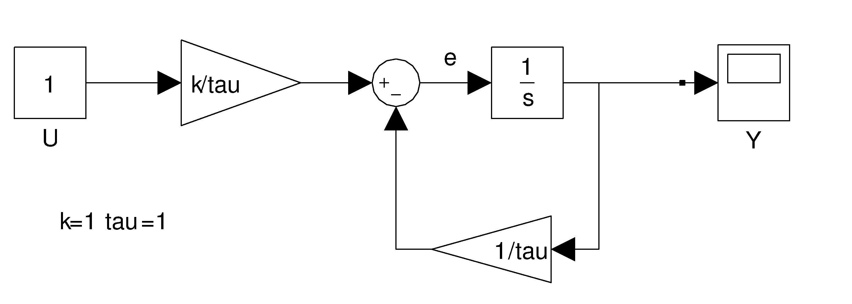
Figure 1: Academic example : First order transfert function

3.1.1 Symbolic derivative. Manual method using the transfer function

See subsection 2.12 for operational calculus formalism used here. Compute the equivalent transfer function. Write the equation between each block and resolve the causality:

$$\left(\begin{array}[]{lcl}e&=&-\frac{1}{\tau}Y+\frac{k}{\tau}U\\ Y&=&\frac{1}{s}e\end{array}\right)\quad\Longrightarrow\quad Y=\frac{kU}{1+\tau s}$$ (24)

Then, we have two possibilities. The first is to work in the Laplace domain.

$$\frac{dY}{d\tau}=\frac{-ks}{(1+\tau s)^{2}}U.$$ (25)

The second way is to transform the equation 24 in time differential equation like (equ. 26) :

$$y^{\prime}=\frac{-y+ku}{\tau}\Longrightarrow\frac{dy^{\prime}}{d\tau}=\frac{\left(-\frac{dy}{d\tau}+k\frac{du}{d\tau}\right)\tau+y-ku}{\tau^{2}}$$ (26)

with

$$\frac{du}{d\tau}=0.$$

For theses 2 ways (equ. 25) and (equ. 26), it is necessary to rewrite the equations in block diagram description and to make the time integration to get the expected result. We can also, when it is possible, compute a finite form solution (equ. 27) and derivate this one with respect to the independent parameters.

All these methods are not useful to keep the block diagram description but it is better that nothing when the model is simple.

$$y^{\prime}=\frac{-y+ku}{\tau}\quad\begin{array}[]{c}[b]\int\\ \longrightarrow\end{array}\quad y(t)=k\left(1-e^{-t/\tau}\right)u(t)\quad\begin{array}[]{c}[b]d/d\tau\\ \longrightarrow\end{array}\quad\frac{dy(t)}{d\tau}=\frac{kte^{-t/\tau}}{\tau^{2}}.$$ (27)

3.1.2 Finite difference with independent parameters

Often, this method is used with optimization algorithm and to compute the derivative with respect to parameter by finite difference. Nevertheless, it is very difficult to choose the epsilon value of the parameter. This method does not work well when we have noise on the input, strongly non linear equation or when we have discontinuities in the model ( step, hysteresis, etc) and it is very difficult to embed it in real time. The finite difference is not generally accurate and the optimization, even if we use a complex strategy of optimization, does not lead to the optimal solution due to the choice of epsilon. But all the engineers use it for small and big models.

3.1.3 Via computer algebra tools

We can use BlockImporter™ (which is a Maple add-on) that allows you to import a Simulink model into Maple and to convert it into a set of mathematical equations. Thus it is possible to analyze and derivate the equation in a reliable way. But the work is not finished, as it is necessary to translate the result back in the Simulink block diagram environment. It will be impossible to treat the blocks: discontinuities, logic evens and look-up table in the model, except if we decompose the model in piecewise continuous functions. Another hard issue will be closed form integration, which will not be possible in the general case, and may be very expensive in time and memory.

3.1.4 Automatic differentiation of code

We may try to convert the model in C or Fortran code and then call appropriate tools. For a short and didactic example, we use the on-line Automatic Differentiation engine TAPENADE. The routine model table 2 describes the equation(25): the dependent output variables are yprime, y and the independent parameter tau. We have chosen the option Fortran and differentiated in “TangenteMode”, we have obtained the differentiated program in table 3.

SUBROUTINE MODEL(yprime, y, u, tau, k) IMPLICIT NONE DOUBLE PRECISION yprime, y, u, tau, k yprime = (-y+k*u)/tau END

Figure 2: Source code

SUBROUTINE MODEL_D(yprime, yprimed, y, yd, u, tau, taud, k) IMPLICIT NONE DOUBLE PRECISION yprime, y, u, tau, k DOUBLE PRECISION yprimed, yd, taud yprimed = (-(yd*tau)-(y+k*u)*taud) /tau**2 yprime = (-y+k*u)/tau END

Figure 3: Differentiated program

Usually it is not possible to use the result of the automatic differentiation in real time. We face a lot of problems of compatibility between libraries, or related to the structures of languages, especially when we use triggers or enable blocks. Moreover we don’t have access at all the sources of the libraries, which is a major limitation to build embedded code.

3.1.5 Graphic derivative AGDM First derivative

An another way is to apply the rules described in the forthcoming paragraph 3.3 Rules for the automatic graphic differentiation Methodology (AGDM). With these rules, the model (Fig.1) can be written like in the following Figure 4. The rules are straightforward to implement.

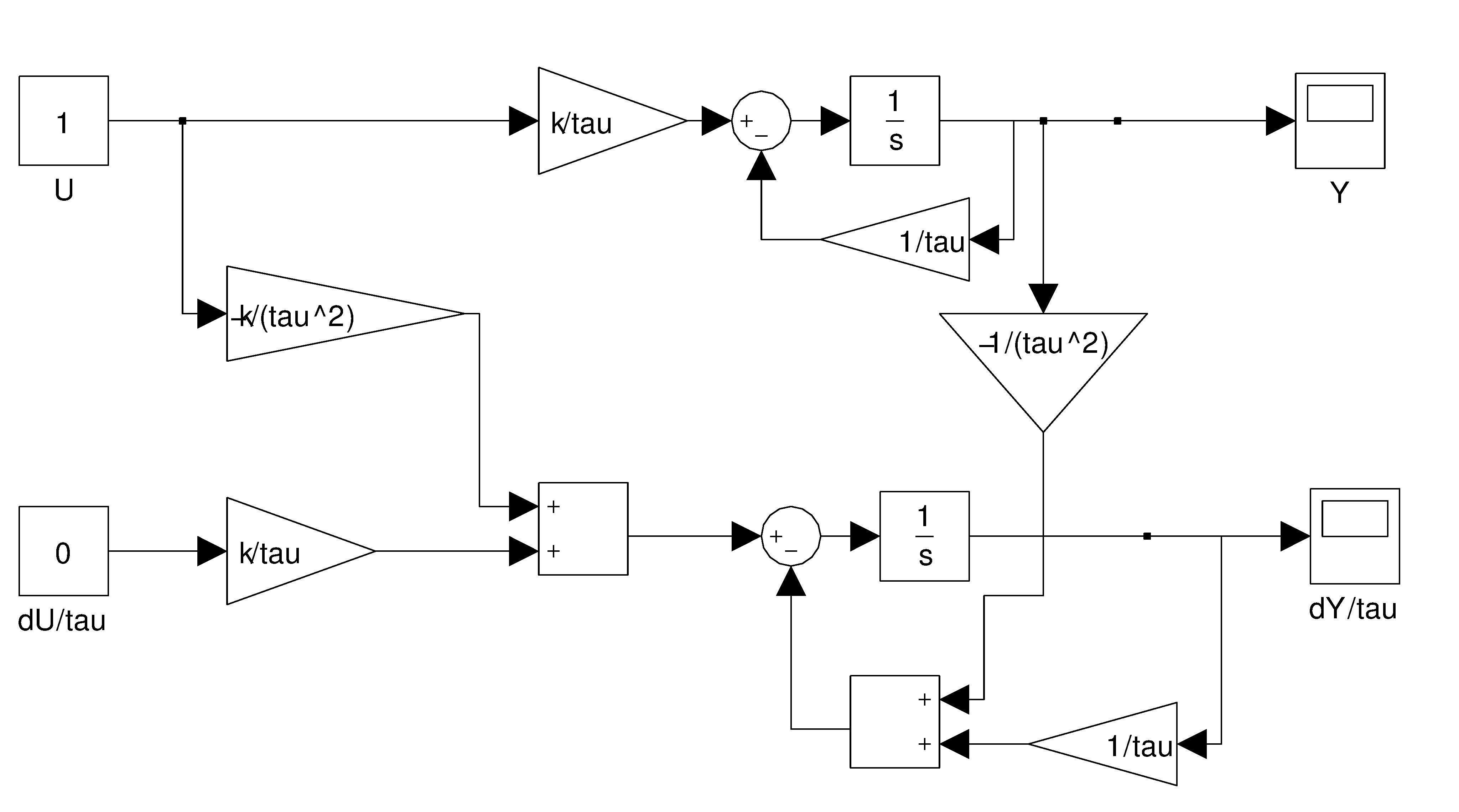
Figure 4: ADGM Order $1$

3.2 Computing the Hessian

Try to compute the hessian or the second derivative is very complicated for all the raisons explained before but also by the size of result too, except if the model is simple.

For example, if we start with the Equation 24, we obtain the Equation 28.

$$\frac{d^{2}Y}{d\tau^{2}}=\frac{2ks}{\left(1+\tau s\right)^{3}}U$$ (28)

But, the disadvantage which have been outlined is that we lost, in the condensed formula, the saturation of integrator. With ADGM it is possible to drive the integrator in the derivative flow by the saturation value in the original scheme (Fig. 1).

Via ADGM, it is necessary to apply the rules one more time on the model. The properties of the partial derivative are kept: $\frac{\partial^{2}Y}{\partial x\partial z}=\frac{\partial^{2}Y}{\partial z\partial x}$. However, to use an helpful automat like Diffedge will be appreciated and we obtain the Figure 5. If we compare by numerical simulation ( integration) the mathematical form of ADGM methology and the explicit derivative ( Second order) we obtain exactly the same result.

Figure 5: Hessien of original scheme ( Order 1)

3.3 Rules for Automatic Graphic Differentiation Methodology (AGDM)

The rules are based on the technical field of “Automatic Differentiation” to derive the conditional structures as well as the structural properties of block (math function, state,…) diagrams and by application of the formula for derivatives of composite functions. Seven simple rules of differentiation, including two rules on the links ( J) and five on the blocks (M) allow to automatize the process of differentiation which can be manual or by computer using a computer algebra system like Maple . All these rules can differentiate easily a model described as pattern blocks (SISO, MIMO, continuous / sampled, finite state) systems Applying all these rules are possible because we use the structural property (flow causality, block independent,…) of bloc diagram representation. Each block is independent, in other words it does not depend on other block around it and is self-standing. This guarantees that all blocks in the block diagram can be differentiated independently of each other. Furthermore, we use the causality property of the block diagram. The derivative flow propagates like the causality flow.

Finally, with these rules we obtain the block diagram differentiated with respect to the parameter k. The user benefice is very important because the derivative model is also a block diagram and like that, we still have access at all the functionality of Matlab/Simulink (optimization, real time etc.). This method is definitively the best and the most powerful way to get the symbolic derivative instead of translating the model in equations and then derivate them. For understanding these rules, one may look to their application on the figures (Fig.1),(Fig.4) and (Fig.5).

3.3.1 Link rules: J1 and J2

J1

Whatever the block through by the differentiated flow, all its outputs will be affected by it. This rule can be applied for scalar links, vector and matrix. For example multiplexor, demux, subsystem, etc (see 6)

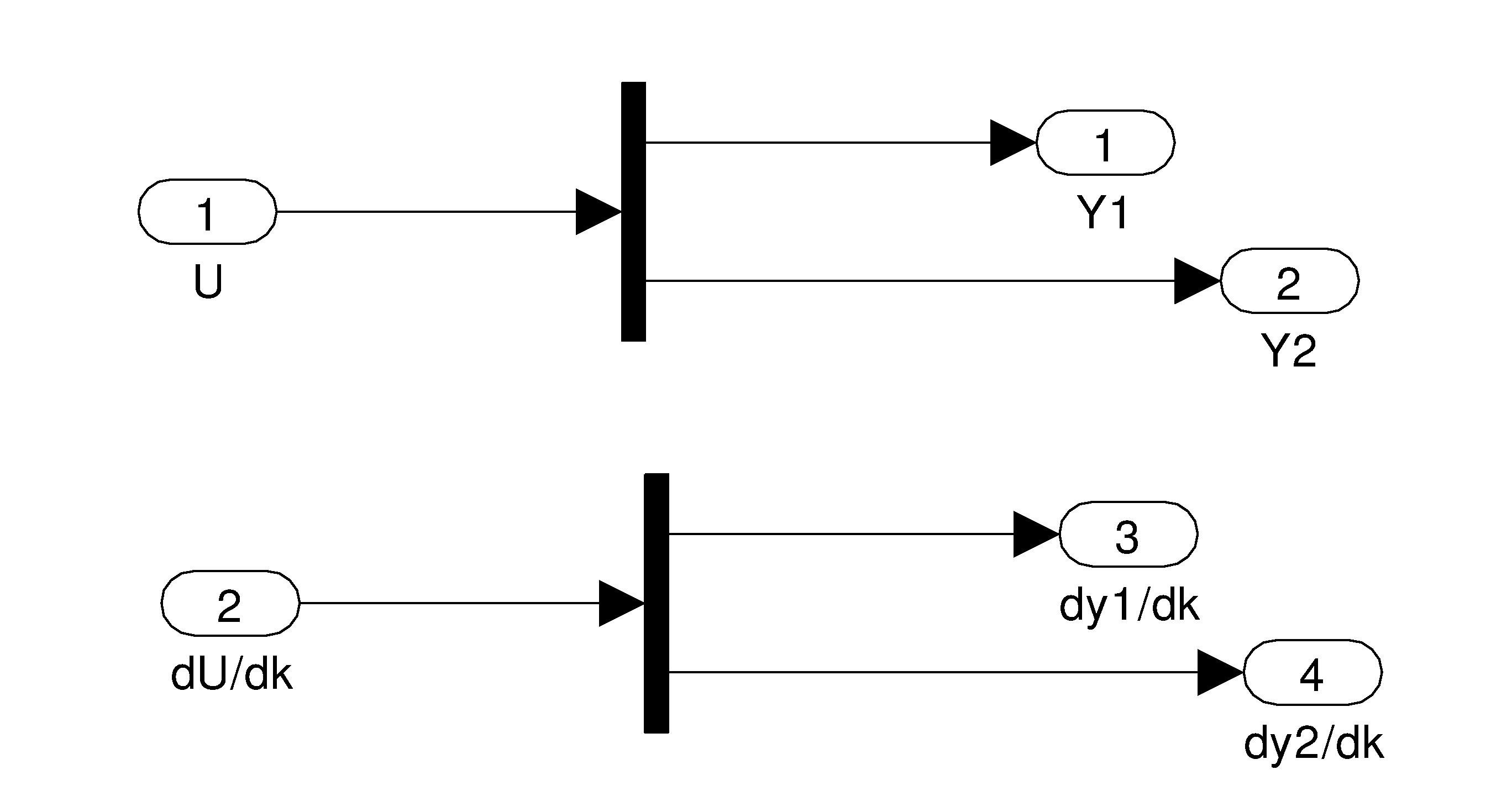
Figure 6: J1 rule applied to Mux block

J2

All blocks unaffected by the derivative flow and not depending on derivative parameter can be considered as a constant source equal to zero like constant block, sourcefrom workspace , etc In other words, when the inputs do not carry the flow derivative with respect to derivative parameter, the block does not appear in the derivative block diagram. This rule is useful for simplifying the derivative model. (see 7)

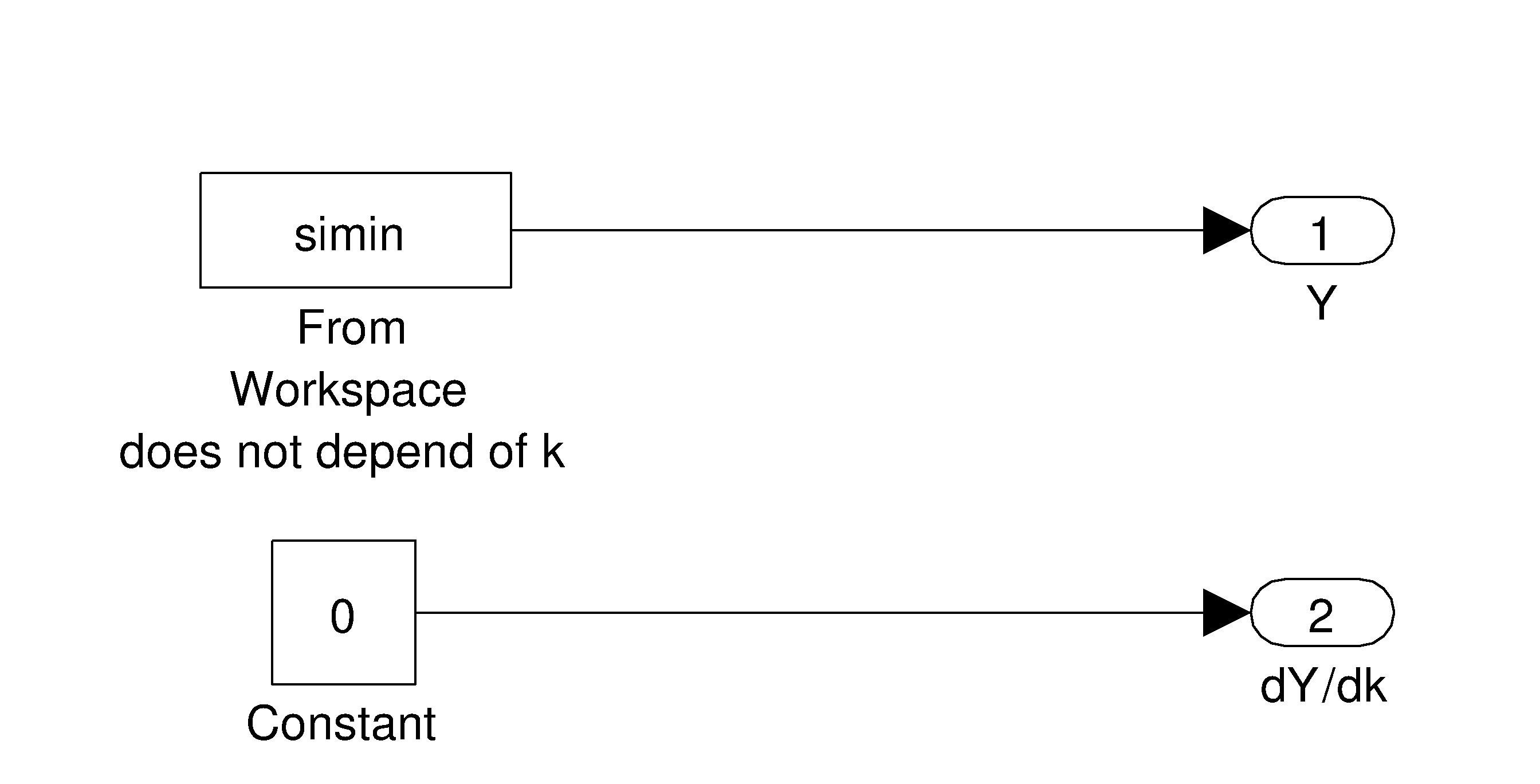
Figure 7: J2 rule derivative block independent of the parameter

3.3.2 Block rules M1, M2, M3, M4, M5

M1

All the inputs/outputs of each of block and the sub-block of the original scheme should be accessible at every step time of the simulation. Because it is necessary to have the mathematical function of each block to obtain the derivative scheme. Moreover, each subsystem is increased of the derivative flow. For instance, the subsystem with 2 inputs and 1 output differentiated with respect of 2 parameters k2 and k2 gives the following:

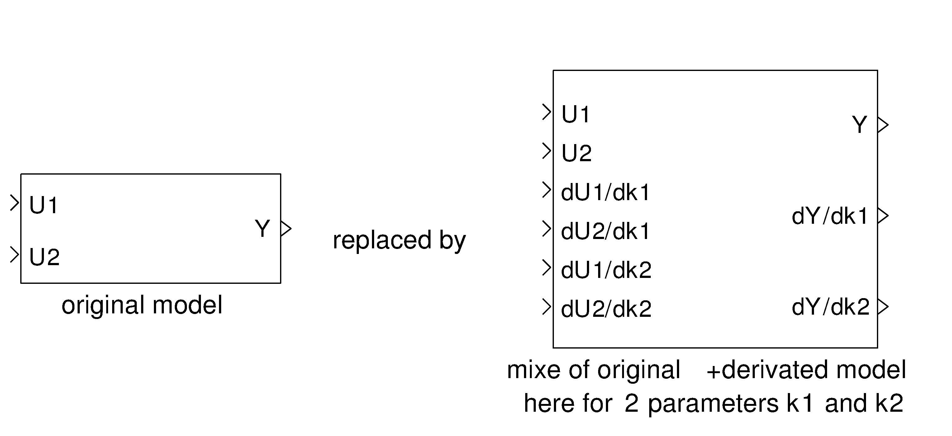
Figure 8: Derivative subsystem

M2

For all linear blocks H(k) in U through by differentiated flow we can built the following scheme that contains the original block diagram increased of derivative with respect to a parameter k.(Fig. 9)

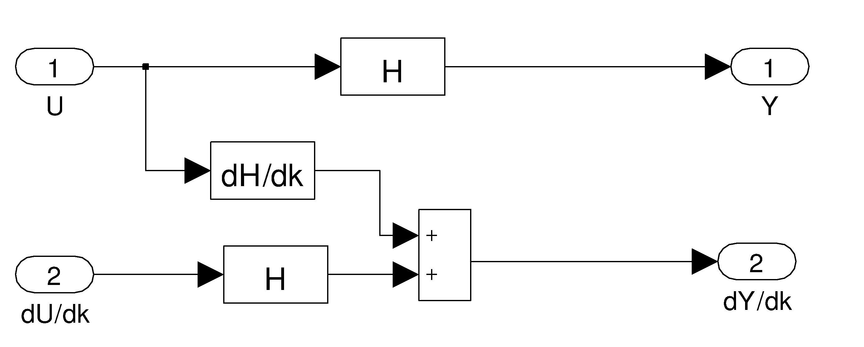
Figure 9: M2 rule for alinear block depending on of the parameter $k$

If the block does not depend of derivative parameter, we obtain the diagram below (figure 10).

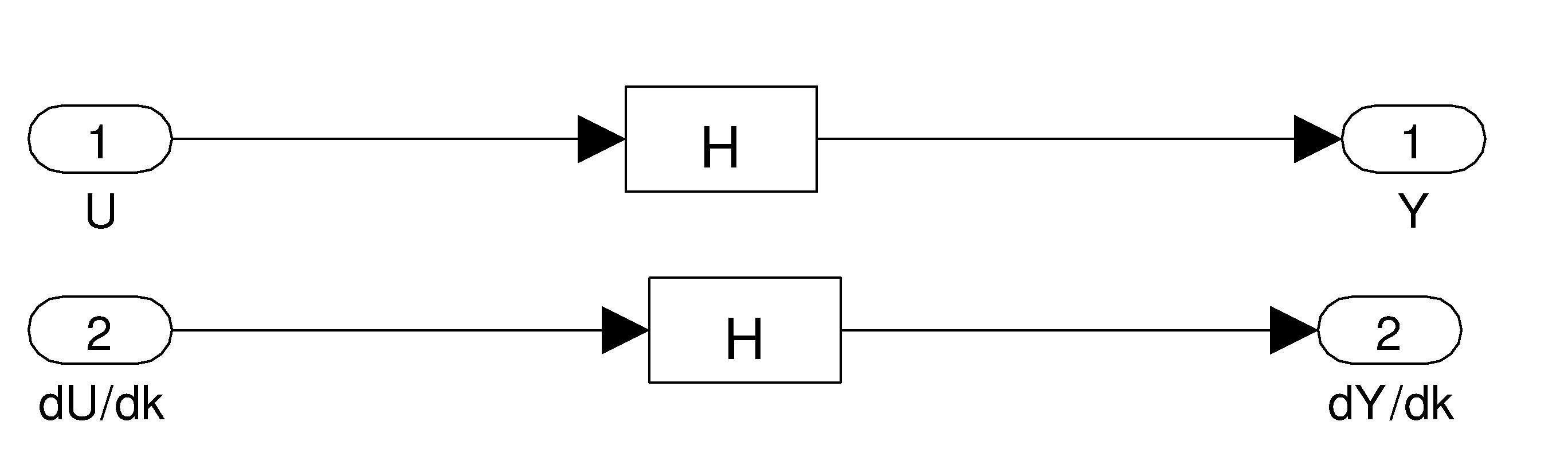
Figure 10: M2 rule for linear block without parameter

In fact, when the blocks are linear and do not depend on the differentiation parameter, we just need to duplicate the model into the derivative flow. We will increase the original model as many times as there are parameters with respect to which differentiation is performed.

M3

For a nonlinear block we write

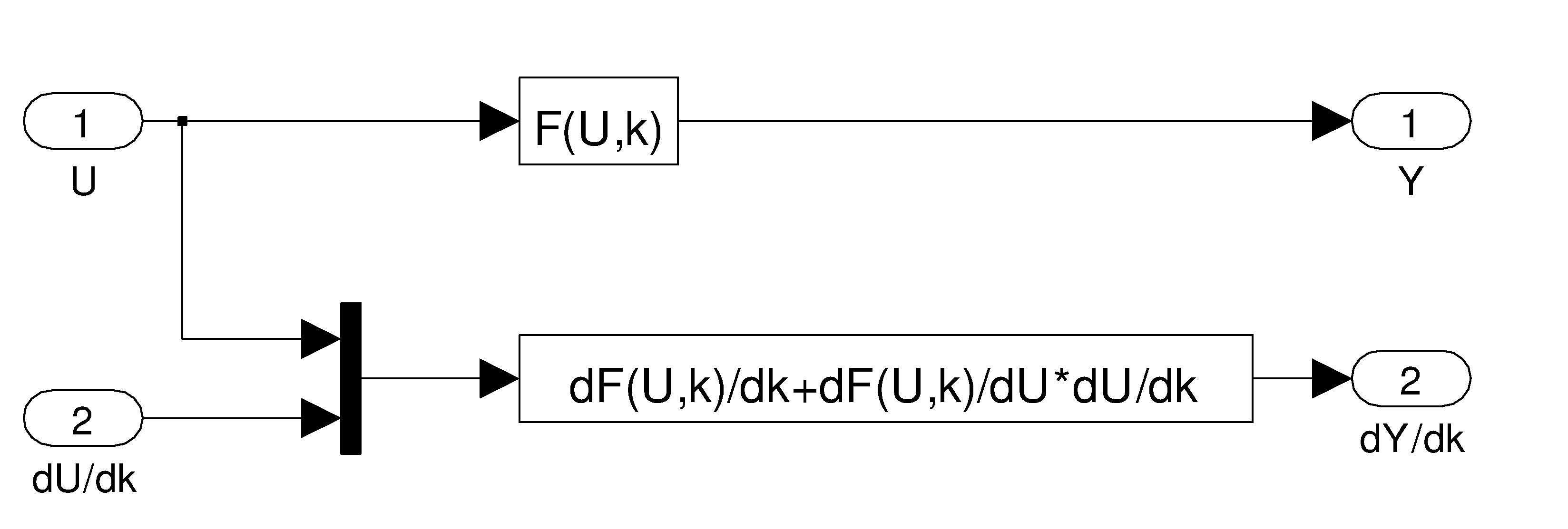
Figure 11: M3 for non linear block in Laplace or Z

In this case, it may be necessary to use a computer algebra system to compute the derivatives, accordiing to the mathematical definition of the block.

M4

For a conditional block (Switch, hysteresis, max, min, trigger subsystem, logic( and, or,etc) , stateflow…, saturated integrator …) which is defined by a piecewise or event function, we duplicate the block and we keep the same logical tests as in the original block but the outputs contain the derivative flow. According to automatic differentiation, the threshold of logical blocks has not to be differentiated.(figure 12)

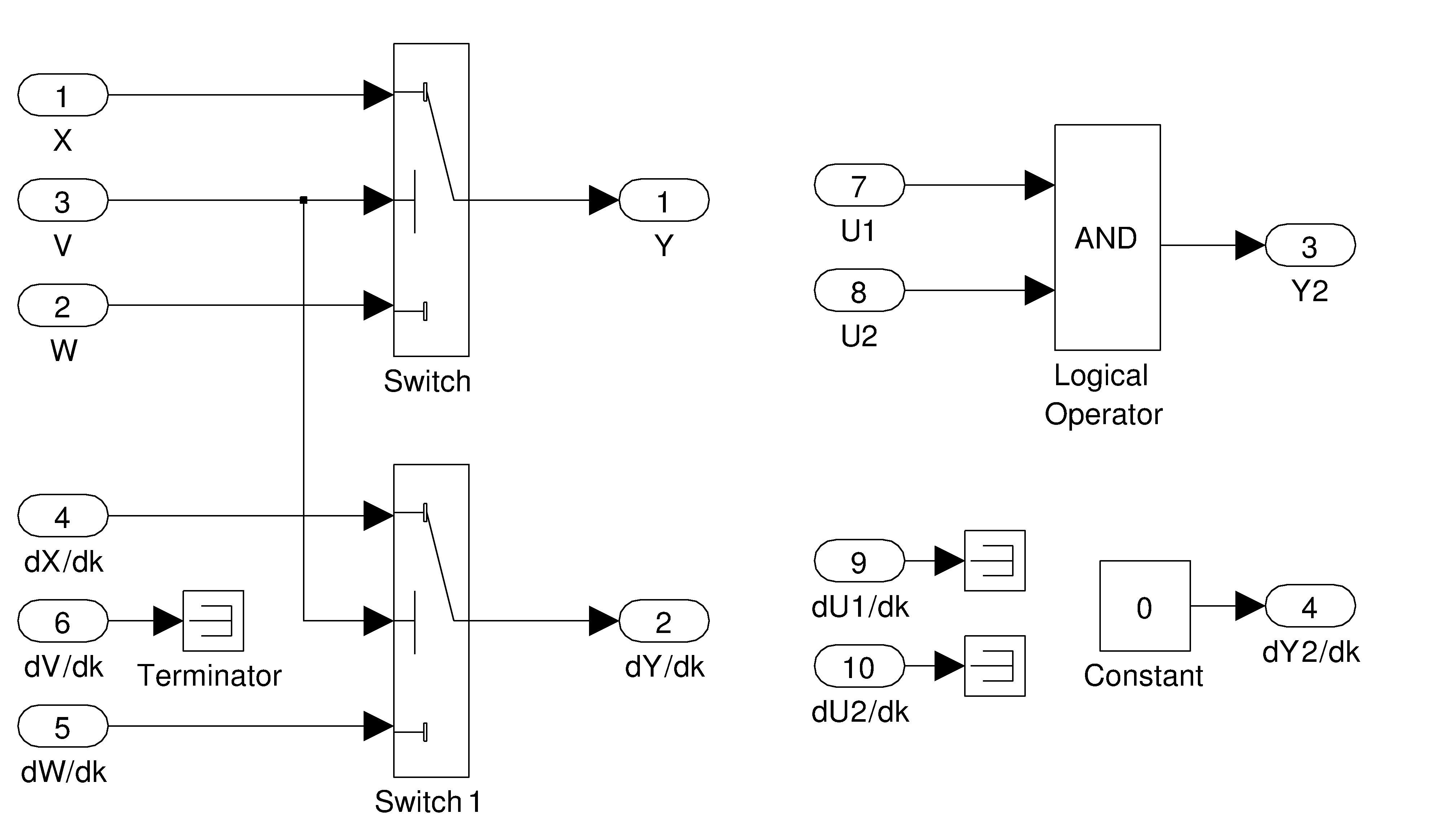
Figure 12: M4 rule on switch and AND block

M5

In the case of “black box” block, such as a lookup table 1D, $n$D or S-function, the mathematical equations are not accessible and nothing can be done in the case of lookup tables. So we need to retreat to finite difference. E.g. in the case of a function $y(x,k)=f(x,k,u(x,k))$, we obtain an evaluation of the derivative $\frac{df}{du}=\frac{\partial f}{\partial k}+\frac{\partial f}{\partial u}\frac{\partial u}{\partial k}$:

$$\frac{dy(k,u(k))}{dk} =\frac{f(x,k+\epsilon_{k},u(x,k+\epsilon_{k})-f(x,k,u(x,k))}{\epsilon_{k}}$$

$$+\frac{f(x,k,u(x,k)+\eta_{u(k)})-f(x,k,u(x,k))}{\eta_{u(k)}}\frac{\partial u(k)}{\partial k}.$$ (29)

The best choice of the increment $\eta_{u(k)}$ of the input $u(k)$ is the step between 2 values of $u(k)$ input values of a lookup table. In general, the choice of the increment $\epsilon(k)$ may require many tests befor finding a proper value and it is better to adapt the choice for each lookup table or black box block rather than using a single value $\epsilon$ for the whole model.

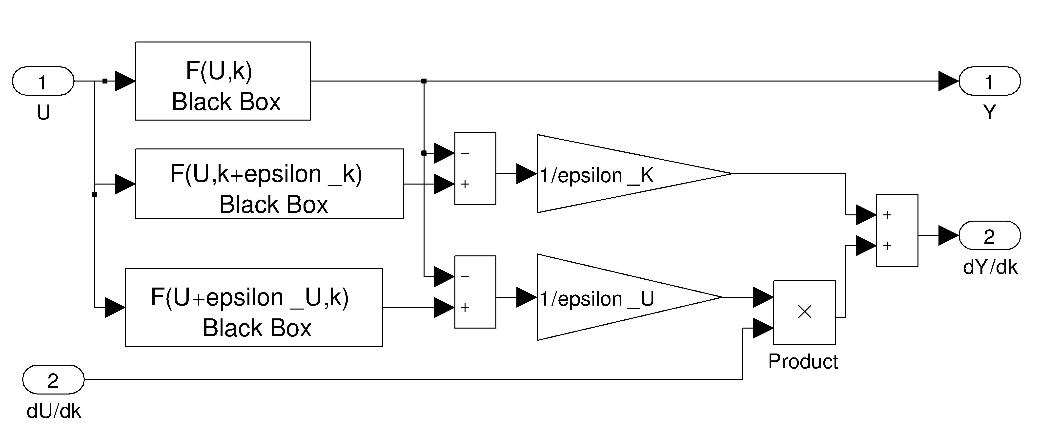
Figure 13: M5 rule for Black box

All the rules introduced above are sufficient to compute the derivative model of all Simulink models and for specifying an automata computing the derivative like Diffedge.

3.3.3 Other mathematical representation

This notion of graphic derivative may be generalized to all mathematical objects like continuous transfer and state space but also to discrete transfer function and state space. It is thus possible to build the gradient of hybrid models. For instance, in the case of continuous state space JM’s rules give the original state-space increased of the derivative flow

Continuous case

$$\left\{\begin{array}[]{lcl}\dot{X}&=&AX+BU\\ Y&=&CX+DU\end{array}\right.\Longrightarrow\left\{\begin{array}[]{lcl}\left(\begin{array}[]{c}\dot{X}\\ \frac{d\dot{X}}{dk}\end{array}\right)&=&\left[\begin{array}[]{cc}A&0\\ \frac{dA}{dk}&A\end{array}\right]\left(\begin{array}[]{c}X\\ \frac{dX}{dk}\end{array}\right)+\left[\begin{array}[]{cc}B&0\\ \frac{dB}{dk}&B\end{array}\right]\left(\begin{array}[]{c}U\\ \frac{dU}{dk}\end{array}\right)\\ \left(\begin{array}[]{c}Y\\ \frac{dY}{dk}\end{array}\right)&=&\left[\begin{array}[]{cc}C&0\\ \frac{dC}{dk}&C\end{array}\right]\left(\begin{array}[]{c}X\\ \frac{dX}{dk}\end{array}\right)+\left[\begin{array}[]{cc}D&0\\ \frac{dD}{dk}&D\end{array}\right]\left(\begin{array}[]{c}U\\ \frac{dU}{dk}\end{array}\right)\end{array}\right.$$ (30)

Discrete case

For the Discrete case, we have the same structure with the following notation: $\dot{X}=X_{n+1}$ and $X=X_{n}$ and idem for $U$ and $Y$.

In Simulink The Discrete Transfer function block implements the z-transform transfer function described by $z^{n}$ or $z^{-n}$ power with the following equations in z:

$$H(z)=\frac{b_{0}+b_{1}z+\cdots+b_{m}z^{m}}{a_{0}+a_{1}z+\cdots+a_{m}z^{m}}\quad\hbox{with}\quad m\leq n.$$ (31)

3.4 Other examples

Simulink blocks have often dissimulate complex structures. It may then be necessary to rewrite theses blocks using elementary blocks to be able to apply the rules and compute the derivative of blocks such as Min, Max, etc.

Discontinuous block:

For example, we propose to differentiate the Saturation Dynamic block (the bounds range of the input signal to upper and lower saturation values). The input signal outside of these limits saturates to one of the bounds low or up port. We suppose, the bounds do not depend of the parameter.

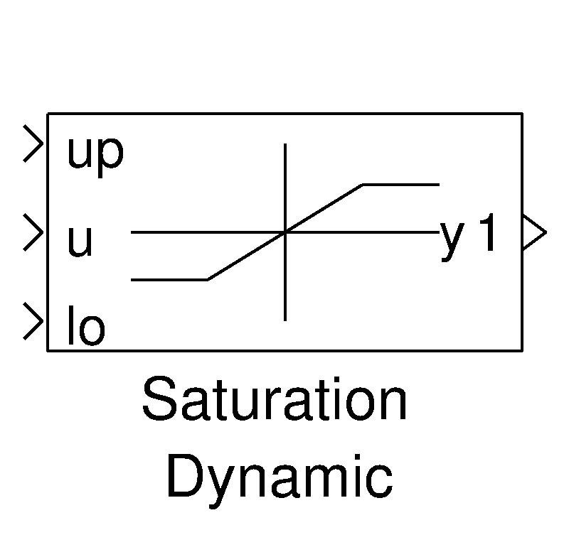
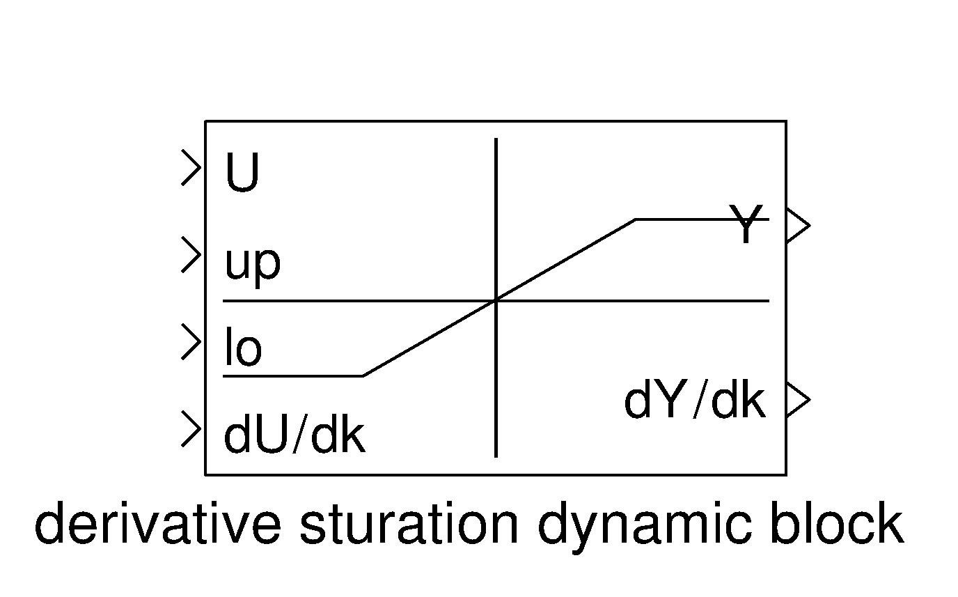
Figure 14: Saturation Dynamic block (left) and its derivative (right)

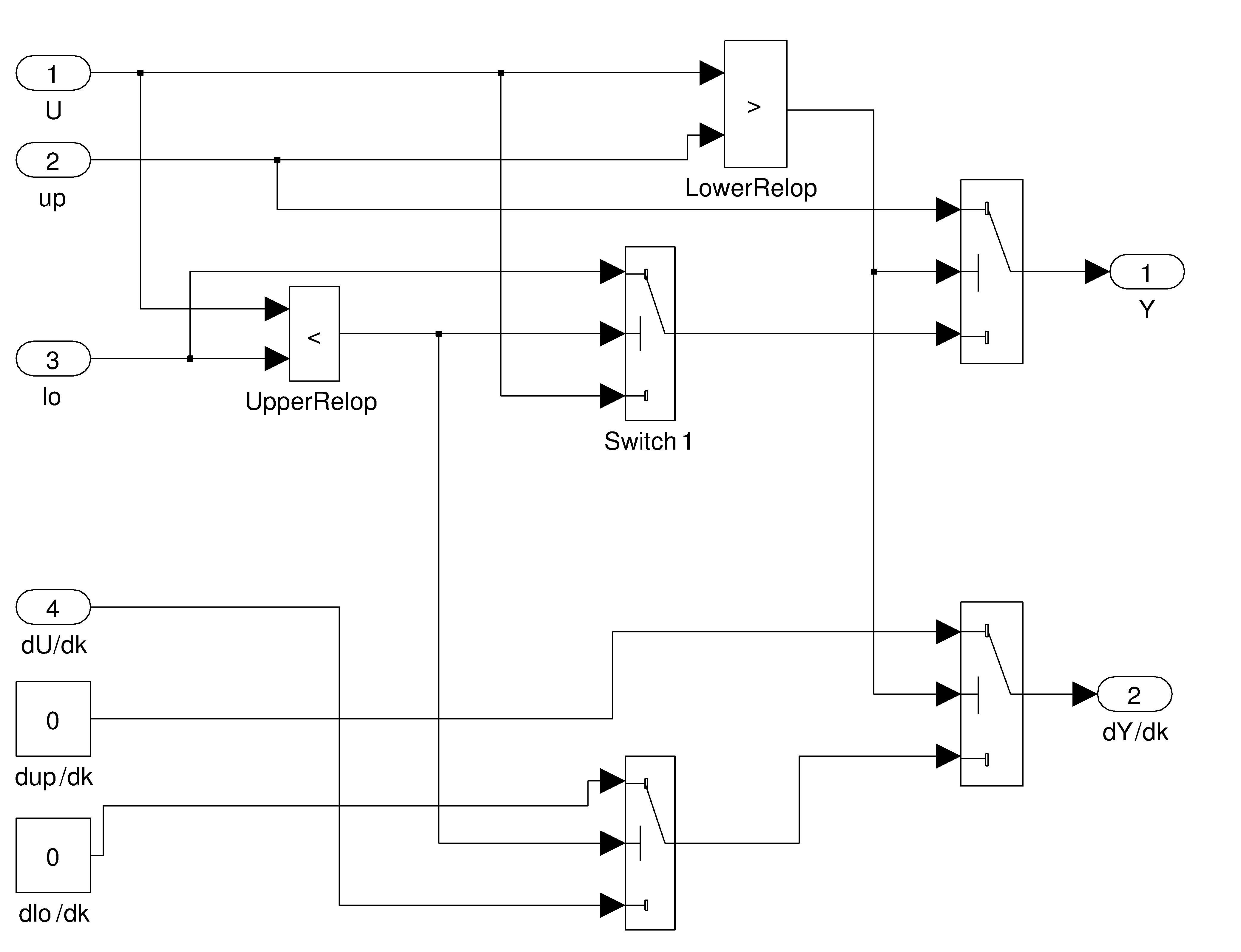
Figure 15: Inside the Derivative of Saturation dynamic block

Discrete block.

We want to study the sensibility of the parameter k inside of discrete integrator, it is necessary to compute the derivative (Fig. 16)

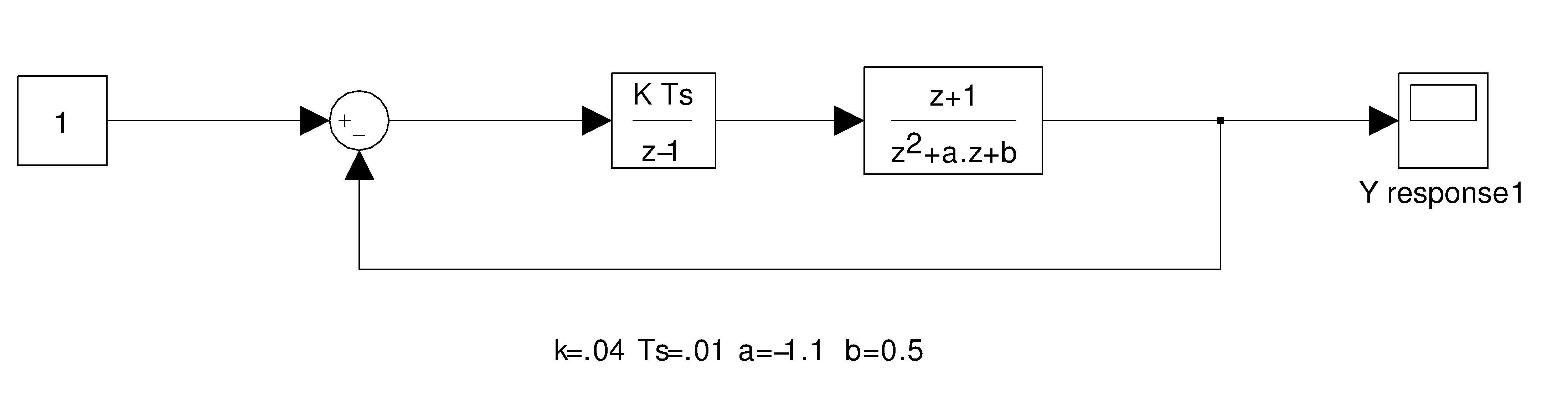
Figure 16: Discrete representation

Application of rules gives the Fig. 17 For computing the derivative of the (Fig. 16), we duplicate the original model. We just put the source at zero and link the derivative of the integrator with respect to K just after the add block then finally we put a additional block in the derivative flow.

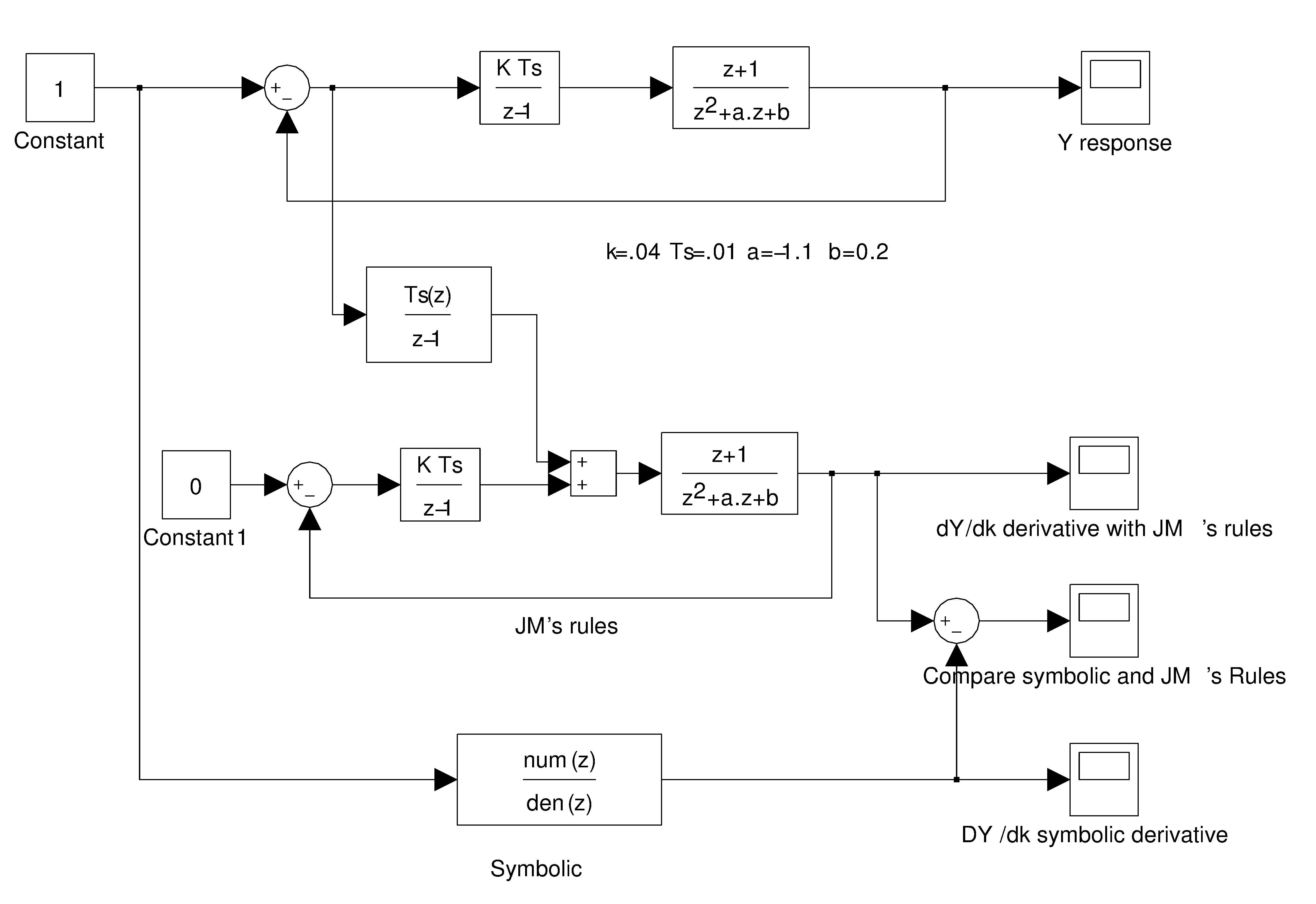
Figure 17: Discrete derivative representation

And at last, we compare the ADGM with the evaluated derivative. This last one step is very complicated to obtain. We have to evaluate the close loop, to compute the derivative with respect to k and to convert it into a rational fraction in canonic form that will be entered in the dialogue discrete box of Simulink. The next formula expresses the formal derivative and is implemented in the “Symbolic” block of fig. 17.

$$\frac{dY(z)}{dk}=\frac{Ts\left(z^{4}+az^{3}+\left(b-1)\right)z^{2}-az+KTs-b\right)-KTs^{2}}{\left(z^{3}+\left(a-1\right)z^{2}+\left(KTs-a+b\right)z+KTs-b\right)^{2}}.$$ (32)

The result obtained with ADGM is exactly equal to what we get frrom the integration of equation 32, with less effort.

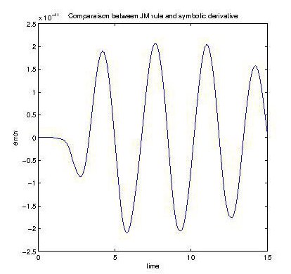
Figure 18: Error between the true and ADGM derivative

The best way for computing the derivative is to use JM’s rules It is very simple, efficient, fast and useful. This method is also a good way for optimizing Finite Response Input (FIR) filters with saturation.

3.5 An example of optimization

We conclude this section with a classical example. We consider a second order system and try to minimize the energetic cost of the transitory behaviour during a step action. Our second order system is the following (Fig. 20).

$$x^{\prime\prime} = -2\zeta\omega x^{\prime}-\omega^{2}x+\omega^{2}u(t)$$ (33)

$$y = x$$ (34)

The initial conditions are $x(0)=0$ and $x^{\prime}(0)=0$ and $u(t)$ the Heaviside function $u(t)=0$ if $t<0$ and $u(t)=1$ if $t\geq 0$.

We want to minimize

$$J(\zeta)=\int_{0}^{\infty}(\omega^{2}e(t)^{2}+q^{2}e^{\prime}(t)^{2}){\rm d}t,$$

with $e(t)=x(t)-u(t)$.

In this simple case, a simple Maple computation will provides the optimal value of $\zeta$ with $q=1$ and $\omega=1$ is $\zeta=\frac{sqrt(2)}{2}=0.7071067811865475$ with 16 Digits. We will use it to illustrate how Diffedge can be used for optimization. For this, we need to compute $(\partial J/\partial\zeta)(\zeta)$, in order to use the Levnberg–Marquardt algorithm, implemented in Matlab fsolve function. The time of simulation is 10 sec.

Our goal is to compare AD and finite difference in real world condition(by example embedded optimization on micro computer), many practical examples encountered in engeneering practice being close to this archetypic problem wherever the sample time of the observation is large.

Remark.

One must be carefull to the sensibility of the computation of the integral $J$ with respect to the time observation frequency: not enought points will give a poor precision in optimization, but too many points can cumulate inacuracies and finite difference method will be very sensitive to such computational noise. The time observation is given by the block rate transition with the variable $Tsample$. Here after (fig. 19, we show two responses with differente values of $Tsample$. One may notice that there are too few points in the sample here to use finite difference but that AGDM still works.

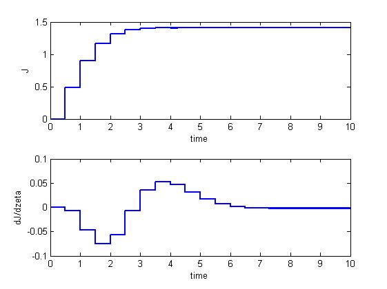
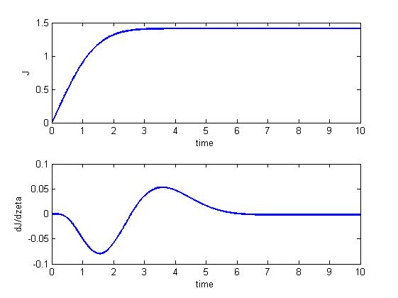
Figure 19: Tsample=$0.5$ seconds (left) and Tsample$=0.005$ seconds (right)

Differentiation.

The corresponding block diagram of these equations can be written in the following way (Fig. 20). Following classical engeneering practice, one may use Heaviside operational calculus and represent our equations by a unit feedback of the open loop system described by the transfer function

$$\frac{\omega^{2}}{s(2\omega\zeta+s)}.$$

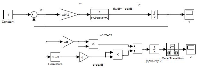
Figure 20: Second order with cost function J

In this model, the cost is simulated together with the initial model. One may notice that, for the sake of genericity, the derivative $e^{\prime}(t)$ is computed using the block derivative, that uses finite difference, that may penalize accuracy. But, if $u$ were not constant for $t\geq 0$, we would have no other choice, as $e^{\prime}=x^{\prime}+u^{\prime}$, except if $u$ is itself defined in such a way that AD can be used for it. The differentiated model, described by the following (fig. 20). is obtained by duplicating the initial model (fig. 21). and applying the rules:

— J2 on the constant;

— M2 on the linear block depending on $\zeta$;

— M3 on the nonlinear blocks like multiplication.

Modifications with respects to the initial model appear in red.

The optimization program to be used here is the following. The output ${\rm d}J/{\rm d}\zeta$ of our differentiated block diagram is embedded in the myfcost function.

function [J,Jacobian] = myfcost(zeta)
zeta=min(zeta,3);zeta=max(.001,zeta);
assignin(’base’,’zeta’,zeta)
sim(’mymod’);
out=eval(’base’,’out’);   % get J in the  workspace
dout=eval(’base’,’dout’); % get dJ/dzeta  workspace
J=out;                    % Objective function
if nargout > 1            % Two outputs argument
Jacobian = dout;          % Jacobian of the function (ADGM)
end

To launch optimization, where $\zeta$ is initialized to the value $0.1$, one uses the following syntax with option on for ADGM/Symbolic or off for finite differences, when computing the Jacobian.

[zeta_opt,fval,exitflag,output]=fsolve(@myfcost,[.1],optimset(’Jacobian’,’on’))

One may compare the obtained value to the theoretical solution of $\zeta$.

Rate transition	Matlab jacobien	ADGM jacabien
(time observation)	(finite difference)	(symbolic)
		Theorical $\zeta=0.7071067811865475$
0.5	Zeta_opt= 0.1	Zeta_opt=.70698585
	1 iterations	9 iterations
	funcCount: 22	funcCount: 23
0.1	Zeta_opt= 0.10154269	Zeta_opt=0.71180603
	8 iterations	8 iterations
	funcCount: 40	funcCount: 25
0.07	Zeta_opt= 0.10089164	Zeta_opt= 0.70857782
	4 iterations	7 iterations
	funcCount: 29	funcCount: 24
0.04	Zeta_opt= 0.10062591	Zeta_opt= 0.71130072
	5 iterations	9 iterations
	funcCount: 32	funcCount: 22
0.01	Zeta_opt= 0.70625955	Zeta_opt= 0.70671083
	9 iterations	9 iterations
	funcCount: 29	funcCount: 19
0.005	Zeta_opt= 0.70630892	Zeta_opt= 0.70628714
	9 iterations	9 iterations
	funcCount: 29	funcCount: 29

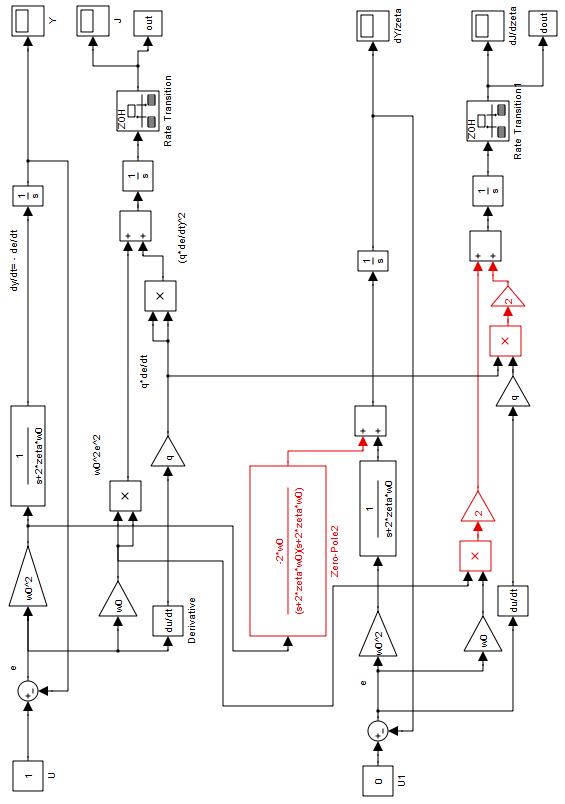
Figure 21: Second order derivative with respect to $\zeta$

The number of observation points does not improve the result. In our case the solver is ode45 and the relative tolerance is $rtol=10^{-7}$. This means that the computed state ($J$) is accurate to within 0.00001% It is not possibe to get better precision than around $\approx 10^{-4}$ even using symbolic jacobian. But we notice that the optimization with a symbolic jacobian is more reliable.

4 Testing the precision

It seems safe to complete this presentation with a few hint to test the robustness of the obtained results. Most of the time, it is of course impossible to compare results using an extra tool with certified reliability. And if the result of the other tool is not somehow “certified”, a third one would be required, in case of discrepancies, assuming that if two methods agree they are likely to be right.

However, any numerical tool may be tested on a set of known systems that already may give an idea of its possibilities and help to test it during its development.

4.1 Symbolic computation

The possibilities are obvious enough to dispense us of lengthy developments, but as most differential systems do not have closed form solution, let us stress that the safest way would be a start by the solution and reconstruct the system. Chained systems provide an easy way to build systems of increasing size and complexity when keeping symbolic resolution fast.

4.2 Flat systems

Flat system, already menstionned above (see 2.3.1), are a special class of differential systems with a closed form solution, including well known chained examples of arbitrary size, like the car with $n$-trailer [23] or many discretization of flat inifinite dimensional systems [59]. Such examples where used with success during the tests of the rocket engine simulator Carins [61], allowing to detect a bug in Maxima.

4.3 Interval arithmetics

As interval arithmetic can garanty that the result belongs to the result interval, it may also be used to test any numerical tool. The computer algebra system Mathemagix includes a package numerix for intervals and also balls with certified arithmetics [44, 42].

Conclusion

We have shown that, if the advantages of AD are obvious, one needs to be carefull in many cases of great pratical interest, where its naive use may lead to inaccuracies. A clever use requires a high level knowledge of what subroutines are made for, that is not just their syntax but also semantics. E.g. we have shown that differentiating a loop heavily depends on the fact that the loop is assumed to converge to a fixed point, or not. In the worse case, automatic procedures will be unable to recover the semantic hidden behind the syntax, which may lead to unavoidable inaccuracies. The best solution would be to generate numeric code from symbolic formulae, allowing more flexibility if new expressions, such as a derivatives, are required. But the available tools are still limited.

Simulink block diagrams offer a perfect illustration of high level object that may—and must—be differentiated as high level object, leading to better accuracy and keeping the benefit of their wide range of possibilities, including translation in Fortran or C to incorporate of real time optimization routines in embeded code. To some extend, Simulink block diagram description offers a better and more flexible framework to compute gradients with AGDM methodology that what is offered, not only by low level coputer languages like C or Fortran, but also by computer algebra systems like Maple, with the restriction of discontinuities that cannot be handled properly and require the use of continuous approximations using $\arctan$.

Being able to produce numerical programs that could be efficient and flexible, i.e. that could easily produce extra outputs such as derivatives, remains a challenge for software engineering. Producing numerical code from computer algebra specification is a part of the answer, but we need to adapt our tools to produce not only matematical formulas, but programs that must be fast and well conditionned. For the present time, we still have to cope with the necessity of pluging AD features on softwares that have not been thought in advance to facilitate the task or even make it possible and safe.

References

- [1] Arbogast, (Louis François Antoine), Du calcul des dérivations, Levrault frères, Strasbourg, an VIII (1800).
- [2] Bastogne (Thierry), Thomassin (Magalie), Masse (John), “Selection and identifcation of physical parameters from passive observation. Application to a winding process” Control Engineering, Practice, Elsevier, 2007, 15 (9), pp.1051-1061.
- [3] Baur (Walter) and Strassen (Volker), “The complexity of partial derivatives”, Theoretical Computer Science, 22, 317-330, North-Holland, 1983.
- [4] Beck (Thomas) and Fischer (Herbert), “The if-problem in automatic differentiation”, Journal of Computational and Applied Mathematics, 50, 119–131, 1994.
- [5] Beck (Thomas) “Automatic differentiation of iterative processes”, Journal of Computational and Applied Mathematics 50, 109–118, 1994.
- [6] Bell (Bradley M.) and Burke James V., “Algorithmic differentiation of implicit functions and optimal values”, chapter in Advances in Automatic Differentiation, Lecture Notes in Computational Science and Engineering vol. 64, 67–77, Springer 2008.
- [7] Bliss (Gilbert Ames), “The solutions of differential equations of the first order as functions of their initial values”, Annals of Mathematics, Second Series, Vol. 6, No. 2, 49–68, 1905.
- [8] Bliss (Gilbert Ames), “Solutions of differential equations as functions of the constants of integration”, Bull. Amer. Math. Soc. vol.25 , 15–26, 1918.
- [9] Boulier (François), Lemaire (François) and Moreno Maza (Marc), “PARDI !”, International Symposium on Symbolic and algebraic computation 2001, ACM Press, 38–47, 2001.
- [10] Boulier (François), Lazard (Daniel), Ollivier (François) and Petitot (Michel), “Computing representations for radicals of finitely generated differential ideals”, Special issue Jacobi’s Legacy of AAECC, J. Calmet and F. Ollivier eds., 20, (1), 73–121, 2009.
- [11] Boulier (François), Bibliothèques Lilloises d’Algèbre Différentielle, free sotware developped in C. http://www.lifl.fr/ boulier/pmwiki/pmwiki.php?n=Main.BLAD
- [12] Bostan (Alin), Chyzak (Frédéric), Salvy (Bruno), Lecerf (Grégoire) and Schost (Éric), “Differential Equations for Algebraic Functions”, Proceedings of ISSAC’07, 25–32, ACM, New-York, 2007.
- [13] Alin (Bostan), Chyzak (Frédéric), Ollivier (François), Schost (Éric), Salvy (Bruno) and Sedoglavic (Alexandre), “Fast computation of power series solutions of systems of differential equations”, Proceedings of 18th ACM-SIAM Symposium on Discrete Algorithms, 1012–1021, 2007.
- [14] Bronstein (Manuel), ElementaryFunction, Axiom (Scratchpad II) package, 1987. http://axiom-wiki.newsynthesis.org/SandBoxElemntry
- [15] Christianson (Bruce), “Automatic Hessians by reverse accumulation”, IMA J. Numer. Anal., 12 (2), 135-150, 1992.
- [16] Dickinson (Robert P.) and Gelinas (Robert J.), “Sensitivity analysis of ordinary differential equation systems – A direct method”, Journal of Computational Physics 21, 123–143, (1976).
- [17] Dridi (Mehdi), Dérivation numérique : synthèse, application et intégration, PhD thesis, École centrale de Lyon, 2010.
- [18] Dubois (François), Le Meur (Hervé) and Reiss (Claude), “Mathematical modeling of antigenicity for HIV dynamics”, Maths In Action, 3, (1), (2010), 1–35.
- [19] Elsheikh (Atiyah) and Wiechert (Wolfgang), “Accuracy of Parameter Sensitivities of DAE Systems using Finite Difference Methods”, IFAC Proceedings Volumes, Volume 45, Issue 2, 136–142, 2012.
- [20] Elsheikh (Atiyah), “An equation-based algorithmic differentiation technique for differential algebraic equations”, Journal of Computational and Applied Mathematics, 281, 135–151, 2015.
- [21] Estévez Schwarz (Diana) and Lamour ( René), “Diagnosis of singular points of properly stated DAEsusing automatic differentiation”, Numer. Algor. 70, 777–805, 2015.
- [22] Fliess (Michel), Join (Cédric) and Sira-Ramírez (Hebertt), “Non-linear estimation is easy”, Int. J. Modelling Identification and Control, Inderscience Enterprises Ltd., 2008, Special Issue on Non-Linear Observers, 4 (1), 12-27.
- [23] Fliess (Michel), Lévine (Jean), Martin (Philippe) and Rouchon (Pierre), “Flatness and motion planning: the car with n trailers”, European Control Conference, 1518–1522, 1993.
- [24] Fliess (Michel), Lévine (Jean), Martin (Philippe) and Rouchon (Pierre), “Flatness and defect of nonlinear systems: introductory theory and applications”, Internat. J. Control, 61, p. 1327–1887, 1995.
- [25] Fliess (Michel), Lévine (Jean), Martin (Philippe) and Rouchon (Pierre), “Deux applications de la géométrie locale des diffiétés”, Annales de l’IHP, section A, 66, (3), 275–292, 1997.
- [26] Fliess (Michel), Lévine (Jean), Martin (Philippe) and Rouchon (Pierre), “A Lie-Bäcklund approach to equivalence and flatness of nonlinear systems”, IEEE AC. 44:922–937, 1999.
- [27] Gebremedhin (Assefaw Hadish), Manne (Fredrik) and Pothen (Alex), “What color is your Jacobian? Graph coloring for computing derivatives”, SIAM Rev, 47, 629–705, 2005.
- [28] Gilbert (Jean-Charles), Le Vey (Georges) and Masse (John), La différentiation automatique de fonctions représentées par des programmes, Tech. rep. 1557, INRIA, 1991.
- [29] Glocker (Ch.), “Concepts for modeling impacts without friction”, Acta Mechanica 168, 1–19, 2004.
- [30] Gower (R. M.) and Mello (M. P.), “A new framework for the computation of Hessians”, Optimization Methods and Software, 27, (2), 2012.
- [31] Gower (R. M.) and Gower (A.L.)“Higher-order reverse automatic differentiation with emphasis on the third-order”, Math. Program., Ser. A 155, 81–103, 2016.
- [32] Griewank (Andreas), “A Mathematical View of Automatic Differentiation”, Acta Numerica 12 (2003), 321–398.
- [33] Griewank (Andreas) and Walther (Andrea), Evaluating Derivatives: Principles and Techniques of Algorithmic Differentiation, Other Titles in Applied Mathematics 105 (2nd ed.), SIAM, 2008.
- [34] Groetsch (Charles W.), “Lanczos’ generalized derivative”, Amer. Math. Monthly, 105 (1998) 320–326.
- [35] Grönwall (Thomas Hakon), “Note on the Derivatives with Respect to a Parameter of the Solutions of a System of Differential Equations”, Annals of Mathematics, Second Series, Vol.20, No. 4, pp. 292–296, 1919.
- [36] Hubert (Évelyne), “Notes on triangular sets and triangulation-decomposition algorithms II: Differential Systems”, Chapter of Symbolic and Numerical Scientific Computations, U. Langer and F. Winkler eds, LNCS, 2630, Springer, 2003.
- [37] Hubert (Évelyne), Diffalg, Maple package.
- [38] Fetecau (R.C.), Marsden (J.M.), Ortiz (M.), and West (M.), “Nonsmooth Lagrangian Mechanics and Variational Collision Integrators”, SIAM J. Applied Dynamical Systems, Vol. 2, No. 3, 381–416, 2003.
- [39] Giusti (Marc), Lecerf (Grégoire) and Salvy (Bruno) “A Gröbner free alternative for polynomial system solving”, Journal of Complexity, 17(1), 154–211, 2001.
- [40] Hartung (Ferenc), “Differentiability of solutions with respect to parameters in neutral differential equations with state-dependent delays”, J. Math. Anal. Appl., 324, 504–524, 2006.
- [41] van der Hoeven (Joris), “Relax, but don’t be too lazy”, Journal of Symbolic Computation, Volume 34 Issue 6, 479–542, 2002.
- [42] van der Hoeven (Joris), “Certifying Trajectories of Dynamical Systems”, Kotsireas I., Rump S., Yap C. (eds), MACIS 2015, Lecture Notes in Computer Science, vol. 9582, Springer, 520-532, 2016.
- [43] van der Hoeven (Joris) and Lecerf (Grégoire), “On the bit-complexity of sparse polynomial and series multiplication”, Journal of Symbolic Computation, 50, 227–254, 2013.
- [44] van der Hoeven (Joris) and Lecerf (Grégoire), 23nd Symposium on Computer Arithmetic, (ARITH), IEEE, 142–149, 2016.
- [45] Hoffmann (Philipp H.W.), “A Hitchhiker’s guide to automatic differentiation”, Numerical Algorithms, Vol. 72 No. 3 (2016), 775–811.
- [46] Hubert (Évelyne), “Differential Algebra for Derivations with Nontrivial Commutation Rules”, Journal of Pure and Applied Algebra, 200, (1-2), 173–190, 2005.
- [47] Jacobi (Carl Gustav Jacob), “De investigando ordine systematis aequationum differentialum vulgarium cujuscunque”, Gesammelte Werke V, 193-216. “The order of a system of ordinary differential equations”, AAECC, 20, (1), 7–32, 2009.
- [48] Kaminski (Yirmeyahu), Lévine (Jean) and Ollivier (François), Intrinsic and apparent singularities in flat differential systems, 2017. HAL.
- [49] Kharche (Rahul Vijay), MATLAB automatic differentiation using source transformation, PhD thesis, Cranfield University, 2011.
- [50] Lanczos (Cornelius), Applied Analysis, Prentice-Hall, Englewood Cliffs, NJ, 1956.
- [51] Leine (Remco I.) and Nijmeijer (Henk), Dynamics and bifurcations of non-smooth mechanical systems, Springer-Verlag, Berlin Heidelberg New York, 2004.
- [52] Lebreton(Romain) and Schost (Éric), “A simple and fast online power series multiplication and its analysis”, Journal of Symbolic Computation, 72, 231–251, 2016.
- [53] Lévine (Jean), Analysis and Control of Nonlinear Systems: A Flatness-based Approach, Springer, 2009.
- [54] Masse (John) and Cambois (Thierry), “Differentiation, sensitivity analysis and identification of hybrid Models under Simulink”, Symposium Techniques Avancéeés et Stratégies Innovantes en Modélisation et Commandes Robustes des Processus Industriels, Martigues, 21 & 22 septembre 2004.
- [55] Mikusiński (Jan G.), Rachunek operatorów, Warszawa 1953. The Operational Calculus, Pergamon Press, Oxford, 1983.
- [56] Monagan (Michael B.) and Neuenschwander (Walter M.), “GRADIENT: Algorithmic Differentiation in Maple”, Proceedings of ISSAC’93, 68–76, ACM Press, 1993.
- [57] Morgenstern (Jacques), “How to compute fast a function and all its derivatives: a variation on the theorem of Baur-strassen”, ACM SIGACT News, Volume 16, Issue 4, 60–62, ACM Press, April 1985.
- [58] Neidinger (Ricerd D.), “Introduction to automatic differentiation and MATLAB object-oriented programming”, SIAM Review, Vol. 52, No. 3,545–563, 2010.
- [59] Ollivier (François) and Sedoglavic (Alexandre), “A generalization of flatness to nonlinear systems of partial differential equations. Application to the command of a flexible rod”, Proceedings of the 5th IFAC Symposium “Nonlinear Control Systems”, vol. 1, Elsevier, 196–200, 2001.
- [60] Ollivier (François), Moutaouakil (Saïd) and Sadik (Brahim), “Une méthode d’identification pour un système linéaire à retard”, Comptes Rendus Mathématique, 344, (11) 709–714, 2007.
- [61] Ordonneau (Gérard), Masse (John) and Albano (Gérard), “CARINS: un logiciel de modélisation et de simulation pour les procédés industriels complexes fondé sur le logiciel libre”, REE, 4, 66-73, 2008. PDF
- [62] Naumann (Uwe), “Optimal Jacobian accumulation is NP-complete”, Math. Programm. Ser. A, 112, 427–441, 2008.
- [63] Rangarajan (S.K. ) and Purushothaman (S.P.), “Lanczos’ generalized derivative for higher orders” Journal of Computational and Applied Mathematics, 177, (2005) 461–465.
- [64] Rall (Luis B.), “Early Automatic Differentiation: The Ch’in-Horner Algorithm”, Reliable Computing, 13, 303–308, 2007.
- [65] Ritt (Joseph Fels), “On the differentiability of the solution of a differential equation with respect to a parameter”, Ann. of Math. vol. 20, 289–291, 1919.
- [66] Sedoglavic (Alexandre), “A probabilistic algorithm to test local algebraic observability in polynomial time”, Journal of Symbolic Computation, 33 (5), 735–755, 2002.
- [67] Shamseddine (Khodr) and Berz (Martin), “Exception handling in derivative computation with nonarchimedean calculus”, chapter of Computational differentiation: techniques, applications and tools, Berz, Bischof, Corliss and Griewank eds, SIAM, 1996.
- [68] Schumann-Bischoff (Jan), Luther (Stefan) and Parlitz (Ulrich), “Nonlinear system identification employing automatic differentiation”, Commun. Nonlinear Sci. Numer. Simulat., 18, 2733–2742, 2013.
- [69] Shen (Jhanghong), “On the generalized Lanczos generalized derivative”, Amer. Math. Monthly 106 (1999) 766–768.
- [70] Sira-Ramírez (Hebertt) and Agrawal (Sunil K.), Differentially Flat Systems, Marcel Dekker, New York, 2004.
- [71] Slavík (Antonín), “Generalized differential equations: Differentiability of solutions with respect to initial conditions and parameters”, Journal of Mathematical Analysis and Applications, 402 (1), 261–274, 2013.
- [72] Smith (Jacob), Dos Reis (Gabriel) and Järvi (Jaakko), “Algorithmic differentiation in Axiom”, ISSAC’07, ACM Press, 347–354, 2007.
- [73] Tijskens (E.), Roose (D.), Ramon (H.) and De Baerdemaeker (J.), “Automatic Differentiation for Solving Nonlinear Partial Differential Equations: An Efficient Operator Overloading Approach”, Numerical Algorithms, 30, (3), 259–301, 2002.
- [74] Titchmarsh (Edward Charles), “The zeros of certain integral functions”, Proc. London Math. Soc., s2-25, (1), 283-302, 1926.
- [75] Volin (Yu.M.) and Ostrovskii (G.M.), “Automatic computation of derivatives with the use of the multilevel differentiating technique—I. algorithmic basis”, Comp. & Maths. with Appls Vol. II. No. II., 1099-1114, 1985.
- [76] , Walter (Éric), Identifiability of State Space Models, Lecture Notes in Biomathematics, Vol. 46, 1982.
- [77] Wengert (R. E.), “A Simple Automatic Derivative Evaluation Program”, Communications of the ACM, Volume 7, Issue 8, 463–464, ACM New York, 1964.
- [78] Wu (Hulin), Zhu (Haihong), Miao (Hongyu) and Perelson (Alan S.), “Parameter identifiability and estimation of HIV/AIDS dynamic models”, Bull. Math. Biol. 70 (3), 785-99, 2008.