DenseAlert: Incremental Dense-Subtensor Detection in Tensor Streams

Abstract.

Consider a stream of retweet events - how can we spot fraudulent lock-step behavior in such multi-aspect data (i.e., tensors) evolving over time? Can we detect it in real time, with an accuracy guarantee? Past studies have shown that dense subtensors tend to indicate anomalous or even fraudulent behavior in many tensor data, including social media, Wikipedia, and TCP dumps. Thus, several algorithms have been proposed for detecting dense subtensors rapidly and accurately. However, existing algorithms assume that tensors are static, while many real-world tensors, including those mentioned above, evolve over time.

We propose DenseStream, an incremental algorithm that maintains and updates a dense subtensor in a tensor stream (i.e., a sequence of changes in a tensor), and DenseAlert, an incremental algorithm spotting the sudden appearances of dense subtensors. Our algorithms are: (1) Fast and ‘any time’: updates by our algorithms are up to a million times faster than the fastest batch algorithms, (2) Provably accurate: our algorithms guarantee a lower bound on the density of the subtensor they maintain, and (3) Effective: our DenseAlert successfully spots anomalies in real-world tensors, especially those overlooked by existing algorithms.

1. Introduction

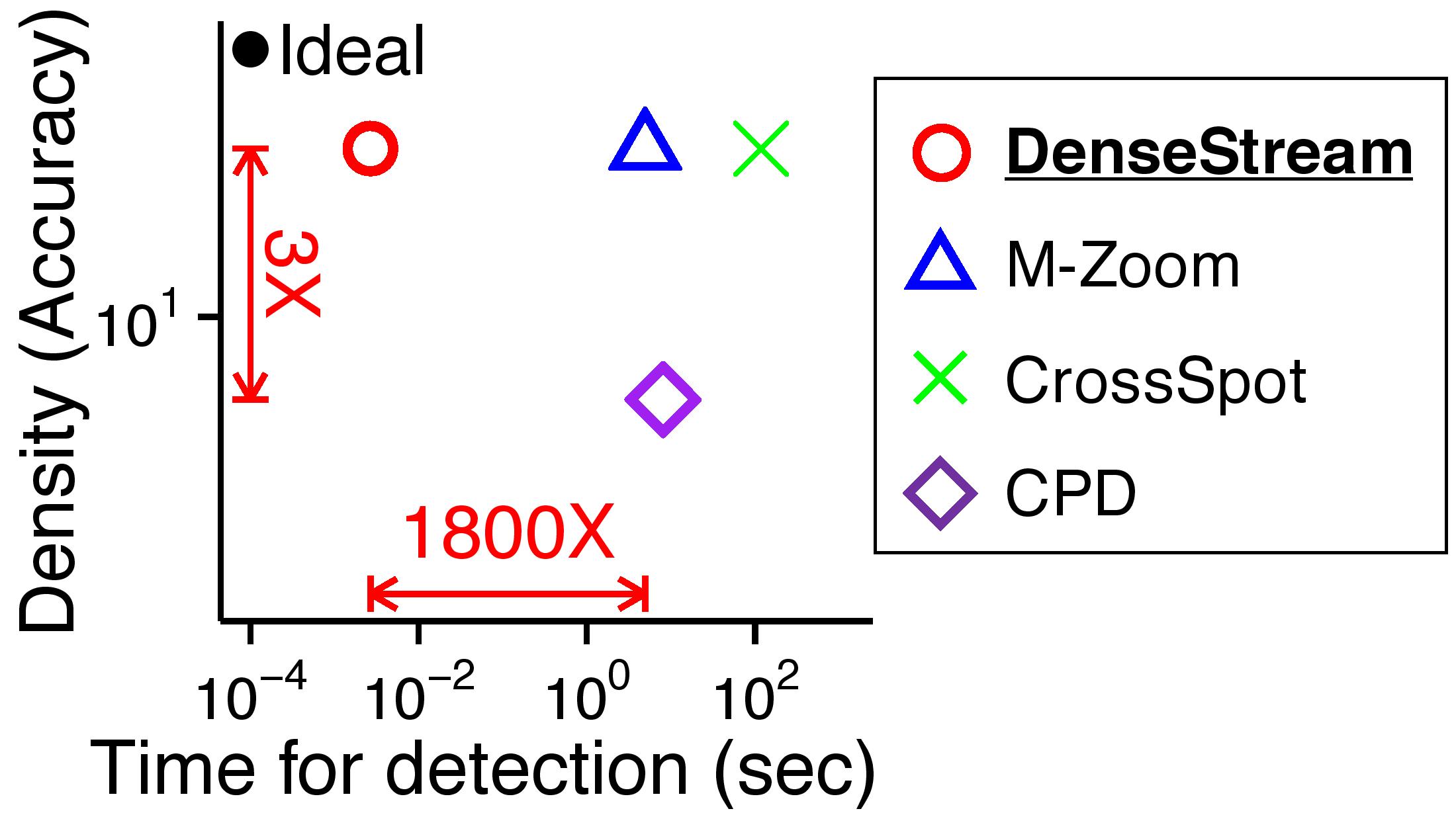
(a) Speed and accuracy of DenseStream

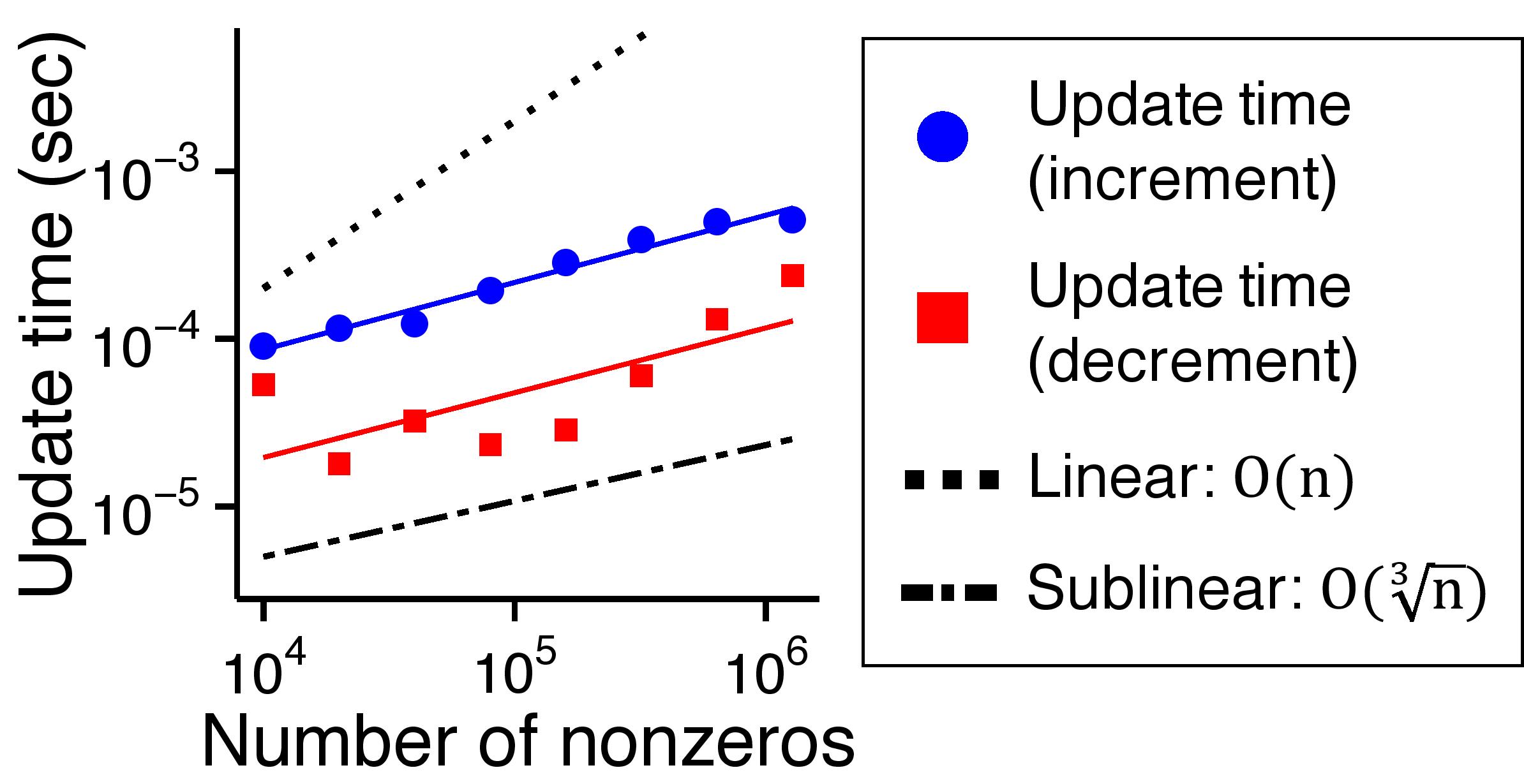
(b) Scalability of DenseStream

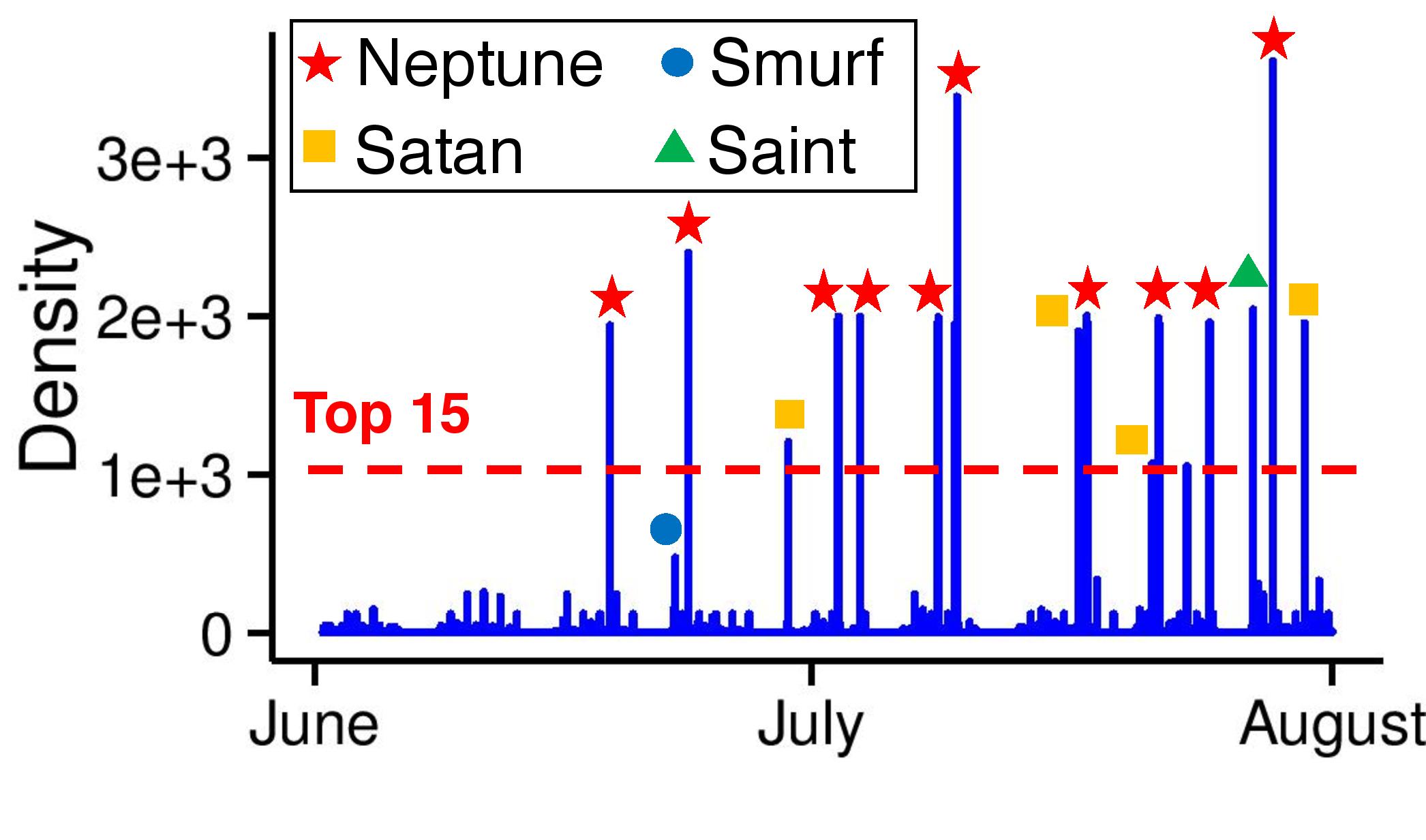
(c) Effectiveness of DenseAlert

Figure 1. Proposed algorithms are fast, accurate, scalable, and effective. (a) DenseStream, our incremental algorithm, detects dense subtensors significantly faster than batch algorithms without losing accuracy, as seen in the result in Yelp Dataset. (b) The time taken for each update in DenseStream grows sub-linearly with the size of data. (c) DenseAlert, which detects suddenly emerging dense subtensors, identifies network attacks from a TCP Dump with high accuracy (AUC=0.924). Especially, all the 15 densest subtensors revealed by DenseAlert indicate actual network attacks of various types.

Given a stream of changes in a tensor that evolves over time, how can we detect the sudden appearances of dense subtensors?

An important application of this problem is intrusion detection systems in networks, where attackers make a large number of connections to target machines to block their availability or to look for vulnerabilities (Lippmann et al., 2000). Consider a stream of connections where we represent each connection from a source IP address to a destination IP address as an entry in a 3-way tensor (source IP, destination IP, timestamp). Sudden appearances of dense subtensors in the tensor often indicate network attacks. For example, in Figure 1(c), all the top $15$ densest subtensors concentrated in a short period of time, which are detected by our DenseAlert algorithm, actually come from network attacks.

Table 1. Comparison of DenseStream, DenseAlert, and previous algorithms for detecting dense subtensors.

	M-Zoom (Shin et al., 2016b)	D-Cube (Shin et al., 2017)	CrossSpot (Jiang et al., 2015)	MAF (Maruhashi et al., 2011)	Fraudar (Hooi et al., 2016)	DenseStream	DenseAlert
Multi-Aspect Data	✓	✓	✓	✓		✓	✓
Accuracy Guarantees	✓	✓			✓	✓	✓
Incremental Updates						✓	✓
Slowly Formed Dense Subtensors	✓	✓	✓	✓	✓	✓
Small Sudden Dense Subtensors							✓

Another application is detecting fake rating attacks in review sites, such as Amazon and Yelp. Ratings can be modeled as entries in a 4-way tensor (user, item, timestamp, rating). Injection attacks maliciously manipulate the ratings of a set of items by adding a large number of similar ratings for the items, creating dense subtensors in the tensor. To guard against such fraud, an alert system detecting suddenly appearing dense subtensors in real time, as they arrive, is desirable.

Several algorithms for dense-subtensor detection have been proposed for detecting network attacks (Maruhashi et al., 2011; Shin et al., 2016b, 2017), retweet boosting (Jiang et al., 2015), rating attacks (Shin et al., 2017), and bots (Shin et al., 2016b) as well as for genetics applications (Saha et al., 2010). As summarized in Table 1, however, existing algorithms assume a static tensor rather than a stream of events (i.e., changes in a tensor) over time. In addition, our experiments in Section 4 show that they are limited in their ability to detect dense subtensors small but highly concentrated in a short period of time.

Our incremental algorithm DenseStream detects dense subtensors in real time as events arrive, and is hence more useful in many practical settings, including those mentioned above. DenseStream is also used as a building block of DenseAlert, an incremental algorithm for detecting the sudden emergences of dense subtensors. DenseAlert takes into account the tendency for lock-step behavior, such as network attacks and rating manipulation attacks, to appear within short, continuous intervals of time, which is an important signal for spotting lockstep behavior.

As the entries of a tensor change, our algorithms work by maintaining a small subset of subtensors that always includes a dense subtensor with a theoretical guarantee on its density. By focusing on this subset, our algorithms detect a dense subtensor in a time-evolving tensor up to a million times faster than the fastest batch algorithms, while providing the same theoretical guarantee on the density of the detected subtensor.

In summary, the main advantages of our algorithms are:

• Fast and ‘any time’: incremental updates by our algorithms are up to a million times faster than the fastest batch algorithms (Figure 1(a)).

• Provably accurate: our algorithms maintain a subtensor with a theoretical guarantee on its density, and in practice, its density is similar to that of subtensors found by the best batch algorithms (Figure 1(a)).

• Effective: DenseAlert successfully detects bot activities and network intrusions (Figure 1(c)) in real-world tensors. It also spots small-scale rating manipulation attacks, overlooked by existing algorithms.

Reproducibility: The code and data we used in the paper are available at http://www.cs.cmu.edu/~kijungs/codes/alert.

In Section 2, we introduce notations and problem definitions. In Section 3, we describe our proposed algorithms: DenseStream and DenseAlert. In Section 4, we present experimental results. After reviewing related work in Section 5, we conclude in Section 6.

2. Notations and Definitions

In this section, we introduce notations and concepts used in the paper. Then, we give formal problem definitions.

2.1. Notations and Concepts.

Symbols frequently used in the paper are listed in Table 2, and a toy example is in Example 2.1. We use $[y]=\{1,2...,y\}$ for brevity.

Table 2. Table of symbols.

Symbol	Definition
$\boldsymbol{\mathscr{T}}$	an input tensor
$N$	order of $\boldsymbol{\mathscr{T}}$
$t_{i_{1}...i_{N}}$	entry of $\boldsymbol{\mathscr{T}}$ with index $(i_{1},...,i_{N})$
$Q$	set of the slice indices of $\boldsymbol{\mathscr{T}}$
$q$	a member of $Q$
$\boldsymbol{\mathscr{T}}(S)$	subtensor composed of the slices in $S\subset Q$
$\pi:[|Q|]\rightarrow Q$	an ordering of slice indices in $Q$
$Q_{\pi,q}$	slice indices located after or equal to $q$ in $\pi$
$sum(\boldsymbol{\mathscr{T}}(S))$	sum of the entries included in $\boldsymbol{\mathscr{T}}(S)$
$d(\boldsymbol{\mathscr{T}}(S),q)$	slice sum of $q$ in $\boldsymbol{\mathscr{T}}(S)$
$d_{\pi}(q)$	slice sum of $q$ in $\boldsymbol{\mathscr{T}}(Q_{\pi,q})$
$c_{\pi}(q)$	cumulative max. slice sum of $q$ in $\boldsymbol{\mathscr{T}}(Q_{\pi,q})$
$((i_{1},...,i_{N}),\delta,+)$	increment of $t_{i_{1}...i_{N}}$ by $\delta$
$((i_{1},...,i_{N}),\delta,-)$	decrement of $t_{i_{1}...i_{N}}$ by $\delta$
$\rho(\boldsymbol{\mathscr{T}}(S))$	density of a subtensor $\boldsymbol{\mathscr{T}}(S)$
$\rho_{opt}$	density of the densest subtensor in $\boldsymbol{\mathscr{T}}$
$\Delta T$	time window in DenseAlert
$[y]$	$\{1,2...,y\}$

Notations for Tensors: Tensors are multi-dimensional arrays that generalize vectors (1-way tensors) and matrices (2-way tensors) to higher orders. Consider an $N$-way tensor $\boldsymbol{\mathscr{T}}$ of size $I_{1}\times...\times I_{N}$ with non-negative entries. Each $(i_{1},...,i_{N})$-th entry of $\boldsymbol{\mathscr{T}}$ is denoted by $t_{i_{1}...i_{N}}$. Equivalently, each $n$-mode index of $t_{i_{1}...i_{N}}$ is $i_{n}$. We use $\boldsymbol{\mathscr{T}}_{(n,i_{n})}$ to denote the $n$-mode slice (i.e. ($N-1$)-way tensor) obtained by fixing $n$-mode index to $i_{n}$. Then, $Q=\{(n,i_{n}):n\in[N],i_{n}\in[I_{n}]\}$ indicates all the slice indices. We denote a member of $Q$ by $q$.

For example, if $N=2$, $\boldsymbol{\mathscr{T}}$ is a matrix of size $I_{1}\times I_{2}$. Then, $\boldsymbol{\mathscr{T}}_{(1,i_{1})}$ is the $i_{1}$-th row of $\boldsymbol{\mathscr{T}}$, and $\boldsymbol{\mathscr{T}}_{(2,i_{2})}$ is the $i_{2}$-th column of $\boldsymbol{\mathscr{T}}$. In this setting, $Q$ is the set of all row and column indices.

Notations for Subtensors: Let $S$ be a subset of $Q$. $\boldsymbol{\mathscr{T}}(S)$ denotes the subtensor composed of the slices with indices in $S$, i.e., $\boldsymbol{\mathscr{T}}(S)$ is the subtensor left after removing all the slices with indices not in $S$.

For example, if $\boldsymbol{\mathscr{T}}$ is a matrix (i.e., $N=2$) and $S=\{(1,1),(1,2),$ $(2,2),(2,3)\}$, $\boldsymbol{\mathscr{T}}(S)$ is the submatrix of $\boldsymbol{\mathscr{T}}$ composed of the first and second rows and the second and third columns.

Notations for Orderings: Consider an ordering of the slice indices in $Q$. A function $\pi:[|Q|]\rightarrow Q$ denotes such an ordering where, for each $j\in[|Q|]$, $\pi(j)$ is the slice index in the $j$th position. That is, each slice index $q\in Q$ is in the $\pi^{-1}(q)$-th position in $\pi$. Let $Q_{\pi,q}=\{r\in Q:\pi^{-1}(r)\geq\pi^{-1}(q)\}$ be the slice indices located after or equal to $q$ in $\pi$. Then, $\boldsymbol{\mathscr{T}}(Q_{\pi,q})$ is the subtensor of $\boldsymbol{\mathscr{T}}$ composed of the slices with their indices in $Q_{\pi,q}$.

Notations for Slice Sum: We denote the sum of the entries of $\boldsymbol{\mathscr{T}}$ included in subtensor $\boldsymbol{\mathscr{T}}(S)$ by $sum(\boldsymbol{\mathscr{T}}(S))$. Similarly, we define the slice sum of $q\in Q$ in subtensor $\boldsymbol{\mathscr{T}}(S)$, denoted by $d(\boldsymbol{\mathscr{T}}(S),q)$, as the sum of the entries of $\boldsymbol{\mathscr{T}}$ that are included in both $\boldsymbol{\mathscr{T}}(S)$ and the slice with index $q\in Q$. For an ordering $\pi$ and a slice index $q\in Q$, we use $d_{\pi}(q)=d(\boldsymbol{\mathscr{T}}(Q_{\pi,q}),q)$ for brevity, and define the cumulative maximum slice sum of $q$ as $c_{\pi}(q)=\max\{d_{\pi}(r):r\in Q,\pi^{-1}(r)\leq\pi^{-1}(q)\}$, i.e., maximum $d_{\pi}(\cdot)$ among the slice indices located before or equal to $q$ in $\pi$.

Notations for Tensor Streams: A tensor stream is a sequence of changes in $\boldsymbol{\mathscr{T}}$. Let $((i_{1},...,i_{N}),\delta,+)$ be an increment of entry $t_{i_{1}...i_{N}}$ by $\delta>0$ and $((i_{1},...,i_{N}),\delta,-)$ be a decrement of entry $t_{i_{1}...i_{N}}$ by $\delta>0$.

Example 2.1 (Wikipedia Revision History).

Consider the $3$-way tensor in Figure 2. In the tensor, each entry $t_{ijk}$ indicates that user $i$ revised page $j$ on date $k$, $t_{ijk}$ times. The set of the slice indices is $Q=\{(1,1),(1,2),(1,3),(2,1),(2,2),(2,3),$ $(3,1),(3,2)\}$. Consider its subset $S=\{(1,1),(1,2),(2,1),$ $(2,2),(3,1)\}$. Then, $\boldsymbol{\mathscr{T}}(S)$ is the subtensor composed of the slices with their indices in $S$, as seen in Figure 2. In this setting, $sum(\boldsymbol{\mathscr{T}}(S))=4+5+7+3=19$, and $d(\boldsymbol{\mathscr{T}}(S),(2,2))=5+3=8$. Let $\pi$ be an ordering of $Q$ where $\pi(1)=(1,3)$, $\pi(2)=(2,3)$, $\pi(3)=(3,2)$, $\pi(4)=(2,2)$, $\pi(5)=(1,1)$, $\pi(6)=(1,2)$, $\pi(7)=(2,1)$, and $\pi(8)=(3,1)$. Then, $Q_{\pi,(2,2)}=S$, and $d_{\pi}((2,2))=d(\boldsymbol{\mathscr{T}}(Q_{\pi,(2,2)}),(2,2))=d(\boldsymbol{\mathscr{T}}(S),$ $(2,2))=8$.

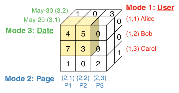
Figure 2. Pictorial depiction of Example 2.1. The colored region indicates subtensor $\boldsymbol{\mathscr{T}}(S)$.

2.2. Density Measure.

Definition 2.2 gives the density measure used in this work. That is, the density of a subtensor is defined as the sum of its entries divided by the number of the slices composing it. We let $\rho_{opt}$ be the density of the densest subtensor in $\boldsymbol{\mathscr{T}}$.

Definition 2.2.

(Density of a subtensor (Shin et al., 2016b)). Consider a subtensor $\boldsymbol{\mathscr{T}}(S)$ of a tensor $\boldsymbol{\mathscr{T}}$. The density of $\boldsymbol{\mathscr{T}}(S)$, which is denoted by $\rho(\boldsymbol{\mathscr{T}}(S))$, is defined as

$$\rho(\boldsymbol{\mathscr{T}}(S))=\frac{sum(\boldsymbol{\mathscr{T}}(S))}{|S|}.$$

This measure is chosen because: (a) it was successfully used for anomaly and fraud detection (Shin et al., 2016b, 2017), (b) this measure satisfies axioms that a reasonable “anomalousness” measure should meet (see Section A of the supplementary document (sup, 2017)), and (c) our algorithm based on this density measure outperforms existing algorithms based on different density measures in Section 4.5.1.

2.3. Problem Definitions.

We give the formal definitions of the problems studied in this work. The first problem (Problem 1) is to maintain the densest subtensor in a tensor that keeps changing.

Problem 1 (Detecting the Densest Subtensor in a Tensor Stream).

(1) Given: a sequence of changes in a tensor $\boldsymbol{\mathscr{T}}$ with slice indices $Q$ (i.e., a tensor stream) (2) maintain: a subtensor $\boldsymbol{\mathscr{T}}(S)$ where $S\subset Q$, (3) to maximize: its density $\rho(\boldsymbol{\mathscr{T}}(S))$.

Identifying the exact densest subtensor is computationally expensive even for a static tensor. For example, it takes $O(|Q|^{6})$ even when $\boldsymbol{\mathscr{T}}$ is a binary matrix (i.e., $N=2$) (Goldberg, 1984). Thus, we focus on designing an approximation algorithm that maintains a dense subtensor with a provable approximation bound, significantly faster than repeatedly finding a dense subtensor from scratch.

The second problem (Problem 2) is to detect suddenly emerging dense subtensors in a tensor stream. For a tensor $\boldsymbol{\mathscr{T}}$ whose values increase over time, let $\boldsymbol{\mathscr{T}}_{\Delta T}$ be the tensor where the value of each entry is the increment in the corresponding entry of $\boldsymbol{\mathscr{T}}$ in the last $\Delta T$ time units. Our aim is to spot dense subtensors appearing in $\boldsymbol{\mathscr{T}}_{\Delta T}$, which also keeps changing.

Problem 2 (Detecting Sudden Dense Subtensors in a Tensor Stream).

(1) Given: a sequence of increments in a tensor $\boldsymbol{\mathscr{T}}$ with slice indices $Q$ (i.e., a tensor stream) and a time window $\Delta T$, (2) maintain: a subtensor $\boldsymbol{\mathscr{T}}_{\Delta T}(S)$ where $S\subset Q$, (3) to maximize: its density $\rho(\boldsymbol{\mathscr{T}}_{\Delta T}(S))$.

3. Proposed Method

In this section, we propose DenseStream, which is an incremental algorithm for dense-subtensor detection in a tensor stream, and DenseAlert, which detects suddenly emerging dense subtensors. We first explain dense-subtensor detection in a static tensor in Section 3.1, then generalize this to DenseStream for a dynamic tensor in Section 3.2. Finally, we propose DenseAlert based on DenseStream in Section 3.3.

Algorithm 1 Dense-subtensor detection in a static tensor

1:a tensor $\boldsymbol{\mathscr{T}}$ with slice indices $Q$

2:a dense subtensor $\boldsymbol{\mathscr{T}}(S_{max})$

3:compute $\pi(\cdot)$, $d_{\pi}(\cdot)$, $c_{\pi}(\cdot)$ by D-ordering()

4:$S_{max}\leftarrow$ Find-Slices()

5:return $\boldsymbol{\mathscr{T}}(S_{max})$

6:procedure D-ordering():

7:$\vartriangleright$ find a D-ordering $\pi(\cdot)$ and compute $d_{\pi}(\cdot)$ and $c_{\pi}(\cdot)$

8:    $S\leftarrow Q$;  $c_{max}\leftarrow 0$ $\vartriangleright$ $c_{max}$: max. $d_{\pi}(\cdot)$ so far

9:    for $j\leftarrow 1...|Q|$ do

10:         $q\leftarrow\operatorname*{arg\,min}_{r\in S}d(\boldsymbol{\mathscr{T}}(S),r)$ $\vartriangleright$ $q$ has min. slice sum

11:         $\pi(j)\leftarrow q$ $\vartriangleright$ $S=Q_{\pi,q}$

12:         $d_{\pi}(q)\leftarrow d(\boldsymbol{\mathscr{T}}(S),q)$ $\vartriangleright$ $d_{\pi}(q)=d(\boldsymbol{\mathscr{T}}(Q_{\pi,q}),q)$

13:         $c_{\pi}(q)\leftarrow\max(c_{max},d_{\pi}(q))$;  $c_{max}\leftarrow c_{\pi}(q)$

14:         $S\leftarrow S/\{q\}$     

15:procedure Find-Slices():

16:$\vartriangleright$ find slices forming a dense subtensor from $\pi(\cdot)$ $d_{\pi}(\cdot)$, and $c_{\pi}(\cdot)$

17:    $S\leftarrow\emptyset$;  $m\leftarrow 0$; $\vartriangleright$ $m$: $sum(\boldsymbol{\mathscr{T}}(S))$

18:    $\rho_{max}\leftarrow-\infty$;  $q_{max}\leftarrow 0$ $\vartriangleright$ $\rho_{max}$: max. density so far

19:    for $j\leftarrow|Q|..1$ do

20:         $q\leftarrow\pi(j);\ S\leftarrow S\cup\{q\}$ $\vartriangleright$ $S=Q_{\pi,q}$

21:         $m\leftarrow m+d_{\pi}(q)$ $\vartriangleright$ $m=sum(\boldsymbol{\mathscr{T}}(Q_{\pi,q}))$

22:         if $m/|S|>\rho_{max}$ then

23:$\vartriangleright$ $m/|S|=\rho(\boldsymbol{\mathscr{T}}(Q_{\pi,q}))$

24:             $\rho_{max}\leftarrow m/|S|$;  $q_{max}\leftarrow q$              

25:    return $Q_{\pi,q_{max}}$ $\vartriangleright$ $q_{max}=\operatorname*{arg\,max}_{q\in Q}\rho(\boldsymbol{\mathscr{T}}(Q_{\pi,q}))$

3.1. Dense Subtensor Detection in Static Data.

We propose Algorithm 1 for detecting a dense subtensor in a static tensor. Although it eventually finds the same subtensor as M-Zoom (Shin et al., 2016b), Algorithm 1 also computes extra information, including a D-ordering (Definition 3.1), required for updating the subtensor in the following sections. Algorithm 1 has two parts: (a) D-ordering: find a D-ordering $\pi$ and compute $d_{\pi}(\cdot)$ and $c_{\pi}(\cdot)$; and (b) Find-Slices: find slices forming a dense subtensor from the result of (a).

Definition 3.1.

(D-ordering). An ordering $\pi$ is a D-ordering of $Q$ in $\boldsymbol{\mathscr{T}}$ if $\forall q\in Q$, $d(\boldsymbol{\mathscr{T}}(Q_{\pi,q}),q)=\min_{r\in Q_{\pi,q}}d(\boldsymbol{\mathscr{T}}(Q_{\pi,q}),r)$.

That is, a D-ordering is an ordering of slice indices obtained by choosing a slice index with minimum slice sum repeatedly, as in D-ordering() of Algorithm 1.

Using a D-ordering drastically reduces the search space while providing a guarantee on the accuracy. With a D-ordering $\pi$, Algorithm 1 reduces the search space of $2^{|Q|}$ possible subtensors to $\{\boldsymbol{\mathscr{T}}(Q_{\pi,q}):q\in Q\}$. In this space of size $|Q|$, however, there always exists a subtensor whose density is at least 1/(order of the input tensor) of maximum density, as formalized in Lemmas 3.2 and 3.3.

Lemma 3.2.

Let $\boldsymbol{\mathscr{T}}(S^{*})$ be a subtensor with the maximum density, i.e., $\rho(\boldsymbol{\mathscr{T}}(S^{*}))=\rho_{opt}$. Then for any $q\in S^{*}$,

(1) $$d(\boldsymbol{\mathscr{T}}(S^{*}),q)\geq\rho(\boldsymbol{\mathscr{T}}(S^{*})).$$

Proof. The maximality of the density of $\boldsymbol{\mathscr{T}}(S^{*})$ implies
$\rho(\boldsymbol{\mathscr{T}}(S^{*}\backslash\{q\}))\leq\rho(\boldsymbol{\mathscr{T}}(S^{*}))$, and plugging in Definition 2.2 to $\rho$ gives

$$\frac{sum(\boldsymbol{\mathscr{T}}(S^{*}))-d(\boldsymbol{\mathscr{T}}(S^{*}),q)}{|S^{*}|-1}=\frac{sum(\boldsymbol{\mathscr{T}}(S^{*}\backslash\{q\}))}{|S^{*}|-1}\\ =\rho(\boldsymbol{\mathscr{T}}(S^{*}\backslash\{q\}))\leq\rho(\boldsymbol{\mathscr{T}}(S^{*}))=\frac{sum(\boldsymbol{\mathscr{T}}(S^{*}))}{|S^{*}|},$$

which reduces to Eq. (1). ∎

Lemma 3.3.

Given a D-ordering $\pi$ in an $N$-way tensor $\boldsymbol{\mathscr{T}}$, there exists $q\in Q$ such that $\rho(\boldsymbol{\mathscr{T}}(Q_{\pi,q}))\geq\rho_{opt}/N$.
Proof. Let $\boldsymbol{\mathscr{T}}(S^{*})$ be satisfying $\rho(\boldsymbol{\mathscr{T}}(S^{*}))=\rho_{opt}$, and let $q^{*}\in S^{*}$ be satisfying that $\forall q\in S^{*}$, $\pi^{-1}(q^{*})\leq\pi^{-1}(q)$. Our goal is to show $\rho(\boldsymbol{\mathscr{T}}(Q_{\pi,q^{*}}))\geq\frac{1}{N}\rho(\boldsymbol{\mathscr{T}}(S^{*}))$, which we show as $N\rho(\boldsymbol{\mathscr{T}}(Q_{\pi,q^{*}}))\geq d(\boldsymbol{\mathscr{T}}(Q_{\pi,q^{*}}),q^{*})\geq d(\boldsymbol{\mathscr{T}}(S^{*}),q^{*})\geq\rho(\boldsymbol{\mathscr{T}}(S^{*}))$.

To show $N\rho(\boldsymbol{\mathscr{T}}(Q_{\pi,q^{*}}))\geq d(\boldsymbol{\mathscr{T}}(Q_{\pi,q^{*}}),q^{*})$, note $N\rho(\boldsymbol{\mathscr{T}}(Q_{\pi,q^{*}}))=\frac{sum(\boldsymbol{\mathscr{T}}(Q_{\pi,q^{*}}))N}{\left|Q_{\pi,q^{*}}\right|}$, and since $\boldsymbol{\mathscr{T}}$ is an $N$-way tensor, each entry is included in $N$ slices. Hence

(2) $$\sum\nolimits_{q\in Q_{\pi,q^{*}}}d(\boldsymbol{\mathscr{T}}(Q_{\pi,q^{*}}),q)=sum(\boldsymbol{\mathscr{T}}(Q_{\pi,q^{*}}))N.$$

Since $\pi$ is a $D$-ordering, $\forall q\in Q_{\pi,q^{*}}$, $d(\boldsymbol{\mathscr{T}}(Q_{\pi,q^{*}}),q)$ $\geq d(\boldsymbol{\mathscr{T}}(Q_{\pi,q^{*}}),q^{*})$ holds. Combining this and Eq. (2) gives

$$N\rho(\boldsymbol{\mathscr{T}}(Q_{\pi,q^{*}})) =\frac{sum(\boldsymbol{\mathscr{T}}(Q_{\pi,q^{*}}))N}{\left|Q_{\pi,q^{*}}\right|}$$

$$=\frac{\sum_{q\in Q_{\pi,q^{*}}}d(\boldsymbol{\mathscr{T}}(Q_{\pi,q^{*}}),q)}{\left|Q_{\pi,q^{*}}\right|}\geq d(\boldsymbol{\mathscr{T}}(Q_{\pi,q^{*}}),q^{*}).$$

Second, $d(\boldsymbol{\mathscr{T}}(Q_{\pi,q^{*}}),q^{*})\geq d(\boldsymbol{\mathscr{T}}(S^{*}),q^{*})$ is from that $S^{*}\subset Q_{\pi,q^{*}}$. Third, $d(\boldsymbol{\mathscr{T}}(S^{*}),q^{*})\geq\rho(\boldsymbol{\mathscr{T}}(S^{*}))$ is from Lemma 3.2. From these, $\rho(\boldsymbol{\mathscr{T}}(Q_{\pi,q^{*}}))\geq\frac{1}{N}\rho(\boldsymbol{\mathscr{T}}(S^{*}))$ holds. ∎

Such a subtensor $\boldsymbol{\mathscr{T}}(S_{max})$ is detected by Algorithm 1. That is, $\boldsymbol{\mathscr{T}}(S_{max})$ has density at least 1/(order of the input tensor) of maximum density, as proved in Theorem 3.4.

Theorem 3.4 (Accuracy Guarantee of Algorithm 1).

The subtensor returned by Algorithm 1 has density at least $\rho_{opt}/N$.
Proof. By Lemma 3.3, there exists a subtensor with density at least $\rho_{opt}/N$ among $\{\boldsymbol{\mathscr{T}}(Q_{\pi,q}):q\in Q\}$. The subtensor with the highest density in the set is returned by Algorithm 1. ∎

The time complexity of Algorithm 1 is linear with $nnz(\boldsymbol{\mathscr{T}})$, the number of the non-zero entries in $\boldsymbol{\mathscr{T}}$, as formalized in Theorem 3.6. Especially, finding $S_{max}$ takes only $O(|Q|)$ given $\pi(\cdot)$, $d_{\pi}(\cdot)$, and $c_{\pi}(\cdot)$, as shown in Lemma 3.5.

Lemma 3.5.

Let $S_{max}$ be the set of slice indices returned by Find-Slices() in Algorithm 1, and let $\boldsymbol{\mathscr{T}}(q)$ be the set of the non-zero entries in the slice with index $q$ in $\boldsymbol{\mathscr{T}}$. The time complexity of Find-Slices() in Algorithm 1 is $O(|Q|)$ and that of constructing $\boldsymbol{\mathscr{T}}(S_{max})$ from $S_{max}$ is $O(N|\bigcup_{q\in S_{max}}\boldsymbol{\mathscr{T}}(q)|)$.
Proof. Assume that, for each slice, the list of the non-zero entries in the slice is stored. In Find-Slices(), we iterate over the slices in $Q$, and each iteration takes $O(1)$. Thus, we get $O(|Q|)$. After finding $S_{max}$, in order to construct $\boldsymbol{\mathscr{T}}(S_{max})$, we have to process each non-zero entry included in any slice in $S_{max}$. The number of such entries is $|\bigcup_{q\in S_{max}}\boldsymbol{\mathscr{T}}(q)|$. Since processing each entry takes $O(N)$, constructing $\boldsymbol{\mathscr{T}}(S_{max})$ takes $O(N|\bigcup_{q\in S_{max}}\boldsymbol{\mathscr{T}}(q)|)$. ∎

Theorem 3.6 (Time Complexity of Algorithm 1).

The time complexity of Algorithm 1 is $O(|Q|\log|Q|+nnz(\boldsymbol{\mathscr{T}})N)$.
Proof. Assume that, for each slice, the list of the non-zero entries in the slice is stored. We first show that the time complexity of D-ordering() in Algorithm 1 is $O(|Q|\log|Q|+nnz(\boldsymbol{\mathscr{T}})N|)$. Assume we use a Fibonacci heap to find slices with minimum slice sum (line 10). Computing the slice sum of every slice takes $O(nnz(\boldsymbol{\mathscr{T}})N)$, and constructing a Fibonacci heap where each value is a slice index in $Q$ and the corresponding key is the slice sum of the slice takes $O(|Q|)$. Popping the index of a slice with minimum slice sum, which takes $O(\log|Q|)$, happens $|Q|$ times, and thus we get $O(|Q|\log|Q|)$. Whenever a slice index is popped we have to update the slice sums of its dependent slices (two slices are dependent if they have common non-zero entries). Updating the slice sum of each dependent slice, which takes $O(1)$ in a Fibonacci heap, happens at most $O(nnz(\boldsymbol{\mathscr{T}})N)$ times, and thus we get $O(nnz(\boldsymbol{\mathscr{T}})N)$. Their sum results in $O(|Q|\log|Q|+nnz(\boldsymbol{\mathscr{T}})N)$.

By Lemma 3.5, the time complexity of Find-Slices() is $O(|Q|)$, and that of constructing $\boldsymbol{\mathscr{T}}(S_{max})$ from $S_{max}$ is $O(N|\bigcup_{q\in S_{max}}\boldsymbol{\mathscr{T}}(q)|).$

Since the time complexity of D-ordering() dominates that of the remaining parts, we get $O(|Q|\log|Q|+nnz(\boldsymbol{\mathscr{T}})N)$ as the time complexity of Algorithm 1. ∎

3.2. DenseStream: Dense-Subtensor Detection in a Tensor Stream.

How can we update the subtensor found in Algorithm 1 under changes in the input tensor, rapidly, only when necessary, with the same approximation bound? For this purpose, we propose DenseStream, which updates the subtensor while satisfying Property 1. We explain the responses of DenseStream to increments of entry values (Section 3.2.1), decrements of entry values (Section 3.2.2), and changes of the size of the input tensor (Section 3.2.3).

Property 1 (Invariants in DenseStream).

For an $N$-way tensor $\boldsymbol{\mathscr{T}}$ that keeps changing, the ordering $\pi$ of the slice indices and the dense subtensor $\rho(\boldsymbol{\mathscr{T}}(S_{max}))$ maintained by DenseStream satisfy the following two conditions:

• $\pi$ is a D-ordering of $Q$ in $\boldsymbol{\mathscr{T}}$

• $\rho(\boldsymbol{\mathscr{T}}(S_{max}))$ $\geq\rho_{opt}/N$.

3.2.1. Increment of Entry Values.

Assume that the maintained dense subtensor $\boldsymbol{\mathscr{T}}(S_{max})$ and ordering $\pi$ (with $d_{\pi}(\cdot)$ and $c_{\pi}(\cdot)$) satisfy Property 1 in the current tensor $\boldsymbol{\mathscr{T}}$ (such $\pi$, $d_{\pi}(\cdot)$, $c_{\pi}(\cdot)$, and $\boldsymbol{\mathscr{T}}(S_{max})$ can be initialized by Algorithm 1 if we start from scratch). Algorithm 2 describes the response of DenseStream to $((i_{1},...,i_{N}),\delta,+)$, an increment of entry $t_{i_{1}...i_{N}}$ by $\delta>0$, for satisfying Property 1. Algorithm 2 has three steps: (a) Find-Region: find a region of the D-ordering $\pi$ that needs to be reordered, (b) Reorder: reorder the region obtained in (a), and (c) Update-Subtensor: use $\pi$ to rapidly update $\boldsymbol{\mathscr{T}}(S_{max})$ only when necessary. Each step is explained below.

(a) Find-Region (Line 7): The goal of this step is to find the region $[j_{L},j_{H}]\subset[1,|Q|]$ of the domain of the D-ordering $\pi$ that needs to be reordered in order for $\pi$ to remain as a D-ordering after the change $((i_{1},...,i_{N}),\delta,+)$. Let $C=\{(n,i_{n}):n\in[N]\}$ be the indices of the slices composing the changed entry $t_{i_{1}...i_{N}}$ and let $q_{f}=\operatorname*{arg\,min}_{q\in C}\pi^{-1}(q)$ be the one located first in $\pi$ among $C$. Then, let $M=\{q\in Q:\pi^{-1}(q)>\pi^{-1}(q_{f}),\ d_{\pi}(q)\geq d_{\pi}(q_{f})+\delta\}$ be the slice indices that are located after $q_{f}$ in $\pi$ among $Q$ and having $d_{\pi}(\cdot)$ at least $d_{\pi}(q_{f})+\delta$. Then, $j_{L}$ and $j_{H}$ are set as follows:

(3) $$j_{L}= \pi^{-1}(q_{f}),$$

(4) $$j_{H}= \begin{cases}\min_{q\in M}\pi^{-1}(q)-1&\text{if}\ M\neq\emptyset,\\ |Q|\text{ (i.e., the last index)}&\text{otherwise.}\end{cases}$$

Later in this section, we prove that slice indices whose locations do not belong to $[j_{L},j_{H}]$ need not be reordered by showing that there always exists a D-ordering $\pi^{\prime}$ in the updated $\boldsymbol{\mathscr{T}}$ where $\pi^{\prime}(j)=\pi(j)$ for every $j\notin[j_{L},j_{H}]$.

Algorithm 2 DenseStream in the case of increment

1:(1) current tensor: $\boldsymbol{\mathscr{T}}$ with slice indices $Q$

2:   (2) current dense subtensor: $\boldsymbol{\mathscr{T}}(S_{max})$ with Property 1

3:   (3) current D-ordering: $\pi(\cdot)$ (also $d_{\pi}(\cdot)$ and $c_{\pi}(\cdot)$)

4:   (4) a change in $\boldsymbol{\mathscr{T}}$: $((i_{1},...,i_{N}),\delta,+)$

5:updated dense subtensor $\boldsymbol{\mathscr{T}}(S_{max})$

6:$t_{i_{1}...i_{N}}\leftarrow t_{i_{1}...i_{N}}+\delta$

7:compute $j_{L}$ and $j_{H}$ by Eq. (3) and Eq. (4) $\vartriangleright$ [Find-Region]

8:compute $R$ by Eq. (5) $\vartriangleright$ [Reorder]

9:$S\leftarrow\{q\in Q:\pi^{-1}(q)\geq j_{L}\}$; $RS\leftarrow R\cap S$

10:$c_{max}\leftarrow 0$ $\vartriangleright$ $c_{max}$: max. $d_{\pi}(\cdot)$ so far

11:if $j_{L}>1$ then $c_{max}\leftarrow c_{\pi}(\pi(j_{L}-1))$

12:for $j\leftarrow j_{L}...j_{H}$ do

13:    $q\leftarrow\operatorname*{arg\,min}_{r\in RS}d(\boldsymbol{\mathscr{T}}(S),r)$ $\vartriangleright$ $q$ has min. slice sum

14:    $\pi(j)\leftarrow q$ $\vartriangleright$ by Lemma 3.7, $S=Q_{\pi,q}$, $RS=R\cap Q_{\pi,q}$

15:    $d_{\pi}(q)\leftarrow d(\boldsymbol{\mathscr{T}}(S),q)$ $\vartriangleright$ $d_{\pi}(q)=d(\boldsymbol{\mathscr{T}}(Q_{\pi,q}),q)$

16:    $c_{\pi}(q)\leftarrow\max(c_{max},d_{\pi}(q))$;  $c_{max}\leftarrow c_{\pi}(q)$

17:    $S\leftarrow S/\{q\}$; $RS\leftarrow RS/\{q\}$

18:if $c_{max}\geq\rho(\boldsymbol{\mathscr{T}}(S_{max}))$ then $\vartriangleright$ [Update-Subtensor]

19:    $S^{\prime}\leftarrow$Find-Slices() in Algorithm 1 $\vartriangleright$ time complexity: $O(|Q|)$

20:    if $S_{max}\neq S^{\prime}$ then $\boldsymbol{\mathscr{T}}(S_{max})\leftarrow\boldsymbol{\mathscr{T}}(S^{\prime})$     

21:return $\boldsymbol{\mathscr{T}}(S_{max})$

(b) Reorder (Lines 8-17): The goal of this step is to reorder the slice indices located in the region $[j_{L},j_{H}]$ so that $\pi$ remains as a D-ordering in $\boldsymbol{\mathscr{T}}$ after the change $((i_{1},...,i_{N}),\delta,+)$. Let $\boldsymbol{\mathscr{T}}^{\prime}$ be the updated $\boldsymbol{\mathscr{T}}$ and $\pi^{\prime}$ be the updated $\pi$ to distinguish them with $\boldsymbol{\mathscr{T}}$ and $\pi$ before the update. We get $\pi^{\prime}$ from $\pi$ by reordering the slice indices in

(5) $$R=\{q\in Q:\pi^{-1}(q)\in[j_{L},j_{H}]\}$$

so that the following condition is met for every $j\in[j_{L},j_{H}]$ and the corresponding $q=\pi^{\prime}(j)$:

(6) $$d(\boldsymbol{\mathscr{T}}^{\prime}(Q_{\pi^{\prime},q}),q)=\min\nolimits_{r\in R\cap Q_{\pi^{\prime},q}}d(\boldsymbol{\mathscr{T}}^{\prime}(Q_{\pi^{\prime},q}),r).$$

This guarantees that $\pi^{\prime}$ is a D-ordering in $\boldsymbol{\mathscr{T}}^{\prime}$, as shown in Lemma 3.7.

Lemma 3.7.

Let $\pi$ be a D-ordering in $\boldsymbol{\mathscr{T}}$, and let $\boldsymbol{\mathscr{T}}^{\prime}$ be $\boldsymbol{\mathscr{T}}$ after a change $((i_{1},...,i_{N}),\delta,+)$. For $R$ $(Eq.~{}\eqref{eq:increment:R})$ defined on $j_{L}$ and $j_{H}$ , $(Eq.~{}\eqref{eq:increment:min}$ and $Eq.~{}\eqref{eq:increment:max})$, let $\pi^{\prime}$ be an ordering of slice indices $Q$ where $\forall j\notin[j_{L},j_{H}],$ $\pi^{\prime}(j)=\pi(j)$ and $\forall j\in[j_{L},j_{H}]$, Eq. (6) holds. Then, $\pi^{\prime}$ is a D-ordering in $\boldsymbol{\mathscr{T}}^{\prime}$.
Proof. See Section B of the supplementary document (sup, 2017). ∎

(c) Update-Subtensor (Lines 18-20): In this step, we update the maintained dense subtensor $\boldsymbol{\mathscr{T}}(S_{max})$ when two conditions are met. We first check $c_{max}\geq\rho(\boldsymbol{\mathscr{T}}(S_{max}))$, which takes $O(1)$ if we maintain $\rho(\boldsymbol{\mathscr{T}}(S_{max}))$, since $c_{max}<\rho(\boldsymbol{\mathscr{T}}(S_{max}))$ entails that the updated entry $t_{i_{1}...i_{N}}$ is not in the densest subtensor (see the proof of Theorem 3.9 for details). We then check if there are changes in $S_{max}$, obtained by find-Slices(). This takes only $O(|Q|)$, as shown in Theorem 3.6. Even if both conditions are met, updating $\boldsymbol{\mathscr{T}}(S_{max})$ is simply to construct $\boldsymbol{\mathscr{T}}(S_{max})$ from given $S_{max}$ instead of finding $\boldsymbol{\mathscr{T}}(S_{max})$ from scratch. This conditional update reduces computation but still preserves Property 1, as formalized in Lemma 3.8 and Theorem 3.9.

Lemma 3.8.

Consider a D-ordering $\pi$ in $\boldsymbol{\mathscr{T}}$. For every entry $t_{i_{1}...i_{N}}$ with index $(i_{1},...,i_{N})$ belonging to the densest subtensor, $\forall n\in[N]$, $c_{\pi}((n,i_{n}))\geq\rho_{opt}$ holds.
Proof. Let $\boldsymbol{\mathscr{T}}(S^{*})$ be a subtensor with the maximum density, i.e., $\rho(\boldsymbol{\mathscr{T}}(S^{*}))=\rho_{opt}$. Let $q^{*}\in S^{*}$ be satisfying that $\forall q\in S^{*}$, $\pi^{-1}(q^{*})\leq\pi^{-1}(q)$. For any entry $t_{i_{1}...i_{N}}$ in $\boldsymbol{\mathscr{T}}(S^{*})$ with index $(i_{1},...,i_{N})$ and any $q\in\{(n,i_{n}):n\in[N]\}$, our goal is to show $c_{\pi}(q)\geq\rho(\boldsymbol{\mathscr{T}}(S^{*}))$, which we show as $c_{\pi}(q)\geq d_{\pi}(q^{*})\geq d(\boldsymbol{\mathscr{T}}(S^{*}),q^{*})$ $\geq\rho(\boldsymbol{\mathscr{T}}(S^{*}))$.

First, $c_{\pi}(q)\geq d_{\pi}(q^{*})$ is from the definition of $c_{\pi}(q)$ and $\pi^{-1}(q^{*})\leq\pi^{-1}(q)$. Second, from $S^{*}\subset Q_{\pi,q^{*}}$, $d_{\pi}(q^{*})=d(\boldsymbol{\mathscr{T}}(Q_{\pi,q^{*}}),$ $q^{*})\geq d(\boldsymbol{\mathscr{T}}(S^{*}),q^{*})$ holds. Third, $d(\boldsymbol{\mathscr{T}}(S^{*}),q^{*})\geq\rho(\boldsymbol{\mathscr{T}}(S^{*}))$ is from Lemma 3.2. From these, $c_{\pi}(q)\geq\rho(\boldsymbol{\mathscr{T}}(S^{*}))$ holds. ∎

Theorem 3.9 (Accuracy Guarantee of Algorithm 2).

Algorithm 2 preserves Property 1, and thus $\rho(\boldsymbol{\mathscr{T}}(S_{max}))\geq\rho_{opt}/N$ holds after Algorithm 2 terminates.
Proof. We assume that Property 1 holds and prove that it still holds after Algorithm 2 is executed. First, the ordering $\pi$ remains to be a D-ordering in $\boldsymbol{\mathscr{T}}$ by Lemma 3.7. Second, we show $\rho(\boldsymbol{\mathscr{T}}(S_{max}))$ $\geq\rho_{opt}/N$. If the condition in line 18 of Algorithm 2 is met, $\boldsymbol{\mathscr{T}}(S_{max})$ is set to the subtensor with the maximum density in $\{\boldsymbol{\mathscr{T}}(Q_{\pi,q}):q\in Q\}$ by Find-Slices(). By Lemma 3.3, $\rho(\boldsymbol{\mathscr{T}}(S_{max}))\geq\rho_{opt}/N$. If the condition in line 18 is not met, for the changed entry $t_{i_{1}...i_{N}}$ with index $(i_{1},...,i_{N})$, by the definition of $j_{L}$, there exists $n\in[N]$ such that $\pi(j_{L})=(n,i_{n})$. Since $j_{L}\leq j_{H}$, $c_{\pi}((n,i_{n}))=c_{\pi}(\pi(j_{L}))\leq c_{\pi}(\pi(j_{H}))=c_{max}<\rho(\boldsymbol{\mathscr{T}}(S_{max}))\leq\rho_{opt}$. Then, by Lemma 3.8, $t_{i_{1}...i_{N}}$ does not belong to the densest subtensor, which thus remains the same after the change $((i_{1},...,i_{N}),\delta,+)$. Since $\rho(\boldsymbol{\mathscr{T}}(S_{max}))$ never decreases, $\rho(\boldsymbol{\mathscr{T}}(S_{max}))$ $\geq\rho_{opt}/N$ still holds by Property 1, which we assume. Property 1 is preserved because its two conditions are met. ∎

Theorem 3.10 gives the time complexity of Algorithm 2. In the worst case (i.e., $R=Q$), this becomes $O(|Q|\log|Q|$ $+nnz(\boldsymbol{\mathscr{T}})N)$, which is the time complexity of Algorithm 1. In practice, however, $R$ is much smaller than $Q$, and updating $\boldsymbol{\mathscr{T}}(S_{max})$ happens rarely. Thus, in our experiments, Algorithm 2 scaled sub-linearly with $nnz(\boldsymbol{\mathscr{T}})$ (see Section 4.4).

Theorem 3.10 (Time Complexity of Algorithms 2 and 3).

Let $\boldsymbol{\mathscr{T}}(q)$ be the set of the non-zero entries in the slice with index $q$ in $\boldsymbol{\mathscr{T}}$. The time complexity of Algorithms 2 and 3 is $O(|R|\log|R|+|Q|+N|\bigcup_{q\in R}\boldsymbol{\mathscr{T}}(q)|+N|\bigcup_{q\in S_{max}}\boldsymbol{\mathscr{T}}(q)|)$.
Proof. Assume that, for each slice, the list of the non-zero entries in the slice is stored, and let $q_{f}=\pi(j_{L})$. Computing $j_{L}$, $j_{H}$, and $R$ takes $O(|R|)$. Assume we use a Fibonacci heap to find slices with minimum slice sum (line 13 of Algorithm 2). Computing the slice sum of every slice in $R$ in $\boldsymbol{\mathscr{T}}(Q_{\pi,q_{f}})$ takes $O(N|\bigcup_{q\in R}\boldsymbol{\mathscr{T}}(q)|)$. Then, constructing a Fibonacci heap where each value is a slice index in $R$ and the corresponding key is the slice sum of the slice in $\boldsymbol{\mathscr{T}}(Q_{\pi,q_{f}})$ takes $O(|R|)$. Popping the index of a slice with minimum slice sum, which takes $O(\log|R|)$, happens $|R|$ times, and thus we get $O(|R|\log|R|)$. Whenever a slice index is popped we have to update the slice sums of its dependent slices in $R$ (two slices are dependent if they have common non-zero entries). Updating the slice sum of each dependent slice, which takes $O(1)$ in a Fibonacci heap, happens at most $O(N|\bigcup_{q\in R}\boldsymbol{\mathscr{T}}(q)|)$ times, and thus we get $O(N|\bigcup_{q\in R}\boldsymbol{\mathscr{T}}(q)|)$. On the other hand, by Lemma 3.5, Find-Slices() and constructing $\boldsymbol{\mathscr{T}}(S_{max})$ from $S_{max}$ take $O(|Q|+N|\bigcup_{q\in S_{max}}\boldsymbol{\mathscr{T}}(q)|).$ Hence, the time complexity of Algorithms 2 and 3 is the sum of all the costs, which is $O(|R|\log|R|+|Q|+N|\bigcup_{q\in R}\boldsymbol{\mathscr{T}}(q)|+N|\bigcup_{q\in S_{max}}\boldsymbol{\mathscr{T}}(q)|)$. ∎

3.2.2. Decrement of Entry Values.

As in the previous section, assume that a tensor $\boldsymbol{\mathscr{T}}$, a D-ordering $\pi$ (also $d_{\pi}(\cdot)$ and $c_{\pi}(\cdot)$), and a dense subtensor $\boldsymbol{\mathscr{T}}(S_{max})$ satisfying Property 1 are maintained. (such $\pi$, $d_{\pi}(\cdot)$, $c_{\pi}(\cdot)$, and $\boldsymbol{\mathscr{T}}(S_{max})$ can be initialized by Algorithm 1 if we start from scratch). Algorithm 3 describes the response of DenseStream to $((i_{1},...,i_{N}),\delta,-)$, a decrement of entry $t_{i_{1}...i_{N}}$ by $\delta>0$, for satisfying Property 1. Algorithm 3 has the same structure of Algorithm 2, while they are different in the reordered region of $\pi$ and the conditions for updating the dense subtensor. The differences are explained below.

For a change $((i_{1},...,i_{N}),\delta,-)$, we find the region $[j_{L},j_{H}]$ of the domain of $\pi$ that may need to be reordered. Let $C=\{(n,i_{n}):n\in[N]\}$ be the indices of the slices composing the changed entry $t_{i_{1}...i_{N}}$, and let $q_{f}=\operatorname*{arg\,min}_{q\in C}\pi^{-1}(q)$ be the one located first in $\pi$ among $C$. Then, let $M_{min}=\{q\in Q:d_{\pi}(q)>c_{\pi}(q_{f})-\delta\}$ and $M_{max}=\{q\in Q:\pi^{-1}(q)>\pi^{-1}(q_{f}),\ d_{\pi}(q)\geq c_{\pi}(q_{f})\}$. Note that $M_{min}\neq\emptyset$ since, by the definition of $c_{\pi}(\cdot)$, there exists $q\in Q$ where $\pi^{-1}(q)\leq\pi^{-1}(q_{f})$ and $d_{\pi}(q)=c_{\pi}(q_{f})$. Then, $j_{L}$ and $j_{H}$ are:

(7) $$j_{L}= \min\nolimits_{q\in M_{min}}\pi^{-1}(q),$$

(8) $$j_{H}= \begin{cases}\min_{q\in M_{max}}\pi^{-1}(q)-1&\text{if}\ M_{max}\neq\emptyset,\\ |Q|\text{ (i.e., the last index)}&\text{otherwise.}\end{cases}$$

As in the increment case, we update $\pi$, to remain it as a D-ordering, by reordering the slice indices located in $[j_{L},j_{H}]$ of $\pi$. Let $\boldsymbol{\mathscr{T}}^{\prime}$ be the updated $\boldsymbol{\mathscr{T}}$ and $\pi^{\prime}$ be the updated $\pi$ to distinguish them with $\boldsymbol{\mathscr{T}}$ and $\pi$ before the update. Only the slice indices in $R=\{q\in Q:\pi^{-1}(q)\in[j_{L},j_{H}]\}$ are reordered in $\pi$ so that Eq. (6) is met for every $j\in[j_{L},j_{H}]$. This guarantees that $\pi^{\prime}$ is a D-ordering, as formalized in Lemma 3.11.

Algorithm 3 DenseStream in the case of decrement

1:(1) current tensor: $\boldsymbol{\mathscr{T}}$ with slice indices $Q$

2:   (2) current dense subtensor: $\boldsymbol{\mathscr{T}}(S_{max})$ with Property 1

3:   (3) current D-ordering: $\pi(\cdot)$ (also $c_{\pi}(\cdot)$ and $d_{\pi}(\cdot)$)

4:   (4) a change in $\boldsymbol{\mathscr{T}}$: $((i_{1},...,i_{N}),\delta,-)$

5:updated dense subtensor$\boldsymbol{\mathscr{T}}(S_{max})$

6:$t_{i_{1}...i_{N}}\leftarrow t_{i_{1}...i_{N}}-\delta$

7:compute $j_{L}$ and $j_{H}$ by Eq. (7) and (8) $\vartriangleright$ [Find-Region]

8:Lines 8-17 of Algorithm 2$\vartriangleright$ [Reorder]

9:if $t_{i_{1}...i_{N}}$ is in $\boldsymbol{\mathscr{T}}(S_{max})$ then $\vartriangleright$ [Update-Subtensor]

10:    $S^{\prime}\leftarrow$Find-Slices() in Algorithm 1 $\vartriangleright$ time complexity: $O(|Q|)$

11:    if $S_{max}\neq S^{\prime}$ then $\boldsymbol{\mathscr{T}}(S_{max})\leftarrow\boldsymbol{\mathscr{T}}(S^{\prime})$     

12:return $\boldsymbol{\mathscr{T}}(S_{max})$

Lemma 3.11.

Let $\pi$ be a D-ordering in $\boldsymbol{\mathscr{T}}$, and let $\boldsymbol{\mathscr{T}}^{\prime}$ be $\boldsymbol{\mathscr{T}}$ after a change $((i_{1},...,i_{N}),\delta,-)$. For $R$ $(Eq.~{}\eqref{eq:increment:R})$ defined on $j_{L}$ and $j_{H}$ $(Eq.~{}\eqref{eq:decrement:min}$ and $Eq.~{}\eqref{eq:decrement:max})$, let $\pi^{\prime}$ be an ordering of slice indices $Q$ where $\forall j\notin[j_{L},j_{H}],$ $\pi^{\prime}(j)=\pi(j)$ and $\forall j\in[j_{L},j_{H}]$, Eq. (6) holds. Then, $\pi^{\prime}$ is a D-ordering in $\boldsymbol{\mathscr{T}}^{\prime}$.
Proof. See Section B of the supplementary document (sup, 2017). ∎

The last step of Algorithm 3 is to conditionally and rapidly update the maintained dense subtensor $\boldsymbol{\mathscr{T}}(S_{max})$ using $\pi$. The subtensor $\boldsymbol{\mathscr{T}}(S_{max})$ is updated if entry $t_{i_{1}...i_{N}}$ belongs to $\boldsymbol{\mathscr{T}}(S_{max})$ (i.e., if $\rho(\boldsymbol{\mathscr{T}}(S_{max}))$ decreases by the change $((i_{1},...,i_{N}),\delta,-)$) and there are changes in $S_{max}$, obtained by find-Slices(). Checking these conditions takes only $O(|Q|)$, as in the increment case. Even if $\boldsymbol{\mathscr{T}}(S_{max})$ is updated, it is just constructing $\boldsymbol{\mathscr{T}}(S_{max})$ from given $S_{max}$, instead of finding $\boldsymbol{\mathscr{T}}(S_{max})$ from scratch.

Algorithm 3 preserves Property 1, as shown in Theorem 3.12, and has the same time complexity of Algorithm 2 in Theorem 3.10.

Theorem 3.12 (Accuracy Guarantee of Algorithm 3).

Algorithm 3 preserves Property 1. Thus, $\rho(\boldsymbol{\mathscr{T}}(S_{max}))\geq\rho_{opt}/N$ holds after Algorithm 3 terminates.
Proof. We assume that Property 1 holds and prove that it still holds after Algorithm 3 is executed. First, the ordering $\pi$ remains to be a D-ordering in $\boldsymbol{\mathscr{T}}$ by Lemma 3.11. Second, we show $\rho(\boldsymbol{\mathscr{T}}(S_{max}))\geq\rho_{opt}/N$. If the condition in line 9 of Algorithm 3 is met, $\boldsymbol{\mathscr{T}}(S_{max})$ is set to the subtensor with the maximum density in $\{\boldsymbol{\mathscr{T}}(Q_{\pi,q}):q\in Q\}$ by Find-Slices(). By Lemma 3.3, $\rho(\boldsymbol{\mathscr{T}}(S_{max}))\geq\rho_{opt}/N$. If the condition is not met, $\rho(\boldsymbol{\mathscr{T}}(S_{max}))$ remains the same, while $\rho_{opt}$ never increases. Hence, $\rho(\boldsymbol{\mathscr{T}}(S_{max}))\geq\rho_{opt}/N$ still holds by Property 1, which we assume. Since its two conditions are met, Property 1 is preserved. ∎

3.2.3. Increase or Decrease of Size.

DenseStream also supports the increase and decrease of the size of the input tensor. The increase of the size of $\boldsymbol{\mathscr{T}}$ corresponds to the addition of new slices to $\boldsymbol{\mathscr{T}}$. For example, if the length of the $n$th mode of $\boldsymbol{\mathscr{T}}$ increases from $I_{n}$ to $I_{n}+1$, the index $q=(n,I_{n}+1)$ of the new slice is added to $Q$ and the first position of $\pi$. We also set $d_{\pi}(q)$ and $c_{\pi}(q)$ to $0$. Then, if there exist non-zero entries in the new slice, they are handled one by one by Algorithm 2. Likewise, when size decreases, we first handle the removed non-zero entries one by one by Algorithm 3. Then, we remove the indices of the removed slices from $Q$ and $\pi$.

3.3. DenseAlert: Suddenly Emerging Dense-Subtensor Detection

Based on DenseStream, we propose DenseAlert, an incremental algorithm for detecting suddenly emerging dense subtensors. For a stream of increments in the input tensor $\boldsymbol{\mathscr{T}}$, DenseAlert maintains $\boldsymbol{\mathscr{T}}_{\Delta T}$, a tensor where the value of each entry is the increment of the value of the corresponding entry in $\boldsymbol{\mathscr{T}}$ in last $\Delta T$ time units (see Problem 2 in Section 2.3), as described in Figure 3 and Algorithm 4, To maintain $\boldsymbol{\mathscr{T}}_{\Delta T}$ and a dense subtensor in it, DenseAlert applies increments by DenseStream (line 7), and undoes the increments after $\Delta T$ time units also by DenseStream (lines 8 and 10). The accuracy of DenseAlert, formalized in Theorem 3.13, is implied from the accuracy of DenseStream.

Figure 3. DenseAlert with Wikipedia Revision History (Example 2.1). DenseAlert (yellow box in the figure) spots dense subtensors formed within $\Delta T$ time units.

Algorithm 4 DenseAlert for sudden dense subtensors

1:(1) sequence of increments in $\boldsymbol{\mathscr{T}}$

2:   (2) time window: $\Delta T$

3:suddenly emerging dense subtensors

4:run Algorithm 1 with a zero tensor

5:wait until the next change happens at time $T$

6:if the change is $((i_{1},...,i_{N}),\delta,+)$ then

7:    run DenseStream (Algorithm 2)

8:    schedule $((i_{1},...,i_{N}),\delta,-)$ at time $T+\Delta T$

9:else if the change is $((i_{1},...,i_{N}),\delta,-)$ then

10:    run DenseStream (Algorithm 3)

11:report the current dense subtensor

12:goto Line 2

Theorem 3.13 (Accuracy Guarantee of Algorithm 4).

Let $\Delta\rho_{opt}$ be the density of the densest subtensor in the $N$-way tensor $\boldsymbol{\mathscr{T}}_{\Delta T}$. The subtensor maintained by Algorithm 4 has density at least $\Delta\rho_{opt}/N$.
Proof. By Theorems 3.9 and 3.12, DenseAlert, which uses DenseStream for updates, maintains a subtensor with density at least $1/N$ of the density of the densest subtensor. ∎

The time complexity of DenseAlert is also obtained from Theorem 3.10 by simply replacing $\boldsymbol{\mathscr{T}}$ with $\boldsymbol{\mathscr{T}}_{\Delta T}$. DenseAlert needs to store only $\boldsymbol{\mathscr{T}}_{\Delta T}$ (i.e., the changes in the last $\Delta T$ units) in memory at a time. DenseAlert discards older changes.

4. Experiments

Table 3. Summary of real-world tensor datasets.

Name	Size	$\mathbf{|Q|}$	$\mathbf{nnz(\boldsymbol{\mathscr{T}})}$
Ratings: users $\times$ items $\times$ timestamps $\times$ ratings $\rightarrow$ #reviews
Yelp (dat, 2017)	552K $\times$ 77.1K $\times$ 3.80K $\times$ 5	633K	2.23M
Android (McAuley et al., 2015)	1.32M $\times$ 61.3K $\times$ 1.28K $\times$ 5	1.39M	2.64M
YahooM. (Dror et al., 2012)	1.00M $\times$ 625K $\times$ 84.4K $\times$ 101	1.71M	253M
Wikipedia edit history: users $\times$ pages $\times$ timestamps $\rightarrow$ #edits
KoWiki (Shin et al., 2016b)	470K $\times$ 1.18M $\times$ 101K	1.80M	11.0M
EnWiki (Shin et al., 2016b)	44.1M $\times$ 38.5M $\times$ 129K	82.8M	483M
Social networks: users $\times$ users $\times$ timestamps $\rightarrow$ #interactions
Youtube (Mislove et al., 2007)	3.22M $\times$ 3.22M $\times$ 203	6.45M	18.7M
SMS	1.25M $\times$ 7.00M $\times$ 4.39K	8.26M	103M
TCP dumps: IPs $\times$ IPs $\times$ timestamps $\rightarrow$ #connections
TCP (Lippmann et al., 2000)	9.48K $\times$ 23.4K $\times$ 46.6K	79.5K	522K

We design experiments to answer the following questions:

• Q1. Speed: How fast are updates in DenseStream compared to batch algorithms?

• Q2. Accuracy: How accurately does DenseStream maintain a dense subtensor?

• Q3. Scalability: How does the running time of DenseStream increase as input tensors grow?

• Q4. Effectiveness: Which anomalies or fraudsters does DenseAlert spot in real-world tensors?

4.1. Experimental Settings.

Machine: We ran all experiments on a machine with 2.67GHz Intel Xeon E7-8837 CPUs and 1TB memory (up to 85GB was used by our algorithms).

Data: Table 3 lists the real-world tensors used in our experiments. Ratings are 4-way tensors (users, items, timestamps, ratings) where entry values are the number of reviews. Wikipedia edit history is 3-way tensors (users, pages, timestamps) where entry values are the number of edits. Social networks are 3-way tensors (source users, destination users, timestamps) where entry values are the number of interactions. TCP dumps are 3-way tensors (source IPs, destination IPs, timestamps) where entry values are the number of TCP connections. Timestamps are in dates in Yelp and Youtube, in minutes in TCP, and in hours in the others.

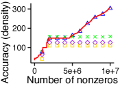
(a) SMS (part)

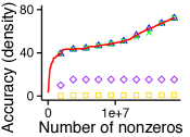
(b) Youtube

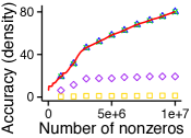
(c) EnWiki (part)

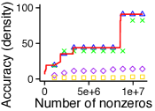
(d) KoWiki

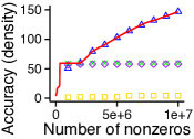
(e) YahooM. (part)

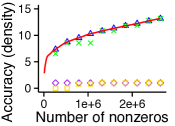
(f) Android

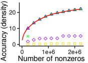
(g) Yelp

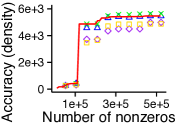
(h) TCP

Figure 4. DenseStream is ‘any-time’ and accurate. While tensors grow, DenseStream maintains and instantly updates a dense subtensor, whereas batch algorithms update dense subtensors only once in a time interval. Subtensors maintained by DenseStream have density (red lines) similar to the density (points) of the subtensors found by the best batch algorithms.

Implementations: We implemented dense-subtensor detection algorithms for comparison. We implemented our algorithms, M-Zoom (Shin et al., 2016b), and CrossSpot (Jiang et al., 2015) in Java, while we used Tensor Toolbox (Bader et al., 2017) for CP decomposition (CPD) and MAF (Maruhashi et al., 2011). In all the implementations, a sparse tensor format was used so that the space usage is proportional to the number of non-zero entries. As in (Shin et al., 2016b), we used a variant of CrossSpot which maximizes the density measure defined in Definition 2.2 and uses CPD for seed selection. For each batch algorithm, we reported the densest one after finding three dense subtensors.

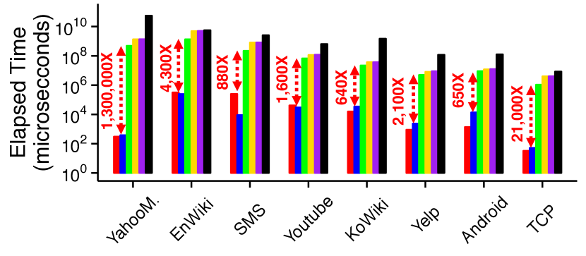
Figure 5. DenseStream outperforms batch algorithms. An update in DenseStream was up to a million times faster than the fastest batch algorithm.

4.2. Q1. Speed

We show that updating a dense subtensor by DenseStream is significantly faster than running batch algorithms from scratch. For each tensor stream, we averaged the update times for processing the last 10,000 changes corresponding to increments (blue bars in Figure 5). Likewise, we averaged the update times for undoing the first 10,000 increments, i.e., decreasing the values of the oldest entries (red bars in Figure 5). Then, we compared them to the time taken for running batch algorithms on the final tensor that each tensor stream results in. As seen in Figure 5, updates in DenseStream were up to a million times faster than the fastest batch algorithm. The speed-up was particularly high in sparse tensors having a widespread slice sum distribution (thus having a small reordered region $R$), as we can expect from Theorem 3.10.

On the other hand, the update time in DenseAlert, which uses DenseStream as a sub-procedure, was similar to that in DenseStream when the time interval $\Delta T=\infty$, and was less with smaller $\Delta T$. This is since the average number of non-zero entries maintained is proportional to $\Delta T$.

4.3. Q2. Accuracy

This experiment demonstrates the accuracy of DenseStream. From this, the accuracy of DenseAlert, which uses DenseStream as a sub-procedure, is also obtained. We tracked the density of the dense subtensor maintained by DenseStream while each tensor grows, and compared it to the densities of the dense subtensors found by batch algorithms. As seen in Figure 4, the subtensors that DenseStream maintained had density (red lines) similar to the density (points) of the subtensors found by the best batch algorithms. Moreover, DenseStream is ‘any time’; that is, as seen in Figure 4, DenseStream updates the dense subtensor instantly, while the batch algorithms cannot update their dense subtensors until the next batch processes end. DenseStream also maintains a dense subtensor accurately when the values of entries decrease, as shown in Section C of the supplementary document (sup, 2017).

The accuracy and speed (measured in Section 4.2) of the algorithms in Yelp Dataset are shown in Figure 1(a) in Section 1. DenseStream significantly reduces the time gap between the emergence and the detection of a dense subtensor, without losing accuracy.

4.4. Q3. Scalability

We demonstrate the high scalability of DenseStream by measuring how rapidly its update time increases as a tensor grows. For this experiment, we used a $10^{5}\times 10^{5}\times 10^{5}$ random tensor stream that has a realistic power-law slice sum distribution in each mode. As seen in Figure 1(b) in Section 1, update times, for both types of changes, scaled sub-linearly with the number of nonzero entries. Note that DenseAlert, which uses DenseStream as a sub-procedure, has the same scalability.

4.5. Q4. Effectiveness

In this section, we show the effectiveness of DenseAlert in practice. We focus on DenseAlert, which spots suddenly emerging dense subtensors overlooked by existing methods, rather than DenseStream, which is much faster but eventually finds a similar subtensor with previous algorithms, especially (Shin et al., 2016b).

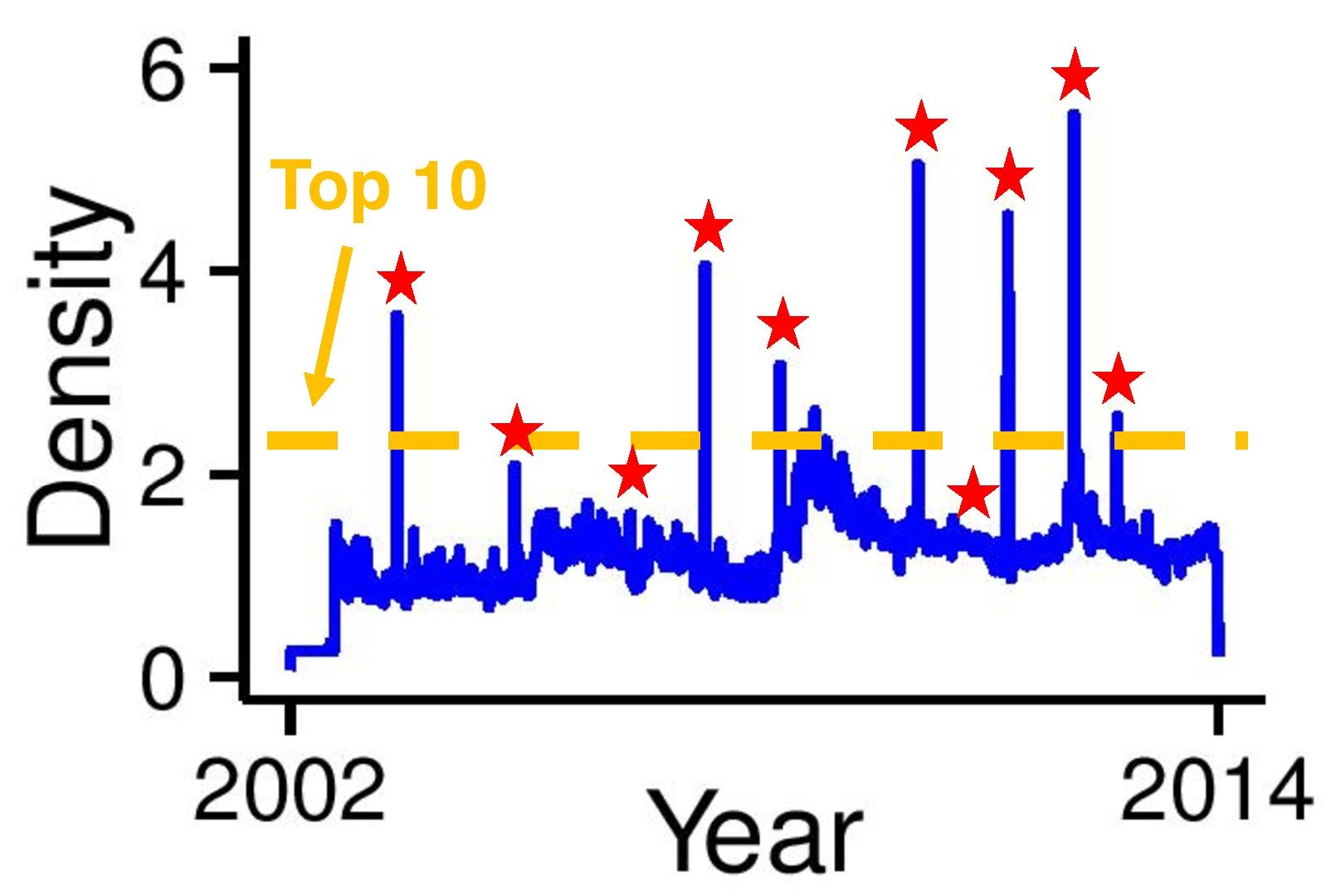
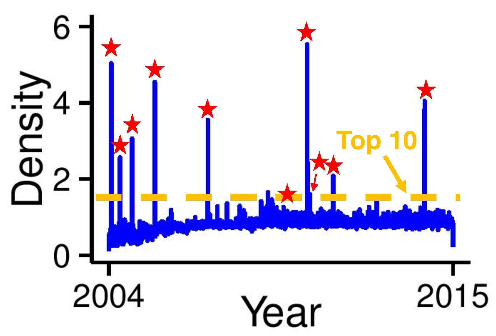
(a) DenseAlert in Yelp (left) and Android (right)

[0pt 4pt] Recall @ Top-10 Recall @ Top-10 in Yelp in Android DenseAlert 0.9 0.7 Others (Hooi et al., 2016; Jiang et al., 2015; Maruhashi et al., 2011; Shin et al., 2016b, 2017) 0.0 0.0

(b) Comparison with other anomaly detection algorithms

Figure 6. DenseAlert accurately detects small-scale short- period attacks injected in review datasets. However, these attacks are overlooked by existing methods.

4.5.1. Small-scale Attack Detection in Ratings.

For rating datasets, where ground-truth labels are unavailable, we assume an attack scenario where fraudsters in a rating site, such as Yelp, utilize multiple user accounts and give the same rating to the same set of items (or businesses) in a short period of time. The goal of the fraudsters is to boost (or lower) the ratings of the items rapidly. This lockstep behavior results in a dense subtensor of size $\#fake\_accounts\times\#target\_items\times 1\times 1$ in rating datasets whose modes are users, items, timestamps, and ratings. Here, we assume that fraudsters are not blatant but careful enough to adjust their behavior so that only small-scale dense subtensors are formed.

We injected $10$ such small random dense subtensors of sizes from $3\times 3\times 1\times 1$ to $12\times 12\times 1\times 1$ in Yelp and Android datasets, and compared how many of them are detected by each anomaly-detection algorithm. As seen in Figure 6(a), DenseAlert (with $\Delta T$=1 time unit in each dataset) clearly revealed the injected subtensors. Specifically, 9 and 7 among the top $10$ densest subtensors spotted by DenseAlert indeed indicate the injected attacks in Yelp and Android datasets, respectively. However, the injected subtensors were not revealed when we simply investigated the number of ratings in each time unit. Moreover, as summarized in Figure 6(b), none of the injected subtensors was detected by existing algorithms (Hooi et al., 2016; Jiang et al., 2015; Maruhashi et al., 2011; Shin et al., 2016b). These existing algorithms failed since they either ignore time information (Hooi et al., 2016) or only find dense subtensors in the entire tensor (Jiang et al., 2015; Maruhashi et al., 2011; Shin et al., 2016b, 2017) without using a time window.

4.5.2. Network Intrusion Detection.

Figure 1(c) shows the changes of the density of the maintained dense subtensor when we applied DenseAlert to TCP Dataset with the time window $\Delta T$ = 1 minute. We found out that the sudden emergence of dense subtensors (i.e., sudden increase in the density) indicates network attacks of various types. Especially, according to the ground-truth labels, all top 15 densest subtensors correspond to actual network attacks. Classifying each connection as an attack or a normal connection based on the density of the densest subtensor including the connection (i.e., the denser subtensor including a connection is, the more suspicious the connection is) led to high accuracy with AUC (Area Under the Curve) 0.924. This was better than MAF (0.514) and comparable with CPD (0.926), CrossSpot (0.923), and M-Zoom (0.921). The result is still noteworthy since DenseAlert requires only changes in the input tensor within $\Delta T$ time units at a time, while the others require the entire tensor at once.

4.5.3. Anomaly Detection in Wikipedia.

The sudden appearances of dense subtensors also signal anomalies in Wikipedia edit history. Figure 7 depicts the changes of the density of the dense subtensor maintained by DenseAlert in KoWiki Dataset with the time window $\Delta T$ = 24 hours. We investigated the detected dense subtensors and found out that most of them corresponded to actual anomalies including edit wars, bot activities, and vandalism. For example, the densest subtensor, composed by three users and two pages, indicated an edit war where three users edited two pages about regional prejudice 900 times within a day.

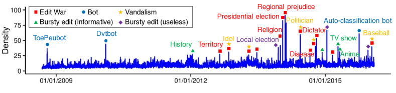
Figure 7. DenseAlert successfully spots anomalies in Korean Wikipedia. The sudden appearances of dense subtensors signal actual anomalies of various types including edit wars, bot activities, and vandalism. The densest subtensor indicates an edit war where three users edited two pages about regional prejudice 900 times within a day.

5. Related Work

Dense Subgraph Detection. For densest-subgraph detection in unweighted graphs, max-flow-based exact algorithms (Goldberg, 1984; Khuller and Saha, 2009) and greedy approximation algorithms (Charikar, 2000; Khuller and Saha, 2009) have been proposed. Extensions include adding size bounds (Andersen and Chellapilla, 2009), using alternative metrics (Tsourakakis et al., 2013), finding subgraphs with limited overlap (Balalau et al., 2015; Galbrun et al., 2016), and extending to large-scale graphs (Bahmani et al., 2012, 2014) and dynamic graphs (Epasto et al., 2015; McGregor et al., 2015; Bhattacharya et al., 2015). Other approaches include spectral methods (Prakash et al., 2010) and frequent itemset mining (Seppänen and Mannila, 2004). Dense-subgraph detection has been widely used to detect fraud or spam in social and review networks (Jiang et al., 2014; Beutel et al., 2013; Shah et al., 2014; Hooi et al., 2016; Shin et al., 2016a).

Dense Subtensor Detection. To incorporate additional dimensions and identify lockstep behavior with greater specificity, dense-subtensor detection in multi-aspect data (i.e., tensors) has been considered. Especially, a likelihood-based approach called CrossSpot (Jiang et al., 2015) and a greedy approach giving an accuracy guarantee called M-Zoom (Shin et al., 2016b) were proposed for this purpose. M-Zoom was also extended for large datasets stored on a disk or on a distributed file system (Shin et al., 2017). Dense-subtensor detection has been used for network-intrusion detection (Maruhashi et al., 2011; Shin et al., 2016b, 2017), retweet-boosting detection (Jiang et al., 2015), bot detection (Shin et al., 2016b), rating-attack detection (Shin et al., 2017), genetics applications (Saha et al., 2010), and formal concept mining (Cerf et al., 2008; Ignatov et al., 2013). However, these existing approaches assume a static tensor rather than a stream of events over time, and do not detect dense subtensors in real time, as they arrive. We also show their limitations in detecting dense subtensors small but highly concentrated in a short period of time.

Tensor Decomposition. Tensor decomposition such as HOSVD and CPD (Kolda and Bader, 2009) can be used to find dense subtensors in tensors, as MAF (Maruhashi et al., 2011) uses CPD for detecting anomalous subgraph patterns in heterogeneous networks. Streaming algorithms (Sun et al., 2006; Zhou et al., 2016) also have been developed for CPD and Tucker Decomposition. However, dense-subtensor detection based on tensor decomposition showed limited accuracy in our experiments (see Section 4.3).

6. Conclusion

In this work, we propose DenseStream, an incremental algorithm for detecting a dense subtensor in a tensor stream, and DenseAlert, an incremental algorithm for spotting the sudden appearances of dense subtensors. They have the following advantages:

• Fast and ‘any time’: our algorithms maintain and update a dense subtensor in a tensor stream, which is up to a million times faster than batch algorithms (Figure 5).

• Provably accurate: The densities of subtensors maintained by our algorithms have provable lower bounds (Theorems 3.9, 3.12, 3.13) and are high in practice (Figure 4).

• Effective: DenseAlert successfully detects anomalies, including small-scale attacks, which existing algorithms overlook, in real-world tensors (Figures 6 and 7).

Reproducibility: The code and data used in the paper are available at http://www.cs.cmu.edu/~kijungs/codes/alert.

References

- (1)
- sup (2017) 2017. Supplementary Document. Available online: http://www.cs.cmu.edu/~kijungs/codes/alert/supple.pdf.
- dat (2017) 2017. Yelp Dataset Challenge. https://www.yelp.com/dataset_challenge. https://www.yelp.com/dataset_challenge
- Andersen and Chellapilla (2009) Reid Andersen and Kumar Chellapilla. 2009. Finding dense subgraphs with size bounds. In WAW.
- Bader et al. (2017) Brett W. Bader, Tamara G. Kolda, et al. 2017. MATLAB Tensor Toolbox Version 2.6. Available online. (2017). http://www.sandia.gov/~tgkolda/TensorToolbox/
- Bahmani et al. (2014) Bahman Bahmani, Ashish Goel, and Kamesh Munagala. 2014. Efficient primal-dual graph algorithms for mapreduce. In WAW.
- Bahmani et al. (2012) Bahman Bahmani, Ravi Kumar, and Sergei Vassilvitskii. 2012. Densest subgraph in streaming and mapreduce. PVLDB 5, 5 (2012), 454–465.
- Balalau et al. (2015) Oana Denisa Balalau, Francesco Bonchi, TH Chan, Francesco Gullo, and Mauro Sozio. 2015. Finding subgraphs with maximum total density and limited overlap. In WSDM.
- Beutel et al. (2013) Alex Beutel, Wanhong Xu, Venkatesan Guruswami, Christopher Palow, and Christos Faloutsos. 2013. Copycatch: stopping group attacks by spotting lockstep behavior in social networks. In WWW.
- Bhattacharya et al. (2015) Sayan Bhattacharya, Monika Henzinger, Danupon Nanongkai, and Charalampos Tsourakakis. 2015. Space-and time-efficient algorithm for maintaining dense subgraphs on one-pass dynamic streams. In STOC.
- Cerf et al. (2008) Loïc Cerf, Jérémy Besson, Céline Robardet, and Jean-François Boulicaut. 2008. Data Peeler: Contraint-Based Closed Pattern Mining in n-ary Relations.. In SDM.
- Charikar (2000) Moses Charikar. 2000. Greedy approximation algorithms for finding dense components in a graph. In APPROX.
- Dror et al. (2012) Gideon Dror, Noam Koenigstein, Yehuda Koren, and Markus Weimer. 2012. The Yahoo! Music Dataset and KDD-Cup’11. In KDD Cup.
- Epasto et al. (2015) Alessandro Epasto, Silvio Lattanzi, and Mauro Sozio. 2015. Efficient densest subgraph computation in evolving graphs. In WWW.
- Galbrun et al. (2016) Esther Galbrun, Aristides Gionis, and Nikolaj Tatti. 2016. Top-k overlapping densest subgraphs. Data Mining and Knowledge Discovery (2016), 1–32.
- Goldberg (1984) Andrew V Goldberg. 1984. Finding a maximum density subgraph. Technical Report.
- Hooi et al. (2016) Bryan Hooi, Hyun Ah Song, Alex Beutel, Neil Shah, Kijung Shin, and Christos Faloutsos. 2016. FRAUDAR: Bounding Graph Fraud in the Face of Camouflage. In KDD.
- Ignatov et al. (2013) Dmitry I Ignatov, Sergei O Kuznetsov, Jonas Poelmans, and Leonid E Zhukov. 2013. Can triconcepts become triclusters? Int. J. General Systems 42, 6 (2013), 572–593.
- Jiang et al. (2015) Meng Jiang, Alex Beutel, Peng Cui, Bryan Hooi, Shiqiang Yang, and Christos Faloutsos. 2015. A general suspiciousness metric for dense blocks in multimodal data. In ICDM.
- Jiang et al. (2014) Meng Jiang, Peng Cui, Alex Beutel, Christos Faloutsos, and Shiqiang Yang. 2014. Catchsync: catching synchronized behavior in large directed graphs. In KDD.
- Khuller and Saha (2009) Samir Khuller and Barna Saha. 2009. On finding dense subgraphs. In ICALP.
- Kolda and Bader (2009) Tamara G Kolda and Brett W Bader. 2009. Tensor decompositions and applications. SIAM review 51, 3 (2009), 455–500.
- Lippmann et al. (2000) Richard P Lippmann, David J Fried, Isaac Graf, Joshua W Haines, Kristopher R Kendall, David McClung, Dan Weber, Seth E Webster, Dan Wyschogrod, Robert K Cunningham, et al. 2000. Evaluating intrusion detection systems: The 1998 DARPA off-line intrusion detection evaluation. In DISCEX.
- Maruhashi et al. (2011) Koji Maruhashi, Fan Guo, and Christos Faloutsos. 2011. Multiaspectforensics: Pattern mining on large-scale heterogeneous networks with tensor analysis. In ASONAM.
- McAuley et al. (2015) Julian McAuley, Rahul Pandey, and Jure Leskovec. 2015. Inferring networks of substitutable and complementary products. In KDD.
- McGregor et al. (2015) Andrew McGregor, David Tench, Sofya Vorotnikova, and Hoa T Vu. 2015. Densest subgraph in dynamic graph streams. In MFCS.
- Mislove et al. (2007) Alan Mislove, Massimiliano Marcon, Krishna P. Gummadi, Peter Druschel, and Bobby Bhattacharjee. 2007. Measurement and Analysis of Online Social Networks. In IMC.
- Prakash et al. (2010) B Aditya Prakash, Mukund Seshadri, Ashwin Sridharan, Sridhar Machiraju, and Christos Faloutsos. 2010. Eigenspokes: Surprising patterns and community structure in large graphs. PAKDD.
- Saha et al. (2010) Barna Saha, Allison Hoch, Samir Khuller, Louiqa Raschid, and Xiao-Ning Zhang. 2010. Dense subgraphs with restrictions and applications to gene annotation graphs. In RECOMB.
- Seppänen and Mannila (2004) Jouni K Seppänen and Heikki Mannila. 2004. Dense itemsets. In KDD.
- Shah et al. (2014) Neil Shah, Alex Beutel, Brian Gallagher, and Christos Faloutsos. 2014. Spotting suspicious link behavior with fbox: An adversarial perspective. In ICDM.
- Shin et al. (2016a) Kijung Shin, Tina Eliassi-Rad, and Christos Faloutsos. 2016a. CoreScope: Graph Mining Using k-Core Analysis - Patterns, Anomalies and Algorithms. In ICDM.
- Shin et al. (2016b) Kijung Shin, Bryan Hooi, and Christos Faloutsos. 2016b. M-Zoom: Fast Dense-Block Detection in Tensors with Quality Guarantees. In ECML/PKDD.
- Shin et al. (2017) Kijung Shin, Bryan Hooi, Jisu Kim, and Christos Faloutsos. 2017. D-Cube: Dense-Block Detection in Terabyte-Scale Tensors. In WSDM.
- Sun et al. (2006) Jimeng Sun, Dacheng Tao, and Christos Faloutsos. 2006. Beyond streams and graphs: dynamic tensor analysis. In KDD.
- Tsourakakis et al. (2013) Charalampos Tsourakakis, Francesco Bonchi, Aristides Gionis, Francesco Gullo, and Maria Tsiarli. 2013. Denser than the densest subgraph: extracting optimal quasi-cliques with quality guarantees. In KDD.
- Zhou et al. (2016) Shuo Zhou, Nguyen Xuan Vinh, James Bailey, Yunzhe Jia, and Ian Davidson. 2016. Accelerating Online CP Decompositions for Higher Order Tensors. In KDD.