I Introduction
Standard form of QCD generating functional is the basis for perturbative expansion, while alternate forms may have advantages in nonperturbative studies. For example, In Ref. CR Tan WKWX WKWX N c subscript 𝑁 𝑐 N_{c} N c subscript 𝑁 𝑐 N_{c} N c subscript 𝑁 𝑐 N_{c}
DSEs and BSE are important tools in low energy QCD and hadron physics. Particularly, meson spectrum can be calculated with BSE combining the gap equation, i.e. the DSE for the quark propagator. It is well known that these equations must be truncated in practical calculations. The most simplest truncation for the gap equation and the meson BSE is the Rainbow-Ladder (RL) truncation MR ; MT ; CM ; MRRS ; Kra γ μ superscript 𝛾 𝜇 \gamma^{\mu} BQRTT ; WCT ; Maris1 Rob ; BCPQR BDTR ; FW ; WF ; AW ; RHK ; AFLS ; FNW
Chiral symmetry breaking plays an important role in the low energy QCD, so the truncated DSEs and BSE should reflect this feature properly. It is realized that chiral symmetry imposes an important connection between the integration kernel of the gap equation and the BSE kernel. This connection guarantees that the pion state as a solution of the BSE for a quark-antiquark pair is automatically the Goldstone particle when chiral symmetry is spontaneously broken (in the chiral limit) Munczek ; BRS BRS
To go beyond RL truncation, one can make use of the DSE for the quark-gluon vertex (QGV). This equation explicitly shows that how the strong interaction makes corrections to the bare quark-gluon vertex. At one loop level, keeping all the propagators dressed, the QGV has two triangle Feynman diagrams contributions, which are usually served as the next-to-leading-order correction. One may continue to consider higher-loop contributions, and improve the truncation gradually. This method of going beyond the RL truncation has a benefit that the effects of QCD dynamics in the quark condensate and physical observables can be directly tested. Especially, the gluon self-interactions, which are typical non-Abelian dynamics, can be directly tested FW ; FUW
Another way of going beyond the RL truncation makes use of the Slavnov-Taylor identity (STI) of the QGV. This STI relates the QGV to the quark propagator and the quark-ghost scattering kernel, thus it can be used to model the QGV with the other two Green’s functions FA ; AP ; Roj BC CP1 He ; QCLRS
Since the study on DSEs and BSE beyond-the-RL truncation is one of the major directions in hadron physics, we develop a framework for studying the quark DSE and the meson BSE in an order-by-order truncation scheme. We shall derive a bilocal form of QCD generating functional first, then make the large N c subscript 𝑁 𝑐 N_{c} N c subscript 𝑁 𝑐 N_{c} N c subscript 𝑁 𝑐 N_{c} N c subscript 𝑁 𝑐 N_{c} tHooft ; Witten LoopEquation N c subscript 𝑁 𝑐 N_{c} N c subscript 𝑁 𝑐 N_{c}
In our approach, the higher-order corrections contribute through higher-loop diagrams in the equations. This kind of way of going beyond the RL truncation were studied previously in a number of works as mentioned before. Some of the works concentrated on the next-leading-order corrections without giving explicit forms for higher orders FW ; WF ; FUW ; BT BDTR AFLS N c subscript 𝑁 𝑐 N_{c} N c subscript 𝑁 𝑐 N_{c} 1 / N c 1 subscript 𝑁 𝑐 1/N_{c} BDTR ; WF ; FUW ; BT BCPQR
Our framework treats the gauge sector and the fermion sector separately, and its focus is the quark DSE, the QGV DSE and the meson BSE. We also derived the equation for the quark-ghost scattering kernel, then all the Green’s functions included in the QGV STI are expressed in the same framework. We hope this could be useful to verify the STI or shed some light on the modeling of QGV using STI.
The remaining part of this paper is organized as follows. We start with developing the generating functional for deriving the DSEs in Section II. The gap equation and the QGV DSE at large N c subscript 𝑁 𝑐 N_{c}
II The generating functional at large N c subscript 𝑁 𝑐 N_{c}
Consider a QCD-type gauge theory with S U ( N c ) 𝑆 𝑈 subscript 𝑁 𝑐 SU(N_{c}) A μ i ( i = 1 , 2 , ⋯ , N c 2 − 1 ) superscript subscript 𝐴 𝜇 𝑖 𝑖 1 2 ⋯ superscript subscript 𝑁 𝑐 2 1
A_{\mu}^{i}~{}(i=1,2,\cdots,N_{c}^{2}-1) ψ α a η superscript subscript 𝜓 𝛼 𝑎 𝜂 {\psi}_{\alpha}^{a\eta} α ( α = 1 , 2 , ⋯ , N c ) 𝛼 𝛼 1 2 ⋯ subscript 𝑁 𝑐
{\alpha}~{}~{}({\alpha}=1,2,\cdots,N_{c}) η 𝜂 \eta a ( a = 1 , 2 , ⋯ , N f ) 𝑎 𝑎 1 2 ⋯ subscript 𝑁 𝑓
a~{}~{}(a=1,2,\cdots,N_{f}) ψ α a η superscript subscript 𝜓 𝛼 𝑎 𝜂 {\psi}_{\alpha}^{a\eta} A μ i superscript subscript 𝐴 𝜇 𝑖 A_{\mu}^{i} ℐ i μ superscript subscript ℐ 𝑖 𝜇 {\cal I}_{i}^{\mu} A μ i superscript subscript 𝐴 𝜇 𝑖 A_{\mu}^{i} I ¯ α a η superscript subscript ¯ 𝐼 𝛼 𝑎 𝜂 \bar{I}_{\alpha}^{a\eta} ψ α a η superscript subscript 𝜓 𝛼 𝑎 𝜂 {\psi}_{\alpha}^{a\eta} I α a η superscript subscript 𝐼 𝛼 𝑎 𝜂 I_{\alpha}^{a\eta} ψ ¯ α a η superscript subscript ¯ 𝜓 𝛼 𝑎 𝜂 \bar{\psi}_{\alpha}^{a\eta} J σ ρ subscript 𝐽 𝜎 𝜌 J_{\sigma\rho} ψ ¯ σ ψ ρ superscript ¯ 𝜓 𝜎 superscript 𝜓 𝜌 \bar{\psi}^{\sigma}{\psi^{\rho}} σ 𝜎 \sigma ρ 𝜌 \rho J 𝐽 J
J ( x ) = − s ( x ) + i p ( x ) γ 5 + v / ( x ) + a / ( x ) γ 5 + σ μ ν t ¯ μ ν ( x ) , 𝐽 𝑥 𝑠 𝑥 𝑖 𝑝 𝑥 subscript 𝛾 5 𝑣 𝑥 𝑎 𝑥 subscript 𝛾 5 subscript 𝜎 𝜇 𝜈 superscript ¯ 𝑡 𝜇 𝜈 𝑥 \displaystyle J(x)=-s(x)+ip(x)\gamma_{5}+v\!\!\!/\;(x)+a\!\!\!/\;(x)\gamma_{5}+\sigma_{\mu\nu}\bar{t}^{\mu\nu}(x), (1)
where s ( x ) 𝑠 𝑥 s(x) p ( x ) 𝑝 𝑥 p(x) v μ ( x ) subscript 𝑣 𝜇 𝑥 v_{\mu}(x) a μ ( x ) subscript 𝑎 𝜇 𝑥 a_{\mu}(x) s ( x ) 𝑠 𝑥 s(x) v / ( x ) 𝑣 𝑥 v\!\!\!/\;(x) a / ( x ) 𝑎 𝑥 a\!\!\!/\;(x) t ¯ μ ν ( x ) superscript ¯ 𝑡 𝜇 𝜈 𝑥 \bar{t}^{\mu\nu}(x)
We start from constructing the following generating functional
Z [ J , ℐ , I ¯ , I ] 𝑍 𝐽 ℐ ¯ 𝐼 𝐼
\displaystyle Z[J,{\cal I},\bar{I},I] = \displaystyle= ∫ 𝒟 ψ 𝒟 ψ ¯ 𝒟 A μ exp i ∫ d 4 x { ℒ ( ψ , ψ ¯ , A μ ) + ψ ¯ J ψ + ℐ i μ A μ i + I ¯ ψ + ψ ¯ I } 𝒟 𝜓 𝒟 ¯ 𝜓 𝒟 subscript 𝐴 𝜇 𝑖 superscript 𝑑 4 𝑥 ℒ 𝜓 ¯ 𝜓 subscript 𝐴 𝜇 ¯ 𝜓 𝐽 𝜓 superscript subscript ℐ 𝑖 𝜇 superscript subscript 𝐴 𝜇 𝑖 ¯ 𝐼 𝜓 ¯ 𝜓 𝐼 \displaystyle\int{\cal D}\psi{\cal D}\bar{\psi}{\cal D}A_{\mu}\exp i{\int}d^{4}x\{{\cal L}({\psi},\bar{\psi},A_{\mu})+\bar{\psi}J\psi+{\cal I}_{i}^{\mu}A_{\mu}^{i}+\bar{I}\psi+\bar{\psi}I\} (2)
= ∫ 𝒟 ψ 𝒟 ψ ¯ exp { i ∫ d 4 x { ψ ¯ ( i ∂ / + J ) ψ + I ¯ ψ + ψ ¯ I } } ∫ 𝒟 A μ Δ F ( A μ ) exp { i ∫ d 4 x [ ℒ G ( A ) − 1 2 ξ [ F i ( A μ ) ] 2 + ℐ i ′ μ A μ i ] } , \displaystyle=\int{\cal D}\psi{\cal D}\bar{\psi}\exp\bigg{\{}i\int d^{4}x\{\bar{\psi}(i\partial\!\!\!/+J)\psi+\bar{I}\psi+\bar{\psi}I\}\bigg{\}}\int{\cal D}A_{\mu}{\Delta}_{F}(A_{\mu})\exp\bigg{\{}i{\int}d^{4}x\bigg{[}{\cal L}_{G}(A)-\frac{1}{2\xi}[F^{i}(A_{\mu})]^{2}+{\cal I}_{i}^{\prime\mu}A^{i}_{\mu}\bigg{]}\bigg{\}},~{}~{}~{}~{}
where ℒ G ( A ) = − 1 4 A μ ν i A i μ ν subscript ℒ 𝐺 𝐴 1 4 subscript superscript 𝐴 𝑖 𝜇 𝜈 superscript 𝐴 𝑖 𝜇 𝜈 {\cal L}_{G}(A)=-\frac{1}{4}A^{i}_{\mu\nu}A^{i\mu\nu} ℐ i ′ μ ≡ ℐ i μ − g ψ ¯ λ i 2 γ μ ψ superscript subscript ℐ 𝑖 ′ 𝜇
superscript subscript ℐ 𝑖 𝜇 𝑔 ¯ 𝜓 subscript 𝜆 𝑖 2 superscript 𝛾 𝜇 𝜓 {\cal I}_{i}^{\prime\mu}\equiv{\cal I}_{i}^{\mu}-g\bar{\psi}\frac{\lambda_{i}}{2}{\gamma}^{\mu}{\psi} − 1 2 ξ [ F i ( A μ ) ] 2 1 2 𝜉 superscript delimited-[] superscript 𝐹 𝑖 subscript 𝐴 𝜇 2 -\frac{1}{2\xi}[F^{i}(A_{\mu})]^{2} Δ F ( A μ ) subscript Δ 𝐹 subscript 𝐴 𝜇 {\Delta}_{F}(A_{\mu}) N c = 3 subscript 𝑁 𝑐 3 N_{c}=3 J ( x ) → − M → 𝐽 𝑥 𝑀 J(x)\rightarrow-M M 𝑀 M J 𝐽 J
Let us first consider the integration over 𝒟 A μ 𝒟 subscript 𝐴 𝜇 {\cal D}A_{\mu} ψ 𝜓 \psi ψ ¯ ¯ 𝜓 \bar{\psi} ℐ i ′ μ superscript subscript ℐ 𝑖 ′ 𝜇
{\cal I}_{i}^{\prime\mu} 𝒟 A μ 𝒟 subscript 𝐴 𝜇 {\cal D}A_{\mu}
∫ 𝒟 A μ Δ F ( A μ ) exp { i ∫ d 4 x [ ℒ G ( A ) − 1 2 ξ [ F i ( A μ ) ] 2 + ℐ i ′ μ A μ i ] } 𝒟 subscript 𝐴 𝜇 subscript Δ 𝐹 subscript 𝐴 𝜇 𝑖 superscript 𝑑 4 𝑥 delimited-[] subscript ℒ 𝐺 𝐴 1 2 𝜉 superscript delimited-[] superscript 𝐹 𝑖 subscript 𝐴 𝜇 2 superscript subscript ℐ 𝑖 ′ 𝜇
subscript superscript 𝐴 𝑖 𝜇 \displaystyle\int{\cal D}A_{\mu}{\Delta}_{F}(A_{\mu})\exp\bigg{\{}i{\int}d^{4}x\bigg{[}{\cal L}_{G}(A)-\frac{1}{2\xi}[F^{i}(A_{\mu})]^{2}+{\cal I}_{i}^{\prime\mu}A^{i}_{\mu}\bigg{]}\bigg{\}} (3)
= exp i ∑ n = 2 ∞ ∫ d 4 x 1 ⋯ d 4 x n i n n ! G μ 1 ⋯ μ n i 1 ⋯ i n ( x 1 , ⋯ , x n ) ℐ i 1 ′ μ 1 ( x 1 ) ⋯ ℐ i n ′ μ n ( x n ) , absent 𝑖 subscript superscript 𝑛 2 superscript 𝑑 4 subscript 𝑥 1 ⋯ superscript 𝑑 4 subscript 𝑥 𝑛 superscript 𝑖 𝑛 𝑛 superscript subscript 𝐺 subscript 𝜇 1 ⋯ subscript 𝜇 𝑛 subscript 𝑖 1 ⋯ subscript 𝑖 𝑛 subscript 𝑥 1 ⋯ subscript 𝑥 𝑛 subscript superscript ℐ ′ subscript 𝜇 1
subscript 𝑖 1 subscript 𝑥 1 ⋯ subscript superscript ℐ ′ subscript 𝜇 𝑛
subscript 𝑖 𝑛 subscript 𝑥 𝑛 \displaystyle=\exp\;i\sum^{\infty}_{n=2}{\int}d^{4}x_{1}\cdots{d^{4}x_{n}}\frac{i^{n}}{n!}G_{\mu_{1}\cdots\mu_{n}}^{i_{1}\cdots i_{n}}(x_{1},\cdots,x_{n}){\cal I}^{\prime\mu_{1}}_{i_{1}}(x_{1})\cdots{{\cal I}^{\prime\mu_{n}}_{i_{n}}(x_{n})},
where G μ 1 ⋯ μ n i 1 ⋯ i n superscript subscript 𝐺 subscript 𝜇 1 ⋯ subscript 𝜇 𝑛 subscript 𝑖 1 ⋯ subscript 𝑖 𝑛 G_{\mu_{1}\cdots\mu_{n}}^{i_{1}\cdots{i_{n}}}
i n G μ 1 ⋯ μ n i 1 ⋯ i n ( x 1 , ⋯ , x n ) ≡ i n ⟨ 0 | T [ A μ 1 i 1 ( x 1 ) ⋯ A μ n i n ( x n ) ] | 0 ⟩ connected , pureYM superscript 𝑖 𝑛 superscript subscript 𝐺 subscript 𝜇 1 ⋯ subscript 𝜇 𝑛 subscript 𝑖 1 ⋯ subscript 𝑖 𝑛 subscript 𝑥 1 ⋯ subscript 𝑥 𝑛 superscript 𝑖 𝑛 subscript quantum-operator-product 0 𝑇 delimited-[] superscript subscript 𝐴 subscript 𝜇 1 subscript 𝑖 1 subscript 𝑥 1 ⋯ superscript subscript 𝐴 subscript 𝜇 𝑛 subscript 𝑖 𝑛 subscript 𝑥 𝑛 0 connected pureYM
\displaystyle i^{n}G_{\mu_{1}\cdots\mu_{n}}^{i_{1}\cdots i_{n}}(x_{1},\cdots,x_{n})\equiv i^{n}\langle 0|T[A_{\mu_{1}}^{i_{1}}(x_{1})\cdots A_{\mu_{n}}^{i_{n}}(x_{n})]|0\rangle_{\mathrm{connected,pureYM}}
= δ n δ ℐ i 1 μ 1 ( x 1 ) ⋯ δ ℐ i n μ n ( x n ) ( − i ) ln ∫ 𝒟 A μ Δ F ( A μ ) exp { i ∫ d 4 x [ ℒ G ( A ) − 1 2 ξ [ F i ( A μ ) ] 2 + ℐ i μ A μ i ] } | ℐ i μ ( x ) = 0 absent evaluated-at superscript 𝛿 𝑛 𝛿 subscript superscript ℐ subscript 𝜇 1 subscript 𝑖 1 subscript 𝑥 1 ⋯ 𝛿 subscript superscript ℐ subscript 𝜇 𝑛 subscript 𝑖 𝑛 subscript 𝑥 𝑛 𝑖 𝒟 subscript 𝐴 𝜇 subscript Δ 𝐹 subscript 𝐴 𝜇 𝑖 superscript 𝑑 4 𝑥 delimited-[] subscript ℒ 𝐺 𝐴 1 2 𝜉 superscript delimited-[] superscript 𝐹 𝑖 subscript 𝐴 𝜇 2 superscript subscript ℐ 𝑖 𝜇 subscript superscript 𝐴 𝑖 𝜇 subscript superscript ℐ 𝜇 𝑖 𝑥 0 \displaystyle=\frac{\delta^{n}}{\delta{\cal I}^{\mu_{1}}_{i_{1}}(x_{1})\cdots\delta{\cal I}^{\mu_{n}}_{i_{n}}(x_{n})}(-i)\ln\int{\cal D}A_{\mu}{\Delta}_{F}(A_{\mu})\exp\bigg{\{}i{\int}d^{4}x\bigg{[}{\cal L}_{G}(A)-\frac{1}{2\xi}[F^{i}(A_{\mu})]^{2}+{\cal I}_{i}^{\mu}A^{i}_{\mu}\bigg{]}\bigg{\}}\bigg{|}_{{\cal I}^{\mu}_{i}(x)=0} (4)
Note that if the gauge interaction is not non-Abelian but Abelian, then only 2-gluon Green’s function (here and later on, we omit “without inner quark loops” for convenience) is nonzero due to the absence of self interactions among the gauge fields. Hence, we define “Abelian approximation” as that we only keep the
2-gluon Green’s functions in the result and drop out 3-point and more higher points gluon Green’s functions.
The source terms in Eq. (3
∫ 𝒟 A μ Δ F ( A μ ) exp { i ∫ d 4 x [ ℒ G ( A ) − 1 2 ξ [ F i ( A μ ) ] 2 + ℐ i ′ μ A μ i ] } 𝒟 subscript 𝐴 𝜇 subscript Δ 𝐹 subscript 𝐴 𝜇 𝑖 superscript 𝑑 4 𝑥 delimited-[] subscript ℒ 𝐺 𝐴 1 2 𝜉 superscript delimited-[] superscript 𝐹 𝑖 subscript 𝐴 𝜇 2 superscript subscript ℐ 𝑖 ′ 𝜇
subscript superscript 𝐴 𝑖 𝜇 \displaystyle\int{\cal D}A_{\mu}{\Delta}_{F}(A_{\mu})\exp\bigg{\{}i{\int}d^{4}x\bigg{[}{\cal L}_{G}(A)-\frac{1}{2\xi}[F^{i}(A_{\mu})]^{2}+{\cal I}_{i}^{\prime\mu}A^{i}_{\mu}\bigg{]}\bigg{\}}
= exp i ∑ n = 2 ∞ ∫ d 4 x 1 ⋯ d 4 x n i n n ! G μ 1 ⋯ μ n i 1 ⋯ i n ( x 1 , ⋯ , x n ) absent 𝑖 subscript superscript 𝑛 2 superscript 𝑑 4 subscript 𝑥 1 ⋯ superscript 𝑑 4 subscript 𝑥 𝑛 superscript 𝑖 𝑛 𝑛 superscript subscript 𝐺 subscript 𝜇 1 ⋯ subscript 𝜇 𝑛 subscript 𝑖 1 ⋯ subscript 𝑖 𝑛 subscript 𝑥 1 ⋯ subscript 𝑥 𝑛 \displaystyle=\exp\;i\sum^{\infty}_{n=2}{\int}d^{4}x_{1}\cdots{d^{4}x_{n}}\frac{i^{n}}{n!}G_{\mu_{1}\cdots\mu_{n}}^{i_{1}\cdots i_{n}}(x_{1},\cdots,x_{n})
× [ [ − g ψ ¯ α 1 a 1 ( x 1 ) ( λ i 1 2 ) α 1 β 1 γ μ 1 ψ β 1 a 1 ( x 1 ) ] ⋯ [ − g ψ ¯ α n a n ( x n ) ( λ i n 2 ) α n β n γ μ n ψ β n a n ( x n ) ] \displaystyle\times\bigg{[}[-g\bar{\psi}^{a_{1}}_{{\alpha}_{1}}(x_{1})(\frac{\lambda_{i_{1}}}{2})_{\alpha_{1}\beta_{1}}\gamma^{\mu_{1}}{\psi}^{a_{1}}_{{\beta}_{1}}(x_{1})]\cdots[-g\bar{\psi}^{a_{n}}_{{\alpha}_{n}}(x_{n})(\frac{\lambda_{i_{n}}}{2})_{\alpha_{n}\beta_{n}}\gamma^{\mu_{n}}{\psi}^{a_{n}}_{\beta_{n}}(x_{n})]
+ n ℐ i 1 μ 1 ( x 1 ) [ − g ψ ¯ α 2 a 2 ( x 2 ) ( λ i 2 2 ) α 2 β 2 γ μ 2 ψ β 2 a 2 ( x 2 ) ] ⋯ [ − g ψ ¯ α n a n ( x n ) ( λ i n 2 ) α n β n γ μ n ψ β n a n ( x n ) ] 𝑛 subscript superscript ℐ subscript 𝜇 1 subscript 𝑖 1 subscript 𝑥 1 delimited-[] 𝑔 subscript superscript ¯ 𝜓 subscript 𝑎 2 subscript 𝛼 2 subscript 𝑥 2 subscript subscript 𝜆 subscript 𝑖 2 2 subscript 𝛼 2 subscript 𝛽 2 superscript 𝛾 subscript 𝜇 2 subscript superscript 𝜓 subscript 𝑎 2 subscript 𝛽 2 subscript 𝑥 2 ⋯ delimited-[] 𝑔 subscript superscript ¯ 𝜓 subscript 𝑎 𝑛 subscript 𝛼 𝑛 subscript 𝑥 𝑛 subscript subscript 𝜆 subscript 𝑖 𝑛 2 subscript 𝛼 𝑛 subscript 𝛽 𝑛 superscript 𝛾 subscript 𝜇 𝑛 subscript superscript 𝜓 subscript 𝑎 𝑛 subscript 𝛽 𝑛 subscript 𝑥 𝑛 \displaystyle+n{\cal I}^{\mu_{1}}_{i_{1}}(x_{1})[-g\bar{\psi}^{a_{2}}_{{\alpha}_{2}}(x_{2})(\frac{\lambda_{i_{2}}}{2})_{\alpha_{2}\beta_{2}}\gamma^{\mu_{2}}{\psi}^{a_{2}}_{{\beta}_{2}}(x_{2})]\cdots[-g\bar{\psi}^{a_{n}}_{{\alpha}_{n}}(x_{n})(\frac{\lambda_{i_{n}}}{2})_{\alpha_{n}\beta_{n}}\gamma^{\mu_{n}}{\psi}^{a_{n}}_{\beta_{n}}(x_{n})]
+ n ( n − 1 ) ℐ i 1 μ 1 ( x 1 ) ℐ i 2 μ 2 ( x 2 ) [ − g ψ ¯ α 3 a 3 ( x 3 ) ( λ i 3 2 ) α 3 β 3 γ μ 3 ψ β 3 a 3 ( x 3 ) ] ⋯ [ − g ψ ¯ α n a n ( x n ) ( λ i n 2 ) α n β n γ μ n ψ β n a n ( x n ) ] 𝑛 𝑛 1 subscript superscript ℐ subscript 𝜇 1 subscript 𝑖 1 subscript 𝑥 1 subscript superscript ℐ subscript 𝜇 2 subscript 𝑖 2 subscript 𝑥 2 delimited-[] 𝑔 subscript superscript ¯ 𝜓 subscript 𝑎 3 subscript 𝛼 3 subscript 𝑥 3 subscript subscript 𝜆 subscript 𝑖 3 2 subscript 𝛼 3 subscript 𝛽 3 superscript 𝛾 subscript 𝜇 3 subscript superscript 𝜓 subscript 𝑎 3 subscript 𝛽 3 subscript 𝑥 3 ⋯ delimited-[] 𝑔 subscript superscript ¯ 𝜓 subscript 𝑎 𝑛 subscript 𝛼 𝑛 subscript 𝑥 𝑛 subscript subscript 𝜆 subscript 𝑖 𝑛 2 subscript 𝛼 𝑛 subscript 𝛽 𝑛 superscript 𝛾 subscript 𝜇 𝑛 subscript superscript 𝜓 subscript 𝑎 𝑛 subscript 𝛽 𝑛 subscript 𝑥 𝑛 \displaystyle+n(n-1){\cal I}^{\mu_{1}}_{i_{1}}(x_{1}){\cal I}^{\mu_{2}}_{i_{2}}(x_{2})[-g\bar{\psi}^{a_{3}}_{{\alpha}_{3}}(x_{3})(\frac{\lambda_{i_{3}}}{2})_{\alpha_{3}\beta_{3}}\gamma^{\mu_{3}}{\psi}^{a_{3}}_{{\beta}_{3}}(x_{3})]\cdots[-g\bar{\psi}^{a_{n}}_{{\alpha}_{n}}(x_{n})(\frac{\lambda_{i_{n}}}{2})_{\alpha_{n}\beta_{n}}\gamma^{\mu_{n}}{\psi}^{a_{n}}_{\beta_{n}}(x_{n})]
+ ⋯ + ℐ i 1 μ 1 ( x 1 ) ⋯ ℐ i n μ n ( x n ) ] , \displaystyle+\cdots+{\cal I}^{\mu_{1}}_{i_{1}}(x_{1})\cdots{{\cal I}^{\mu_{n}}_{i_{n}}(x_{n})}\bigg{]}, (5)
By Fierz reordering, we can diagonalize the color indices of the quark fields. For the source independent terms, we have
∫ d 4 x 2 ⋯ d 4 x n G μ 1 ⋯ μ n i 1 ⋯ i n ( x 1 , ⋯ , x n ) [ − g ψ ¯ α 1 a 1 ( x 1 ) ( λ i 1 2 ) α 1 β 1 γ μ 1 ψ β 1 a 1 ( x 1 ) ] ⋯ [ − g ψ ¯ α n a n ( x n ) ( λ i n 2 ) α n β n γ μ n ψ β n a n ( x n ) ] = ∫ d 4 x 2 ⋯ d 4 x n d 4 x 1 ′ ⋯ d 4 x n ′ ( − 1 ) n g 2 n − 2 G ¯ ρ 1 ⋯ ρ n σ 1 ⋯ σ n ( x 1 , x 1 ′ , ⋯ , x n , x n ′ ) ψ ¯ α 1 σ 1 ( x 1 ) ψ α 1 ρ 1 ( x 1 ′ ) ⋯ ψ ¯ α n σ n ( x n ) ψ α n ρ n ( x n ′ ) . superscript 𝑑 4 subscript 𝑥 2 ⋯ superscript 𝑑 4 subscript 𝑥 𝑛 superscript subscript 𝐺 subscript 𝜇 1 ⋯ subscript 𝜇 𝑛 subscript 𝑖 1 ⋯ subscript 𝑖 𝑛 subscript 𝑥 1 ⋯ subscript 𝑥 𝑛 delimited-[] 𝑔 subscript superscript ¯ 𝜓 subscript 𝑎 1 subscript 𝛼 1 subscript 𝑥 1 subscript subscript 𝜆 subscript 𝑖 1 2 subscript 𝛼 1 subscript 𝛽 1 superscript 𝛾 subscript 𝜇 1 subscript superscript 𝜓 subscript 𝑎 1 subscript 𝛽 1 subscript 𝑥 1 ⋯ delimited-[] 𝑔 subscript superscript ¯ 𝜓 subscript 𝑎 𝑛 subscript 𝛼 𝑛 subscript 𝑥 𝑛 subscript subscript 𝜆 subscript 𝑖 𝑛 2 subscript 𝛼 𝑛 subscript 𝛽 𝑛 superscript 𝛾 subscript 𝜇 𝑛 subscript superscript 𝜓 subscript 𝑎 𝑛 subscript 𝛽 𝑛 subscript 𝑥 𝑛 superscript 𝑑 4 subscript 𝑥 2 ⋯ superscript 𝑑 4 subscript 𝑥 𝑛 superscript 𝑑 4 subscript superscript 𝑥 ′ 1 ⋯ superscript 𝑑 4 subscript superscript 𝑥 ′ 𝑛 superscript 1 𝑛 superscript 𝑔 2 𝑛 2 subscript superscript ¯ 𝐺 subscript 𝜎 1 ⋯ subscript 𝜎 𝑛 subscript 𝜌 1 ⋯ subscript 𝜌 𝑛 subscript 𝑥 1 subscript superscript 𝑥 ′ 1 ⋯ subscript 𝑥 𝑛 subscript superscript 𝑥 ′ 𝑛 subscript superscript ¯ 𝜓 subscript 𝜎 1 subscript 𝛼 1 subscript 𝑥 1 subscript superscript 𝜓 subscript 𝜌 1 subscript 𝛼 1 subscript superscript 𝑥 ′ 1 ⋯ subscript superscript ¯ 𝜓 subscript 𝜎 𝑛 subscript 𝛼 𝑛 subscript 𝑥 𝑛 subscript superscript 𝜓 subscript 𝜌 𝑛 subscript 𝛼 𝑛 subscript superscript 𝑥 ′ 𝑛 \begin{split}&\int d^{4}x_{2}\cdots d^{4}x_{n}G_{\mu_{1}\cdots\mu_{n}}^{i_{1}\cdots{i_{n}}}(x_{1},\cdots,x_{n})[-g\bar{\psi}^{a_{1}}_{{\alpha}_{1}}(x_{1})(\frac{\lambda_{i_{1}}}{2})_{\alpha_{1}\beta_{1}}\gamma^{\mu_{1}}{\psi}^{a_{1}}_{{\beta}_{1}}(x_{1})]\cdots[-g\bar{\psi}^{a_{n}}_{{\alpha}_{n}}(x_{n})(\frac{\lambda_{i_{n}}}{2})_{\alpha_{n}\beta_{n}}\gamma^{\mu_{n}}{\psi}^{a_{n}}_{\beta_{n}}(x_{n})]\\
&={\int}d^{4}x_{2}\cdots d^{4}x_{n}d^{4}x^{\prime}_{1}\cdots{d^{4}x^{\prime}_{n}}(-1)^{n}g^{2n-2}\bar{G}^{\sigma_{1}\cdots\sigma_{n}}_{\rho_{1}\cdots\rho_{n}}(x_{1},x^{\prime}_{1},\cdots,x_{n},x^{\prime}_{n})\bar{\psi}^{\sigma_{1}}_{\alpha_{1}}(x_{1}){\psi}^{\rho_{1}}_{\alpha_{1}}(x^{\prime}_{1})\cdots\bar{\psi}^{\sigma_{n}}_{\alpha_{n}}(x_{n}){\psi}^{\rho_{n}}_{\alpha_{n}}(x^{\prime}_{n}).\end{split} (6)
where G ¯ ρ 1 ⋯ ρ n σ 1 ⋯ σ n ( x 1 , x 1 ′ , ⋯ , x n , x n ′ ) subscript superscript ¯ 𝐺 subscript 𝜎 1 ⋯ subscript 𝜎 𝑛 subscript 𝜌 1 ⋯ subscript 𝜌 𝑛 subscript 𝑥 1 subscript superscript 𝑥 ′ 1 ⋯ subscript 𝑥 𝑛 subscript superscript 𝑥 ′ 𝑛 \bar{G}^{\sigma_{1}\cdots\sigma_{n}}_{\rho_{1}\cdots\rho_{n}}(x_{1},x^{\prime}_{1},\cdots,x_{n},x^{\prime}_{n})
G ¯ ρ 1 ρ 2 σ 1 σ 2 ( x 1 , x 1 ′ , x 2 , x 2 ′ ) = − 1 2 G μ 1 μ 2 ( x 1 , x 2 ) [ \displaystyle\overline{G}_{\rho_{1}\rho_{2}}^{\sigma_{1}\sigma_{2}}(x_{1},x_{1}^{\prime},x_{2},x_{2}^{\prime})=-\frac{1}{2}G_{\mu_{1}\mu_{2}}(x_{1},x_{2})[ ( γ μ 1 ) σ 1 ρ 2 ( γ μ 2 ) σ 2 ρ 1 δ ( x 1 ′ − x 2 ) δ ( x 2 ′ − x 1 ) + limit-from subscript superscript 𝛾 subscript 𝜇 1 subscript 𝜎 1 subscript 𝜌 2 subscript superscript 𝛾 subscript 𝜇 2 subscript 𝜎 2 subscript 𝜌 1 𝛿 superscript subscript 𝑥 1 ′ subscript 𝑥 2 𝛿 superscript subscript 𝑥 2 ′ subscript 𝑥 1 \displaystyle(\gamma^{\mu_{1}})_{\sigma_{1}\rho_{2}}(\gamma^{\mu_{2}})_{\sigma_{2}\rho_{1}}\delta(x_{1}^{\prime}-x_{2})\delta(x_{2}^{\prime}-x_{1})+ (7)
+ 1 N c ( γ μ 1 ) σ 1 ρ 1 ( γ μ 2 ) σ 2 ρ 2 δ ( x 1 ′ − x 1 ) δ ( x 2 ′ − x 2 ) ] , \displaystyle+\frac{1}{N_{c}}(\gamma^{\mu_{1}})_{\sigma_{1}\rho_{1}}(\gamma^{\mu_{2}})_{\sigma_{2}\rho_{2}}\delta(x_{1}^{\prime}-x_{1})\delta(x_{2}^{\prime}-x_{2})],
where σ , ρ 𝜎 𝜌
\sigma,\rho
Similarly, we introduce extended Green’s functions G ~ ~ 𝐺 \tilde{G}
∫ d 4 x 2 ⋯ d 4 x n G μ 1 ⋯ μ n i 1 ⋯ i n ( x 1 , ⋯ , x n ) ℐ i 1 μ 1 ( x 1 ) [ − g ψ ¯ α 2 a 2 ( x 2 ) ( λ i 2 2 ) α 2 β 2 γ μ 2 ψ β 2 a 2 ( x 2 ) ] ⋯ [ − g ψ ¯ α n a n ( x n ) ( λ i n 2 ) α n β n γ μ n ψ β n a n ( x n ) ] = ∫ d 4 x 2 ⋯ d 4 x n d 4 x 1 ′ ⋯ d 4 x n ′ ( − 1 ) n − 1 g 2 n − 3 ℐ i 1 μ 1 ( x 1 ) ( λ i 1 ) α β G ~ μ 1 , ρ ρ 3 ⋯ ρ n σ σ 3 ⋯ σ n ( x 1 , x 1 ′ , ⋯ , x n , x n ′ ) × ψ ¯ α σ ( x 1 ′ ) ψ β ρ ( x 2 ′ ) ψ ¯ α 3 σ 3 ( x 3 ) ψ α 3 ρ 3 ( x 3 ′ ) ⋯ ψ ¯ α n σ n ( x n ) ψ α n ρ n ( x n ′ ) . superscript 𝑑 4 subscript 𝑥 2 ⋯ superscript 𝑑 4 subscript 𝑥 𝑛 superscript subscript 𝐺 subscript 𝜇 1 ⋯ subscript 𝜇 𝑛 subscript 𝑖 1 ⋯ subscript 𝑖 𝑛 subscript 𝑥 1 ⋯ subscript 𝑥 𝑛 subscript superscript ℐ subscript 𝜇 1 subscript 𝑖 1 subscript 𝑥 1 delimited-[] 𝑔 subscript superscript ¯ 𝜓 subscript 𝑎 2 subscript 𝛼 2 subscript 𝑥 2 subscript subscript 𝜆 subscript 𝑖 2 2 subscript 𝛼 2 subscript 𝛽 2 superscript 𝛾 subscript 𝜇 2 subscript superscript 𝜓 subscript 𝑎 2 subscript 𝛽 2 subscript 𝑥 2 ⋯ delimited-[] 𝑔 subscript superscript ¯ 𝜓 subscript 𝑎 𝑛 subscript 𝛼 𝑛 subscript 𝑥 𝑛 subscript subscript 𝜆 subscript 𝑖 𝑛 2 subscript 𝛼 𝑛 subscript 𝛽 𝑛 superscript 𝛾 subscript 𝜇 𝑛 subscript superscript 𝜓 subscript 𝑎 𝑛 subscript 𝛽 𝑛 subscript 𝑥 𝑛 superscript 𝑑 4 subscript 𝑥 2 ⋯ superscript 𝑑 4 subscript 𝑥 𝑛 superscript 𝑑 4 subscript superscript 𝑥 ′ 1 ⋯ superscript 𝑑 4 subscript superscript 𝑥 ′ 𝑛 superscript 1 𝑛 1 superscript 𝑔 2 𝑛 3 subscript superscript ℐ subscript 𝜇 1 subscript 𝑖 1 subscript 𝑥 1 subscript subscript 𝜆 subscript 𝑖 1 𝛼 𝛽 subscript superscript ~ 𝐺 𝜎 subscript 𝜎 3 ⋯ subscript 𝜎 𝑛 subscript 𝜇 1 𝜌 subscript 𝜌 3 ⋯ subscript 𝜌 𝑛
subscript 𝑥 1 superscript subscript 𝑥 1 ′ ⋯ subscript 𝑥 𝑛 subscript superscript 𝑥 ′ 𝑛 subscript superscript ¯ 𝜓 𝜎 𝛼 superscript subscript 𝑥 1 ′ subscript superscript 𝜓 𝜌 𝛽 subscript superscript 𝑥 ′ 2 subscript superscript ¯ 𝜓 subscript 𝜎 3 subscript 𝛼 3 subscript 𝑥 3 subscript superscript 𝜓 subscript 𝜌 3 subscript 𝛼 3 subscript superscript 𝑥 ′ 3 ⋯ subscript superscript ¯ 𝜓 subscript 𝜎 𝑛 subscript 𝛼 𝑛 subscript 𝑥 𝑛 subscript superscript 𝜓 subscript 𝜌 𝑛 subscript 𝛼 𝑛 subscript superscript 𝑥 ′ 𝑛 \begin{split}&\int d^{4}x_{2}\cdots d^{4}x_{n}G_{\mu_{1}\cdots\mu_{n}}^{i_{1}\cdots{i_{n}}}(x_{1},\cdots,x_{n}){\cal I}^{\mu_{1}}_{i_{1}}(x_{1})[-g\bar{\psi}^{a_{2}}_{{\alpha}_{2}}(x_{2})(\frac{\lambda_{i_{2}}}{2})_{\alpha_{2}\beta_{2}}\gamma^{\mu_{2}}{\psi}^{a_{2}}_{{\beta}_{2}}(x_{2})]\cdots[-g\bar{\psi}^{a_{n}}_{{\alpha}_{n}}(x_{n})(\frac{\lambda_{i_{n}}}{2})_{\alpha_{n}\beta_{n}}\gamma^{\mu_{n}}{\psi}^{a_{n}}_{\beta_{n}}(x_{n})]\\
&={\int}d^{4}x_{2}\cdots d^{4}x_{n}d^{4}x^{\prime}_{1}\cdots{d^{4}x^{\prime}_{n}}(-1)^{n-1}g^{2n-3}{\cal I}^{\mu_{1}}_{i_{1}}(x_{1})(\lambda_{i_{1}})_{\alpha\beta}\tilde{G}^{\sigma\sigma_{3}\cdots\sigma_{n}}_{\mu_{1},\rho\rho_{3}\cdots\rho_{n}}(x_{1},x_{1}^{\prime},\cdots,x_{n},x^{\prime}_{n})\\
&\hskip 85.35826pt\times\bar{\psi}^{\sigma}_{\alpha}(x_{1}^{\prime}){\psi}^{\rho}_{\beta}(x^{\prime}_{2})\bar{\psi}^{\sigma_{3}}_{\alpha_{3}}(x_{3}){\psi}^{\rho_{3}}_{\alpha_{3}}(x^{\prime}_{3})\cdots\bar{\psi}^{\sigma_{n}}_{\alpha_{n}}(x_{n}){\psi}^{\rho_{n}}_{\alpha_{n}}(x^{\prime}_{n}).\end{split} (8)
Now, Eq. (2
Z [ J , ℐ , I ¯ , I ] 𝑍 𝐽 ℐ ¯ 𝐼 𝐼
\displaystyle Z[J,{\cal I},\bar{I},I] = \displaystyle= ∫ 𝒟 ψ 𝒟 ψ ¯ exp i { ∫ d 4 x { ψ ¯ ( i ∂ / + J ) ψ + I ¯ ψ + ψ ¯ I } + ∑ n = 2 ∞ ∫ d 4 x 1 ⋯ d 4 x n d 4 x 1 ′ ⋯ d 4 x n ′ [ \displaystyle\int{\cal D}\psi{\cal D}\bar{\psi}\exp i\bigg{\{}\int d^{4}x\{\bar{\psi}(i\partial\!\!\!/+J){\psi}+\bar{I}\psi+\bar{\psi}I\}+\sum^{\infty}_{n=2}{\int}d^{4}x_{1}\cdots{d^{4}}x_{n}d^{4}x_{1}^{\prime}\cdots{d^{4}}x_{n}^{\prime}\bigg{[}
× ( − i ) n ( g 2 ) n − 1 n ! G ¯ ρ 1 ⋯ ρ n σ 1 ⋯ σ n ( x 1 , x 1 ′ , ⋯ , x n , x n ′ ) ψ ¯ α 1 σ 1 ( x 1 ) ψ α 1 ρ 1 ( x 1 ′ ) ⋯ ψ ¯ α n σ n ( x n ) ψ α n ρ n ( x n ′ ) absent superscript 𝑖 𝑛 superscript superscript 𝑔 2 𝑛 1 𝑛 subscript superscript ¯ 𝐺 subscript 𝜎 1 ⋯ subscript 𝜎 𝑛 subscript 𝜌 1 ⋯ subscript 𝜌 𝑛 subscript 𝑥 1 subscript superscript 𝑥 ′ 1 ⋯ subscript 𝑥 𝑛 subscript superscript 𝑥 ′ 𝑛 subscript superscript ¯ 𝜓 subscript 𝜎 1 subscript 𝛼 1 subscript 𝑥 1 subscript superscript 𝜓 subscript 𝜌 1 subscript 𝛼 1 subscript superscript 𝑥 ′ 1 ⋯ subscript superscript ¯ 𝜓 subscript 𝜎 𝑛 subscript 𝛼 𝑛 subscript 𝑥 𝑛 subscript superscript 𝜓 subscript 𝜌 𝑛 subscript 𝛼 𝑛 subscript superscript 𝑥 ′ 𝑛 \displaystyle\times\frac{(-i)^{n}(g^{2})^{n-1}}{n!}\bar{G}^{\sigma_{1}\cdots\sigma_{n}}_{\rho_{1}\cdots\rho_{n}}(x_{1},x^{\prime}_{1},\cdots,x_{n},x^{\prime}_{n})\bar{\psi}^{\sigma_{1}}_{\alpha_{1}}(x_{1}){\psi}^{\rho_{1}}_{\alpha_{1}}(x^{\prime}_{1})\cdots\bar{\psi}^{\sigma_{n}}_{\alpha_{n}}(x_{n}){\psi}^{\rho_{n}}_{\alpha_{n}}(x^{\prime}_{n})
+ i ( − i ) n − 1 g 2 n − 3 ( n − 1 ) ! ℐ i μ ( x 1 ) ( λ i ) α β G ~ μ , ρ ρ 3 ⋯ ρ n σ σ 3 ⋯ σ n ( x 1 , x 1 ′ , ⋯ , x n , x n ′ ) ψ ¯ α σ ( x 1 ′ ) ψ β ρ ( x 2 ′ ) ψ ¯ α 3 σ 3 ( x 3 ) ψ α 3 ρ 3 ( x 3 ′ ) ⋯ ψ ¯ α n σ n ( x n ) ψ α n ρ n ( x n ′ ) 𝑖 superscript 𝑖 𝑛 1 superscript 𝑔 2 𝑛 3 𝑛 1 subscript superscript ℐ 𝜇 𝑖 subscript 𝑥 1 subscript subscript 𝜆 𝑖 𝛼 𝛽 subscript superscript ~ 𝐺 𝜎 subscript 𝜎 3 ⋯ subscript 𝜎 𝑛 𝜇 𝜌 subscript 𝜌 3 ⋯ subscript 𝜌 𝑛
subscript 𝑥 1 superscript subscript 𝑥 1 ′ ⋯ subscript 𝑥 𝑛 subscript superscript 𝑥 ′ 𝑛 subscript superscript ¯ 𝜓 𝜎 𝛼 superscript subscript 𝑥 1 ′ subscript superscript 𝜓 𝜌 𝛽 subscript superscript 𝑥 ′ 2 subscript superscript ¯ 𝜓 subscript 𝜎 3 subscript 𝛼 3 subscript 𝑥 3 subscript superscript 𝜓 subscript 𝜌 3 subscript 𝛼 3 subscript superscript 𝑥 ′ 3 ⋯ subscript superscript ¯ 𝜓 subscript 𝜎 𝑛 subscript 𝛼 𝑛 subscript 𝑥 𝑛 subscript superscript 𝜓 subscript 𝜌 𝑛 subscript 𝛼 𝑛 subscript superscript 𝑥 ′ 𝑛 \displaystyle+\frac{i(-i)^{n-1}g^{2n-3}}{(n-1)!}{\cal I}^{\mu}_{i}(x_{1})(\lambda_{i})_{\alpha\beta}\tilde{G}^{\sigma\sigma_{3}\cdots\sigma_{n}}_{\mu,\rho\rho_{3}\cdots\rho_{n}}(x_{1},x_{1}^{\prime},\cdots,x_{n},x^{\prime}_{n})\bar{\psi}^{\sigma}_{\alpha}(x_{1}^{\prime}){\psi}^{\rho}_{\beta}(x^{\prime}_{2})\bar{\psi}^{\sigma_{3}}_{\alpha_{3}}(x_{3}){\psi}^{\rho_{3}}_{\alpha_{3}}(x^{\prime}_{3})\cdots\bar{\psi}^{\sigma_{n}}_{\alpha_{n}}(x_{n}){\psi}^{\rho_{n}}_{\alpha_{n}}(x^{\prime}_{n})
+ O ( ℐ 2 ) ] } . \displaystyle+O({\cal I}^{2})\bigg{]}\bigg{\}}.
In order to integrate out the quark fields ψ 𝜓 \psi ψ ¯ ¯ 𝜓 \bar{\psi} Φ ( a η ) ( b ζ ) ( x , x ′ ) superscript Φ 𝑎 𝜂 𝑏 𝜁 𝑥 superscript 𝑥 ′ \Phi^{(a\eta)(b\zeta)}(x,x^{\prime}) II
∫ 𝒟 Φ δ ( N c Φ ( a η ) ( b ζ ) ( x , x ′ ) − ψ ¯ α a η ( x ) ψ α b ζ ( x ′ ) ) . 𝒟 Φ 𝛿 subscript 𝑁 𝑐 superscript Φ 𝑎 𝜂 𝑏 𝜁 𝑥 superscript 𝑥 ′ subscript superscript ¯ 𝜓 𝑎 𝜂 𝛼 𝑥 subscript superscript 𝜓 𝑏 𝜁 𝛼 superscript 𝑥 ′ \displaystyle\int{\cal D}\Phi~{}\delta\bigg{(}N_{c}\Phi^{(a\eta)(b\zeta)}(x,x^{\prime})-\bar{\psi}^{a\eta}_{\alpha}(x)\psi^{b\zeta}_{\alpha}(x^{\prime})\bigg{)}. (10)
We see from (6) that the bilocal auxiliary field Φ ( a η ) ( b ζ ) ( x , x ′ ) superscript Φ 𝑎 𝜂 𝑏 𝜁 𝑥 superscript 𝑥 ′ \Phi^{(a\eta)(b\zeta)}(x,x^{\prime}) ψ ¯ α a η ( x ) ψ α b ζ ( x ′ ) subscript superscript ¯ 𝜓 𝑎 𝜂 𝛼 𝑥 subscript superscript 𝜓 𝑏 𝜁 𝛼 superscript 𝑥 ′ \bar{\psi}^{a\eta}_{\alpha}(x)\psi^{b\zeta}_{\alpha}(x^{\prime}) 10 II
Z [ J , ℐ , I ¯ , I ] 𝑍 𝐽 ℐ ¯ 𝐼 𝐼
\displaystyle Z[J,{\cal I},\bar{I},I] = \displaystyle= ∫ 𝒟 ψ 𝒟 ψ ¯ 𝒟 Φ δ ( N c Φ ( a η ) ( b ζ ) ( x , x ′ ) − ψ ¯ α a η ( x ) ψ α b ζ ( x ′ ) ) exp i { ∫ d 4 x { ψ ¯ ( i ∂ / + J ) ψ + I ¯ ψ + ψ ¯ I } \displaystyle\int{\cal D}\psi{\cal D}\bar{\psi}{\cal D}\Phi\delta\bigg{(}N_{c}\Phi^{(a\eta)(b\zeta)}(x,x^{\prime})-\bar{\psi}^{a\eta}_{\alpha}(x)\psi^{b\zeta}_{\alpha}(x^{\prime})\bigg{)}\exp i\bigg{\{}\int d^{4}x\{\bar{\psi}(i\partial\!\!\!/+J){\psi}+\bar{I}\psi+\bar{\psi}I\}
+ ∑ n = 2 ∞ ∫ d 4 x 1 ⋯ d 4 x n d 4 x 1 ′ ⋯ d 4 x n ′ [ N c ( − i ) n ( N c g 2 ) n − 1 n ! G ¯ ρ 1 ⋯ ρ n σ 1 ⋯ σ n ( x 1 , x 1 ′ , ⋯ , x n , x n ′ ) Φ σ 1 ρ 1 ( x 1 , x 1 ′ ) ⋯ Φ σ n ρ n ( x n , x n ′ ) \displaystyle+\sum^{\infty}_{n=2}{\int}d^{4}x_{1}\cdots{d^{4}}x_{n}d^{4}x_{1}^{\prime}\cdots{d^{4}}x_{n}^{\prime}\bigg{[}N_{c}\frac{(-i)^{n}(N_{c}g^{2})^{n-1}}{n!}\bar{G}^{\sigma_{1}\cdots\sigma_{n}}_{\rho_{1}\cdots\rho_{n}}(x_{1},x^{\prime}_{1},\cdots,x_{n},x^{\prime}_{n})\Phi^{\sigma_{1}\rho_{1}}(x_{1},x^{\prime}_{1})\cdots\Phi^{\sigma_{n}\rho_{n}}(x_{n},x^{\prime}_{n})~{}~{}~{}
+ i ( − i ) n − 1 g 2 n − 3 N c n − 2 ( n − 1 ) ! ℐ i μ ( x 1 ) ( λ i ) α β G ~ μ , ρ ρ 3 ⋯ ρ n σ σ 3 ⋯ σ n ( x 1 , x 1 ′ , ⋯ , x n , x n ′ ) ψ ¯ α σ ( x 1 ′ ) ψ β ρ ( x 2 ′ ) Φ σ 3 ρ 3 ( x 3 , x 3 ′ ) ⋯ Φ σ n ρ n ( x n , x n ′ ) + O ( ℐ 2 ) ] } . \displaystyle+\frac{i(-i)^{n-1}g^{2n-3}N_{c}^{n-2}}{(n-1)!}{\cal I}^{\mu}_{i}(x_{1})(\lambda_{i})_{\alpha\beta}\tilde{G}^{\sigma\sigma_{3}\cdots\sigma_{n}}_{\mu,\rho\rho_{3}\cdots\rho_{n}}(x_{1},x_{1}^{\prime},\cdots,x_{n},x^{\prime}_{n})\bar{\psi}^{\sigma}_{\alpha}(x_{1}^{\prime}){\psi}^{\rho}_{\beta}(x^{\prime}_{2})\Phi^{\sigma_{3}\rho_{3}}(x_{3},x^{\prime}_{3})\cdots\Phi^{\sigma_{n}\rho_{n}}(x_{n},x^{\prime}_{n})+O({\cal I}^{2})\bigg{]}\bigg{\}}.
The δ 𝛿 \delta II
δ ( N c Φ ( x , x ′ ) − ψ ¯ ( x ) ψ ( x ′ ) ) ∼ ∫ 𝒟 Π e i ∫ d 4 x d 4 x ′ Π ( x , x ′ ) ⋅ ( N c Φ ( x , x ′ ) − ψ ¯ ( x ) ψ ( x ′ ) ) . similar-to 𝛿 subscript 𝑁 𝑐 Φ 𝑥 superscript 𝑥 ′ ¯ 𝜓 𝑥 𝜓 superscript 𝑥 ′ 𝒟 Π superscript 𝑒 𝑖 ⋅ superscript 𝑑 4 𝑥 superscript 𝑑 4 superscript 𝑥 ′ Π 𝑥 superscript 𝑥 ′ subscript 𝑁 𝑐 Φ 𝑥 superscript 𝑥 ′ ¯ 𝜓 𝑥 𝜓 superscript 𝑥 ′ \displaystyle\delta\bigg{(}N_{c}\Phi(x,x^{\prime})-\bar{\psi}(x)\psi(x^{\prime})\bigg{)}\sim\int{\cal D}\Pi e^{i\int d^{4}xd^{4}x^{\prime}\Pi(x,x^{\prime})\cdot\big{(}N_{c}\Phi(x,x^{\prime})-\bar{\psi}(x)\psi(x^{\prime})\big{)}}.
The generating functional then becomes
Z [ J , ℐ , I ¯ , I ] 𝑍 𝐽 ℐ ¯ 𝐼 𝐼
\displaystyle Z[J,{\cal I},\bar{I},I] = \displaystyle= ∫ 𝒟 ψ 𝒟 ψ ¯ 𝒟 Φ 𝒟 Π exp i { ∫ d 4 x { ψ ¯ ( i ∂ / + J − Π ) ψ + I ¯ ψ + ψ ¯ I } + ∫ d 4 x d 4 x ′ N c Φ σ ρ ( x , x ′ ) Π σ ρ ( x , x ′ ) \displaystyle\int{\cal D}\psi{\cal D}\bar{\psi}{\cal D}\Phi{\cal D}\Pi\exp i\bigg{\{}\int d^{4}x\{\bar{\psi}(i\partial\!\!\!/+J-\Pi){\psi}+\bar{I}\psi+\bar{\psi}I\}+\int d^{4}xd^{4}x^{\prime}N_{c}\Phi^{\sigma\rho}(x,x^{\prime})\Pi^{\sigma\rho}(x,x^{\prime}) (12)
+ ∑ n = 2 ∞ ∫ d 4 x 1 ⋯ d 4 x n d 4 x 1 ′ ⋯ d 4 x n ′ N c ( − i ) n ( N c g 2 ) n − 1 n ! G ¯ ρ 1 ⋯ ρ n σ 1 ⋯ σ n ( x 1 , x 1 ′ , ⋯ , x n , x n ′ ) Φ σ 1 ρ 1 ( x 1 , x 1 ′ ) ⋯ Φ σ n ρ n ( x n , x n ′ ) subscript superscript 𝑛 2 superscript 𝑑 4 subscript 𝑥 1 ⋯ superscript 𝑑 4 subscript 𝑥 𝑛 superscript 𝑑 4 superscript subscript 𝑥 1 ′ ⋯ superscript 𝑑 4 superscript subscript 𝑥 𝑛 ′ subscript 𝑁 𝑐 superscript 𝑖 𝑛 superscript subscript 𝑁 𝑐 superscript 𝑔 2 𝑛 1 𝑛 subscript superscript ¯ 𝐺 subscript 𝜎 1 ⋯ subscript 𝜎 𝑛 subscript 𝜌 1 ⋯ subscript 𝜌 𝑛 subscript 𝑥 1 subscript superscript 𝑥 ′ 1 ⋯ subscript 𝑥 𝑛 subscript superscript 𝑥 ′ 𝑛 superscript Φ subscript 𝜎 1 subscript 𝜌 1 subscript 𝑥 1 subscript superscript 𝑥 ′ 1 ⋯ superscript Φ subscript 𝜎 𝑛 subscript 𝜌 𝑛 subscript 𝑥 𝑛 subscript superscript 𝑥 ′ 𝑛 \displaystyle+\sum^{\infty}_{n=2}{\int}d^{4}x_{1}\cdots{d^{4}}x_{n}d^{4}x_{1}^{\prime}\cdots{d^{4}}x_{n}^{\prime}N_{c}\frac{(-i)^{n}(N_{c}g^{2})^{n-1}}{n!}\bar{G}^{\sigma_{1}\cdots\sigma_{n}}_{\rho_{1}\cdots\rho_{n}}(x_{1},x^{\prime}_{1},\cdots,x_{n},x^{\prime}_{n})\Phi^{\sigma_{1}\rho_{1}}(x_{1},x^{\prime}_{1})\cdots\Phi^{\sigma_{n}\rho_{n}}(x_{n},x^{\prime}_{n})
+ ∫ d 4 x 1 d 4 x 1 ′ d 4 x 2 ′ ψ ¯ α σ ( x 1 ′ ) ℐ ~ α β μ ( x 1 ) Δ Φ , μ σ ρ ( x 1 , x 1 ′ , x 2 ′ ) ψ β ρ ( x 2 ′ ) + O ( ℐ 2 ) } . \displaystyle+\int d^{4}x_{1}d^{4}x_{1}^{\prime}d^{4}x_{2}^{\prime}\bar{\psi}^{\sigma}_{\alpha}(x_{1}^{\prime})\tilde{\cal I}^{\mu}_{\alpha\beta}(x_{1})\Delta^{\sigma\rho}_{\Phi,\mu}(x_{1},x_{1}^{\prime},x_{2}^{\prime}){\psi}^{\rho}_{\beta}(x^{\prime}_{2})+O({\cal I}^{2})\bigg{\}}.~{}~{}~{}
where ℐ ~ α β μ ( x 1 ) ≡ ℐ i μ ( λ i ) α β subscript superscript ~ ℐ 𝜇 𝛼 𝛽 subscript 𝑥 1 subscript superscript ℐ 𝜇 𝑖 subscript subscript 𝜆 𝑖 𝛼 𝛽 \tilde{\cal I}^{\mu}_{\alpha\beta}(x_{1})\equiv{\cal I}^{\mu}_{i}(\lambda_{i})_{\alpha\beta}
Δ Φ , μ σ ρ ( x 1 , x 1 ′ , x 2 ′ ) subscript superscript Δ 𝜎 𝜌 Φ 𝜇
subscript 𝑥 1 superscript subscript 𝑥 1 ′ superscript subscript 𝑥 2 ′ \displaystyle\Delta^{\sigma\rho}_{\Phi,\mu}(x_{1},x_{1}^{\prime},x_{2}^{\prime}) ≡ \displaystyle\equiv ∫ d 4 x 2 ⋯ d 4 x n d 4 x 3 ′ ⋯ d 4 x n ′ i ( − i ) n − 1 g 2 n − 3 N c n − 2 ( n − 1 ) ! G ~ μ , ρ ρ 3 ⋯ ρ n σ σ 3 ⋯ σ n ( x 1 , x 1 ′ , ⋯ , x n , x n ′ ) superscript 𝑑 4 subscript 𝑥 2 ⋯ superscript 𝑑 4 subscript 𝑥 𝑛 superscript 𝑑 4 superscript subscript 𝑥 3 ′ ⋯ superscript 𝑑 4 superscript subscript 𝑥 𝑛 ′ 𝑖 superscript 𝑖 𝑛 1 superscript 𝑔 2 𝑛 3 superscript subscript 𝑁 𝑐 𝑛 2 𝑛 1 subscript superscript ~ 𝐺 𝜎 subscript 𝜎 3 ⋯ subscript 𝜎 𝑛 𝜇 𝜌 subscript 𝜌 3 ⋯ subscript 𝜌 𝑛
subscript 𝑥 1 superscript subscript 𝑥 1 ′ ⋯ subscript 𝑥 𝑛 subscript superscript 𝑥 ′ 𝑛 \displaystyle\int d^{4}x_{2}\cdots d^{4}x_{n}d^{4}x_{3}^{\prime}\cdots d^{4}x_{n}^{\prime}\frac{i(-i)^{n-1}g^{2n-3}N_{c}^{n-2}}{(n-1)!}\tilde{G}^{\sigma\sigma_{3}\cdots\sigma_{n}}_{\mu,\rho\rho_{3}\cdots\rho_{n}}(x_{1},x_{1}^{\prime},\cdots,x_{n},x^{\prime}_{n}) (13)
× Φ σ 3 ρ 3 ( x 3 , x 3 ′ ) ⋯ Φ σ n ρ n ( x n , x n ′ ) absent superscript Φ subscript 𝜎 3 subscript 𝜌 3 subscript 𝑥 3 subscript superscript 𝑥 ′ 3 ⋯ superscript Φ subscript 𝜎 𝑛 subscript 𝜌 𝑛 subscript 𝑥 𝑛 subscript superscript 𝑥 ′ 𝑛 \displaystyle\times\Phi^{\sigma_{3}\rho_{3}}(x_{3},x^{\prime}_{3})\cdots\Phi^{\sigma_{n}\rho_{n}}(x_{n},x^{\prime}_{n})
Integrating out the ψ 𝜓 \psi ψ ¯ ¯ 𝜓 \bar{\psi}
Z [ J , ℐ , I ¯ , I ] 𝑍 𝐽 ℐ ¯ 𝐼 𝐼
\displaystyle Z[J,{\cal I},\bar{I},I] = \displaystyle= ∫ 𝒟 Φ 𝒟 Π exp i { − i Tr ′ ln [ i ∂ / + J − Π + ℐ ~ Δ Φ ] − I ¯ [ i ∂ / + J − Π + ℐ ~ Δ Φ ] − 1 I \displaystyle\int{\cal D}\Phi{\cal D}\Pi\exp i\bigg{\{}-i{\rm Tr}^{\prime}\ln[i\partial\!\!\!/+J-\Pi+\tilde{\cal I}\Delta_{\Phi}]-\bar{I}[i\partial\!\!\!/+J-\Pi+\tilde{\cal I}\Delta_{\Phi}]^{-1}I (14)
+ ∫ d 4 x d 4 x ′ N c Φ σ ρ ( x , x ′ ) Π σ ρ ( x , x ′ ) + N c ∑ n = 2 ∞ ∫ d 4 x 1 ⋯ d 4 x n d 4 x 1 ′ ⋯ d 4 x n ′ ( − i ) n ( N c g 2 ) n − 1 n ! superscript 𝑑 4 𝑥 superscript 𝑑 4 superscript 𝑥 ′ subscript 𝑁 𝑐 superscript Φ 𝜎 𝜌 𝑥 superscript 𝑥 ′ superscript Π 𝜎 𝜌 𝑥 superscript 𝑥 ′ subscript 𝑁 𝑐 subscript superscript 𝑛 2 superscript 𝑑 4 subscript 𝑥 1 ⋯ superscript 𝑑 4 subscript 𝑥 𝑛 superscript 𝑑 4 superscript subscript 𝑥 1 ′ ⋯ superscript 𝑑 4 superscript subscript 𝑥 𝑛 ′ superscript 𝑖 𝑛 superscript subscript 𝑁 𝑐 superscript 𝑔 2 𝑛 1 𝑛 \displaystyle+\int d^{4}xd^{4}x^{\prime}N_{c}\Phi^{\sigma\rho}(x,x^{\prime})\Pi^{\sigma\rho}(x,x^{\prime})+N_{c}\sum^{\infty}_{n=2}{\int}d^{4}x_{1}\cdots{d^{4}}x_{n}d^{4}x_{1}^{\prime}\cdots{d^{4}}x_{n}^{\prime}\frac{(-i)^{n}(N_{c}g^{2})^{n-1}}{n!}
× G ¯ ρ 1 ⋯ ρ n σ 1 ⋯ σ n ( x 1 , x 1 ′ , ⋯ , x n , x n ′ ) Φ σ 1 ρ 1 ( x 1 , x 1 ′ ) ⋯ Φ σ n ρ n ( x n , x n ′ ) + O ( ℐ 2 ) } , \displaystyle\times\bar{G}^{\sigma_{1}\cdots\sigma_{n}}_{\rho_{1}\cdots\rho_{n}}(x_{1},x^{\prime}_{1},\cdots,x_{n},x^{\prime}_{n})\Phi^{\sigma_{1}\rho_{1}}(x_{1},x^{\prime}_{1})\cdots\Phi^{\sigma_{n}\rho_{n}}(x_{n},x^{\prime}_{n})+O({\cal I}^{2})\bigg{\}},
where Tr ′ superscript Tr ′ {\rm Tr}^{\prime} ℐ ~ ~ ℐ \tilde{\cal I}
Z [ J , ℐ , I ¯ , I ] 𝑍 𝐽 ℐ ¯ 𝐼 𝐼
\displaystyle Z[J,{\cal I},\bar{I},I] = \displaystyle= ∫ 𝒟 Φ 𝒟 Π exp i { − i N c Tr ln [ i ∂ / + J − Π ] − I ¯ [ i ∂ / + J − Π ] − 1 I + I ¯ [ i ∂ / + J − Π ] − 1 ℐ ~ Δ Φ [ i ∂ / + J − Π ] − 1 I \displaystyle\int{\cal D}\Phi{\cal D}\Pi\exp i\bigg{\{}-iN_{c}{\rm Tr}\ln[i\partial\!\!\!/+J-\Pi]-\bar{I}[i\partial\!\!\!/+J-\Pi]^{-1}I+\bar{I}[i\partial\!\!\!/+J-\Pi]^{-1}\tilde{\cal I}\Delta_{\Phi}[i\partial\!\!\!/+J-\Pi]^{-1}I (15)
+ ∫ d 4 x d 4 x ′ N c Φ σ ρ ( x , x ′ ) Π σ ρ ( x , x ′ ) + N c ∑ n = 2 ∞ ∫ d 4 x 1 ⋯ d 4 x n d 4 x 1 ′ ⋯ d 4 x n ′ ( − i ) n ( N c g 2 ) n − 1 n ! superscript 𝑑 4 𝑥 superscript 𝑑 4 superscript 𝑥 ′ subscript 𝑁 𝑐 superscript Φ 𝜎 𝜌 𝑥 superscript 𝑥 ′ superscript Π 𝜎 𝜌 𝑥 superscript 𝑥 ′ subscript 𝑁 𝑐 subscript superscript 𝑛 2 superscript 𝑑 4 subscript 𝑥 1 ⋯ superscript 𝑑 4 subscript 𝑥 𝑛 superscript 𝑑 4 superscript subscript 𝑥 1 ′ ⋯ superscript 𝑑 4 superscript subscript 𝑥 𝑛 ′ superscript 𝑖 𝑛 superscript subscript 𝑁 𝑐 superscript 𝑔 2 𝑛 1 𝑛 \displaystyle+\int d^{4}xd^{4}x^{\prime}N_{c}\Phi^{\sigma\rho}(x,x^{\prime})\Pi^{\sigma\rho}(x,x^{\prime})+N_{c}\sum^{\infty}_{n=2}{\int}d^{4}x_{1}\cdots{d^{4}}x_{n}d^{4}x_{1}^{\prime}\cdots{d^{4}}x_{n}^{\prime}\frac{(-i)^{n}(N_{c}g^{2})^{n-1}}{n!}
× G ¯ ρ 1 ⋯ ρ n σ 1 ⋯ σ n ( x 1 , x 1 ′ , ⋯ , x n , x n ′ ) Φ σ 1 ρ 1 ( x 1 , x 1 ′ ) ⋯ Φ σ n ρ n ( x n , x n ′ ) + O ( ℐ 2 ) } . \displaystyle\times\bar{G}^{\sigma_{1}\cdots\sigma_{n}}_{\rho_{1}\cdots\rho_{n}}(x_{1},x^{\prime}_{1},\cdots,x_{n},x^{\prime}_{n})\Phi^{\sigma_{1}\rho_{1}}(x_{1},x^{\prime}_{1})\cdots\Phi^{\sigma_{n}\rho_{n}}(x_{n},x^{\prime}_{n})+O({\cal I}^{2})\bigg{\}}.
The difference of Tr and Tr’ is that Tr do not include trace of color index.
Taking large N c subscript 𝑁 𝑐 N_{c}
Z ′ [ J , ℐ , I ¯ , I ] superscript 𝑍 ′ 𝐽 ℐ ¯ 𝐼 𝐼
\displaystyle Z^{\prime}[J,{\cal I},\bar{I},I] ≡ \displaystyle\equiv lim N c → ∞ Z [ J , ℐ , I ¯ , I ] subscript → subscript 𝑁 𝑐 𝑍 𝐽 ℐ ¯ 𝐼 𝐼
\displaystyle\lim_{N_{c}\rightarrow\infty}Z[J,{\cal I},\bar{I},I] (16)
= \displaystyle= const × exp i { − i N c Tr ln [ i ∂ / + J − Π c ] − I ¯ [ i ∂ / + J − Π c ] − 1 I \displaystyle\mbox{const}\times\exp i\bigg{\{}-iN_{c}{\rm Tr}\ln[i\partial\!\!\!/+J-\Pi_{c}]-\bar{I}[i\partial\!\!\!/+J-\Pi_{c}]^{-1}I
+ I ¯ [ i ∂ / + J − Π c ] − 1 ℐ ~ Δ Φ c [ i ∂ / + J − Π c ] − 1 I \displaystyle+\bar{I}[i\partial\!\!\!/+J-\Pi_{c}]^{-1}\tilde{\cal I}\Delta_{\Phi_{c}}[i\partial\!\!\!/+J-\Pi_{c}]^{-1}I
+ ∫ d 4 x d 4 x ′ N c Φ c σ ρ ( x , x ′ ) Π c σ ρ ( x , x ′ ) + N c ∑ n = 2 ∞ ∫ d 4 x 1 ⋯ d 4 x n d 4 x 1 ′ ⋯ d 4 x n ′ ( − i ) n ( N c g 2 ) n − 1 n ! superscript 𝑑 4 𝑥 superscript 𝑑 4 superscript 𝑥 ′ subscript 𝑁 𝑐 superscript subscript Φ 𝑐 𝜎 𝜌 𝑥 superscript 𝑥 ′ superscript subscript Π 𝑐 𝜎 𝜌 𝑥 superscript 𝑥 ′ subscript 𝑁 𝑐 subscript superscript 𝑛 2 superscript 𝑑 4 subscript 𝑥 1 ⋯ superscript 𝑑 4 subscript 𝑥 𝑛 superscript 𝑑 4 superscript subscript 𝑥 1 ′ ⋯ superscript 𝑑 4 superscript subscript 𝑥 𝑛 ′ superscript 𝑖 𝑛 superscript subscript 𝑁 𝑐 superscript 𝑔 2 𝑛 1 𝑛 \displaystyle+\int d^{4}xd^{4}x^{\prime}N_{c}\Phi_{c}^{\sigma\rho}(x,x^{\prime})\Pi_{c}^{\sigma\rho}(x,x^{\prime})+N_{c}\sum^{\infty}_{n=2}{\int}d^{4}x_{1}\cdots{d^{4}}x_{n}d^{4}x_{1}^{\prime}\cdots{d^{4}}x_{n}^{\prime}\frac{(-i)^{n}(N_{c}g^{2})^{n-1}}{n!}
× G ¯ ρ 1 ⋯ ρ n σ 1 ⋯ σ n ( x 1 , x 1 ′ , ⋯ , x n , x n ′ ) Φ c σ 1 ρ 1 ( x 1 , x 1 ′ ) ⋯ Φ c σ n ρ n ( x n , x n ′ ) + O ( ℐ 2 ) } , \displaystyle\times\bar{G}^{\sigma_{1}\cdots\sigma_{n}}_{\rho_{1}\cdots\rho_{n}}(x_{1},x^{\prime}_{1},\cdots,x_{n},x^{\prime}_{n})\Phi_{c}^{\sigma_{1}\rho_{1}}(x_{1},x^{\prime}_{1})\cdots\Phi_{c}^{\sigma_{n}\rho_{n}}(x_{n},x^{\prime}_{n})+O({\cal I}^{2})\bigg{\}},
where O c subscript 𝑂 𝑐 O_{c} O 𝑂 O O c ≡ ∫ 𝒟 Φ 𝒟 Π O e i S ∫ 𝒟 Φ 𝒟 Π e i S subscript 𝑂 𝑐 𝒟 Φ 𝒟 Π 𝑂 superscript 𝑒 𝑖 𝑆 𝒟 Φ 𝒟 Π superscript 𝑒 𝑖 𝑆 O_{c}\equiv\frac{\int{\cal D}\Phi{\cal D}\Pi Oe^{iS}}{\int{\cal D}\Phi{\cal D}\Pi e^{iS}} i S 𝑖 𝑆 iS 15 N c subscript 𝑁 𝑐 N_{c} 1 / N c 1 subscript 𝑁 𝑐 1/N_{c} G ¯ ¯ 𝐺 \bar{G} G ~ ~ 𝐺 \tilde{G}
III Deriving the gap equation and the QGV DSE
The exponential of the generating functional given in Eq. (16 Π c subscript Π 𝑐 \Pi_{c} Φ c subscript Φ 𝑐 \Phi_{c} Π c subscript Π 𝑐 \Pi_{c} Φ c subscript Φ 𝑐 \Phi_{c}
− i δ ln Z ′ [ J , ℐ , I ¯ , I ] δ Π c σ ρ ( x , y ) 𝑖 𝛿 superscript 𝑍 ′ 𝐽 ℐ ¯ 𝐼 𝐼
𝛿 superscript subscript Π 𝑐 𝜎 𝜌 𝑥 𝑦 \displaystyle\frac{-i\delta\ln Z^{\prime}[J,{\cal I},\bar{I},I]}{\delta\Pi_{c}^{\sigma\rho}(x,y)} = \displaystyle= N c [ i [ i ∂ / + J − Π c ] − 1 , ρ , σ ( y , x ) + Φ c σ ρ ( x , y ) ] + [ [ i ∂ / + J − Π c ] − 1 I I ¯ [ i ∂ / + J − Π c ] − 1 ] σ ρ ( x , y ) \displaystyle N_{c}\bigg{[}i[i\partial\!\!\!/+J-\Pi_{c}]^{-1,\rho,\sigma}(y,x)+\Phi_{c}^{\sigma\rho}(x,y)\bigg{]}+\bigg{[}[i\partial\!\!\!/+J-\Pi_{c}]^{-1}I\bar{I}[i\partial\!\!\!/+J-\Pi_{c}]^{-1}\bigg{]}^{\sigma\rho}(x,y) (17)
− [ [ i ∂ / + J − Π c ] − 1 ℐ ~ Δ Φ c [ i ∂ / + J − Π c ] − 1 I I ¯ [ i ∂ / + J − Π c ] − 1 ] σ ρ ( x , y ) \displaystyle-\bigg{[}[i\partial\!\!\!/+J-\Pi_{c}]^{-1}\tilde{\cal I}\Delta_{\Phi_{c}}[i\partial\!\!\!/+J-\Pi_{c}]^{-1}I\bar{I}[i\partial\!\!\!/+J-\Pi_{c}]^{-1}\bigg{]}^{\sigma\rho}(x,y)
− [ [ i ∂ / + J − Π c ] − 1 I I ¯ [ i ∂ / + J − Π c ] − 1 ℐ ~ Δ Φ c [ i ∂ / + J − Π c ] − 1 ] σ ρ ( x , y ) \displaystyle-\bigg{[}[i\partial\!\!\!/+J-\Pi_{c}]^{-1}I\bar{I}[i\partial\!\!\!/+J-\Pi_{c}]^{-1}\tilde{\cal I}\Delta_{\Phi_{c}}[i\partial\!\!\!/+J-\Pi_{c}]^{-1}\bigg{]}^{\sigma\rho}(x,y)
= \displaystyle= 0 , 0 \displaystyle 0,
and
− i δ ln Z ′ [ J , ℐ , I ¯ , I ] δ Φ c σ ρ ( x , y ) 𝑖 𝛿 superscript 𝑍 ′ 𝐽 ℐ ¯ 𝐼 𝐼
𝛿 superscript subscript Φ 𝑐 𝜎 𝜌 𝑥 𝑦 \displaystyle\frac{-i\delta\ln Z^{\prime}[J,{\cal I},\bar{I},I]}{\delta\Phi_{c}^{\sigma\rho}(x,y)} = \displaystyle= N c [ Π c σ ρ ( x , y ) + ∑ n = 2 ∞ ∫ d 4 x 2 ⋯ d 4 x n d 4 x 2 ′ ⋯ d 4 x n ′ ( − i ) n ( N c g 2 ) n − 1 ( n − 1 ) ! G ¯ ρ ρ 2 ⋯ ρ n σ σ 2 ⋯ σ n ( x , y , x 2 , x 2 ′ , ⋯ , x n , x n ′ ) \displaystyle N_{c}\bigg{[}\Pi_{c}^{\sigma\rho}(x,y)+\sum^{\infty}_{n=2}{\int}d^{4}x_{2}\cdots{d^{4}}x_{n}d^{4}x_{2}^{\prime}\cdots{d^{4}}x_{n}^{\prime}\frac{(-i)^{n}(N_{c}g^{2})^{n-1}}{(n-1)!}\bar{G}^{\sigma\sigma_{2}\cdots\sigma_{n}}_{\rho\rho_{2}\cdots\rho_{n}}(x,y,x_{2},x^{\prime}_{2},\cdots,x_{n},x^{\prime}_{n}) (18)
× Φ c σ 2 ρ 2 ( x 2 , x 2 ′ ) ⋯ Φ c σ n ρ n ( x n , x n ′ ) ] + I ¯ [ i ∂ / + J − Π c ] − 1 ℐ ~ δ Δ Φ c δ Φ c σ ρ ( x , y ) [ i ∂ / + J − Π c ] − 1 I \displaystyle\times\Phi_{c}^{\sigma_{2}\rho_{2}}(x_{2},x^{\prime}_{2})\cdots\Phi_{c}^{\sigma_{n}\rho_{n}}(x_{n},x^{\prime}_{n})\bigg{]}+\bar{I}[i\partial\!\!\!/+J-\Pi_{c}]^{-1}\tilde{\cal I}\frac{\delta\Delta_{\Phi_{c}}}{\delta\Phi_{c}^{\sigma\rho}(x,y)}[i\partial\!\!\!/+J-\Pi_{c}]^{-1}I
= \displaystyle= 0 , 0 \displaystyle 0,
up to O ( ℐ 1 ) 𝑂 superscript ℐ 1 O({\cal I}^{1})
Φ c σ ρ ( x , y ) superscript subscript Φ 𝑐 𝜎 𝜌 𝑥 𝑦 \displaystyle\Phi_{c}^{\sigma\rho}(x,y) = \displaystyle= − i [ i ∂ / − M − Π c ] − 1 , ρ , σ ( y , x ) , \displaystyle-i[i\partial\!\!\!/-M-\Pi_{c}]^{-1,\rho,\sigma}(y,x), (19)
Π c σ ρ ( x , y ) superscript subscript Π 𝑐 𝜎 𝜌 𝑥 𝑦 \displaystyle\Pi_{c}^{\sigma\rho}(x,y) = \displaystyle= − ∑ n = 2 ∞ ∫ d 4 x 2 ⋯ d 4 x n d 4 x 2 ′ ⋯ d 4 x n ′ ( − i ) n ( N c g 2 ) n − 1 ( n − 1 ) ! G ¯ ρ ρ 2 ⋯ ρ n σ σ 2 ⋯ σ n ( x , y , x 2 , x 2 ′ , ⋯ , x n , x n ′ ) subscript superscript 𝑛 2 superscript 𝑑 4 subscript 𝑥 2 ⋯ superscript 𝑑 4 subscript 𝑥 𝑛 superscript 𝑑 4 superscript subscript 𝑥 2 ′ ⋯ superscript 𝑑 4 superscript subscript 𝑥 𝑛 ′ superscript 𝑖 𝑛 superscript subscript 𝑁 𝑐 superscript 𝑔 2 𝑛 1 𝑛 1 subscript superscript ¯ 𝐺 𝜎 subscript 𝜎 2 ⋯ subscript 𝜎 𝑛 𝜌 subscript 𝜌 2 ⋯ subscript 𝜌 𝑛 𝑥 𝑦 subscript 𝑥 2 subscript superscript 𝑥 ′ 2 ⋯ subscript 𝑥 𝑛 subscript superscript 𝑥 ′ 𝑛 \displaystyle-\sum^{\infty}_{n=2}{\int}d^{4}x_{2}\cdots{d^{4}}x_{n}d^{4}x_{2}^{\prime}\cdots{d^{4}}x_{n}^{\prime}\frac{(-i)^{n}(N_{c}g^{2})^{n-1}}{(n-1)!}\bar{G}^{\sigma\sigma_{2}\cdots\sigma_{n}}_{\rho\rho_{2}\cdots\rho_{n}}(x,y,x_{2},x^{\prime}_{2},\cdots,x_{n},x^{\prime}_{n}) (20)
× Φ c σ 2 ρ 2 ( x 2 , x 2 ′ ) ⋯ Φ c σ n ρ n ( x n , x n ′ ) . absent superscript subscript Φ 𝑐 subscript 𝜎 2 subscript 𝜌 2 subscript 𝑥 2 subscript superscript 𝑥 ′ 2 ⋯ superscript subscript Φ 𝑐 subscript 𝜎 𝑛 subscript 𝜌 𝑛 subscript 𝑥 𝑛 subscript superscript 𝑥 ′ 𝑛 \displaystyle\times\Phi_{c}^{\sigma_{2}\rho_{2}}(x_{2},x^{\prime}_{2})\cdots\Phi_{c}^{\sigma_{n}\rho_{n}}(x_{n},x^{\prime}_{n}).
The first equation says that i Φ c 𝑖 subscript Φ 𝑐 i\Phi_{c} Π c subscript Π 𝑐 \Pi_{c} I 𝐼 I I ¯ ¯ 𝐼 \bar{I}
⟨ 0 | T [ ψ β ρ ( y ) ψ ¯ α σ ( x ) ] | 0 ⟩ c subscript quantum-operator-product 0 𝑇 delimited-[] subscript superscript 𝜓 𝜌 𝛽 𝑦 subscript superscript ¯ 𝜓 𝜎 𝛼 𝑥 0 𝑐 \displaystyle{\langle 0|T[\psi^{\rho}_{\beta}(y)\bar{\psi}^{\sigma}_{\alpha}(x)]|0\rangle}_{c} = \displaystyle= i δ 2 ln Z ′ [ J , ℐ , I ¯ , I ] δ I ¯ β ρ ( y ) δ ( − I α σ ( x ) ) | J = − M ; ℐ = I ¯ = I = 0 evaluated-at 𝑖 superscript 𝛿 2 superscript 𝑍 ′ 𝐽 ℐ ¯ 𝐼 𝐼
𝛿 subscript superscript ¯ 𝐼 𝜌 𝛽 𝑦 𝛿 subscript superscript 𝐼 𝜎 𝛼 𝑥 formulae-sequence 𝐽 𝑀 ℐ ¯ 𝐼 𝐼 0 \displaystyle i\frac{\delta^{2}\ln Z^{\prime}[J,{\cal I},\bar{I},I]}{\delta\bar{I}^{\rho}_{\beta}(y)\delta{(-I^{\sigma}_{\alpha}(x))}}\bigg{|}_{J=-M;{\cal I}=\bar{I}=I=0} (21)
= \displaystyle= δ α β [ i ∂ / − M − Π c ] − 1 , ρ σ ( y , x ) . \displaystyle\delta_{\alpha\beta}[i\partial\!\!\!/-M-\Pi_{c}]^{-1,\rho\sigma}(y,x).
In deriving this equation, one should notice that due to Eq. (17 18
δ ln Z ′ δ ( − I α σ ( x ) ) = δ ln Z ′ δ Φ c δ Φ c δ ( − I α σ ( x ) ) + δ ln Z ′ δ Π c δ Π c δ ( − I α σ ( x ) ) + ∂ ln Z ′ ∂ ( − I α σ ( x ) ) = ∂ ln Z ′ ∂ ( − I α σ ( x ) ) . 𝛿 superscript 𝑍 ′ 𝛿 subscript superscript 𝐼 𝜎 𝛼 𝑥 𝛿 superscript 𝑍 ′ 𝛿 subscript Φ 𝑐 𝛿 subscript Φ 𝑐 𝛿 subscript superscript 𝐼 𝜎 𝛼 𝑥 𝛿 superscript 𝑍 ′ 𝛿 subscript Π 𝑐 𝛿 subscript Π 𝑐 𝛿 subscript superscript 𝐼 𝜎 𝛼 𝑥 superscript 𝑍 ′ subscript superscript 𝐼 𝜎 𝛼 𝑥 superscript 𝑍 ′ subscript superscript 𝐼 𝜎 𝛼 𝑥 \frac{\delta\ln Z^{\prime}}{\delta{(-I^{\sigma}_{\alpha}(x))}}=\frac{\delta\ln Z^{\prime}}{\delta\Phi_{c}}\frac{\delta\Phi_{c}}{\delta{(-I^{\sigma}_{\alpha}(x))}}+\frac{\delta\ln Z^{\prime}}{\delta\Pi_{c}}\frac{\delta\Pi_{c}}{\delta{(-I^{\sigma}_{\alpha}(x))}}+\frac{\partial\ln Z^{\prime}}{\partial{(-I^{\sigma}_{\alpha}(x))}}=\frac{\partial\ln Z^{\prime}}{\partial{(-I^{\sigma}_{\alpha}(x))}}. (22)
Substituting Eq. (19 20
[ − i Φ c − 1 − i ∂ / + M ] ρ σ ( y , x ) \displaystyle[-i\Phi_{c}^{-1}-i\partial\!\!\!/+M]^{\rho\sigma}(y,x) = \displaystyle= ∑ n = 2 ∞ ∫ d 4 x 2 ⋯ d 4 x n d 4 x 2 ′ ⋯ d 4 x n ′ ( − i ) n ( N c g 2 ) n − 1 ( n − 1 ) ! G ¯ ρ ρ 2 ⋯ ρ n σ σ 2 ⋯ σ n ( x , y , x 2 , x 2 ′ , ⋯ , x n , x n ′ ) subscript superscript 𝑛 2 superscript 𝑑 4 subscript 𝑥 2 ⋯ superscript 𝑑 4 subscript 𝑥 𝑛 superscript 𝑑 4 superscript subscript 𝑥 2 ′ ⋯ superscript 𝑑 4 superscript subscript 𝑥 𝑛 ′ superscript 𝑖 𝑛 superscript subscript 𝑁 𝑐 superscript 𝑔 2 𝑛 1 𝑛 1 subscript superscript ¯ 𝐺 𝜎 subscript 𝜎 2 ⋯ subscript 𝜎 𝑛 𝜌 subscript 𝜌 2 ⋯ subscript 𝜌 𝑛 𝑥 𝑦 subscript 𝑥 2 subscript superscript 𝑥 ′ 2 ⋯ subscript 𝑥 𝑛 subscript superscript 𝑥 ′ 𝑛 \displaystyle\sum^{\infty}_{n=2}{\int}d^{4}x_{2}\cdots{d^{4}}x_{n}d^{4}x_{2}^{\prime}\cdots{d^{4}}x_{n}^{\prime}\frac{(-i)^{n}(N_{c}g^{2})^{n-1}}{(n-1)!}\bar{G}^{\sigma\sigma_{2}\cdots\sigma_{n}}_{\rho\rho_{2}\cdots\rho_{n}}(x,y,x_{2},x^{\prime}_{2},\cdots,x_{n},x^{\prime}_{n}) (23)
× Φ c σ 2 ρ 2 ( x 2 , x 2 ′ ) ⋯ Φ c σ n ρ n ( x n , x n ′ ) . absent superscript subscript Φ 𝑐 subscript 𝜎 2 subscript 𝜌 2 subscript 𝑥 2 subscript superscript 𝑥 ′ 2 ⋯ superscript subscript Φ 𝑐 subscript 𝜎 𝑛 subscript 𝜌 𝑛 subscript 𝑥 𝑛 subscript superscript 𝑥 ′ 𝑛 \displaystyle\times\Phi_{c}^{\sigma_{2}\rho_{2}}(x_{2},x^{\prime}_{2})\cdots\Phi_{c}^{\sigma_{n}\rho_{n}}(x_{n},x^{\prime}_{n}).
Then we recognize that this is just the Dyson-Schwinger equation for quark propagator.
Using the generating functional, we can also derive the quark-gluon 3-point Green’s function:
⟨ 0 | T [ ψ β ρ ( y ) ψ ¯ α σ ( x ) A μ i ( z ) ] | 0 ⟩ c = δ 3 ln Z ′ [ J , ℐ , I ¯ , I ] δ I ¯ β ρ ( y ) δ ( − I α σ ( x ) ) δ ℐ i μ ( z ) | J = − M ; ℐ = I ¯ = I = 0 subscript quantum-operator-product 0 𝑇 delimited-[] subscript superscript 𝜓 𝜌 𝛽 𝑦 subscript superscript ¯ 𝜓 𝜎 𝛼 𝑥 superscript subscript 𝐴 𝜇 𝑖 𝑧 0 𝑐 evaluated-at superscript 𝛿 3 superscript 𝑍 ′ 𝐽 ℐ ¯ 𝐼 𝐼
𝛿 subscript superscript ¯ 𝐼 𝜌 𝛽 𝑦 𝛿 subscript superscript 𝐼 𝜎 𝛼 𝑥 𝛿 subscript superscript ℐ 𝜇 𝑖 𝑧 formulae-sequence 𝐽 𝑀 ℐ ¯ 𝐼 𝐼 0 \displaystyle\langle 0|T[\psi^{\rho}_{\beta}(y)\bar{\psi}^{\sigma}_{\alpha}(x)A_{\mu}^{i}(z)]|0\rangle_{c}=\frac{\delta^{3}\ln Z^{\prime}[J,{\cal I},\bar{I},I]}{\delta\bar{I}^{\rho}_{\beta}(y)\delta(-I^{\sigma}_{\alpha}(x))\delta{\cal I}^{\mu}_{i}(z)}\bigg{|}_{J=-M;{\cal I}=\bar{I}=I=0} (24)
= \displaystyle= i ( λ i ) β α ∫ d 4 z 1 4 d 4 z 2 4 [ i ∂ / − M − Π c ] − 1 , ρ ρ ′ ( y , z 1 ) Δ Φ c , μ ρ ′ σ ′ ( z , z 1 , z 2 ) [ i ∂ / − M − Π c ] − 1 , σ ′ σ ( z , x ) . \displaystyle i(\lambda_{i})_{\beta\alpha}\int d^{4}z_{1}^{4}d^{4}z_{2}^{4}[i\partial\!\!\!/-M-\Pi_{c}]^{-1,\rho\rho^{\prime}}(y,z_{1})\Delta_{\Phi_{c},\mu}^{\rho^{\prime}\sigma^{\prime}}(z,z_{1},z_{2})[i\partial\!\!\!/-M-\Pi_{c}]^{-1,\sigma^{\prime}\sigma}(z,x).
Quark-gluon 3-point Green’s function relates to
the quark-gluon vertex Γ μ ; α β i superscript subscript Γ 𝜇 𝛼 𝛽
𝑖 \Gamma_{\mu;\alpha\beta}^{i}
⟨ 0 | T [ ψ β ρ ( y ) ψ ¯ α σ ( x ) A μ i ( z ) ] | 0 ⟩ c subscript quantum-operator-product 0 𝑇 delimited-[] subscript superscript 𝜓 𝜌 𝛽 𝑦 subscript superscript ¯ 𝜓 𝜎 𝛼 𝑥 superscript subscript 𝐴 𝜇 𝑖 𝑧 0 𝑐 \displaystyle\langle 0|T[\psi^{\rho}_{\beta}(y)\bar{\psi}^{\sigma}_{\alpha}(x)A_{\mu}^{i}(z)]|0\rangle_{c} = \displaystyle= i ∫ d 4 x ′ d 4 y ′ d 4 z ′ G μ ν i j ( z , z ′ ) Φ c ρ ρ ′ ( y , y ′ ) Γ j , β α ν , ρ ′ σ ′ ( z ′ , y ′ , x ′ ) Φ c σ ′ σ ( x ′ , x ) . 𝑖 superscript 𝑑 4 superscript 𝑥 ′ superscript 𝑑 4 superscript 𝑦 ′ superscript 𝑑 4 superscript 𝑧 ′ superscript subscript 𝐺 𝜇 𝜈 𝑖 𝑗 𝑧 superscript 𝑧 ′ superscript subscript Φ 𝑐 𝜌 superscript 𝜌 ′ 𝑦 superscript 𝑦 ′ subscript superscript Γ 𝜈 superscript 𝜌 ′ superscript 𝜎 ′
𝑗 𝛽 𝛼
superscript 𝑧 ′ superscript 𝑦 ′ superscript 𝑥 ′ superscript subscript Φ 𝑐 superscript 𝜎 ′ 𝜎 superscript 𝑥 ′ 𝑥 \displaystyle i\int d^{4}x^{\prime}d^{4}y^{\prime}d^{4}z^{\prime}~{}G_{\mu\nu}^{ij}(z,z^{\prime})\Phi_{c}^{\rho\rho^{\prime}}(y,y^{\prime})\Gamma^{\nu,\rho^{\prime}\sigma^{\prime}}_{j,\beta\alpha}(z^{\prime},y^{\prime},x^{\prime})\Phi_{c}^{\sigma^{\prime}\sigma}(x^{\prime},x). (25)
Combining Eq. (25 24 19
− ∫ d 4 z ′ G μ ν ( z , z ′ ) Γ i , β α ν , ρ ′ σ ′ ( z ′ , y ′ , x ′ ) superscript 𝑑 4 superscript 𝑧 ′ subscript 𝐺 𝜇 𝜈 𝑧 superscript 𝑧 ′ subscript superscript Γ 𝜈 superscript 𝜌 ′ superscript 𝜎 ′
𝑖 𝛽 𝛼
superscript 𝑧 ′ superscript 𝑦 ′ superscript 𝑥 ′ \displaystyle-\int d^{4}z^{\prime}~{}G_{\mu\nu}(z,z^{\prime})\Gamma^{\nu,\rho^{\prime}\sigma^{\prime}}_{i,\beta\alpha}(z^{\prime},y^{\prime},x^{\prime}) = \displaystyle= ( λ i ) β α Δ Φ c , μ ρ ′ σ ′ ( z , y ′ , x ′ ) subscript subscript 𝜆 𝑖 𝛽 𝛼 superscript subscript Δ subscript Φ 𝑐 𝜇
superscript 𝜌 ′ superscript 𝜎 ′ 𝑧 superscript 𝑦 ′ superscript 𝑥 ′ \displaystyle(\lambda_{i})_{\beta\alpha}\Delta_{\Phi_{c},\mu}^{\rho^{\prime}\sigma^{\prime}}(z,y^{\prime},x^{\prime})
= \displaystyle= ( λ i ) β α ∑ n = 2 ∞ ∫ d 4 x 2 ⋯ d 4 x n d 4 x 3 ′ ⋯ d 4 x n ′ i ( − i ) n − 1 g 2 n − 3 N c n − 2 ( n − 1 ) ! subscript subscript 𝜆 𝑖 𝛽 𝛼 subscript superscript 𝑛 2 superscript 𝑑 4 subscript 𝑥 2 ⋯ superscript 𝑑 4 subscript 𝑥 𝑛 superscript 𝑑 4 superscript subscript 𝑥 3 ′ ⋯ superscript 𝑑 4 superscript subscript 𝑥 𝑛 ′ 𝑖 superscript 𝑖 𝑛 1 superscript 𝑔 2 𝑛 3 superscript subscript 𝑁 𝑐 𝑛 2 𝑛 1 \displaystyle(\lambda_{i})_{\beta\alpha}\sum^{\infty}_{n=2}\int d^{4}x_{2}\cdots d^{4}x_{n}d^{4}x_{3}^{\prime}\cdots d^{4}x_{n}^{\prime}\frac{i(-i)^{n-1}g^{2n-3}N_{c}^{n-2}}{(n-1)!}
× G ~ μ , σ ′ ρ 3 ⋯ ρ n ρ ′ σ 3 ⋯ σ n ( z , y ′ , x 2 , x ′ , x 3 , x 3 ′ ⋯ , x n , x n ′ ) Φ c σ 3 ρ 3 ( x 3 , x 3 ′ ) ⋯ Φ c σ n ρ n ( x n , x n ′ ) . absent subscript superscript ~ 𝐺 superscript 𝜌 ′ subscript 𝜎 3 ⋯ subscript 𝜎 𝑛 𝜇 superscript 𝜎 ′ subscript 𝜌 3 ⋯ subscript 𝜌 𝑛
𝑧 superscript 𝑦 ′ subscript 𝑥 2 superscript 𝑥 ′ subscript 𝑥 3 superscript subscript 𝑥 3 ′ ⋯ subscript 𝑥 𝑛 subscript superscript 𝑥 ′ 𝑛 superscript subscript Φ 𝑐 subscript 𝜎 3 subscript 𝜌 3 subscript 𝑥 3 subscript superscript 𝑥 ′ 3 ⋯ superscript subscript Φ 𝑐 subscript 𝜎 𝑛 subscript 𝜌 𝑛 subscript 𝑥 𝑛 subscript superscript 𝑥 ′ 𝑛 \displaystyle\times\tilde{G}^{\rho^{\prime}\sigma_{3}\cdots\sigma_{n}}_{\mu,\sigma^{\prime}\rho_{3}\cdots\rho_{n}}(z,y^{\prime},x_{2},x^{\prime},x_{3},x_{3}^{\prime}\cdots,x_{n},x^{\prime}_{n})\Phi_{c}^{\sigma_{3}\rho_{3}}(x_{3},x^{\prime}_{3})\cdots\Phi_{c}^{\sigma_{n}\rho_{n}}(x_{n},x^{\prime}_{n}).
We have derived the expression of the QGV at large N c subscript 𝑁 𝑐 N_{c}
[ − i Φ c − 1 − i ∂ / + M ] ρ σ ( x , z ) δ α β \displaystyle[-i\Phi_{c}^{-1}-i\partial\!\!\!/+M]^{\rho\sigma}(x,z)\delta_{\alpha\beta} = \displaystyle= − g ( λ i 2 ) β β ′ γ σ σ ′ μ ∫ d 4 y ′ d 4 z ′ G μ ν ( z , z ′ ) Φ c ρ ′ σ ′ ( y ′ , z ) Γ i , β ′ α ν , ρ ′ ρ ( z ′ , y ′ , x ) . 𝑔 subscript subscript 𝜆 𝑖 2 𝛽 superscript 𝛽 ′ subscript superscript 𝛾 𝜇 𝜎 superscript 𝜎 ′ superscript 𝑑 4 superscript 𝑦 ′ superscript 𝑑 4 superscript 𝑧 ′ subscript 𝐺 𝜇 𝜈 𝑧 superscript 𝑧 ′ superscript subscript Φ 𝑐 superscript 𝜌 ′ superscript 𝜎 ′ superscript 𝑦 ′ 𝑧 subscript superscript Γ 𝜈 superscript 𝜌 ′ 𝜌
𝑖 superscript 𝛽 ′ 𝛼
superscript 𝑧 ′ superscript 𝑦 ′ 𝑥 \displaystyle-g(\frac{\lambda_{i}}{2})_{\beta\beta^{\prime}}\gamma^{\mu}_{\sigma\sigma^{\prime}}\int d^{4}y^{\prime}d^{4}z^{\prime}G_{\mu\nu}(z,z^{\prime})\Phi_{c}^{\rho^{\prime}\sigma^{\prime}}(y^{\prime},z)\Gamma^{\nu,\rho^{\prime}\rho}_{i,\beta^{\prime}\alpha}(z^{\prime},y^{\prime},x). (27)
Using the Eqs. (6 8 G ~ ~ 𝐺 \tilde{G} G ¯ ¯ 𝐺 \bar{G}
δ ( x ¯ 1 − x 2 ) G ¯ ρ 1 ⋯ ρ n σ 1 ⋯ σ n ( x 1 , x 1 ′ , ⋯ , x n , x n ′ ) = ∫ d 4 x ¯ 2 { − δ ( x 1 ′ − x ¯ 2 ) δ ( x 2 ′ − x 1 ) G ~ μ 1 , ρ 1 ρ 3 ⋯ ρ n σ 2 σ 3 ⋯ σ n ( x 1 , x ¯ 1 , x 2 , x ¯ 2 , ⋯ , x n , x n ′ ) γ σ 1 ρ 2 μ 1 − 1 N c δ ( x 1 ′ − x 1 ) δ ( x ¯ 2 − x 2 ′ ) G ~ μ 1 , ρ 2 ρ 3 ⋯ ρ n σ 2 σ 3 ⋯ σ n ( x 1 , x ¯ 1 , x 2 , x ¯ 2 , ⋯ , x n , x n ′ ) γ σ 1 ρ 1 μ 1 } . 𝛿 subscript ¯ 𝑥 1 subscript 𝑥 2 subscript superscript ¯ 𝐺 subscript 𝜎 1 ⋯ subscript 𝜎 𝑛 subscript 𝜌 1 ⋯ subscript 𝜌 𝑛 subscript 𝑥 1 subscript superscript 𝑥 ′ 1 ⋯ subscript 𝑥 𝑛 subscript superscript 𝑥 ′ 𝑛 superscript 𝑑 4 subscript ¯ 𝑥 2 𝛿 subscript superscript 𝑥 ′ 1 subscript ¯ 𝑥 2 𝛿 subscript superscript 𝑥 ′ 2 subscript 𝑥 1 subscript superscript ~ 𝐺 subscript 𝜎 2 subscript 𝜎 3 ⋯ subscript 𝜎 𝑛 subscript 𝜇 1 subscript 𝜌 1 subscript 𝜌 3 ⋯ subscript 𝜌 𝑛
subscript 𝑥 1 subscript ¯ 𝑥 1 subscript 𝑥 2 subscript ¯ 𝑥 2 ⋯ subscript 𝑥 𝑛 subscript superscript 𝑥 ′ 𝑛 subscript superscript 𝛾 subscript 𝜇 1 subscript 𝜎 1 subscript 𝜌 2 1 subscript 𝑁 𝑐 𝛿 subscript superscript 𝑥 ′ 1 subscript 𝑥 1 𝛿 subscript ¯ 𝑥 2 subscript superscript 𝑥 ′ 2 subscript superscript ~ 𝐺 subscript 𝜎 2 subscript 𝜎 3 ⋯ subscript 𝜎 𝑛 subscript 𝜇 1 subscript 𝜌 2 subscript 𝜌 3 ⋯ subscript 𝜌 𝑛
subscript 𝑥 1 subscript ¯ 𝑥 1 subscript 𝑥 2 subscript ¯ 𝑥 2 ⋯ subscript 𝑥 𝑛 subscript superscript 𝑥 ′ 𝑛 subscript superscript 𝛾 subscript 𝜇 1 subscript 𝜎 1 subscript 𝜌 1 \begin{split}&\delta(\bar{x}_{1}-x_{2})\bar{G}^{\sigma_{1}\cdots\sigma_{n}}_{\rho_{1}\cdots\rho_{n}}(x_{1},x^{\prime}_{1},\cdots,x_{n},x^{\prime}_{n})\\
&=\int d^{4}\bar{x}_{2}\bigg{\{}-\delta(x^{\prime}_{1}-\bar{x}_{2})\delta(x^{\prime}_{2}-x_{1})\tilde{G}^{\sigma_{2}\sigma_{3}\cdots\sigma_{n}}_{\mu_{1},\rho_{1}\rho_{3}\cdots\rho_{n}}(x_{1},\bar{x}_{1},x_{2},\bar{x}_{2},\cdots,x_{n},x^{\prime}_{n})\gamma^{\mu_{1}}_{\sigma_{1}\rho_{2}}\\
&\hskip 28.45274pt-\frac{1}{N_{c}}\delta(x^{\prime}_{1}-x_{1})\delta(\bar{x}_{2}-x^{\prime}_{2})\tilde{G}^{\sigma_{2}\sigma_{3}\cdots\sigma_{n}}_{\mu_{1},\rho_{2}\rho_{3}\cdots\rho_{n}}(x_{1},\bar{x}_{1},x_{2},\bar{x}_{2},\cdots,x_{n},x^{\prime}_{n})\gamma^{\mu_{1}}_{\sigma_{1}\rho_{1}}\bigg{\}}.\end{split} (28)
With this relation, one can check that Eq. (23 27
We have derived the gap equation and the DSE for QGV in our framework, now we can discuss truncations for these equations. As a benefit, truncations can be made either through the QGV DSE and the gap equation directly or through the generating functional − i ln Z ′ 𝑖 superscript 𝑍 ′ -i\ln Z^{\prime} 16 28 Δ Φ subscript Δ Φ \Delta_{\Phi} III 28
Γ i , β α ν , ρ ′ σ ′ ( z ′ , y ′ , x ′ ) = = = = = = = = = = = = = = = = = = = large N c ; Abelian approximation − g ( λ i 2 ) β α γ ρ ′ σ ′ ν δ ( z ′ − y ′ ) δ ( z ′ − x ′ ) . superscript
large subscript N c Abelian approximation
subscript superscript Γ 𝜈 superscript 𝜌 ′ superscript 𝜎 ′
𝑖 𝛽 𝛼
superscript 𝑧 ′ superscript 𝑦 ′ superscript 𝑥 ′ 𝑔 subscript subscript 𝜆 𝑖 2 𝛽 𝛼 superscript subscript 𝛾 superscript 𝜌 ′ superscript 𝜎 ′ 𝜈 𝛿 superscript 𝑧 ′ superscript 𝑦 ′ 𝛿 superscript 𝑧 ′ superscript 𝑥 ′ \displaystyle\Gamma^{\nu,\rho^{\prime}\sigma^{\prime}}_{i,\beta\alpha}(z^{\prime},y^{\prime},x^{\prime})\stackrel{{\scriptstyle\mathrm{\tiny large~{}N_{c};~{}Abelian~{}approximation}}}{{===================}}-g(\frac{\lambda_{i}}{2})_{\beta\alpha}\gamma_{\rho^{\prime}\sigma^{\prime}}^{\nu}\delta(z^{\prime}-y^{\prime})\delta(z^{\prime}-x^{\prime}). (29)
Therefore Abelian approximation at large N c subscript 𝑁 𝑐 N_{c}
In this framework outlined before, the gauge sector and the fermion sector are treated differently. Pure gluon Green’s functions are already introduced in the generating functional. It is convenient to derive any-point quark Green’s functions in our method, but we can only derive the equations for 1-gluon-plus-n-quark Green’s functions, such as the quark-gluon 3-point Green’s function discussed before. The reason is that our current form of the generating functional does not give explicit form for terms including 2 and higher gluon external sources ℐ ℐ {\cal I}
IV The meson Bethe-Salpeter Equation and chiral symmetry preserving truncations
We have shown the DSEs derivation and their truncations at large N c subscript 𝑁 𝑐 N_{c} 22
⟨ 0 | T [ ψ β 1 ρ 1 ( y 1 ) ψ ¯ α 1 σ 1 ( x 1 ) ψ β 2 ρ 2 ( y 2 ) ψ ¯ α 2 σ 2 ( x 2 ) ] | 0 ⟩ c = − i δ 4 ln Z ′ [ J , ℐ , I ¯ , I ] δ I ¯ β 1 ρ 1 ( y 1 ) δ I α 1 σ 1 ( x 1 ) δ I ¯ β 2 ρ 2 ( y 2 ) δ I α 2 σ 2 ( x 2 ) | external sources vanishing ( e . s . v . ) \displaystyle\langle 0|T[\psi^{\rho_{1}}_{\beta_{1}}(y_{1})\bar{\psi}^{\sigma_{1}}_{\alpha_{1}}(x_{1})\psi^{\rho_{2}}_{\beta_{2}}(y_{2})\bar{\psi}^{\sigma_{2}}_{\alpha_{2}}(x_{2})]|0\rangle_{c}=-i\frac{\delta^{4}\ln Z^{\prime}[J,{\cal I},\bar{I},I]}{\delta\bar{I}^{\rho_{1}}_{\beta_{1}}(y_{1})\delta I^{\sigma_{1}}_{\alpha_{1}}(x_{1})\delta\bar{I}^{\rho_{2}}_{\beta_{2}}(y_{2})\delta I^{\sigma_{2}}_{\alpha_{2}}(x_{2})}\bigg{|}_{\mathrm{external~{}sources~{}vanishing~{}(e.s.v.)}}
= ∫ d 4 x ′ d 4 y ′ { δ α 2 β 2 [ i ∂ / − M − Π c ] − 1 , ρ 2 σ ′ ( y 2 , x ′ ) δ Π c σ ′ ρ ′ ( x ′ , y ′ ) δ I ¯ β 1 ρ 1 ( y 1 ) δ I α 1 σ 1 ( x 1 ) | e . s . v . [ i ∂ / − M − Π c ] − 1 , ρ ′ σ 2 ( y ′ , x 2 ) \displaystyle{=\int d^{4}x^{\prime}d^{4}y^{\prime}\bigg{\{}\delta_{\alpha_{2}\beta_{2}}[i\partial\!\!\!/-M-\Pi_{c}]^{-1,\rho_{2}\sigma^{\prime}}(y_{2},x^{\prime})\frac{\delta\Pi_{c}^{\sigma^{\prime}\rho^{\prime}}(x^{\prime},y^{\prime})}{\delta\bar{I}^{\rho_{1}}_{\beta_{1}}(y_{1})\delta I^{\sigma_{1}}_{\alpha_{1}}(x_{1})}\bigg{|}_{\mathrm{e.s.v.}}[i\partial\!\!\!/-M-\Pi_{c}]^{-1,\rho^{\prime}\sigma_{2}}(y^{\prime},x_{2})}
− δ α 2 β 1 [ i ∂ / − M − Π c ] − 1 , ρ 1 σ ′ ( y 1 , x ′ ) δ Π c σ ′ ρ ′ ( x ′ , y ′ ) δ I ¯ β 2 ρ 2 ( y 2 ) δ I α 1 σ 1 ( x 1 ) | e . s . v . [ i ∂ / − M − Π c ] − 1 , ρ ′ σ 2 ( y ′ , x 2 ) } , \displaystyle{\hskip 56.9055pt-\delta_{\alpha_{2}\beta_{1}}[i\partial\!\!\!/-M-\Pi_{c}]^{-1,\rho_{1}\sigma^{\prime}}(y_{1},x^{\prime})\frac{\delta\Pi_{c}^{\sigma^{\prime}\rho^{\prime}}(x^{\prime},y^{\prime})}{\delta\bar{I}^{\rho_{2}}_{\beta_{2}}(y_{2})\delta I^{\sigma_{1}}_{\alpha_{1}}(x_{1})}\bigg{|}_{\mathrm{e.s.v.}}[i\partial\!\!\!/-M-\Pi_{c}]^{-1,\rho^{\prime}\sigma_{2}}(y^{\prime},x_{2})}\bigg{\}}, (30)
where we have used equations:
δ Π c σ ρ ( x , y ) δ I α σ ′ ( z ) | e . s . v . = δ Π c σ ρ ( x , y ) δ I ¯ α σ ′ ( z ) | e . s . v . = 0 evaluated-at 𝛿 superscript subscript Π 𝑐 𝜎 𝜌 𝑥 𝑦 𝛿 subscript superscript 𝐼 superscript 𝜎 ′ 𝛼 𝑧 formulae-sequence e s v
evaluated-at 𝛿 superscript subscript Π 𝑐 𝜎 𝜌 𝑥 𝑦 𝛿 subscript superscript ¯ 𝐼 superscript 𝜎 ′ 𝛼 𝑧 formulae-sequence e s v
0 \displaystyle\frac{\delta\Pi_{c}^{\sigma\rho}(x,y)}{\delta{I}^{\sigma^{\prime}}_{\alpha}(z)}\bigg{|}_{\mathrm{e.s.v.}}=\frac{\delta\Pi_{c}^{\sigma\rho}(x,y)}{\delta{\bar{I}}^{\sigma^{\prime}}_{\alpha}(z)}\bigg{|}_{\mathrm{e.s.v.}}=0 (31)
For convenience, we reduce the notation according to
σ i ≡ ( σ i , x i ) , subscript 𝜎 𝑖 subscript 𝜎 𝑖 subscript 𝑥 𝑖 \displaystyle\sigma_{i}\equiv(\sigma_{i},x_{i}), ρ i ≡ ( ρ i , y i ) subscript 𝜌 𝑖 subscript 𝜌 𝑖 subscript 𝑦 𝑖 \displaystyle\rho_{i}\equiv(\rho_{i},y_{i}) (32)
σ i ′ ≡ ( σ i ′ , z i ) , subscript superscript 𝜎 ′ 𝑖 subscript superscript 𝜎 ′ 𝑖 subscript 𝑧 𝑖 \displaystyle\sigma^{\prime}_{i}\equiv(\sigma^{\prime}_{i},z_{i}), ρ i ′ ≡ ( ρ i ′ , z i ′ ) subscript superscript 𝜌 ′ 𝑖 subscript superscript 𝜌 ′ 𝑖 subscript superscript 𝑧 ′ 𝑖 \displaystyle\rho^{\prime}_{i}\equiv(\rho^{\prime}_{i},z^{\prime}_{i}) (33)
δ Π c σ ρ ( x , y ) δ I ¯ β 1 ρ 1 ( y 1 ) δ I α 1 σ 1 ( x 1 ) | e . s . v . evaluated-at 𝛿 superscript subscript Π 𝑐 𝜎 𝜌 𝑥 𝑦 𝛿 subscript superscript ¯ 𝐼 subscript 𝜌 1 subscript 𝛽 1 subscript 𝑦 1 𝛿 subscript superscript 𝐼 subscript 𝜎 1 subscript 𝛼 1 subscript 𝑥 1 formulae-sequence e s v
\displaystyle\frac{\delta\Pi_{c}^{\sigma\rho}(x,y)}{\delta\bar{I}^{\rho_{1}}_{\beta_{1}}(y_{1})\delta I^{\sigma_{1}}_{\alpha_{1}}(x_{1})}\bigg{|}_{\mathrm{e.s.v.}} ≡ \displaystyle\equiv δ Π c ρ 1 σ 1 , β 1 α 1 σ ρ 𝛿 subscript superscript Π 𝜎 𝜌 𝑐 subscript 𝜌 1 subscript 𝜎 1 subscript 𝛽 1 subscript 𝛼 1
\displaystyle\delta\Pi^{\sigma\rho}_{c\rho_{1}\sigma_{1},\beta_{1}\alpha_{1}} (34)
δ Φ c σ ρ ( x , y ) δ I ¯ β 1 ρ 1 ( y 1 ) δ I α 1 σ 1 ( x 1 ) | e . s . v . evaluated-at 𝛿 superscript subscript Φ 𝑐 𝜎 𝜌 𝑥 𝑦 𝛿 subscript superscript ¯ 𝐼 subscript 𝜌 1 subscript 𝛽 1 subscript 𝑦 1 𝛿 subscript superscript 𝐼 subscript 𝜎 1 subscript 𝛼 1 subscript 𝑥 1 formulae-sequence e s v
\displaystyle\frac{\delta\Phi_{c}^{\sigma\rho}(x,y)}{\delta\bar{I}^{\rho_{1}}_{\beta_{1}}(y_{1})\delta I^{\sigma_{1}}_{\alpha_{1}}(x_{1})}\bigg{|}_{\mathrm{e.s.v.}} ≡ \displaystyle\equiv δ Φ c ρ 1 σ 1 , β 1 α 1 σ ρ . 𝛿 subscript superscript Φ 𝜎 𝜌 𝑐 subscript 𝜌 1 subscript 𝜎 1 subscript 𝛽 1 subscript 𝛼 1
\displaystyle\delta\Phi^{\sigma\rho}_{c\rho_{1}\sigma_{1},\beta_{1}\alpha_{1}}. (35)
With these simplified notations, Eq. (30
⟨ 0 | T [ ψ β 1 ρ 1 ψ ¯ α 1 σ 1 ψ β 2 ρ 2 ψ ¯ α 2 σ 2 ] | 0 ⟩ c subscript quantum-operator-product 0 𝑇 delimited-[] subscript superscript 𝜓 subscript 𝜌 1 subscript 𝛽 1 subscript superscript ¯ 𝜓 subscript 𝜎 1 subscript 𝛼 1 subscript superscript 𝜓 subscript 𝜌 2 subscript 𝛽 2 subscript superscript ¯ 𝜓 subscript 𝜎 2 subscript 𝛼 2 0 𝑐 \displaystyle\langle 0|T[\psi^{\rho_{1}}_{\beta_{1}}\bar{\psi}^{\sigma_{1}}_{\alpha_{1}}\psi^{\rho_{2}}_{\beta_{2}}\bar{\psi}^{\sigma_{2}}_{\alpha_{2}}]|0\rangle_{c} = \displaystyle= δ α 2 β 2 [ i ∂ / − M − Π c ] − 1 , ρ 2 , σ ′ δ Π c ρ 1 σ 1 , β 1 α 1 σ ′ ρ ′ [ i ∂ / − M − Π c ] − 1 , ρ ′ , σ 2 \displaystyle\delta_{\alpha_{2}\beta_{2}}[i\partial\!\!\!/-M-\Pi_{c}]^{-1,\rho_{2},\sigma^{\prime}}\delta\Pi^{\sigma^{\prime}\rho^{\prime}}_{c\rho_{1}\sigma_{1},\beta_{1}\alpha_{1}}[i\partial\!\!\!/-M-\Pi_{c}]^{-1,\rho^{\prime},\sigma_{2}} (36)
− δ α 2 β 1 [ i ∂ / − M − Π c ] − 1 , ρ 1 , σ ′ δ Π c ρ 2 σ 1 , β 2 α 1 σ ′ ρ ′ [ i ∂ / − M − Π c ] − 1 , ρ ′ , σ 2 . \displaystyle-\delta_{\alpha_{2}\beta_{1}}[i\partial\!\!\!/-M-\Pi_{c}]^{-1,\rho_{1},\sigma^{\prime}}\delta\Pi^{\sigma^{\prime}\rho^{\prime}}_{c\rho_{2}\sigma_{1},\beta_{2}\alpha_{1}}[i\partial\!\!\!/-M-\Pi_{c}]^{-1,\rho^{\prime},\sigma_{2}}.
The exact 4-point quark Green’s function (without taking large N c subscript 𝑁 𝑐 N_{c} 36 N c subscript 𝑁 𝑐 N_{c} δ α 1 β 1 δ α 2 β 2 subscript 𝛿 subscript 𝛼 1 subscript 𝛽 1 subscript 𝛿 subscript 𝛼 2 subscript 𝛽 2 \delta_{\alpha_{1}\beta_{1}}\delta_{\alpha_{2}\beta_{2}} N c subscript 𝑁 𝑐 N_{c}
We may proceed by timing δ α 1 β 1 δ α 2 β 2 subscript 𝛿 subscript 𝛼 1 subscript 𝛽 1 subscript 𝛿 subscript 𝛼 2 subscript 𝛽 2 \delta_{\alpha_{1}\beta_{1}}\delta_{\alpha_{2}\beta_{2}} 36 δ Φ ρ 1 σ 1 , β 1 α 1 σ ρ 𝛿 subscript superscript Φ 𝜎 𝜌 subscript 𝜌 1 subscript 𝜎 1 subscript 𝛽 1 subscript 𝛼 1
\delta\Phi^{\sigma\rho}_{\rho_{1}\sigma_{1},\beta_{1}\alpha_{1}}
Φ c σ ρ [ I , I ¯ ] = − δ α β N c ⟨ 0 | T [ ψ β ρ ψ ¯ α σ ] | 0 ⟩ f = − δ α β N c ∫ [ d ϕ ] ψ β ρ ψ ¯ α σ e i S [ ϕ , I , I ¯ ] ∫ [ d ϕ ] e i S [ ϕ , I , I ¯ ] , superscript subscript Φ 𝑐 𝜎 𝜌 𝐼 ¯ 𝐼 subscript 𝛿 𝛼 𝛽 subscript 𝑁 𝑐 subscript quantum-operator-product 0 𝑇 delimited-[] subscript superscript 𝜓 𝜌 𝛽 subscript superscript ¯ 𝜓 𝜎 𝛼 0 𝑓 subscript 𝛿 𝛼 𝛽 subscript 𝑁 𝑐 delimited-[] 𝑑 italic-ϕ subscript superscript 𝜓 𝜌 𝛽 subscript superscript ¯ 𝜓 𝜎 𝛼 superscript 𝑒 𝑖 𝑆 italic-ϕ 𝐼 ¯ 𝐼
delimited-[] 𝑑 italic-ϕ superscript 𝑒 𝑖 𝑆 italic-ϕ 𝐼 ¯ 𝐼
\Phi_{c}^{\sigma\rho}[I,\bar{I}]=\frac{-\delta_{\alpha\beta}}{N_{c}}\langle 0|T[\psi^{\rho}_{\beta}\bar{\psi}^{\sigma}_{\alpha}]|0\rangle_{f}=\frac{-\delta_{\alpha\beta}}{N_{c}}\frac{\int[d\phi]\psi^{\rho}_{\beta}\bar{\psi}^{\sigma}_{\alpha}e^{iS[\phi,I,\bar{I}]}}{\int[d\phi]e^{iS[\phi,I,\bar{I}]}}, (37)
where ⟨ ⋯ ⟩ f subscript delimited-⟨⟩ ⋯ 𝑓 \langle\cdots\rangle_{f} S [ ϕ , I , I ¯ ] 𝑆 italic-ϕ 𝐼 ¯ 𝐼
S[\phi,I,\bar{I}] ϕ italic-ϕ \phi
δ Φ c σ ρ δ I ¯ β 1 ρ 1 δ I α 1 σ 1 | I ¯ = I = 0 evaluated-at 𝛿 superscript subscript Φ 𝑐 𝜎 𝜌 𝛿 subscript superscript ¯ 𝐼 subscript 𝜌 1 subscript 𝛽 1 𝛿 subscript superscript 𝐼 subscript 𝜎 1 subscript 𝛼 1 ¯ 𝐼 𝐼 0 \displaystyle\frac{\delta\Phi_{c}^{\sigma\rho}}{\delta\bar{I}^{\rho_{1}}_{\beta_{1}}\delta I^{\sigma_{1}}_{\alpha_{1}}}\bigg{|}_{\bar{I}=I=0} = \displaystyle= − δ α β N c δ 2 δ I ¯ β 1 ρ 1 δ I α 1 σ 1 [ ∫ [ d ϕ ] ψ β ρ ψ ¯ α σ e i S [ ϕ , I , I ¯ ] ∫ [ d ϕ ] e i S [ ϕ , I , I ¯ ] ] | I ¯ = I = 0 evaluated-at subscript 𝛿 𝛼 𝛽 subscript 𝑁 𝑐 superscript 𝛿 2 𝛿 subscript superscript ¯ 𝐼 subscript 𝜌 1 subscript 𝛽 1 𝛿 subscript superscript 𝐼 subscript 𝜎 1 subscript 𝛼 1 delimited-[] delimited-[] 𝑑 italic-ϕ subscript superscript 𝜓 𝜌 𝛽 subscript superscript ¯ 𝜓 𝜎 𝛼 superscript 𝑒 𝑖 𝑆 italic-ϕ 𝐼 ¯ 𝐼
delimited-[] 𝑑 italic-ϕ superscript 𝑒 𝑖 𝑆 italic-ϕ 𝐼 ¯ 𝐼
¯ 𝐼 𝐼 0 \displaystyle\frac{-\delta_{\alpha\beta}}{N_{c}}\frac{\delta^{2}}{\delta\bar{I}^{\rho_{1}}_{\beta_{1}}\delta I^{\sigma_{1}}_{\alpha_{1}}}\left[\frac{\int[d\phi]\psi^{\rho}_{\beta}\bar{\psi}^{\sigma}_{\alpha}e^{iS[\phi,I,\bar{I}]}}{\int[d\phi]e^{iS[\phi,I,\bar{I}]}}\right]\bigg{|}_{\bar{I}=I=0} (38)
= \displaystyle= − δ α β N c { 1 Z [ 0 ] ∫ [ d ϕ ] ψ β ρ ψ ¯ α σ i ψ β 1 ρ 1 ( − i ψ ¯ α 1 σ 1 ) e i S [ ϕ ] − ∫ [ d ϕ ] ψ β ρ ψ ¯ α σ e i S [ ϕ ] Z [ 0 ] ∫ [ d ϕ ] i ψ β 1 ρ 1 ( − i ψ ¯ α 1 σ 1 ) e i S [ ϕ ] Z [ 0 ] } subscript 𝛿 𝛼 𝛽 subscript 𝑁 𝑐 1 𝑍 delimited-[] 0 delimited-[] 𝑑 italic-ϕ subscript superscript 𝜓 𝜌 𝛽 subscript superscript ¯ 𝜓 𝜎 𝛼 𝑖 subscript superscript 𝜓 subscript 𝜌 1 subscript 𝛽 1 𝑖 subscript superscript ¯ 𝜓 subscript 𝜎 1 subscript 𝛼 1 superscript 𝑒 𝑖 𝑆 delimited-[] italic-ϕ delimited-[] 𝑑 italic-ϕ subscript superscript 𝜓 𝜌 𝛽 subscript superscript ¯ 𝜓 𝜎 𝛼 superscript 𝑒 𝑖 𝑆 delimited-[] italic-ϕ 𝑍 delimited-[] 0 delimited-[] 𝑑 italic-ϕ 𝑖 subscript superscript 𝜓 subscript 𝜌 1 subscript 𝛽 1 𝑖 subscript superscript ¯ 𝜓 subscript 𝜎 1 subscript 𝛼 1 superscript 𝑒 𝑖 𝑆 delimited-[] italic-ϕ 𝑍 delimited-[] 0 \displaystyle\frac{-\delta_{\alpha\beta}}{N_{c}}\left\{\frac{1}{Z[0]}\int[d\phi]\psi^{\rho}_{\beta}\bar{\psi}^{\sigma}_{\alpha}i\psi^{\rho_{1}}_{\beta_{1}}(-i\bar{\psi}^{\sigma_{1}}_{\alpha_{1}})e^{iS[\phi]}-\frac{\int[d\phi]\psi^{\rho}_{\beta}\bar{\psi}^{\sigma}_{\alpha}e^{iS[\phi]}}{Z[0]}\frac{\int[d\phi]i\psi^{\rho_{1}}_{\beta_{1}}(-i\bar{\psi}^{\sigma_{1}}_{\alpha_{1}})e^{iS[\phi]}}{Z[0]}\right\}
= \displaystyle= − δ α β N c { ⟨ 0 | T [ ψ β ρ ψ ¯ α σ ψ β 1 ρ 1 ψ ¯ α 1 σ 1 ] | 0 ⟩ f − ⟨ 0 | T [ ψ β ρ ψ ¯ α σ ] | 0 ⟩ f ⟨ 0 | T [ ψ β 1 ρ 1 ψ ¯ α 1 σ 1 ] | 0 ⟩ f } subscript 𝛿 𝛼 𝛽 subscript 𝑁 𝑐 subscript quantum-operator-product 0 𝑇 delimited-[] subscript superscript 𝜓 𝜌 𝛽 subscript superscript ¯ 𝜓 𝜎 𝛼 subscript superscript 𝜓 subscript 𝜌 1 subscript 𝛽 1 subscript superscript ¯ 𝜓 subscript 𝜎 1 subscript 𝛼 1 0 𝑓 subscript quantum-operator-product 0 𝑇 delimited-[] subscript superscript 𝜓 𝜌 𝛽 subscript superscript ¯ 𝜓 𝜎 𝛼 0 𝑓 subscript quantum-operator-product 0 𝑇 delimited-[] subscript superscript 𝜓 subscript 𝜌 1 subscript 𝛽 1 subscript superscript ¯ 𝜓 subscript 𝜎 1 subscript 𝛼 1 0 𝑓 \displaystyle\frac{-\delta_{\alpha\beta}}{N_{c}}\left\{\langle 0|T[\psi^{\rho}_{\beta}\bar{\psi}^{\sigma}_{\alpha}\psi^{\rho_{1}}_{\beta_{1}}\bar{\psi}^{\sigma_{1}}_{\alpha_{1}}]|0\rangle_{f}-\langle 0|T[\psi^{\rho}_{\beta}\bar{\psi}^{\sigma}_{\alpha}]|0\rangle_{f}\langle 0|T[\psi^{\rho_{1}}_{\beta_{1}}\bar{\psi}^{\sigma_{1}}_{\alpha_{1}}]|0\rangle_{f}\right\}
Since it is closely related to 4-point quark Green’s function, it may satisfy an inhomogeneous Bethe-Salpter equation, and we found this is indeed the case.
Taking derivatives on Eq. (17 I ¯ I ¯ 𝐼 𝐼 \bar{I}I
0 0 \displaystyle 0 = \displaystyle= N c [ i [ i ∂ / − M − Π c ] − 1 , ρ , σ ′ δ Π c ρ 1 σ 1 , β 1 α 1 σ ρ [ i ∂ / − M − Π c ] − 1 , ρ ′ , σ + δ Φ c ρ 1 σ 1 , β 1 α 1 σ ρ ] \displaystyle N_{c}\bigg{[}i[i\partial\!\!\!/-M-\Pi_{c}]^{-1,\rho,\sigma^{\prime}}\delta\Pi^{\sigma\rho}_{c\rho_{1}\sigma_{1},\beta_{1}\alpha_{1}}[i\partial\!\!\!/-M-\Pi_{c}]^{-1,\rho^{\prime},\sigma}+\delta\Phi^{\sigma\rho}_{c\rho_{1}\sigma_{1},\beta_{1}\alpha_{1}}\bigg{]} (39)
+ δ α 1 β 1 [ i ∂ / − M − Π c ] − 1 , ρ , σ 1 [ i ∂ / − M − Π c ] − 1 , ρ 1 , σ . \displaystyle+\delta_{\alpha_{1}\beta_{1}}[i\partial\!\!\!/-M-\Pi_{c}]^{-1,\rho,\sigma_{1}}[i\partial\!\!\!/-M-\Pi_{c}]^{-1,\rho_{1},\sigma}.
Similarly, from Eq. (18
δ Π c ρ 1 σ 1 β 1 α 1 σ ρ 𝛿 subscript superscript Π 𝜎 𝜌 𝑐 subscript 𝜌 1 subscript 𝜎 1 subscript 𝛽 1 subscript 𝛼 1 \displaystyle\delta\Pi^{\sigma\rho}_{c\rho_{1}\sigma_{1}\beta_{1}\alpha_{1}} = \displaystyle= − ∑ n = 2 ∞ ( − i ) n ( N c g 2 ) n − 1 ( n − 2 ) ! G ¯ ρ ρ 2 ρ 3 ′ ⋯ ρ n ′ σ σ 2 σ 3 ′ ⋯ σ n ′ δ Φ c ρ 1 σ 1 β 1 α 1 σ 2 ρ 2 Φ c σ 3 ′ ρ 3 ′ ⋯ Φ c σ n ′ ρ n ′ . subscript superscript 𝑛 2 superscript 𝑖 𝑛 superscript subscript 𝑁 𝑐 superscript 𝑔 2 𝑛 1 𝑛 2 subscript superscript ¯ 𝐺 𝜎 subscript 𝜎 2 subscript superscript 𝜎 ′ 3 ⋯ subscript superscript 𝜎 ′ 𝑛 𝜌 subscript 𝜌 2 subscript superscript 𝜌 ′ 3 ⋯ subscript superscript 𝜌 ′ 𝑛 𝛿 subscript superscript Φ subscript 𝜎 2 subscript 𝜌 2 𝑐 subscript 𝜌 1 subscript 𝜎 1 subscript 𝛽 1 subscript 𝛼 1 superscript subscript Φ 𝑐 subscript superscript 𝜎 ′ 3 subscript superscript 𝜌 ′ 3 ⋯ superscript subscript Φ 𝑐 subscript superscript 𝜎 ′ 𝑛 subscript superscript 𝜌 ′ 𝑛 \displaystyle-\sum^{\infty}_{n=2}\frac{(-i)^{n}(N_{c}g^{2})^{n-1}}{(n-2)!}\bar{G}^{\sigma\sigma_{2}\sigma^{\prime}_{3}\cdots\sigma^{\prime}_{n}}_{\rho\rho_{2}\rho^{\prime}_{3}\cdots\rho^{\prime}_{n}}\delta\Phi^{\sigma_{2}\rho_{2}}_{c\rho_{1}\sigma_{1}\beta_{1}\alpha_{1}}\Phi_{c}^{\sigma^{\prime}_{3}\rho^{\prime}_{3}}\cdots\Phi_{c}^{\sigma^{\prime}_{n}\rho^{\prime}_{n}}. (40)
Inserting Eq. (40 39
δ Φ c ρ 1 σ 1 , β 1 α 1 σ ρ 𝛿 subscript superscript Φ 𝜎 𝜌 𝑐 subscript 𝜌 1 subscript 𝜎 1 subscript 𝛽 1 subscript 𝛼 1
\displaystyle\delta\Phi^{\sigma\rho}_{c\rho_{1}\sigma_{1},\beta_{1}\alpha_{1}} = \displaystyle= i [ i ∂ / − M − Π c ] − 1 , ρ , σ ′ ∑ n = 2 ∞ ( − i ) n ( N c g 2 ) n − 1 ( n − 2 ) ! G ¯ ρ ′ ρ 2 ρ 3 ′ ⋯ ρ n ′ σ ′ σ 2 σ 3 ′ ⋯ σ n ′ δ Φ c ρ 1 σ 1 β 1 α 1 σ 2 ρ 2 Φ c σ 3 ′ ρ 3 ′ ⋯ Φ c σ n ′ ρ n ′ [ i ∂ / − M − Π c ] − 1 , ρ ′ , σ \displaystyle i[i\partial\!\!\!/-M-\Pi_{c}]^{-1,\rho,\sigma^{\prime}}\sum^{\infty}_{n=2}\frac{(-i)^{n}(N_{c}g^{2})^{n-1}}{(n-2)!}\bar{G}^{\sigma^{\prime}\sigma_{2}\sigma^{\prime}_{3}\cdots\sigma^{\prime}_{n}}_{\rho^{\prime}\rho_{2}\rho^{\prime}_{3}\cdots\rho^{\prime}_{n}}\delta\Phi^{\sigma_{2}\rho_{2}}_{c\rho_{1}\sigma_{1}\beta_{1}\alpha_{1}}\Phi_{c}^{\sigma^{\prime}_{3}\rho^{\prime}_{3}}\cdots\Phi_{c}^{\sigma^{\prime}_{n}\rho^{\prime}_{n}}[i\partial\!\!\!/-M-\Pi_{c}]^{-1,\rho^{\prime},\sigma} (41)
− δ α 1 β 1 N c [ i ∂ / − M − Π c ] − 1 , ρ , σ 1 [ i ∂ / − M − Π c ] − 1 , ρ 1 , σ \displaystyle-\frac{\delta_{\alpha_{1}\beta_{1}}}{N_{c}}[i\partial\!\!\!/-M-\Pi_{c}]^{-1,\rho,\sigma_{1}}[i\partial\!\!\!/-M-\Pi_{c}]^{-1,\rho_{1},\sigma}
Now we can use the standard technique to extract the pole contribution from δ Φ c ρ 1 σ 1 , β 1 α 1 σ ρ 𝛿 subscript superscript Φ 𝜎 𝜌 𝑐 subscript 𝜌 1 subscript 𝜎 1 subscript 𝛽 1 subscript 𝛼 1
\delta\Phi^{\sigma\rho}_{c\rho_{1}\sigma_{1},\beta_{1}\alpha_{1}}
χ P , s ρ σ subscript superscript 𝜒 𝜌 𝜎 𝑃 𝑠
\displaystyle\chi^{\rho\sigma}_{P,s} = \displaystyle= i [ i ∂ / − M − Π c ] − 1 , ρ , σ ′ ∑ n = 2 ∞ ( − i ) n ( N c g 2 ) n − 1 ( n − 2 ) ! G ¯ ρ ′ ρ 2 ρ 3 ′ ⋯ ρ n ′ σ ′ σ 2 σ 3 ′ ⋯ σ n ′ Φ c σ 3 ′ ρ 3 ′ ⋯ Φ c σ n ′ ρ n ′ [ i ∂ / − M − Π c ] − 1 , ρ ′ , σ χ P , s ρ 2 σ 2 \displaystyle i[i\partial\!\!\!/-M-\Pi_{c}]^{-1,\rho,\sigma^{\prime}}\sum^{\infty}_{n=2}\frac{(-i)^{n}(N_{c}g^{2})^{n-1}}{(n-2)!}\bar{G}^{\sigma^{\prime}\sigma_{2}\sigma^{\prime}_{3}\cdots\sigma^{\prime}_{n}}_{\rho^{\prime}\rho_{2}\rho^{\prime}_{3}\cdots\rho^{\prime}_{n}}\Phi_{c}^{\sigma^{\prime}_{3}\rho^{\prime}_{3}}\cdots\Phi_{c}^{\sigma^{\prime}_{n}\rho^{\prime}_{n}}[i\partial\!\!\!/-M-\Pi_{c}]^{-1,\rho^{\prime},\sigma}\chi^{\rho_{2}\sigma_{2}}_{P,s} (42)
= \displaystyle= − i [ i ∂ / − M − Π c ] − 1 , ρ , σ ′ K σ 2 ρ 2 σ ′ ρ ′ [ i ∂ / − M − Π c ] − 1 , ρ ′ , σ χ P , s ρ 2 σ 2 \displaystyle-i[i\partial\!\!\!/-M-\Pi_{c}]^{-1,\rho,\sigma^{\prime}}K^{\sigma^{\prime}\rho^{\prime}}_{\sigma_{2}\rho_{2}}[i\partial\!\!\!/-M-\Pi_{c}]^{-1,\rho^{\prime},\sigma}\chi^{\rho_{2}\sigma_{2}}_{P,s}
where the BS kernel K σ 2 ρ 2 σ ′ ρ ′ subscript superscript 𝐾 superscript 𝜎 ′ superscript 𝜌 ′ subscript 𝜎 2 subscript 𝜌 2 K^{\sigma^{\prime}\rho^{\prime}}_{\sigma_{2}\rho_{2}}
K σ 2 ρ 2 σ ′ ρ ′ ≡ − ∑ n = 2 ∞ ( − i ) n ( N c g 2 ) n − 1 ( n − 2 ) ! G ¯ ρ ′ ρ 2 ρ 3 ′ ⋯ ρ n ′ σ ′ σ 2 σ 3 ′ ⋯ σ n ′ Φ c σ 3 ′ ρ 3 ′ ⋯ Φ c σ n ′ ρ n ′ = δ Π c σ ′ ρ ′ δ Φ c σ 2 ρ 2 subscript superscript 𝐾 superscript 𝜎 ′ superscript 𝜌 ′ subscript 𝜎 2 subscript 𝜌 2 subscript superscript 𝑛 2 superscript 𝑖 𝑛 superscript subscript 𝑁 𝑐 superscript 𝑔 2 𝑛 1 𝑛 2 subscript superscript ¯ 𝐺 superscript 𝜎 ′ subscript 𝜎 2 subscript superscript 𝜎 ′ 3 ⋯ subscript superscript 𝜎 ′ 𝑛 superscript 𝜌 ′ subscript 𝜌 2 subscript superscript 𝜌 ′ 3 ⋯ subscript superscript 𝜌 ′ 𝑛 superscript subscript Φ 𝑐 subscript superscript 𝜎 ′ 3 subscript superscript 𝜌 ′ 3 ⋯ superscript subscript Φ 𝑐 subscript superscript 𝜎 ′ 𝑛 subscript superscript 𝜌 ′ 𝑛 𝛿 superscript subscript Π 𝑐 superscript 𝜎 ′ superscript 𝜌 ′ 𝛿 superscript subscript Φ 𝑐 subscript 𝜎 2 subscript 𝜌 2 K^{\sigma^{\prime}\rho^{\prime}}_{\sigma_{2}\rho_{2}}\equiv-\sum^{\infty}_{n=2}\frac{(-i)^{n}(N_{c}g^{2})^{n-1}}{(n-2)!}\bar{G}^{\sigma^{\prime}\sigma_{2}\sigma^{\prime}_{3}\cdots\sigma^{\prime}_{n}}_{\rho^{\prime}\rho_{2}\rho^{\prime}_{3}\cdots\rho^{\prime}_{n}}\Phi_{c}^{\sigma^{\prime}_{3}\rho^{\prime}_{3}}\cdots\Phi_{c}^{\sigma^{\prime}_{n}\rho^{\prime}_{n}}=\frac{\delta\Pi_{c}^{\sigma^{\prime}\rho^{\prime}}}{\delta\Phi_{c}^{\sigma_{2}\rho_{2}}} (43)
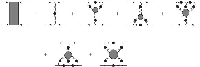
From Eq. (43 BDTR ; BCPQR 1 2
Figure 1: The gap equation up to the NNL-order truncation. The black circles indicate the propagators are fully dressed. The gray circles are connected Green’s functions. The dots are bare vertices.Figure 2: The meson BS kernel up to the NNL-order truncation. The gray rectangle is the BS kernel. The black circles indicate the propagators are fully dressed. The gray circles are connected Green’s functions. The dots are bare vertices.
As indicated in Introduction, RL truncation gives poor results in some channels, such as the scalar and axial-vector channels. The truncation scheme presented here allows us to make improvements in these channels. A few works have studied the impacts of going beyond the RL truncation by taking into account the three-gluon self-interaction FW ; WF ; AW ; FUW FW ; WF ; AW
Our framework automatically provide symmetry preserving truncations. The reason can be understood if we write the meson BSE in another form.
Actually, Eq. (42 Γ [ Φ ¯ , Π ¯ ] Γ ¯ Φ ¯ Π \Gamma[\bar{\Phi},\bar{\Pi}]
{ Φ ¯ − 1 , ρ 2 σ ′ δ 2 Γ δ Π ¯ σ ′ ρ ′ δ Φ ¯ σ 1 ρ 1 Φ ¯ − 1 , ρ ′ σ 2 + i δ 2 Γ δ Φ ¯ σ 2 ρ 2 δ Φ ¯ σ 1 ρ 1 } | Φ ¯ = Φ c , Π ¯ = Π c χ P , s ρ 2 σ 2 evaluated-at superscript ¯ Φ 1 subscript 𝜌 2 superscript 𝜎 ′
superscript 𝛿 2 Γ 𝛿 superscript ¯ Π superscript 𝜎 ′ superscript 𝜌 ′ 𝛿 superscript ¯ Φ subscript 𝜎 1 subscript 𝜌 1 superscript ¯ Φ 1 superscript 𝜌 ′ subscript 𝜎 2
𝑖 superscript 𝛿 2 Γ 𝛿 superscript ¯ Φ subscript 𝜎 2 subscript 𝜌 2 𝛿 superscript ¯ Φ subscript 𝜎 1 subscript 𝜌 1 formulae-sequence ¯ Φ subscript Φ 𝑐 ¯ Π subscript Π 𝑐 subscript superscript 𝜒 subscript 𝜌 2 subscript 𝜎 2 𝑃 𝑠
\displaystyle\left\{\bar{\Phi}^{-1,\rho_{2}\sigma^{\prime}}\frac{\delta^{2}\Gamma}{\delta\bar{\Pi}^{\sigma^{\prime}\rho^{\prime}}\delta\bar{\Phi}^{\sigma_{1}\rho_{1}}}\bar{\Phi}^{-1,\rho^{\prime}\sigma_{2}}+i\frac{\delta^{2}\Gamma}{\delta\bar{\Phi}^{\sigma_{2}\rho_{2}}\delta\bar{\Phi}^{\sigma_{1}\rho_{1}}}\right\}\bigg{|}_{\bar{\Phi}=\Phi_{c},\bar{\Pi}=\Pi_{c}}\chi^{\rho_{2}\sigma_{2}}_{P,s} = \displaystyle= 0 , 0 \displaystyle 0, (44)
where Γ [ Φ ¯ , Π ¯ ] Γ ¯ Φ ¯ Π \Gamma[\bar{\Phi},\bar{\Pi}] − i N c ln Z ′ | e . s . v . evaluated-at 𝑖 subscript 𝑁 𝑐 superscript 𝑍 ′ formulae-sequence e s v
\frac{-i}{N_{c}}\ln Z^{\prime}|_{\mathrm{e.s.v.}} Φ c , Π c subscript Φ 𝑐 subscript Π 𝑐
\Phi_{c},\Pi_{c} Φ ¯ , Π ¯ ¯ Φ ¯ Π
\bar{\Phi},\bar{\Pi}
Γ [ Φ ¯ , Π ¯ ] Γ ¯ Φ ¯ Π \displaystyle\Gamma[\bar{\Phi},\bar{\Pi}] = \displaystyle= − i Tr ln [ i ∂ / − M − Π ¯ ] + Φ ¯ σ ρ Π ¯ σ ρ + ∑ n = 2 ∞ ( − i ) n ( N c g 2 ) n − 1 n ! G ¯ ρ 1 ⋯ ρ n σ 1 ⋯ σ n Φ ¯ σ 1 ρ 1 ⋯ Φ ¯ σ n ρ n . \displaystyle-i{\rm Tr}\ln[i\partial\!\!\!/-M-\bar{\Pi}]+\bar{\Phi}^{\sigma\rho}\bar{\Pi}^{\sigma\rho}+\sum^{\infty}_{n=2}\frac{(-i)^{n}(N_{c}g^{2})^{n-1}}{n!}\bar{G}^{\sigma_{1}\cdots\sigma_{n}}_{\rho_{1}\cdots\rho_{n}}\bar{\Phi}^{\sigma_{1}\rho_{1}}\cdots\bar{\Phi}^{\sigma_{n}\rho_{n}}. (45)
Equation (44 Munczek − i ln Z ′ 𝑖 superscript 𝑍 ′ -i\ln Z^{\prime}
For the phenomenological studies focusing on meson properties under RL truncation, the gluon propagator is usually treated as an input, i.e. given as a model or by fitting lattice results, etc.. It avoids complications in dealing with too many coupled equations, thus is very useful for practical use. In our approach, the gauge sector and fermion sector of QCD are treated differently at the very beginning, so it retains the merit just mentioned. In this respect, our approach can be viewed as an extension from considering only the gluon propagator’s effects to considering higher-order gluon Green’s functions’ effects on the fermion sector. It results in truncations beyond the RL approximation on one hand and completes the gauge sector because of the inclusion of the gluon self-interactions on the other.
All the higher-order terms in our truncation scheme are originated from non-Abelian type dynamics, i.e., gluon self-interactions and gluon-ghost interactions. Remember that we have taken large N c subscript 𝑁 𝑐 N_{c}
V The Slavnov-Taylor identity for the quark-gluon vertex
The Slavnov-Taylor identity for the QGV provides an important constraint among the quark propagator, the QGV and the quark-ghost scattering kernel, which reflects the BRS symmetry of QCD. In principle, a proper truncation should guarantee solutions of truncated DSEs satisfy STIs. However it is not easy to maintain this requirement in practice. In order to see the explicit form of the STI of QGV in our formulism, we derive the quark-ghost scattering kernel in this section. Now, we need to express the Fadeev-Popov determinant in terms of ghost fields ϕ ¯ i ( x ) subscript ¯ italic-ϕ 𝑖 𝑥 \bar{\phi}_{i}(x) ϕ i ( x ) subscript italic-ϕ 𝑖 𝑥 \phi_{i}(x)
ℒ ghost = − ( ∂ μ ϕ ¯ i ) D i j μ ϕ j subscript ℒ ghost subscript 𝜇 superscript ¯ italic-ϕ 𝑖 subscript superscript 𝐷 𝜇 𝑖 𝑗 superscript italic-ϕ 𝑗 {\mathcal{L}}_{\mathrm{ghost}}=-(\partial_{\mu}\bar{\phi}^{i})D^{\mu}_{ij}\phi^{j} (46)
Using the BRS symmetry of the theory, one can arrive at a STI relating the quark-gluon 3-point Green’s function to the quark-antiquark-ghost-antighost 4-pont Green’s function PT
0 0 \displaystyle 0 = \displaystyle= ω { i 2 g λ α γ k ⟨ 0 | T [ ϕ k ( x ) ψ γ ( x ) ψ ¯ β ( y ) ϕ ¯ i ( z ) ] | 0 ⟩ f − i 2 g λ γ β k ⟨ 0 | T [ ψ α ( x ) ψ ¯ γ ( y ) ϕ k ( y ) ϕ ¯ i ( z ) ] | 0 ⟩ f \displaystyle\omega\bigg{\{}\frac{i}{2}g\lambda^{k}_{\alpha\gamma}\langle 0|T[\phi_{k}(x)\psi_{\gamma}(x)\bar{\psi}_{\beta}(y)\bar{\phi}_{i}(z)]|0\rangle_{f}-\frac{i}{2}g\lambda^{k}_{\gamma\beta}\langle 0|T[\psi_{\alpha}(x)\bar{\psi}_{\gamma}(y)\phi_{k}(y)\bar{\phi}_{i}(z)]|0\rangle_{f} (47)
+ 1 ξ ⟨ 0 | T [ ψ α ( x ) ψ ¯ β ( y ) ∂ μ A i μ ( z ) ] | 0 ⟩ f } . \displaystyle+\frac{1}{\xi}\langle 0|T[\psi_{\alpha}(x)\bar{\psi}_{\beta}(y)\partial_{\mu}A^{\mu}_{i}(z)]|0\rangle_{f}\bigg{\}}.
We shall see that this is just the STI for QGV.
Introducing the quark-ghost scattering kernels H α β i superscript subscript 𝐻 𝛼 𝛽 𝑖 H_{\alpha\beta}^{i} H ¯ α β i superscript subscript ¯ 𝐻 𝛼 𝛽 𝑖 \bar{H}_{\alpha\beta}^{i}
H α γ k ′ ( p , q , r ) S γ β ( r̸ ) D ~ k ′ i ( q 2 ) superscript subscript 𝐻 𝛼 𝛾 superscript 𝑘 ′ 𝑝 𝑞 𝑟 subscript 𝑆 𝛾 𝛽 italic-r̸ subscript ~ 𝐷 superscript 𝑘 ′ 𝑖 superscript 𝑞 2 \displaystyle H_{\alpha\gamma}^{k^{\prime}}(p,q,r)S_{\gamma\beta}(\not{r})\tilde{D}_{k^{\prime}i}(q^{2}) (48)
≡ \displaystyle\equiv 1 2 λ α γ k ∫ d 4 x d 4 y e − i p ⋅ x e − i r ⋅ y ⟨ 0 | T [ ϕ k ( x ) ψ γ ( x ) ψ ¯ β ( y ) ϕ ¯ i ( 0 ) ] | 0 ⟩ f 1 2 subscript superscript 𝜆 𝑘 𝛼 𝛾 superscript 𝑑 4 𝑥 superscript 𝑑 4 𝑦 superscript 𝑒 ⋅ 𝑖 𝑝 𝑥 superscript 𝑒 ⋅ 𝑖 𝑟 𝑦 subscript quantum-operator-product 0 𝑇 delimited-[] subscript italic-ϕ 𝑘 𝑥 subscript 𝜓 𝛾 𝑥 subscript ¯ 𝜓 𝛽 𝑦 subscript ¯ italic-ϕ 𝑖 0 0 𝑓 \displaystyle\frac{1}{2}\lambda^{k}_{\alpha\gamma}\int d^{4}xd^{4}ye^{-ip\cdot x}e^{-ir\cdot y}\langle 0|T[\phi_{k}(x)\psi_{\gamma}(x)\bar{\psi}_{\beta}(y)\bar{\phi}_{i}(0)]|0\rangle_{f}
and
S α γ ( − p̸ ) H ¯ γ β k ′ ( − r , − q , − p ) D ~ k ′ i ( q 2 ) subscript 𝑆 𝛼 𝛾 italic-p̸ superscript subscript ¯ 𝐻 𝛾 𝛽 superscript 𝑘 ′ 𝑟 𝑞 𝑝 subscript ~ 𝐷 superscript 𝑘 ′ 𝑖 superscript 𝑞 2 \displaystyle S_{\alpha\gamma}(-\not{p})\bar{H}_{\gamma\beta}^{k^{\prime}}(-r,-q,-p)\tilde{D}_{k^{\prime}i}(q^{2}) (49)
≡ \displaystyle\equiv 1 2 λ γ β k ∫ d 4 x d 4 y e − i p ⋅ x e − i r ⋅ y ⟨ 0 | T [ ψ α ( x ) ψ ¯ γ ( y ) ϕ k ( y ) ϕ ¯ i ( 0 ) ] | 0 ⟩ f 1 2 subscript superscript 𝜆 𝑘 𝛾 𝛽 superscript 𝑑 4 𝑥 superscript 𝑑 4 𝑦 superscript 𝑒 ⋅ 𝑖 𝑝 𝑥 superscript 𝑒 ⋅ 𝑖 𝑟 𝑦 subscript quantum-operator-product 0 𝑇 delimited-[] subscript 𝜓 𝛼 𝑥 subscript ¯ 𝜓 𝛾 𝑦 subscript italic-ϕ 𝑘 𝑦 subscript ¯ italic-ϕ 𝑖 0 0 𝑓 \displaystyle\frac{1}{2}\lambda^{k}_{\gamma\beta}\int d^{4}xd^{4}ye^{-ip\cdot x}e^{-ir\cdot y}\langle 0|T[\psi_{\alpha}(x)\bar{\psi}_{\gamma}(y)\phi_{k}(y)\bar{\phi}_{i}(0)]|0\rangle_{f}
where q = − p − r 𝑞 𝑝 𝑟 q=-p-r D ~ i j ( q 2 ) subscript ~ 𝐷 𝑖 𝑗 superscript 𝑞 2 \tilde{D}_{ij}(q^{2}) 47
g H α γ k ′ ( p , q , r ) S γ β ( r̸ ) D ~ k ′ i ( q 2 ) − g S α γ ( − p̸ ) H ¯ γ β k ′ ( − r , − q , − p ) D ~ k ′ i ( q 2 ) 𝑔 superscript subscript 𝐻 𝛼 𝛾 superscript 𝑘 ′ 𝑝 𝑞 𝑟 subscript 𝑆 𝛾 𝛽 italic-r̸ subscript ~ 𝐷 superscript 𝑘 ′ 𝑖 superscript 𝑞 2 𝑔 subscript 𝑆 𝛼 𝛾 italic-p̸ superscript subscript ¯ 𝐻 𝛾 𝛽 superscript 𝑘 ′ 𝑟 𝑞 𝑝 subscript ~ 𝐷 superscript 𝑘 ′ 𝑖 superscript 𝑞 2 \displaystyle gH_{\alpha\gamma}^{k^{\prime}}(p,q,r)S_{\gamma\beta}(\not{r})\tilde{D}_{k^{\prime}i}(q^{2})-gS_{\alpha\gamma}(-\not{p})\bar{H}_{\gamma\beta}^{k^{\prime}}(-r,-q,-p)\tilde{D}_{k^{\prime}i}(q^{2}) (50)
= \displaystyle= 1 ξ S α γ ( − p̸ ) [ − i g Γ ν , γ α j ( q , p , r ) ] S α β ( r̸ ) G j i ν μ ( q ) q μ . 1 𝜉 subscript 𝑆 𝛼 𝛾 italic-p̸ delimited-[] 𝑖 𝑔 superscript subscript Γ 𝜈 𝛾 𝛼
𝑗 𝑞 𝑝 𝑟 subscript 𝑆 𝛼 𝛽 italic-r̸ subscript superscript 𝐺 𝜈 𝜇 𝑗 𝑖 𝑞 subscript 𝑞 𝜇 \displaystyle\frac{1}{\xi}S_{\alpha\gamma}(-\not{p})\big{[}-ig\Gamma_{\nu,\gamma\alpha}^{j}(q,p,r)\big{]}S_{\alpha\beta}(\not{r})G^{\nu\mu}_{ji}(q)q_{\mu}.
Since for the gluon propagator G j i ν μ ( q ) subscript superscript 𝐺 𝜈 𝜇 𝑗 𝑖 𝑞 G^{\nu\mu}_{ji}(q)
S − 1 ( − p̸ ) H ( p , q , r ) − H ¯ ( − r , − q , − p ) S − 1 ( − r̸ ) superscript 𝑆 1 italic-p̸ 𝐻 𝑝 𝑞 𝑟 ¯ 𝐻 𝑟 𝑞 𝑝 superscript 𝑆 1 italic-r̸ \displaystyle S^{-1}(-\not{p})H(p,q,r)-\bar{H}(-r,-q,-p)S^{-1}(-\not{r}) = \displaystyle= − 1 q 2 q ν Γ ν ( q , p , r ) D ~ − 1 ( q 2 ) , 1 superscript 𝑞 2 superscript 𝑞 𝜈 subscript Γ 𝜈 𝑞 𝑝 𝑟 superscript ~ 𝐷 1 superscript 𝑞 2 \displaystyle-\frac{1}{q^{2}}q^{\nu}\Gamma_{\nu}(q,p,r)\tilde{D}^{-1}(q^{2}), (51)
which is just the usual form of the STI of QGV.
In QED, ghost fields decouple from other fields, i.e., H = H ¯ = 1 𝐻 ¯ 𝐻 1 H=\bar{H}=1 D ~ − 1 ( q 2 ) = − q 2 superscript ~ 𝐷 1 superscript 𝑞 2 superscript 𝑞 2 \tilde{D}^{-1}(q^{2})=-q^{2}
S − 1 ( − p̸ ) − S − 1 ( − r̸ ) superscript 𝑆 1 italic-p̸ superscript 𝑆 1 italic-r̸ \displaystyle S^{-1}(-\not{p})-S^{-1}(-\not{r}) = \displaystyle= q ν Γ ν ( q , p , r ) superscript 𝑞 𝜈 subscript Γ 𝜈 𝑞 𝑝 𝑟 \displaystyle q^{\nu}\Gamma_{\nu}(q,p,r) (52)
Without taking large N c subscript 𝑁 𝑐 N_{c} S U ( N c ) 𝑆 𝑈 subscript 𝑁 𝑐 SU(N_{c}) N c subscript 𝑁 𝑐 N_{c} N c subscript 𝑁 𝑐 N_{c} 51 η ¯ η ¯ 𝜂 𝜂 \bar{\eta}\eta N c subscript 𝑁 𝑐 N_{c} 86
Now the quark-antiquark-ghost-antighost 4-pont Green’s function can be derived directly by calculating − i δ 4 ln Z ′ δ η ¯ j δ ( − η i ) δ I ¯ β δ ( − I α ) 𝑖 superscript 𝛿 4 superscript 𝑍 ′ 𝛿 superscript ¯ 𝜂 𝑗 𝛿 superscript 𝜂 𝑖 𝛿 subscript ¯ 𝐼 𝛽 𝛿 subscript 𝐼 𝛼 \frac{-i\delta^{4}\ln Z^{\prime}}{\delta\bar{\eta}^{j}\delta(-\eta^{i})\delta\bar{I}_{\beta}\delta(-I_{\alpha})}
⟨ 0 | T [ ϕ j ( y ~ ) ϕ ¯ i ( x ~ ) ψ β ρ ( y ) ψ ¯ α σ ( x ) ] | 0 ⟩ c subscript quantum-operator-product 0 𝑇 delimited-[] subscript italic-ϕ 𝑗 ~ 𝑦 subscript ¯ italic-ϕ 𝑖 ~ 𝑥 superscript subscript 𝜓 𝛽 𝜌 𝑦 superscript subscript ¯ 𝜓 𝛼 𝜎 𝑥 0 𝑐 \displaystyle\langle 0|T[\phi_{j}(\tilde{y})\bar{\phi}_{i}(\tilde{x})\psi_{\beta}^{\rho}(y)\bar{\psi}_{\alpha}^{\sigma}(x)]|0\rangle_{c}
= \displaystyle= ∫ d 4 x ′ d 4 y ′ [ − ( i ∂ / − M − Π c ) ρ ρ ′ − 1 ( y , y ′ ) δ 2 Π c ρ ′ σ ′ ( y ′ , x ′ ) δ η ¯ j ( y ~ ) δ ( − η i ( x ~ ) ) ( i ∂ / − M − Π c ) σ ′ σ − 1 ( x ′ , x ) ] δ α β \displaystyle\int d^{4}x^{\prime}d^{4}y^{\prime}\bigg{[}-(i\partial\!\!\!/-M-\Pi_{c})^{-1}_{\rho\rho^{\prime}}(y,y^{\prime})\frac{\delta^{2}\Pi_{c}^{\rho^{\prime}\sigma^{\prime}}(y^{\prime},x^{\prime})}{\delta\bar{\eta}^{j}(\tilde{y})\delta(-\eta^{i}(\tilde{x}))}(i\partial\!\!\!/-M-\Pi_{c})^{-1}_{\sigma^{\prime}\sigma}(x^{\prime},x)\bigg{]}\delta_{\alpha\beta}
+ ∫ d 4 x ′ d 4 y ′ [ ( i ∂ / − M − Π c ) ρ ρ ′ − 1 ( y , y ′ ) ( Δ Φ c b ρ ′ σ ′ ( x ~ , y ~ ; y ′ , x ′ ) [ λ i λ j ] β α \displaystyle+\int d^{4}x^{\prime}d^{4}y^{\prime}\bigg{[}(i\partial\!\!\!/-M-\Pi_{c})^{-1}_{\rho\rho^{\prime}}(y,y^{\prime})\big{(}\Delta^{b\rho^{\prime}\sigma^{\prime}}_{\Phi_{c}}(\tilde{x},\tilde{y};y^{\prime},x^{\prime})[\lambda^{i}\lambda^{j}]_{\beta\alpha}
+ Δ Φ c c ρ ′ σ ′ ( x ~ , y ~ ; y ′ , x ′ ) [ λ j λ i ] β α ) ( i ∂ / − M − Π c ) σ ′ σ − 1 ( x ′ , x ) ] . \displaystyle\hskip 56.9055pt+\Delta^{c\rho^{\prime}\sigma^{\prime}}_{\Phi_{c}}(\tilde{x},\tilde{y};y^{\prime},x^{\prime})[\lambda^{j}\lambda^{i}]_{\beta\alpha}\big{)}(i\partial\!\!\!/-M-\Pi_{c})^{-1}_{\sigma^{\prime}\sigma}(x^{\prime},x)\bigg{]}.
The full Green’s function is
⟨ 0 | T [ ϕ j ( y ~ ) ϕ ¯ i ( x ~ ) ψ β ρ ( y ) ψ ¯ α σ ( x ) ] | 0 ⟩ f subscript quantum-operator-product 0 𝑇 delimited-[] subscript italic-ϕ 𝑗 ~ 𝑦 subscript ¯ italic-ϕ 𝑖 ~ 𝑥 superscript subscript 𝜓 𝛽 𝜌 𝑦 superscript subscript ¯ 𝜓 𝛼 𝜎 𝑥 0 𝑓 \displaystyle\langle 0|T[\phi_{j}(\tilde{y})\bar{\phi}_{i}(\tilde{x})\psi_{\beta}^{\rho}(y)\bar{\psi}_{\alpha}^{\sigma}(x)]|0\rangle_{f} (54)
= \displaystyle= i ⟨ 0 | T [ ϕ j ( y ~ ) ϕ ¯ i ( x ~ ) ψ β ρ ( y ) ψ ¯ α σ ( x ) ] | 0 ⟩ c − ⟨ 0 | T [ ψ β ρ ( y ) ψ ¯ α σ ( x ) ] | 0 ⟩ c ⟨ 0 | T [ ϕ j ( y ~ ) ϕ ¯ i ( x ~ ) ] | 0 ⟩ c 𝑖 subscript quantum-operator-product 0 𝑇 delimited-[] subscript italic-ϕ 𝑗 ~ 𝑦 subscript ¯ italic-ϕ 𝑖 ~ 𝑥 superscript subscript 𝜓 𝛽 𝜌 𝑦 superscript subscript ¯ 𝜓 𝛼 𝜎 𝑥 0 𝑐 subscript quantum-operator-product 0 𝑇 delimited-[] superscript subscript 𝜓 𝛽 𝜌 𝑦 superscript subscript ¯ 𝜓 𝛼 𝜎 𝑥 0 𝑐 subscript quantum-operator-product 0 𝑇 delimited-[] subscript italic-ϕ 𝑗 ~ 𝑦 subscript ¯ italic-ϕ 𝑖 ~ 𝑥 0 𝑐 \displaystyle i\langle 0|T[\phi_{j}(\tilde{y})\bar{\phi}_{i}(\tilde{x})\psi_{\beta}^{\rho}(y)\bar{\psi}_{\alpha}^{\sigma}(x)]|0\rangle_{c}-\langle 0|T[\psi_{\beta}^{\rho}(y)\bar{\psi}_{\alpha}^{\sigma}(x)]|0\rangle_{c}\langle 0|T[\phi_{j}(\tilde{y})\bar{\phi}_{i}(\tilde{x})]|0\rangle_{c}
= \displaystyle= ∫ d 4 x ′ d 4 y ′ [ − ( i ∂ / − M − Π c ) ρ ρ ′ − 1 ( y , y ′ ) i δ 2 Π c ρ ′ σ ′ ( y ′ , x ′ ) δ η ¯ j ( y ~ ) δ ( − η i ( x ~ ) ) ( i ∂ / − M − Π c ) σ ′ σ − 1 ( x ′ , x ) ] δ α β \displaystyle\int d^{4}x^{\prime}d^{4}y^{\prime}\bigg{[}-(i\partial\!\!\!/-M-\Pi_{c})^{-1}_{\rho\rho^{\prime}}(y,y^{\prime})\frac{i\delta^{2}\Pi_{c}^{\rho^{\prime}\sigma^{\prime}}(y^{\prime},x^{\prime})}{\delta\bar{\eta}^{j}(\tilde{y})\delta(-\eta^{i}(\tilde{x}))}(i\partial\!\!\!/-M-\Pi_{c})^{-1}_{\sigma^{\prime}\sigma}(x^{\prime},x)\bigg{]}\delta_{\alpha\beta}
+ ∫ d 4 x ′ d 4 y ′ [ ( i ∂ / − M − Π c ) ρ ρ ′ − 1 ( y , y ′ ) ( i Δ Φ c b ρ ′ σ ′ ( x ~ , y ~ ; y ′ , x ′ ) [ λ i λ j ] β α \displaystyle+\int d^{4}x^{\prime}d^{4}y^{\prime}\bigg{[}(i\partial\!\!\!/-M-\Pi_{c})^{-1}_{\rho\rho^{\prime}}(y,y^{\prime})\big{(}i\Delta^{b\rho^{\prime}\sigma^{\prime}}_{\Phi_{c}}(\tilde{x},\tilde{y};y^{\prime},x^{\prime})[\lambda^{i}\lambda^{j}]_{\beta\alpha}
+ i Δ Φ c c ρ ′ σ ′ ( x ~ , y ~ ; y ′ , x ′ ) [ λ j λ i ] β α ) ( i ∂ / − M − Π c ) σ ′ σ − 1 ( x ′ , x ) ] \displaystyle\hskip 56.9055pt+i\Delta^{c\rho^{\prime}\sigma^{\prime}}_{\Phi_{c}}(\tilde{x},\tilde{y};y^{\prime},x^{\prime})[\lambda^{j}\lambda^{i}]_{\beta\alpha}\big{)}(i\partial\!\!\!/-M-\Pi_{c})^{-1}_{\sigma^{\prime}\sigma}(x^{\prime},x)\bigg{]}
− δ α β δ i j ( i ∂ / − M − Π c ) ρ σ − 1 ( y , x ) D ~ ( x ~ , y ~ ) . \displaystyle-\delta_{\alpha\beta}\delta_{ij}(i\partial\!\!\!/-M-\Pi_{c})^{-1}_{\rho\sigma}(y,x)\tilde{D}(\tilde{x},\tilde{y}).
Taking Eq. (24 54 47
λ α β i ( i g 2 ) ∫ d 4 x ′ d 4 y ′ ( i ∂ / − M − Π c ) ρ ρ ′ − 1 ( x , y ′ ) { − i δ 2 Π c ρ ′ σ ′ ( y ′ , x ′ ) δ η ¯ j ( x ) δ ( − η i ( z ) ) + i δ 2 Π c ρ ′ σ ′ ( y ′ , x ′ ) δ η ¯ j ( y ) δ ( − η i ( z ) ) \displaystyle\lambda^{i}_{\alpha\beta}(\frac{ig}{2})\int d^{4}x^{\prime}d^{4}y^{\prime}(i\partial\!\!\!/-M-\Pi_{c})^{-1}_{\rho\rho^{\prime}}(x,y^{\prime})\bigg{\{}-\frac{i\delta^{2}\Pi_{c}^{\rho^{\prime}\sigma^{\prime}}(y^{\prime},x^{\prime})}{\delta\bar{\eta}^{j}(x)\delta(-\eta^{i}(z))}+\frac{i\delta^{2}\Pi_{c}^{\rho^{\prime}\sigma^{\prime}}(y^{\prime},x^{\prime})}{\delta\bar{\eta}^{j}(y)\delta(-\eta^{i}(z))} (55)
+ 2 N c ( i Δ Φ c c ρ ′ σ ′ ( z , x ; y ′ , x ′ ) − i Δ Φ c b ρ ′ σ ′ ( z , y ; y ′ , x ′ ) ) 2 subscript 𝑁 𝑐 𝑖 subscript superscript Δ 𝑐 superscript 𝜌 ′ superscript 𝜎 ′ subscript Φ 𝑐 𝑧 𝑥 superscript 𝑦 ′ superscript 𝑥 ′ 𝑖 subscript superscript Δ 𝑏 superscript 𝜌 ′ superscript 𝜎 ′ subscript Φ 𝑐 𝑧 𝑦 superscript 𝑦 ′ superscript 𝑥 ′ \displaystyle\hskip 170.71652pt+2N_{c}\big{(}i\Delta^{c\rho^{\prime}\sigma^{\prime}}_{\Phi_{c}}(z,x;y^{\prime},x^{\prime})-i\Delta^{b\rho^{\prime}\sigma^{\prime}}_{\Phi_{c}}(z,y;y^{\prime},x^{\prime})\big{)}
+ ( i ∂ / − M − Π c ) ρ ′ σ ′ ( y ′ , x ′ ) ( D ~ ( z , x ) − D ~ ( z , y ) ) } ( i ∂ / − M − Π c ) − 1 σ ′ σ ( x ′ , y ) \displaystyle\hskip 170.71652pt+(i\partial\!\!\!/-M-\Pi_{c})_{\rho^{\prime}\sigma^{\prime}}(y^{\prime},x^{\prime})\big{(}\tilde{D}(z,x)-\tilde{D}(z,y)\big{)}\bigg{\}}(i\partial\!\!\!/-M-\Pi_{c})^{-1}_{\sigma^{\prime}\sigma}(x^{\prime},y)
= \displaystyle= λ α β i ∫ d 4 x ′ d 4 y ′ ( i ∂ / − M − Π c ) ρ ρ ′ − 1 ( x , y ′ ) [ − 1 ξ ∂ ∂ z μ Δ Φ c μ ρ ′ σ ′ ( z , y ′ , x ′ ) ] ( i ∂ / − M − Π c ) σ ′ σ − 1 ( x ′ , y ) . \displaystyle\lambda^{i}_{\alpha\beta}\int d^{4}x^{\prime}d^{4}y^{\prime}(i\partial\!\!\!/-M-\Pi_{c})^{-1}_{\rho\rho^{\prime}}(x,y^{\prime})\bigg{[}-\frac{1}{\xi}\frac{\partial}{\partial z^{\mu}}\Delta_{\Phi_{c}}^{\mu\rho^{\prime}\sigma^{\prime}}(z,y^{\prime},x^{\prime})\bigg{]}(i\partial\!\!\!/-M-\Pi_{c})^{-1}_{\sigma^{\prime}\sigma}(x^{\prime},y).
This is the STI for QGV in our formalism.
The undetermined function δ 2 Π c ρ ′ σ ′ ( y ′ , x ′ ) δ η ¯ j ( x ) δ ( − η i ( z ) ) superscript 𝛿 2 superscript subscript Π 𝑐 superscript 𝜌 ′ superscript 𝜎 ′ superscript 𝑦 ′ superscript 𝑥 ′ 𝛿 superscript ¯ 𝜂 𝑗 𝑥 𝛿 superscript 𝜂 𝑖 𝑧 \frac{\delta^{2}\Pi_{c}^{\rho^{\prime}\sigma^{\prime}}(y^{\prime},x^{\prime})}{\delta\bar{\eta}^{j}(x)\delta(-\eta^{i}(z))}
δ 2 Π c δ η ¯ j δ ( − η i ) superscript 𝛿 2 subscript Π 𝑐 𝛿 superscript ¯ 𝜂 𝑗 𝛿 superscript 𝜂 𝑖 \displaystyle\frac{\delta^{2}\Pi_{c}}{\delta\bar{\eta}^{j}\delta(-\eta^{i})} = \displaystyle= i δ i j 2 N c Tr [ ( i ∂ / − M − Π c ) − 1 ( δ Δ Φ c b δ Φ c + δ Δ Φ c c δ Φ c ) ] \displaystyle i\frac{\delta_{ij}}{2N_{c}}\mathrm{Tr}\big{[}(i\partial\!\!\!/-M-\Pi_{c})^{-1}\big{(}\frac{\delta\Delta^{b}_{\Phi_{c}}}{\delta\Phi_{c}}+\frac{\delta\Delta^{c}_{\Phi_{c}}}{\delta\Phi_{c}}\big{)}\big{]} (56)
− δ i j N c δ Δ Φ c a δ Φ c − δ Δ Φ c d N c δ Φ c ⟨ ψ ¯ λ i ψ ⟩ ⟨ ψ ¯ λ j ψ ⟩ subscript 𝛿 𝑖 𝑗 subscript 𝑁 𝑐 𝛿 subscript superscript Δ 𝑎 subscript Φ 𝑐 𝛿 subscript Φ 𝑐 𝛿 subscript superscript Δ 𝑑 subscript Φ 𝑐 subscript 𝑁 𝑐 𝛿 subscript Φ 𝑐 delimited-⟨⟩ ¯ 𝜓 superscript 𝜆 𝑖 𝜓 delimited-⟨⟩ ¯ 𝜓 superscript 𝜆 𝑗 𝜓 \displaystyle-\frac{\delta_{ij}}{N_{c}}\frac{\delta\Delta^{a}_{\Phi_{c}}}{\delta\Phi_{c}}-\frac{\delta\Delta^{d}_{\Phi_{c}}}{N_{c}\delta\Phi_{c}}\langle\bar{\psi}\lambda^{i}\psi\rangle\langle\bar{\psi}\lambda^{j}\psi\rangle
+ ∑ n = 2 ∞ ( − i ) n ( N c g 2 ) n − 1 ( n − 2 ) ! G ¯ n − 1 δ 2 Φ c δ η ¯ j δ ( − η i ) Φ c ⋯ Φ c , subscript superscript 𝑛 2 superscript 𝑖 𝑛 superscript subscript 𝑁 𝑐 superscript 𝑔 2 𝑛 1 𝑛 2 subscript ¯ 𝐺 𝑛 1 superscript 𝛿 2 subscript Φ 𝑐 𝛿 superscript ¯ 𝜂 𝑗 𝛿 superscript 𝜂 𝑖 subscript Φ 𝑐 ⋯ subscript Φ 𝑐 \displaystyle+\sum^{\infty}_{n=2}\frac{(-i)^{n}(N_{c}g^{2})^{n-1}}{(n-2)!}\bar{G}_{n-1}\frac{\delta^{2}\Phi_{c}}{\delta\bar{\eta}^{j}\delta(-\eta^{i})}\Phi_{c}\cdots\Phi_{c},
δ 2 Φ c δ η ¯ j δ ( − η i ) superscript 𝛿 2 subscript Φ 𝑐 𝛿 superscript ¯ 𝜂 𝑗 𝛿 superscript 𝜂 𝑖 \displaystyle\frac{\delta^{2}\Phi_{c}}{\delta\bar{\eta}^{j}\delta(-\eta^{i})} = \displaystyle= − i ( i ∂ / − M − Π c ) − 1 δ 2 Π c δ η ¯ j δ ( − η i ) ( i ∂ / − M − Π c ) − 1 \displaystyle-i(i\partial\!\!\!/-M-\Pi_{c})^{-1}\frac{\delta^{2}\Pi_{c}}{\delta\bar{\eta}^{j}\delta(-\eta^{i})}(i\partial\!\!\!/-M-\Pi_{c})^{-1} (57)
+ i δ i j 2 N c Tr [ ( i ∂ / − M − Π c ) − 1 ( Δ Φ c b + Δ Φ c c ) ] . \displaystyle+i\frac{\delta_{ij}}{2N_{c}}\mathrm{Tr}\big{[}(i\partial\!\!\!/-M-\Pi_{c})^{-1}\big{(}\Delta^{b}_{\Phi_{c}}+\Delta^{c}_{\Phi_{c}}\big{)}\big{]}.
Δ Φ c a , Δ Φ c b , Δ Φ c c superscript subscript Δ subscript Φ 𝑐 𝑎 superscript subscript Δ subscript Φ 𝑐 𝑏 superscript subscript Δ subscript Φ 𝑐 𝑐
\Delta_{\Phi_{c}}^{a},\Delta_{\Phi_{c}}^{b},\Delta_{\Phi_{c}}^{c} Δ Φ c d superscript subscript Δ subscript Φ 𝑐 𝑑 \Delta_{\Phi_{c}}^{d} 55 Δ Φ c μ superscript subscript Δ subscript Φ 𝑐 𝜇 \Delta_{\Phi_{c}}^{\mu} 55
We have given the expression of the quark-antiquark-ghost-antighost 4-pont Green’s function (Eq. (54 55 N c subscript 𝑁 𝑐 N_{c} 55 55
VI Summary
We introduced an alternate form for the QCD generating functional which is a generalization of the one used in a previous study. This form has the power to address various nonperturbative problems in QCD. Specifically, we employed it to study Dyson-Schwinger Equations and Bethe-Salpeter Equation and their truncations. The large N c subscript 𝑁 𝑐 N_{c} N c subscript 𝑁 𝑐 N_{c} N c subscript 𝑁 𝑐 N_{c}
Since the explicit forms of the DSEs and the BSE are established at large N c subscript 𝑁 𝑐 N_{c} 1 / N c 1 subscript 𝑁 𝑐 1/N_{c} N c subscript 𝑁 𝑐 N_{c}
In order to study the QGV STI, we derived the quark-ghost scattering kernel. Ghost fields are explicitly shown in the generating functional and the external sources are introduced. Although we cannot verify the STI directly due to the complicated form of the quark-ghost scattering kernel, we hope those discussions could shed some light on further studies and on the modeling of QGV using the STI.
Appendix A
In this appendix, we give a detailed discussion on the Fierz reordering. In order to obtain Eq. (7
G μ 1 μ 2 i 1 i 2 ( x 1 , x 2 ) [ − g ψ ¯ α 1 a 1 ( x 1 ) ( λ i 1 2 ) α 1 β 1 γ μ 1 ψ β 1 a 1 ( x 1 ) ] [ − g ψ ¯ α 2 a 2 ( x 2 ) ( λ i 2 2 ) α 2 β 2 γ μ 2 ψ β 2 a 2 ( x 2 ) ] superscript subscript 𝐺 subscript 𝜇 1 subscript 𝜇 2 subscript 𝑖 1 subscript 𝑖 2 subscript 𝑥 1 subscript 𝑥 2 delimited-[] 𝑔 subscript superscript ¯ 𝜓 subscript 𝑎 1 subscript 𝛼 1 subscript 𝑥 1 subscript subscript 𝜆 subscript 𝑖 1 2 subscript 𝛼 1 subscript 𝛽 1 superscript 𝛾 subscript 𝜇 1 subscript superscript 𝜓 subscript 𝑎 1 subscript 𝛽 1 subscript 𝑥 1 delimited-[] 𝑔 subscript superscript ¯ 𝜓 subscript 𝑎 2 subscript 𝛼 2 subscript 𝑥 2 subscript subscript 𝜆 subscript 𝑖 2 2 subscript 𝛼 2 subscript 𝛽 2 superscript 𝛾 subscript 𝜇 2 subscript superscript 𝜓 subscript 𝑎 2 subscript 𝛽 2 subscript 𝑥 2 \displaystyle G_{\mu_{1}\mu_{2}}^{i_{1}i_{2}}(x_{1},x_{2})[-g\bar{\psi}^{a_{1}}_{{\alpha}_{1}}(x_{1})(\frac{\lambda_{i_{1}}}{2})_{\alpha_{1}\beta_{1}}\gamma^{\mu_{1}}{\psi}^{a_{1}}_{{\beta}_{1}}(x_{1})][-g\bar{\psi}^{a_{2}}_{{\alpha}_{2}}(x_{2})(\frac{\lambda_{i_{2}}}{2})_{\alpha_{2}\beta_{2}}\gamma^{\mu_{2}}{\psi}^{a_{2}}_{\beta_{2}}(x_{2})]
= G μ 1 μ 2 ( x 1 , x 2 ) [ − g ψ ¯ α 1 a 1 ( x 1 ) γ μ 1 ψ β 1 a 1 ( x 1 ) ] [ − g ψ ¯ α 2 a 2 ( x 2 ) γ μ 2 ψ β 2 a 2 ( x 2 ) ] 1 2 ( δ α 1 β 2 δ α 2 β 1 − 1 N c δ α 1 β 1 δ α 2 β 2 ) absent subscript 𝐺 subscript 𝜇 1 subscript 𝜇 2 subscript 𝑥 1 subscript 𝑥 2 delimited-[] 𝑔 subscript superscript ¯ 𝜓 subscript 𝑎 1 subscript 𝛼 1 subscript 𝑥 1 superscript 𝛾 subscript 𝜇 1 subscript superscript 𝜓 subscript 𝑎 1 subscript 𝛽 1 subscript 𝑥 1 delimited-[] 𝑔 subscript superscript ¯ 𝜓 subscript 𝑎 2 subscript 𝛼 2 subscript 𝑥 2 superscript 𝛾 subscript 𝜇 2 subscript superscript 𝜓 subscript 𝑎 2 subscript 𝛽 2 subscript 𝑥 2 1 2 subscript 𝛿 subscript 𝛼 1 subscript 𝛽 2 subscript 𝛿 subscript 𝛼 2 subscript 𝛽 1 1 subscript 𝑁 𝑐 subscript 𝛿 subscript 𝛼 1 subscript 𝛽 1 subscript 𝛿 subscript 𝛼 2 subscript 𝛽 2 \displaystyle=G_{\mu_{1}\mu_{2}}(x_{1},x_{2})[-g\bar{\psi}^{a_{1}}_{{\alpha}_{1}}(x_{1})\gamma^{\mu_{1}}{\psi}^{a_{1}}_{{\beta}_{1}}(x_{1})][-g\bar{\psi}^{a_{2}}_{{\alpha}_{2}}(x_{2})\gamma^{\mu_{2}}{\psi}^{a_{2}}_{\beta_{2}}(x_{2})]\frac{1}{2}(\delta_{\alpha_{1}\beta_{2}}\delta_{\alpha_{2}\beta_{1}}-\frac{1}{N_{c}}\delta_{\alpha_{1}\beta_{1}}\delta_{\alpha_{2}\beta_{2}})
= ∫ d 4 x 1 ′ d 4 x 2 ′ g 2 G μ 1 μ 2 ( x 1 , x 2 ) [ − 1 2 ( γ μ 1 ) σ 1 ρ 2 ( γ μ 2 ) σ 2 ρ 1 δ ( x 1 ′ − x 2 ) δ ( x 2 ′ − x 1 ) \displaystyle=\int d^{4}x_{1}^{\prime}d^{4}x_{2}^{\prime}~{}g^{2}G_{\mu_{1}\mu_{2}}(x_{1},x_{2})[-\frac{1}{2}(\gamma^{\mu_{1}})_{\sigma_{1}\rho_{2}}(\gamma^{\mu_{2}})_{\sigma_{2}\rho_{1}}\delta(x_{1}^{\prime}-x_{2})\delta(x_{2}^{\prime}-x_{1})
− 1 2 N c ( γ μ 1 ) σ 1 ρ 1 ( γ μ 2 ) σ 2 ρ 2 δ ( x 1 ′ − x 1 ) δ ( x 2 ′ − x 2 ) ] ψ ¯ α 1 σ 1 ( x 1 ) ψ α 1 ρ 1 ( x 1 ′ ) ψ ¯ α 2 σ 2 ( x 2 ) ψ α 2 ρ 2 ( x 2 ′ ) . \displaystyle\hskip 14.22636pt-\frac{1}{2N_{c}}(\gamma^{\mu_{1}})_{\sigma_{1}\rho_{1}}(\gamma^{\mu_{2}})_{\sigma_{2}\rho_{2}}\delta(x_{1}^{\prime}-x_{1})\delta(x_{2}^{\prime}-x_{2})]\bar{\psi}_{\alpha_{1}}^{\sigma_{1}}(x_{1})\psi_{\alpha_{1}}^{\rho_{1}}(x_{1}^{\prime})\bar{\psi}_{\alpha_{2}}^{\sigma_{2}}(x_{2})\psi_{\alpha_{2}}^{\rho_{2}}(x_{2}^{\prime}). (58)
In obtaining the above result, we have used relations
G μ 1 μ 2 i 1 i 2 ( x 1 , x 2 ) = δ i 1 i 2 G μ 1 μ 2 ( x 1 , x 2 ) , superscript subscript 𝐺 subscript 𝜇 1 subscript 𝜇 2 subscript 𝑖 1 subscript 𝑖 2 subscript 𝑥 1 subscript 𝑥 2 superscript 𝛿 subscript 𝑖 1 subscript 𝑖 2 subscript 𝐺 subscript 𝜇 1 subscript 𝜇 2 subscript 𝑥 1 subscript 𝑥 2 \displaystyle G_{\mu_{1}\mu_{2}}^{i_{1}i_{2}}(x_{1},x_{2})=\delta^{i_{1}i_{2}}G_{\mu_{1}\mu_{2}}(x_{1},x_{2}), (59)
( λ i 2 ) α 1 β 1 ( λ i 2 ) α 2 β 2 = 1 2 ( δ α 1 β 2 δ α 2 β 1 − 1 N c δ α 1 β 1 δ α 2 β 2 ) . subscript subscript 𝜆 𝑖 2 subscript 𝛼 1 subscript 𝛽 1 subscript subscript 𝜆 𝑖 2 subscript 𝛼 2 subscript 𝛽 2 1 2 subscript 𝛿 subscript 𝛼 1 subscript 𝛽 2 subscript 𝛿 subscript 𝛼 2 subscript 𝛽 1 1 subscript 𝑁 𝑐 subscript 𝛿 subscript 𝛼 1 subscript 𝛽 1 subscript 𝛿 subscript 𝛼 2 subscript 𝛽 2 \displaystyle(\frac{\lambda_{i}}{2})_{\alpha_{1}\beta_{1}}(\frac{\lambda_{i}}{2})_{\alpha_{2}\beta_{2}}=\frac{1}{2}(\delta_{\alpha_{1}\beta_{2}}\delta_{\alpha_{2}\beta_{1}}-\frac{1}{N_{c}}\delta_{\alpha_{1}\beta_{1}}\delta_{\alpha_{2}\beta_{2}}). (60)
Hence the extended 2-point Green’s function is
G ¯ ρ 1 ρ 2 σ 1 σ 2 ( x 1 , x 1 ′ , x 2 , x 2 ′ ) = − 1 2 G μ 1 μ 2 ( x 1 , x 2 ) [ \displaystyle\overline{G}_{\rho_{1}\rho_{2}}^{\sigma_{1}\sigma_{2}}(x_{1},x_{1}^{\prime},x_{2},x_{2}^{\prime})=-\frac{1}{2}G_{\mu_{1}\mu_{2}}(x_{1},x_{2})[ ( γ μ 1 ) σ 1 ρ 2 ( γ μ 2 ) σ 2 ρ 1 δ ( x 1 ′ − x 2 ) δ ( x 2 ′ − x 1 ) + limit-from subscript superscript 𝛾 subscript 𝜇 1 subscript 𝜎 1 subscript 𝜌 2 subscript superscript 𝛾 subscript 𝜇 2 subscript 𝜎 2 subscript 𝜌 1 𝛿 superscript subscript 𝑥 1 ′ subscript 𝑥 2 𝛿 superscript subscript 𝑥 2 ′ subscript 𝑥 1 \displaystyle(\gamma^{\mu_{1}})_{\sigma_{1}\rho_{2}}(\gamma^{\mu_{2}})_{\sigma_{2}\rho_{1}}\delta(x_{1}^{\prime}-x_{2})\delta(x_{2}^{\prime}-x_{1})+ (61)
+ 1 N c ( γ μ 1 ) σ 1 ρ 1 ( γ μ 2 ) σ 2 ρ 2 δ ( x 1 ′ − x 1 ) δ ( x 2 ′ − x 2 ) ] . \displaystyle+\frac{1}{N_{c}}(\gamma^{\mu_{1}})_{\sigma_{1}\rho_{1}}(\gamma^{\mu_{2}})_{\sigma_{2}\rho_{2}}\delta(x_{1}^{\prime}-x_{1})\delta(x_{2}^{\prime}-x_{2})].
For the 3-point functions, we need the S U ( N c ) 𝑆 𝑈 subscript 𝑁 𝑐 SU(N_{c})
f i j k subscript 𝑓 𝑖 𝑗 𝑘 \displaystyle f_{ijk} = \displaystyle= − 2 i ( [ λ i 2 , λ j 2 ] λ k 2 ) = i 4 ( λ j ) α β ( λ i ) β γ ( λ k ) γ α − i 4 ( λ i ) α β ( λ j ) β γ ( λ k ) γ α 2 𝑖 subscript 𝜆 𝑖 2 subscript 𝜆 𝑗 2 subscript 𝜆 𝑘 2 𝑖 4 subscript subscript 𝜆 𝑗 𝛼 𝛽 subscript subscript 𝜆 𝑖 𝛽 𝛾 subscript subscript 𝜆 𝑘 𝛾 𝛼 𝑖 4 subscript subscript 𝜆 𝑖 𝛼 𝛽 subscript subscript 𝜆 𝑗 𝛽 𝛾 subscript subscript 𝜆 𝑘 𝛾 𝛼 \displaystyle-2i([\frac{\lambda_{i}}{2},\frac{\lambda_{j}}{2}]\frac{\lambda_{k}}{2})=\frac{i}{4}(\lambda_{j})_{\alpha\beta}(\lambda_{i})_{\beta\gamma}(\lambda_{k})_{\gamma\alpha}-\frac{i}{4}(\lambda_{i})_{\alpha\beta}(\lambda_{j})_{\beta\gamma}(\lambda_{k})_{\gamma\alpha}
d i j k subscript 𝑑 𝑖 𝑗 𝑘 \displaystyle d_{ijk} = \displaystyle= − 2 i ( { λ i 2 , λ j 2 } λ k 2 ) = 1 4 ( λ j ) α β ( λ i ) β γ ( λ k ) γ α + 1 4 ( λ i ) α β ( λ j ) β γ ( λ k ) γ α 2 𝑖 subscript 𝜆 𝑖 2 subscript 𝜆 𝑗 2 subscript 𝜆 𝑘 2 1 4 subscript subscript 𝜆 𝑗 𝛼 𝛽 subscript subscript 𝜆 𝑖 𝛽 𝛾 subscript subscript 𝜆 𝑘 𝛾 𝛼 1 4 subscript subscript 𝜆 𝑖 𝛼 𝛽 subscript subscript 𝜆 𝑗 𝛽 𝛾 subscript subscript 𝜆 𝑘 𝛾 𝛼 \displaystyle-2i(\{\frac{\lambda_{i}}{2},\frac{\lambda_{j}}{2}\}\frac{\lambda_{k}}{2})=\frac{1}{4}(\lambda_{j})_{\alpha\beta}(\lambda_{i})_{\beta\gamma}(\lambda_{k})_{\gamma\alpha}+\frac{1}{4}(\lambda_{i})_{\alpha\beta}(\lambda_{j})_{\beta\gamma}(\lambda_{k})_{\gamma\alpha} (62)
then
f i j k ( λ j ) α 2 β 2 ( λ k ) α 3 β 3 = i [ δ α 3 β 2 ( λ i ) α 2 β 3 − δ α 2 β 3 ( λ i ) α 3 β 2 ] subscript 𝑓 𝑖 𝑗 𝑘 subscript subscript 𝜆 𝑗 subscript 𝛼 2 subscript 𝛽 2 subscript subscript 𝜆 𝑘 subscript 𝛼 3 subscript 𝛽 3 𝑖 delimited-[] subscript 𝛿 subscript 𝛼 3 subscript 𝛽 2 subscript subscript 𝜆 𝑖 subscript 𝛼 2 subscript 𝛽 3 subscript 𝛿 subscript 𝛼 2 subscript 𝛽 3 subscript subscript 𝜆 𝑖 subscript 𝛼 3 subscript 𝛽 2 \displaystyle f_{ijk}(\lambda_{j})_{\alpha_{2}\beta_{2}}(\lambda_{k})_{\alpha_{3}\beta_{3}}=i[\delta_{\alpha_{3}\beta_{2}}(\lambda_{i})_{\alpha_{2}\beta_{3}}-\delta_{\alpha_{2}\beta_{3}}(\lambda_{i})_{\alpha_{3}\beta_{2}}] (63)
d i j k ( λ j ) α 2 β 2 ( λ k ) α 3 β 3 = δ α 3 β 2 ( λ i ) α 2 β 3 + δ α 2 β 3 ( λ i ) α 3 β 2 − 2 N c δ α 3 β 3 ( λ i ) α 2 β 2 − 2 N c δ α 2 β 2 ( λ i ) α 3 β 3 subscript 𝑑 𝑖 𝑗 𝑘 subscript subscript 𝜆 𝑗 subscript 𝛼 2 subscript 𝛽 2 subscript subscript 𝜆 𝑘 subscript 𝛼 3 subscript 𝛽 3 subscript 𝛿 subscript 𝛼 3 subscript 𝛽 2 subscript subscript 𝜆 𝑖 subscript 𝛼 2 subscript 𝛽 3 subscript 𝛿 subscript 𝛼 2 subscript 𝛽 3 subscript subscript 𝜆 𝑖 subscript 𝛼 3 subscript 𝛽 2 2 subscript 𝑁 𝑐 subscript 𝛿 subscript 𝛼 3 subscript 𝛽 3 subscript subscript 𝜆 𝑖 subscript 𝛼 2 subscript 𝛽 2 2 subscript 𝑁 𝑐 subscript 𝛿 subscript 𝛼 2 subscript 𝛽 2 subscript subscript 𝜆 𝑖 subscript 𝛼 3 subscript 𝛽 3 \displaystyle d_{ijk}(\lambda_{j})_{\alpha_{2}\beta_{2}}(\lambda_{k})_{\alpha_{3}\beta_{3}}=\delta_{\alpha_{3}\beta_{2}}(\lambda_{i})_{\alpha_{2}\beta_{3}}+\delta_{\alpha_{2}\beta_{3}}(\lambda_{i})_{\alpha_{3}\beta_{2}}-\frac{2}{N_{c}}\delta_{\alpha_{3}\beta_{3}}(\lambda_{i})_{\alpha_{2}\beta_{2}}-\frac{2}{N_{c}}\delta_{\alpha_{2}\beta_{2}}(\lambda_{i})_{\alpha_{3}\beta_{3}} (64)
and
f i j k ( λ i ) α 1 β 1 ( λ j ) α 2 β 2 ( λ k ) α 3 β 3 = 2 i ( δ α 3 β 2 δ α 2 β 1 δ α 1 β 3 − δ α 3 β 1 δ α 1 β 2 δ α 2 β 3 ) subscript 𝑓 𝑖 𝑗 𝑘 subscript subscript 𝜆 𝑖 subscript 𝛼 1 subscript 𝛽 1 subscript subscript 𝜆 𝑗 subscript 𝛼 2 subscript 𝛽 2 subscript subscript 𝜆 𝑘 subscript 𝛼 3 subscript 𝛽 3 2 𝑖 subscript 𝛿 subscript 𝛼 3 subscript 𝛽 2 subscript 𝛿 subscript 𝛼 2 subscript 𝛽 1 subscript 𝛿 subscript 𝛼 1 subscript 𝛽 3 subscript 𝛿 subscript 𝛼 3 subscript 𝛽 1 subscript 𝛿 subscript 𝛼 1 subscript 𝛽 2 subscript 𝛿 subscript 𝛼 2 subscript 𝛽 3 \displaystyle f_{ijk}(\lambda_{i})_{\alpha_{1}\beta_{1}}(\lambda_{j})_{\alpha_{2}\beta_{2}}(\lambda_{k})_{\alpha_{3}\beta_{3}}=2i(\delta_{\alpha_{3}\beta_{2}}\delta_{\alpha_{2}\beta_{1}}\delta_{\alpha_{1}\beta_{3}}-\delta_{\alpha_{3}\beta_{1}}\delta_{\alpha_{1}\beta_{2}}\delta_{\alpha_{2}\beta_{3}}) (65)
d i j k ( λ i ) α 1 β 1 ( λ j ) α 2 β 2 ( λ k ) α 3 β 3 = 2 ( δ α 3 β 2 δ α 2 β 1 δ α 1 β 3 + δ α 3 β 1 δ α 1 β 2 δ α 2 β 3 ) subscript 𝑑 𝑖 𝑗 𝑘 subscript subscript 𝜆 𝑖 subscript 𝛼 1 subscript 𝛽 1 subscript subscript 𝜆 𝑗 subscript 𝛼 2 subscript 𝛽 2 subscript subscript 𝜆 𝑘 subscript 𝛼 3 subscript 𝛽 3 2 subscript 𝛿 subscript 𝛼 3 subscript 𝛽 2 subscript 𝛿 subscript 𝛼 2 subscript 𝛽 1 subscript 𝛿 subscript 𝛼 1 subscript 𝛽 3 subscript 𝛿 subscript 𝛼 3 subscript 𝛽 1 subscript 𝛿 subscript 𝛼 1 subscript 𝛽 2 subscript 𝛿 subscript 𝛼 2 subscript 𝛽 3 \displaystyle d_{ijk}(\lambda_{i})_{\alpha_{1}\beta_{1}}(\lambda_{j})_{\alpha_{2}\beta_{2}}(\lambda_{k})_{\alpha_{3}\beta_{3}}=2(\delta_{\alpha_{3}\beta_{2}}\delta_{\alpha_{2}\beta_{1}}\delta_{\alpha_{1}\beta_{3}}+\delta_{\alpha_{3}\beta_{1}}\delta_{\alpha_{1}\beta_{2}}\delta_{\alpha_{2}\beta_{3}})
− 2 N c δ α 1 β 1 δ α 2 β 3 δ α 3 β 2 − 2 N c δ α 1 β 3 δ α 2 β 2 δ α 3 β 1 − 2 N c δ α 1 β 2 δ α 2 β 1 δ α 3 β 3 + 4 N c 2 δ α 1 β 1 δ α 2 β 2 δ α 3 β 3 2 subscript 𝑁 𝑐 subscript 𝛿 subscript 𝛼 1 subscript 𝛽 1 subscript 𝛿 subscript 𝛼 2 subscript 𝛽 3 subscript 𝛿 subscript 𝛼 3 subscript 𝛽 2 2 subscript 𝑁 𝑐 subscript 𝛿 subscript 𝛼 1 subscript 𝛽 3 subscript 𝛿 subscript 𝛼 2 subscript 𝛽 2 subscript 𝛿 subscript 𝛼 3 subscript 𝛽 1 2 subscript 𝑁 𝑐 subscript 𝛿 subscript 𝛼 1 subscript 𝛽 2 subscript 𝛿 subscript 𝛼 2 subscript 𝛽 1 subscript 𝛿 subscript 𝛼 3 subscript 𝛽 3 4 superscript subscript 𝑁 𝑐 2 subscript 𝛿 subscript 𝛼 1 subscript 𝛽 1 subscript 𝛿 subscript 𝛼 2 subscript 𝛽 2 subscript 𝛿 subscript 𝛼 3 subscript 𝛽 3 \displaystyle\hskip 113.81102pt-\frac{2}{N_{c}}\delta_{\alpha_{1}\beta_{1}}\delta_{\alpha_{2}\beta_{3}}\delta_{\alpha_{3}\beta_{2}}-\frac{2}{N_{c}}\delta_{\alpha_{1}\beta_{3}}\delta_{\alpha_{2}\beta_{2}}\delta_{\alpha_{3}\beta_{1}}-\frac{2}{N_{c}}\delta_{\alpha_{1}\beta_{2}}\delta_{\alpha_{2}\beta_{1}}\delta_{\alpha_{3}\beta_{3}}+\frac{4}{N_{c}^{2}}\delta_{\alpha_{1}\beta_{1}}\delta_{\alpha_{2}\beta_{2}}\delta_{\alpha_{3}\beta_{3}}~{}~{}~{} (66)
The 3-point Green’s function can be written as
G μ 1 μ 2 μ 3 i 1 i 2 i 3 ( x 1 , x 2 , x 3 ) = g f i 1 i 2 i 3 G μ 1 μ 2 μ 3 ( 0 ) ( x 1 , x 2 , x 3 ) + g d i 1 i 2 i 3 G μ 1 μ 2 μ 3 ( 1 ) ( x 1 , x 2 , x 3 ) subscript superscript 𝐺 subscript 𝑖 1 subscript 𝑖 2 subscript 𝑖 3 subscript 𝜇 1 subscript 𝜇 2 subscript 𝜇 3 subscript 𝑥 1 subscript 𝑥 2 subscript 𝑥 3 𝑔 subscript 𝑓 subscript 𝑖 1 subscript 𝑖 2 subscript 𝑖 3 subscript superscript 𝐺 0 subscript 𝜇 1 subscript 𝜇 2 subscript 𝜇 3 subscript 𝑥 1 subscript 𝑥 2 subscript 𝑥 3 𝑔 subscript 𝑑 subscript 𝑖 1 subscript 𝑖 2 subscript 𝑖 3 subscript superscript 𝐺 1 subscript 𝜇 1 subscript 𝜇 2 subscript 𝜇 3 subscript 𝑥 1 subscript 𝑥 2 subscript 𝑥 3 \displaystyle G^{i_{1}i_{2}i_{3}}_{\mu_{1}\mu_{2}\mu_{3}}(x_{1},x_{2},x_{3})=gf_{i_{1}i_{2}i_{3}}G^{(0)}_{\mu_{1}\mu_{2}\mu_{3}}(x_{1},x_{2},x_{3})+gd_{i_{1}i_{2}i_{3}}G^{(1)}_{\mu_{1}\mu_{2}\mu_{3}}(x_{1},x_{2},x_{3}) (67)
Combine them together, we get
G ¯ ρ 1 ρ 2 ρ 3 σ 1 σ 2 σ 3 ( x 1 , x 1 ′ , x 2 , x 2 ′ , x 3 , x 3 ′ ) subscript superscript ¯ 𝐺 subscript 𝜎 1 subscript 𝜎 2 subscript 𝜎 3 subscript 𝜌 1 subscript 𝜌 2 subscript 𝜌 3 subscript 𝑥 1 superscript subscript 𝑥 1 ′ subscript 𝑥 2 superscript subscript 𝑥 2 ′ subscript 𝑥 3 superscript subscript 𝑥 3 ′ \displaystyle\overline{G}^{\sigma_{1}\sigma_{2}\sigma_{3}}_{\rho_{1}\rho_{2}\rho_{3}}(x_{1},x_{1}^{\prime},x_{2},x_{2}^{\prime},x_{3},x_{3}^{\prime})
= i 4 G μ 1 μ 2 μ 3 ( 0 ) ( x 1 , x 2 , x 3 ) [ γ σ 1 ρ 2 μ 1 γ σ 2 ρ 3 μ 2 γ σ 3 ρ 1 μ 3 δ ( x 1 ′ − x 3 ) δ ( x 2 ′ − x 1 ) δ ( x 3 ′ − x 2 ) − γ σ 1 ρ 3 μ 1 γ σ 2 ρ 1 μ 2 γ σ 3 ρ 2 μ 3 δ ( x 1 ′ − x 2 ) δ ( x 2 ′ − x 3 ) δ ( x 3 ′ − x 1 ) ] absent 𝑖 4 subscript superscript 𝐺 0 subscript 𝜇 1 subscript 𝜇 2 subscript 𝜇 3 subscript 𝑥 1 subscript 𝑥 2 subscript 𝑥 3 delimited-[] subscript superscript 𝛾 subscript 𝜇 1 subscript 𝜎 1 subscript 𝜌 2 subscript superscript 𝛾 subscript 𝜇 2 subscript 𝜎 2 subscript 𝜌 3 subscript superscript 𝛾 subscript 𝜇 3 subscript 𝜎 3 subscript 𝜌 1 𝛿 superscript subscript 𝑥 1 ′ subscript 𝑥 3 𝛿 superscript subscript 𝑥 2 ′ subscript 𝑥 1 𝛿 superscript subscript 𝑥 3 ′ subscript 𝑥 2 subscript superscript 𝛾 subscript 𝜇 1 subscript 𝜎 1 subscript 𝜌 3 subscript superscript 𝛾 subscript 𝜇 2 subscript 𝜎 2 subscript 𝜌 1 subscript superscript 𝛾 subscript 𝜇 3 subscript 𝜎 3 subscript 𝜌 2 𝛿 superscript subscript 𝑥 1 ′ subscript 𝑥 2 𝛿 superscript subscript 𝑥 2 ′ subscript 𝑥 3 𝛿 superscript subscript 𝑥 3 ′ subscript 𝑥 1 \displaystyle=\frac{i}{4}G^{(0)}_{\mu_{1}\mu_{2}\mu_{3}}(x_{1},x_{2},x_{3})[\gamma^{\mu_{1}}_{\sigma_{1}\rho_{2}}\gamma^{\mu_{2}}_{\sigma_{2}\rho_{3}}\gamma^{\mu_{3}}_{\sigma_{3}\rho_{1}}\delta(x_{1}^{\prime}-x_{3})\delta(x_{2}^{\prime}-x_{1})\delta(x_{3}^{\prime}-x_{2})-\gamma^{\mu_{1}}_{\sigma_{1}\rho_{3}}\gamma^{\mu_{2}}_{\sigma_{2}\rho_{1}}\gamma^{\mu_{3}}_{\sigma_{3}\rho_{2}}\delta(x_{1}^{\prime}-x_{2})\delta(x_{2}^{\prime}-x_{3})\delta(x_{3}^{\prime}-x_{1})]
+ 1 4 G μ 1 μ 2 μ 3 ( 1 ) ( x 1 , x 2 , x 3 ) [ γ σ 1 ρ 3 μ 1 γ σ 2 ρ 1 μ 2 γ σ 3 ρ 2 μ 3 δ ( x 1 ′ − x 2 ) δ ( x 2 ′ − x 3 ) δ ( x 3 ′ − x 1 ) + γ σ 1 ρ 2 μ 1 γ σ 2 ρ 3 μ 2 γ σ 3 ρ 1 μ 3 δ ( x 1 ′ − x 3 ) δ ( x 2 ′ − x 1 ) δ ( x 3 ′ − x 2 ) \displaystyle\hskip 14.22636pt+\frac{1}{4}G^{(1)}_{\mu_{1}\mu_{2}\mu_{3}}(x_{1},x_{2},x_{3})[\gamma^{\mu_{1}}_{\sigma_{1}\rho_{3}}\gamma^{\mu_{2}}_{\sigma_{2}\rho_{1}}\gamma^{\mu_{3}}_{\sigma_{3}\rho_{2}}\delta(x_{1}^{\prime}-x_{2})\delta(x_{2}^{\prime}-x_{3})\delta(x_{3}^{\prime}-x_{1})+\gamma^{\mu_{1}}_{\sigma_{1}\rho_{2}}\gamma^{\mu_{2}}_{\sigma_{2}\rho_{3}}\gamma^{\mu_{3}}_{\sigma_{3}\rho_{1}}\delta(x_{1}^{\prime}-x_{3})\delta(x_{2}^{\prime}-x_{1})\delta(x_{3}^{\prime}-x_{2})
+ 2 N c γ σ 1 ρ 1 μ 1 γ σ 2 ρ 3 μ 2 γ σ 3 ρ 2 μ 3 δ ( x 1 ′ − x 1 ) δ ( x 2 ′ − x 3 ) δ ( x 3 ′ − x 2 ) + 2 N c γ σ 1 ρ 3 μ 1 γ σ 2 ρ 2 μ 2 γ σ 3 ρ 1 μ 3 δ ( x 1 ′ − x 3 ) δ ( x 2 ′ − x 2 ) δ ( x 3 ′ − x 1 ) 2 subscript 𝑁 𝑐 subscript superscript 𝛾 subscript 𝜇 1 subscript 𝜎 1 subscript 𝜌 1 subscript superscript 𝛾 subscript 𝜇 2 subscript 𝜎 2 subscript 𝜌 3 subscript superscript 𝛾 subscript 𝜇 3 subscript 𝜎 3 subscript 𝜌 2 𝛿 superscript subscript 𝑥 1 ′ subscript 𝑥 1 𝛿 superscript subscript 𝑥 2 ′ subscript 𝑥 3 𝛿 superscript subscript 𝑥 3 ′ subscript 𝑥 2 2 subscript 𝑁 𝑐 subscript superscript 𝛾 subscript 𝜇 1 subscript 𝜎 1 subscript 𝜌 3 subscript superscript 𝛾 subscript 𝜇 2 subscript 𝜎 2 subscript 𝜌 2 subscript superscript 𝛾 subscript 𝜇 3 subscript 𝜎 3 subscript 𝜌 1 𝛿 superscript subscript 𝑥 1 ′ subscript 𝑥 3 𝛿 superscript subscript 𝑥 2 ′ subscript 𝑥 2 𝛿 superscript subscript 𝑥 3 ′ subscript 𝑥 1 \displaystyle\hskip 14.22636pt+\frac{2}{N_{c}}\gamma^{\mu_{1}}_{\sigma_{1}\rho_{1}}\gamma^{\mu_{2}}_{\sigma_{2}\rho_{3}}\gamma^{\mu_{3}}_{\sigma_{3}\rho_{2}}\delta(x_{1}^{\prime}-x_{1})\delta(x_{2}^{\prime}-x_{3})\delta(x_{3}^{\prime}-x_{2})+\frac{2}{N_{c}}\gamma^{\mu_{1}}_{\sigma_{1}\rho_{3}}\gamma^{\mu_{2}}_{\sigma_{2}\rho_{2}}\gamma^{\mu_{3}}_{\sigma_{3}\rho_{1}}\delta(x_{1}^{\prime}-x_{3})\delta(x_{2}^{\prime}-x_{2})\delta(x_{3}^{\prime}-x_{1})
+ 2 N c γ σ 1 ρ 2 μ 1 γ σ 2 ρ 1 μ 2 γ σ 3 ρ 3 μ 3 δ ( x 1 ′ − x 2 ) δ ( x 2 ′ − x 1 ) δ ( x 3 ′ − x 3 ) + 4 N c 2 γ σ 1 ρ 1 μ 1 γ σ 2 ρ 2 μ 2 γ σ 3 ρ 3 μ 3 δ ( x 1 ′ − x 1 ) δ ( x 2 ′ − x 2 ) δ ( x 3 ′ − x 3 ) ] \displaystyle\hskip 14.22636pt+\frac{2}{N_{c}}\gamma^{\mu_{1}}_{\sigma_{1}\rho_{2}}\gamma^{\mu_{2}}_{\sigma_{2}\rho_{1}}\gamma^{\mu_{3}}_{\sigma_{3}\rho_{3}}\delta(x_{1}^{\prime}-x_{2})\delta(x_{2}^{\prime}-x_{1})\delta(x_{3}^{\prime}-x_{3})+\frac{4}{N_{c}^{2}}\gamma^{\mu_{1}}_{\sigma_{1}\rho_{1}}\gamma^{\mu_{2}}_{\sigma_{2}\rho_{2}}\gamma^{\mu_{3}}_{\sigma_{3}\rho_{3}}\delta(x_{1}^{\prime}-x_{1})\delta(x_{2}^{\prime}-x_{2})\delta(x_{3}^{\prime}-x_{3})] (68)
In general, G ¯ ρ 1 … ρ n σ 1 … σ n ( x 1 , x 1 ′ , … , x n , x n ′ ) subscript superscript ¯ 𝐺 subscript 𝜎 1 … subscript 𝜎 𝑛 subscript 𝜌 1 … subscript 𝜌 𝑛 subscript 𝑥 1 superscript subscript 𝑥 1 ′ … subscript 𝑥 𝑛 superscript subscript 𝑥 𝑛 ′ \overline{G}^{\sigma_{1}\ldots\sigma_{n}}_{\rho_{1}\ldots\rho_{n}}(x_{1},x_{1}^{\prime},\ldots,x_{n},x_{n}^{\prime})
•
the basic term is γ σ 1 ρ i 1 μ 1 δ ( x 1 − x i 1 ′ ) ⋯ γ σ n ρ i n μ n δ ( x n − x i n ′ ) subscript superscript 𝛾 subscript 𝜇 1 subscript 𝜎 1 subscript 𝜌 subscript 𝑖 1 𝛿 subscript 𝑥 1 subscript superscript 𝑥 ′ subscript 𝑖 1 ⋯ subscript superscript 𝛾 subscript 𝜇 𝑛 subscript 𝜎 𝑛 subscript 𝜌 subscript 𝑖 𝑛 𝛿 subscript 𝑥 𝑛 subscript superscript 𝑥 ′ subscript 𝑖 𝑛 \gamma^{\mu_{1}}_{\sigma_{1}\rho_{i_{1}}}\delta(x_{1}-x^{\prime}_{i_{1}})\cdots\gamma^{\mu_{n}}_{\sigma_{n}\rho_{i_{n}}}\delta(x_{n}-x^{\prime}_{i_{n}}) μ 1 , … , μ n subscript 𝜇 1 … subscript 𝜇 𝑛
\mu_{1},\dots,\mu_{n} x 1 , … , x n subscript 𝑥 1 … subscript 𝑥 𝑛
x_{1},\ldots,x_{n}
•
different terms are corresponding to different arrangement of number 1 , … , n 1 … 𝑛
1,\dots,n i 1 , … , i n subscript 𝑖 1 … subscript 𝑖 𝑛
i_{1},\ldots,i_{n}
•
there is no γ i i μ δ ( x i − x i ′ ) subscript superscript 𝛾 𝜇 𝑖 𝑖 𝛿 subscript 𝑥 𝑖 subscript superscript 𝑥 ′ 𝑖 \gamma^{\mu}_{ii}\delta(x_{i}-x^{\prime}_{i})
For the extended Green’s functions G ~ μ subscript ~ 𝐺 𝜇 \tilde{G}_{\mu}
G ~ μ 1 , ρ σ ( x 1 , x 1 ′ , x 2 , x 2 ′ ) = 1 2 γ σ ρ μ 2 G μ 1 μ 2 ( x 1 , x 2 ) δ ( x 1 ′ − x 2 ) δ ( x 2 ′ − x 2 ) subscript superscript ~ 𝐺 𝜎 subscript 𝜇 1 𝜌
subscript 𝑥 1 superscript subscript 𝑥 1 ′ subscript 𝑥 2 subscript superscript 𝑥 ′ 2 1 2 subscript superscript 𝛾 subscript 𝜇 2 𝜎 𝜌 subscript 𝐺 subscript 𝜇 1 subscript 𝜇 2 subscript 𝑥 1 subscript 𝑥 2 𝛿 superscript subscript 𝑥 1 ′ subscript 𝑥 2 𝛿 superscript subscript 𝑥 2 ′ subscript 𝑥 2 \displaystyle\tilde{G}^{\sigma}_{\mu_{1},\rho}(x_{1},x_{1}^{\prime},x_{2},x^{\prime}_{2})=\frac{1}{2}\gamma^{\mu_{2}}_{\sigma\rho}G_{\mu_{1}\mu_{2}}(x_{1},x_{2})\delta(x_{1}^{\prime}-x_{2})\delta(x_{2}^{\prime}-x_{2}) (69)
and
G ~ μ 1 , ρ ρ 3 σ σ 3 ( x 1 , x 1 ′ , x 2 , x 2 ′ , x 3 , x 3 ′ ) subscript superscript ~ 𝐺 𝜎 subscript 𝜎 3 subscript 𝜇 1 𝜌 subscript 𝜌 3
subscript 𝑥 1 superscript subscript 𝑥 1 ′ subscript 𝑥 2 subscript superscript 𝑥 ′ 2 subscript 𝑥 3 subscript superscript 𝑥 ′ 3 \displaystyle\tilde{G}^{\sigma\sigma_{3}}_{\mu_{1},\rho\rho_{3}}(x_{1},x_{1}^{\prime},x_{2},x^{\prime}_{2},x_{3},x^{\prime}_{3})
= 1 4 [ i G μ 1 μ 2 μ 3 ( 0 ) ( x 1 , x 2 , x 3 ) ( − γ σ ρ 3 μ 2 γ σ 3 ρ μ 3 δ ( x 1 ′ − x 2 ) δ ( x 2 ′ − x 3 ) δ ( x 3 ′ − x 2 ) + γ σ 3 ρ μ 2 γ σ ρ 3 μ 3 δ ( x 1 ′ − x 3 ) δ ( x 2 ′ − x 2 ) δ ( x 3 ′ − x 3 ) ] ) \displaystyle=\frac{1}{4}\bigg{[}iG^{(0)}_{\mu_{1}\mu_{2}\mu_{3}}(x_{1},x_{2},x_{3})\bigg{(}-\gamma^{\mu_{2}}_{\sigma\rho_{3}}\gamma^{\mu_{3}}_{\sigma_{3}\rho}\delta(x_{1}^{\prime}-x_{2})\delta(x_{2}^{\prime}-x_{3})\delta(x_{3}^{\prime}-x_{2})+\gamma^{\mu_{2}}_{\sigma_{3}\rho}\gamma^{\mu_{3}}_{\sigma\rho_{3}}\delta(x_{1}^{\prime}-x_{3})\delta(x_{2}^{\prime}-x_{2})\delta(x_{3}^{\prime}-x_{3})]\bigg{)}
+ G μ 1 μ 2 μ 3 ( 1 ) ( x 1 , x 2 , x 3 ) ( − γ σ ρ 3 μ 2 γ σ 3 ρ μ 3 δ ( x 1 ′ − x 2 ) δ ( x 2 ′ − x 3 ) δ ( x 3 ′ − x 2 ) − γ σ 3 ρ μ 2 γ σ ρ 3 μ 3 δ ( x 1 ′ − x 3 ) δ ( x 2 ′ − x 2 ) δ ( x 3 ′ − x 3 ) \displaystyle\hskip 8.5359pt+G^{(1)}_{\mu_{1}\mu_{2}\mu_{3}}(x_{1},x_{2},x_{3})\bigg{(}-\gamma^{\mu_{2}}_{\sigma\rho_{3}}\gamma^{\mu_{3}}_{\sigma_{3}\rho}\delta(x_{1}^{\prime}-x_{2})\delta(x_{2}^{\prime}-x_{3})\delta(x_{3}^{\prime}-x_{2})-\gamma^{\mu_{2}}_{\sigma_{3}\rho}\gamma^{\mu_{3}}_{\sigma\rho_{3}}\delta(x_{1}^{\prime}-x_{3})\delta(x_{2}^{\prime}-x_{2})\delta(x_{3}^{\prime}-x_{3})
− 4 N c γ σ ρ μ 2 γ σ 3 ρ 3 μ 3 δ ( x 1 ′ − x 2 ) δ ( x 2 ′ − x 2 ) δ ( x 3 ′ − x 3 ) ) ] . \displaystyle\hskip 8.5359pt-\frac{4}{N_{c}}\gamma^{\mu_{2}}_{\sigma\rho}\gamma^{\mu_{3}}_{\sigma_{3}\rho_{3}}\delta(x_{1}^{\prime}-x_{2})\delta(x_{2}^{\prime}-x_{2})\delta(x_{3}^{\prime}-x_{3})\bigg{)}\bigg{]}. (70)
Appendix B
We rewrite the original generating functional with ghost fields written explicitly and introducing external sources for them:
Z [ J , ℐ , I ¯ , I , η ¯ i , η i ] 𝑍 𝐽 ℐ ¯ 𝐼 𝐼 superscript ¯ 𝜂 𝑖 superscript 𝜂 𝑖
\displaystyle Z[J,{\cal I},\bar{I},I,\bar{\eta}^{i},\eta^{i}] (71)
= \displaystyle= ∫ 𝒟 ψ 𝒟 ψ ¯ exp { i ∫ d 4 x { ψ ¯ ( i ∂ / + J ) ψ + I ¯ ψ + ψ ¯ I } } \displaystyle\int{\cal D}\psi{\cal D}\bar{\psi}\exp\bigg{\{}i\int d^{4}x\{\bar{\psi}(i\partial\!\!\!/+J)\psi+\bar{I}\psi+\bar{\psi}I\}\bigg{\}}
× ∫ 𝒟 A μ 𝒟 ϕ 𝒟 ϕ ¯ exp { i ∫ d 4 x [ ℒ G ( A ) − 1 2 ξ [ F i ( A μ ) ] 2 − ( ∂ μ ϕ ¯ i ) D i j μ ϕ j + ℐ i ′ μ A μ i + η ¯ i ϕ i + ϕ ¯ i η i ] } . \displaystyle\times\int{\cal D}A_{\mu}{\cal D}\phi{\cal D}\bar{\phi}\exp\bigg{\{}i{\int}d^{4}x\bigg{[}{\cal L}_{G}(A)-\frac{1}{2\xi}[F^{i}(A_{\mu})]^{2}-(\partial_{\mu}\bar{\phi}^{i})D^{\mu}_{ij}\phi^{j}+{\cal I}_{i}^{\prime\mu}A^{i}_{\mu}+\bar{\eta}^{i}\phi^{i}+\bar{\phi}^{i}\eta^{i}\bigg{]}\bigg{\}}.
Formally integrating out the gauge fields and ghost fields, we obtain
∫ 𝒟 A μ 𝒟 ϕ 𝒟 ϕ ¯ exp { i ∫ d 4 x [ ℒ G ( A ) − 1 2 ξ [ F i ( A μ ) ] 2 − ( ∂ μ ϕ ¯ i ) D i j μ ϕ j + ℐ i ′ μ A μ i + η ¯ i ϕ i + ϕ ¯ i η i ] } 𝒟 subscript 𝐴 𝜇 𝒟 italic-ϕ 𝒟 ¯ italic-ϕ 𝑖 superscript 𝑑 4 𝑥 delimited-[] subscript ℒ 𝐺 𝐴 1 2 𝜉 superscript delimited-[] superscript 𝐹 𝑖 subscript 𝐴 𝜇 2 subscript 𝜇 superscript ¯ italic-ϕ 𝑖 subscript superscript 𝐷 𝜇 𝑖 𝑗 superscript italic-ϕ 𝑗 superscript subscript ℐ 𝑖 ′ 𝜇
subscript superscript 𝐴 𝑖 𝜇 superscript ¯ 𝜂 𝑖 superscript italic-ϕ 𝑖 superscript ¯ italic-ϕ 𝑖 superscript 𝜂 𝑖 \displaystyle\int{\cal D}A_{\mu}{\cal D}\phi{\cal D}\bar{\phi}\exp\bigg{\{}i{\int}d^{4}x\bigg{[}{\cal L}_{G}(A)-\frac{1}{2\xi}[F^{i}(A_{\mu})]^{2}-(\partial_{\mu}\bar{\phi}^{i})D^{\mu}_{ij}\phi^{j}+{\cal I}_{i}^{\prime\mu}A^{i}_{\mu}+\bar{\eta}^{i}\phi^{i}+\bar{\phi}^{i}\eta^{i}\bigg{]}\bigg{\}}
= exp i ∑ n = 2 ∞ ∫ d 4 x 1 ⋯ d 4 x n i n n ! G μ 1 ⋯ μ n i 1 ⋯ i n ( x 1 , ⋯ , x n ) [ η i , η ¯ j ] ℐ i 1 ′ μ 1 ( x 1 ) ⋯ ℐ i n ′ μ n ( x n ) , absent 𝑖 subscript superscript 𝑛 2 superscript 𝑑 4 subscript 𝑥 1 ⋯ superscript 𝑑 4 subscript 𝑥 𝑛 superscript 𝑖 𝑛 𝑛 superscript subscript 𝐺 subscript 𝜇 1 ⋯ subscript 𝜇 𝑛 subscript 𝑖 1 ⋯ subscript 𝑖 𝑛 subscript 𝑥 1 ⋯ subscript 𝑥 𝑛 superscript 𝜂 𝑖 superscript ¯ 𝜂 𝑗 subscript superscript ℐ ′ subscript 𝜇 1
subscript 𝑖 1 subscript 𝑥 1 ⋯ subscript superscript ℐ ′ subscript 𝜇 𝑛
subscript 𝑖 𝑛 subscript 𝑥 𝑛 \displaystyle=\exp\;i\sum^{\infty}_{n=2}{\int}d^{4}x_{1}\cdots{d^{4}x_{n}}\frac{i^{n}}{n!}G_{\mu_{1}\cdots\mu_{n}}^{i_{1}\cdots i_{n}}(x_{1},\cdots,x_{n})[\eta^{i},\bar{\eta}^{j}]{\cal I}^{\prime\mu_{1}}_{i_{1}}(x_{1})\cdots{{\cal I}^{\prime\mu_{n}}_{i_{n}}(x_{n})}, (72)
where G μ 1 ⋯ μ n i 1 ⋯ i n ( x 1 , ⋯ , x n ) [ η i , η ¯ j ] superscript subscript 𝐺 subscript 𝜇 1 ⋯ subscript 𝜇 𝑛 subscript 𝑖 1 ⋯ subscript 𝑖 𝑛 subscript 𝑥 1 ⋯ subscript 𝑥 𝑛 superscript 𝜂 𝑖 superscript ¯ 𝜂 𝑗 G_{\mu_{1}\cdots\mu_{n}}^{i_{1}\cdots i_{n}}(x_{1},\cdots,x_{n})[\eta^{i},\bar{\eta}^{j}] η i , η ¯ j superscript 𝜂 𝑖 superscript ¯ 𝜂 𝑗
\eta^{i},\bar{\eta}^{j} η i , η ¯ j superscript 𝜂 𝑖 superscript ¯ 𝜂 𝑗
\eta^{i},\bar{\eta}^{j} G μ ν i j subscript superscript 𝐺 𝑖 𝑗 𝜇 𝜈 G^{ij}_{\mu\nu} δ i j superscript 𝛿 𝑖 𝑗 \delta^{ij} η i η ¯ j superscript 𝜂 𝑖 superscript ¯ 𝜂 𝑗 \eta^{i}\bar{\eta}^{j}
Note that the derivation of STI for quark-gluon vertex only need bilinear term of ghost sources, therefore we do not need to give general expression of (72 G μ 1 ⋯ μ n i 1 ⋯ i n ( x 1 , ⋯ , x n ) [ η i , η ¯ j ] superscript subscript 𝐺 subscript 𝜇 1 ⋯ subscript 𝜇 𝑛 subscript 𝑖 1 ⋯ subscript 𝑖 𝑛 subscript 𝑥 1 ⋯ subscript 𝑥 𝑛 superscript 𝜂 𝑖 superscript ¯ 𝜂 𝑗 G_{\mu_{1}\cdots\mu_{n}}^{i_{1}\cdots i_{n}}(x_{1},\cdots,x_{n})[\eta^{i},\bar{\eta}^{j}]
∫ 𝒟 A μ 𝒟 ϕ 𝒟 ϕ ¯ exp { i ∫ d 4 x [ ℒ G ( A ) − 1 2 ξ [ F i ( A μ ) ] 2 − ( ∂ μ ϕ ¯ i ) D i j μ ϕ j + ℐ i ′ μ A μ i + η ¯ i ϕ i + ϕ ¯ i η i ] } 𝒟 subscript 𝐴 𝜇 𝒟 italic-ϕ 𝒟 ¯ italic-ϕ 𝑖 superscript 𝑑 4 𝑥 delimited-[] subscript ℒ 𝐺 𝐴 1 2 𝜉 superscript delimited-[] superscript 𝐹 𝑖 subscript 𝐴 𝜇 2 subscript 𝜇 superscript ¯ italic-ϕ 𝑖 subscript superscript 𝐷 𝜇 𝑖 𝑗 superscript italic-ϕ 𝑗 superscript subscript ℐ 𝑖 ′ 𝜇
subscript superscript 𝐴 𝑖 𝜇 superscript ¯ 𝜂 𝑖 superscript italic-ϕ 𝑖 superscript ¯ italic-ϕ 𝑖 superscript 𝜂 𝑖 \displaystyle\int{\cal D}A_{\mu}{\cal D}\phi{\cal D}\bar{\phi}\exp\bigg{\{}i{\int}d^{4}x\bigg{[}{\cal L}_{G}(A)-\frac{1}{2\xi}[F^{i}(A_{\mu})]^{2}-(\partial_{\mu}\bar{\phi}^{i})D^{\mu}_{ij}\phi^{j}+{\cal I}_{i}^{\prime\mu}A^{i}_{\mu}+\bar{\eta}^{i}\phi^{i}+\bar{\phi}^{i}\eta^{i}\bigg{]}\bigg{\}}
= ∫ 𝒟 A μ Δ F ( A μ ) exp { i ∫ d 4 x [ ℒ G ( A ) − 1 2 ξ [ F i ( A μ ) ] 2 + ℐ i ′ μ A μ i ] − η ¯ ( ∂ μ D μ ) − 1 η } absent 𝒟 subscript 𝐴 𝜇 subscript Δ 𝐹 subscript 𝐴 𝜇 𝑖 superscript 𝑑 4 𝑥 delimited-[] subscript ℒ 𝐺 𝐴 1 2 𝜉 superscript delimited-[] superscript 𝐹 𝑖 subscript 𝐴 𝜇 2 superscript subscript ℐ 𝑖 ′ 𝜇
subscript superscript 𝐴 𝑖 𝜇 ¯ 𝜂 superscript subscript 𝜇 superscript 𝐷 𝜇 1 𝜂 \displaystyle=\int{\cal D}A_{\mu}\Delta_{F}(A_{\mu})\exp\bigg{\{}i{\int}d^{4}x\bigg{[}{\cal L}_{G}(A)-\frac{1}{2\xi}[F^{i}(A_{\mu})]^{2}+{\cal I}_{i}^{\prime\mu}A^{i}_{\mu}\bigg{]}-\bar{\eta}(\partial_{\mu}D^{\mu})^{-1}\eta\bigg{\}} (73)
= ∫ 𝒟 A μ Δ F ( A μ ) exp [ i ∫ d 4 x ( ℒ G ( A ) − 1 2 ξ [ F i ( A μ ) ] 2 + ℐ i ′ μ A μ i ) ] { 1 − \displaystyle=\int{\cal D}A_{\mu}\Delta_{F}(A_{\mu})\exp\bigg{[}i{\int}d^{4}x\bigg{(}{\cal L}_{G}(A)-\frac{1}{2\xi}[F^{i}(A_{\mu})]^{2}+{\cal I}_{i}^{\prime\mu}A^{i}_{\mu}\bigg{)}\bigg{]}\bigg{\{}1-
∫ d 4 x d 4 y η ¯ i ( x ) η j ( y ) ∫ 𝒟 A μ Δ F ( A μ ) ( ∂ μ D μ ) − 1 , i j ( x , y ) exp [ i ∫ d 4 x ( ℒ G ( A ) − 1 2 ξ [ F i ( A μ ) ] 2 + ℐ i ′ μ A μ i ) ] ∫ 𝒟 A μ Δ F ( A μ ) exp [ i ∫ d 4 x ( ℒ G ( A ) − 1 2 ξ [ F i ( A μ ) ] 2 + ℐ i ′ μ A μ i ) ] + O ( ( η η ¯ ) 2 ) } \displaystyle\frac{\int d^{4}xd^{4}y\bar{\eta}^{i}(x)\eta^{j}(y)\int{\cal D}A_{\mu}\Delta_{F}(A_{\mu})(\partial_{\mu}D^{\mu})^{-1,ij}(x,y)\exp\bigg{[}i{\int}d^{4}x\bigg{(}{\cal L}_{G}(A)-\frac{1}{2\xi}[F^{i}(A_{\mu})]^{2}+{\cal I}_{i}^{\prime\mu}A^{i}_{\mu}\bigg{)}\bigg{]}}{\int{\cal D}A_{\mu}\Delta_{F}(A_{\mu})\exp\bigg{[}i{\int}d^{4}x\bigg{(}{\cal L}_{G}(A)-\frac{1}{2\xi}[F^{i}(A_{\mu})]^{2}+{\cal I}_{i}^{\prime\mu}A^{i}_{\mu}\bigg{)}\bigg{]}}+O((\eta\bar{\eta})^{2})\bigg{\}}
= ∫ 𝒟 A μ Δ F ( A μ ) exp [ i ∫ d 4 x ( ℒ G ( A ) − 1 2 ξ [ F i ( A μ ) ] 2 + ℐ i ′ μ A μ i ) ] absent 𝒟 subscript 𝐴 𝜇 subscript Δ 𝐹 subscript 𝐴 𝜇 𝑖 superscript 𝑑 4 𝑥 subscript ℒ 𝐺 𝐴 1 2 𝜉 superscript delimited-[] superscript 𝐹 𝑖 subscript 𝐴 𝜇 2 superscript subscript ℐ 𝑖 ′ 𝜇
subscript superscript 𝐴 𝑖 𝜇 \displaystyle=\int{\cal D}A_{\mu}\Delta_{F}(A_{\mu})\exp\bigg{[}i{\int}d^{4}x\bigg{(}{\cal L}_{G}(A)-\frac{1}{2\xi}[F^{i}(A_{\mu})]^{2}+{\cal I}_{i}^{\prime\mu}A^{i}_{\mu}\bigg{)}\bigg{]}
× exp { − ∫ d 4 x d 4 y η ¯ i ( x ) η j ( y ) ∫ 𝒟 A μ Δ F ( A μ ) ( ∂ μ D μ ) − 1 , i j ( x , y ) exp [ i ∫ d 4 x ( ℒ G ( A ) − 1 2 ξ [ F i ( A μ ) ] 2 + ℐ i ′ μ A μ i ) ] ∫ 𝒟 A μ Δ F ( A μ ) exp [ i ∫ d 4 x ( ℒ G ( A ) − 1 2 ξ [ F i ( A μ ) ] 2 + ℐ i ′ μ A μ i ) ] + O ( ( η η ¯ ) 2 ) } . absent superscript 𝑑 4 𝑥 superscript 𝑑 4 𝑦 superscript ¯ 𝜂 𝑖 𝑥 superscript 𝜂 𝑗 𝑦 𝒟 subscript 𝐴 𝜇 subscript Δ 𝐹 subscript 𝐴 𝜇 superscript subscript 𝜇 superscript 𝐷 𝜇 1 𝑖 𝑗
𝑥 𝑦 𝑖 superscript 𝑑 4 𝑥 subscript ℒ 𝐺 𝐴 1 2 𝜉 superscript delimited-[] superscript 𝐹 𝑖 subscript 𝐴 𝜇 2 superscript subscript ℐ 𝑖 ′ 𝜇
subscript superscript 𝐴 𝑖 𝜇 𝒟 subscript 𝐴 𝜇 subscript Δ 𝐹 subscript 𝐴 𝜇 𝑖 superscript 𝑑 4 𝑥 subscript ℒ 𝐺 𝐴 1 2 𝜉 superscript delimited-[] superscript 𝐹 𝑖 subscript 𝐴 𝜇 2 superscript subscript ℐ 𝑖 ′ 𝜇
subscript superscript 𝐴 𝑖 𝜇 𝑂 superscript 𝜂 ¯ 𝜂 2 \displaystyle\times\exp\bigg{\{}-\frac{\int d^{4}xd^{4}y\bar{\eta}^{i}(x)\eta^{j}(y)\int{\cal D}A_{\mu}\Delta_{F}(A_{\mu})(\partial_{\mu}D^{\mu})^{-1,ij}(x,y)\exp\bigg{[}i{\int}d^{4}x\bigg{(}{\cal L}_{G}(A)-\frac{1}{2\xi}[F^{i}(A_{\mu})]^{2}+{\cal I}_{i}^{\prime\mu}A^{i}_{\mu}\bigg{)}\bigg{]}}{\int{\cal D}A_{\mu}\Delta_{F}(A_{\mu})\exp\bigg{[}i{\int}d^{4}x\bigg{(}{\cal L}_{G}(A)-\frac{1}{2\xi}[F^{i}(A_{\mu})]^{2}+{\cal I}_{i}^{\prime\mu}A^{i}_{\mu}\bigg{)}\bigg{]}}+O((\eta\bar{\eta})^{2})\bigg{\}}.
We define
− ∫ d 4 x d 4 y η ¯ i ( x ) η j ( y ) ∫ 𝒟 A μ Δ F ( A μ ) ( ∂ μ D μ ) − 1 , i j ( x , y ) exp [ i ∫ d 4 x ( ℒ G ( A ) − 1 2 ξ [ F i ( A μ ) ] 2 + ℐ i ′ μ A μ i ) ] ∫ 𝒟 A μ Δ F ( A μ ) exp [ i ∫ d 4 x ( ℒ G ( A ) − 1 2 ξ [ F i ( A μ ) ] 2 + ℐ i ′ μ A μ i ) ] superscript 𝑑 4 𝑥 superscript 𝑑 4 𝑦 superscript ¯ 𝜂 𝑖 𝑥 superscript 𝜂 𝑗 𝑦 𝒟 subscript 𝐴 𝜇 subscript Δ 𝐹 subscript 𝐴 𝜇 superscript subscript 𝜇 superscript 𝐷 𝜇 1 𝑖 𝑗
𝑥 𝑦 𝑖 superscript 𝑑 4 𝑥 subscript ℒ 𝐺 𝐴 1 2 𝜉 superscript delimited-[] superscript 𝐹 𝑖 subscript 𝐴 𝜇 2 superscript subscript ℐ 𝑖 ′ 𝜇
subscript superscript 𝐴 𝑖 𝜇 𝒟 subscript 𝐴 𝜇 subscript Δ 𝐹 subscript 𝐴 𝜇 𝑖 superscript 𝑑 4 𝑥 subscript ℒ 𝐺 𝐴 1 2 𝜉 superscript delimited-[] superscript 𝐹 𝑖 subscript 𝐴 𝜇 2 superscript subscript ℐ 𝑖 ′ 𝜇
subscript superscript 𝐴 𝑖 𝜇 \displaystyle-\frac{\int d^{4}xd^{4}y\bar{\eta}^{i}(x)\eta^{j}(y)\int{\cal D}A_{\mu}\Delta_{F}(A_{\mu})(\partial_{\mu}D^{\mu})^{-1,ij}(x,y)\exp\bigg{[}i{\int}d^{4}x\bigg{(}{\cal L}_{G}(A)-\frac{1}{2\xi}[F^{i}(A_{\mu})]^{2}+{\cal I}_{i}^{\prime\mu}A^{i}_{\mu}\bigg{)}\bigg{]}}{\int{\cal D}A_{\mu}\Delta_{F}(A_{\mu})\exp\bigg{[}i{\int}d^{4}x\bigg{(}{\cal L}_{G}(A)-\frac{1}{2\xi}[F^{i}(A_{\mu})]^{2}+{\cal I}_{i}^{\prime\mu}A^{i}_{\mu}\bigg{)}\bigg{]}}
= \displaystyle= i ∑ n = 0 ∞ ∫ d 4 x d 4 y d 4 x 1 ⋯ d 4 x n i n n ! 𝒢 μ 1 ⋯ μ n ( n ) i , j ; i 1 ⋯ i n ( x , y ; x 1 , ⋯ , x n ) η ¯ i ( x ) η j ( y ) ℐ i 1 ′ μ 1 ( x 1 ) ⋯ ℐ i n ′ μ n ( x n ) , 𝑖 subscript superscript 𝑛 0 superscript 𝑑 4 𝑥 superscript 𝑑 4 𝑦 superscript 𝑑 4 subscript 𝑥 1 ⋯ superscript 𝑑 4 subscript 𝑥 𝑛 superscript 𝑖 𝑛 𝑛 superscript subscript 𝒢 subscript 𝜇 1 ⋯ subscript 𝜇 𝑛 𝑛 𝑖 𝑗 subscript 𝑖 1 ⋯ subscript 𝑖 𝑛
𝑥 𝑦 subscript 𝑥 1 ⋯ subscript 𝑥 𝑛 superscript ¯ 𝜂 𝑖 𝑥 superscript 𝜂 𝑗 𝑦 subscript superscript ℐ ′ subscript 𝜇 1
subscript 𝑖 1 subscript 𝑥 1 ⋯ subscript superscript ℐ ′ subscript 𝜇 𝑛
subscript 𝑖 𝑛 subscript 𝑥 𝑛 \displaystyle i\sum^{\infty}_{n=0}{\int}d^{4}xd^{4}yd^{4}x_{1}\cdots{d^{4}x_{n}}\frac{i^{n}}{n!}\mathcal{G}_{\mu_{1}\cdots\mu_{n}}^{(n)i,j;i_{1}\cdots i_{n}}(x,y;x_{1},\cdots,x_{n})\bar{\eta}^{i}(x)\eta^{j}(y){\cal I}^{\prime\mu_{1}}_{i_{1}}(x_{1})\cdots{{\cal I}^{\prime\mu_{n}}_{i_{n}}(x_{n})}, (74)
where 𝒢 ( n ) superscript 𝒢 𝑛 \mathcal{G}^{(n)} ℐ i ′ μ ≡ ℐ i μ − g ψ ¯ λ i 2 γ μ ψ superscript subscript ℐ 𝑖 ′ 𝜇
superscript subscript ℐ 𝑖 𝜇 𝑔 ¯ 𝜓 subscript 𝜆 𝑖 2 superscript 𝛾 𝜇 𝜓 {\cal I}_{i}^{\prime\mu}\equiv{\cal I}_{i}^{\mu}-g\bar{\psi}\frac{\lambda_{i}}{2}{\gamma}^{\mu}{\psi} ℐ ′ superscript ℐ ′ {\cal I}^{\prime} ℐ 0 superscript ℐ 0 {\cal I}^{0} ℐ 1 superscript ℐ 1 {\cal I}^{1} ⋯ ⋯ \cdots ℐ n superscript ℐ 𝑛 {\cal I}^{n} ℐ 0 superscript ℐ 0 {\cal I}^{0}
i ∑ n = 0 ∞ ∫ d 4 x d 4 y d 4 x 1 ⋯ d 4 x n i n n ! 𝒢 μ 1 ⋯ μ n ( n ) i , j ; i 1 ⋯ i n ( x , y ; x 1 , ⋯ , x n ) η ¯ i ( x ) η j ( y ) ( − g ψ ¯ λ i 1 2 γ μ 1 ψ ( x 1 ) ) ⋯ ( − g ψ ¯ λ i n 2 γ μ n ψ ( x n ) ) . 𝑖 subscript superscript 𝑛 0 superscript 𝑑 4 𝑥 superscript 𝑑 4 𝑦 superscript 𝑑 4 subscript 𝑥 1 ⋯ superscript 𝑑 4 subscript 𝑥 𝑛 superscript 𝑖 𝑛 𝑛 superscript subscript 𝒢 subscript 𝜇 1 ⋯ subscript 𝜇 𝑛 𝑛 𝑖 𝑗 subscript 𝑖 1 ⋯ subscript 𝑖 𝑛
𝑥 𝑦 subscript 𝑥 1 ⋯ subscript 𝑥 𝑛 superscript ¯ 𝜂 𝑖 𝑥 superscript 𝜂 𝑗 𝑦 𝑔 ¯ 𝜓 subscript 𝜆 subscript 𝑖 1 2 superscript 𝛾 subscript 𝜇 1 𝜓 subscript 𝑥 1 ⋯ 𝑔 ¯ 𝜓 subscript 𝜆 subscript 𝑖 𝑛 2 superscript 𝛾 subscript 𝜇 𝑛 𝜓 subscript 𝑥 𝑛 \displaystyle i\sum^{\infty}_{n=0}{\int}d^{4}xd^{4}yd^{4}x_{1}\cdots{d^{4}x_{n}}\frac{i^{n}}{n!}\mathcal{G}_{\mu_{1}\cdots\mu_{n}}^{(n)i,j;i_{1}\cdots i_{n}}(x,y;x_{1},\cdots,x_{n})\bar{\eta}^{i}(x)\eta^{j}(y)(-g\bar{\psi}\frac{\lambda_{i_{1}}}{2}{\gamma}^{\mu_{1}}{\psi}(x_{1}))\cdots(-g\bar{\psi}\frac{\lambda_{i_{n}}}{2}{\gamma}^{\mu_{n}}{\psi}(x_{n})). (75)
In order to do Fierz rearrangement, we need to show color factors explicitly.
In general, terms including 𝒢 ( 2 ) superscript 𝒢 2 \mathcal{G}^{(2)} i , j 𝑖 𝑗
i,j α , β , δ , γ 𝛼 𝛽 𝛿 𝛾
\alpha,\beta,\delta,\gamma
δ i j δ α β δ δ γ , δ α β [ λ i λ j ] δ γ , δ α β [ λ j λ i ] δ γ , λ α β i λ δ γ j . subscript 𝛿 𝑖 𝑗 subscript 𝛿 𝛼 𝛽 subscript 𝛿 𝛿 𝛾 subscript 𝛿 𝛼 𝛽 subscript delimited-[] superscript 𝜆 𝑖 superscript 𝜆 𝑗 𝛿 𝛾 subscript 𝛿 𝛼 𝛽 subscript delimited-[] superscript 𝜆 𝑗 superscript 𝜆 𝑖 𝛿 𝛾 subscript superscript 𝜆 𝑖 𝛼 𝛽 subscript superscript 𝜆 𝑗 𝛿 𝛾
\delta_{ij}\delta_{\alpha\beta}\delta_{\delta\gamma},~{}~{}~{}~{}\delta_{\alpha\beta}[\lambda^{i}\lambda^{j}]_{\delta\gamma},~{}~{}~{}~{}\delta_{\alpha\beta}[\lambda^{j}\lambda^{i}]_{\delta\gamma},~{}~{}~{}~{}\lambda^{i}_{\alpha\beta}\lambda^{j}_{\delta\gamma}. (76)
For higher orders 𝒢 ( n ) superscript 𝒢 𝑛 \mathcal{G}^{(n)} ( n > 2 ) 𝑛 2 (n>2) δ α 1 β 1 ⋯ subscript 𝛿 subscript 𝛼 1 subscript 𝛽 1 ⋯ \delta_{\alpha_{1}\beta_{1}}\cdots 𝒢 ( 3 ) superscript 𝒢 3 \mathcal{G}^{(3)} δ i j δ α β δ δ γ δ α 1 β 1 subscript 𝛿 𝑖 𝑗 subscript 𝛿 𝛼 𝛽 subscript 𝛿 𝛿 𝛾 subscript 𝛿 subscript 𝛼 1 subscript 𝛽 1 \delta_{ij}\delta_{\alpha\beta}\delta_{\delta\gamma}\delta_{\alpha_{1}\beta_{1}} δ α β [ λ i λ j ] δ γ δ α 1 β 1 subscript 𝛿 𝛼 𝛽 subscript delimited-[] superscript 𝜆 𝑖 superscript 𝜆 𝑗 𝛿 𝛾 subscript 𝛿 subscript 𝛼 1 subscript 𝛽 1 \delta_{\alpha\beta}[\lambda^{i}\lambda^{j}]_{\delta\gamma}\delta_{\alpha_{1}\beta_{1}} δ α β [ λ j λ i ] δ γ δ α 1 β 1 subscript 𝛿 𝛼 𝛽 subscript delimited-[] superscript 𝜆 𝑗 superscript 𝜆 𝑖 𝛿 𝛾 subscript 𝛿 subscript 𝛼 1 subscript 𝛽 1 \delta_{\alpha\beta}[\lambda^{j}\lambda^{i}]_{\delta\gamma}\delta_{\alpha_{1}\beta_{1}} λ α β i λ δ γ j δ α 1 β 1 subscript superscript 𝜆 𝑖 𝛼 𝛽 subscript superscript 𝜆 𝑗 𝛿 𝛾 subscript 𝛿 subscript 𝛼 1 subscript 𝛽 1 \lambda^{i}_{\alpha\beta}\lambda^{j}_{\delta\gamma}\delta_{\alpha_{1}\beta_{1}} 𝒢 ( n ) superscript 𝒢 𝑛 \mathcal{G}^{(n)}
𝒢 ( n ) = 𝒢 ( n a ) [ δ i j δ α β δ δ γ δ α 1 β 1 ⋯ ] + 𝒢 ( n b ) [ δ α β [ λ i λ j ] δ γ δ α 1 β 1 ⋯ ] + 𝒢 ( n c ) [ δ α β [ λ j λ i ] δ γ δ α 1 β 1 ⋯ ] + 𝒢 ( n d ) [ λ α β i λ δ γ j δ α 1 β 1 ⋯ ] . superscript 𝒢 𝑛 superscript 𝒢 𝑛 𝑎 delimited-[] subscript 𝛿 𝑖 𝑗 subscript 𝛿 𝛼 𝛽 subscript 𝛿 𝛿 𝛾 subscript 𝛿 subscript 𝛼 1 subscript 𝛽 1 ⋯ superscript 𝒢 𝑛 𝑏 delimited-[] subscript 𝛿 𝛼 𝛽 subscript delimited-[] superscript 𝜆 𝑖 superscript 𝜆 𝑗 𝛿 𝛾 subscript 𝛿 subscript 𝛼 1 subscript 𝛽 1 ⋯ superscript 𝒢 𝑛 𝑐 delimited-[] subscript 𝛿 𝛼 𝛽 subscript delimited-[] superscript 𝜆 𝑗 superscript 𝜆 𝑖 𝛿 𝛾 subscript 𝛿 subscript 𝛼 1 subscript 𝛽 1 ⋯ superscript 𝒢 𝑛 𝑑 delimited-[] subscript superscript 𝜆 𝑖 𝛼 𝛽 subscript superscript 𝜆 𝑗 𝛿 𝛾 subscript 𝛿 subscript 𝛼 1 subscript 𝛽 1 ⋯ \mathcal{G}^{(n)}=\mathcal{G}^{(na)}[\delta_{ij}\delta_{\alpha\beta}\delta_{\delta\gamma}\delta_{\alpha_{1}\beta_{1}}\cdots]+\mathcal{G}^{(nb)}[\delta_{\alpha\beta}[\lambda^{i}\lambda^{j}]_{\delta\gamma}\delta_{\alpha_{1}\beta_{1}}\cdots]+\mathcal{G}^{(nc)}[\delta_{\alpha\beta}[\lambda^{j}\lambda^{i}]_{\delta\gamma}\delta_{\alpha_{1}\beta_{1}}\cdots]+\mathcal{G}^{(nd)}[\lambda^{i}_{\alpha\beta}\lambda^{j}_{\delta\gamma}\delta_{\alpha_{1}\beta_{1}}\cdots]. (77)
So we can write
i ∑ n = 0 ∞ ∫ d 4 x d 4 y d 4 x 1 ⋯ d 4 x n i n n ! 𝒢 μ 1 ⋯ μ n ( n ) i , j ; i 1 ⋯ i n ( x , y ; x 1 , ⋯ , x n ) η ¯ i ( x ) η j ( y ) 𝑖 subscript superscript 𝑛 0 superscript 𝑑 4 𝑥 superscript 𝑑 4 𝑦 superscript 𝑑 4 subscript 𝑥 1 ⋯ superscript 𝑑 4 subscript 𝑥 𝑛 superscript 𝑖 𝑛 𝑛 superscript subscript 𝒢 subscript 𝜇 1 ⋯ subscript 𝜇 𝑛 𝑛 𝑖 𝑗 subscript 𝑖 1 ⋯ subscript 𝑖 𝑛
𝑥 𝑦 subscript 𝑥 1 ⋯ subscript 𝑥 𝑛 superscript ¯ 𝜂 𝑖 𝑥 superscript 𝜂 𝑗 𝑦 \displaystyle i\sum^{\infty}_{n=0}{\int}d^{4}xd^{4}yd^{4}x_{1}\cdots{d^{4}x_{n}}\frac{i^{n}}{n!}\mathcal{G}_{\mu_{1}\cdots\mu_{n}}^{(n)i,j;i_{1}\cdots i_{n}}(x,y;x_{1},\cdots,x_{n})\bar{\eta}^{i}(x)\eta^{j}(y)
× ( − g ψ ¯ λ i 1 2 γ μ 1 ψ ( x 1 ) ) ⋯ ( − g ψ ¯ λ i n 2 γ μ n ψ ( x n ) ) absent 𝑔 ¯ 𝜓 subscript 𝜆 subscript 𝑖 1 2 superscript 𝛾 subscript 𝜇 1 𝜓 subscript 𝑥 1 ⋯ 𝑔 ¯ 𝜓 subscript 𝜆 subscript 𝑖 𝑛 2 superscript 𝛾 subscript 𝜇 𝑛 𝜓 subscript 𝑥 𝑛 \displaystyle\times(-g\bar{\psi}\frac{\lambda_{i_{1}}}{2}{\gamma}^{\mu_{1}}{\psi}(x_{1}))\cdots(-g\bar{\psi}\frac{\lambda_{i_{n}}}{2}{\gamma}^{\mu_{n}}{\psi}(x_{n}))
= i absent 𝑖 \displaystyle=i { ∫ d 4 x d 4 y Δ Φ a ( x , y ) η ¯ i ( x ) η i ( y ) + ∫ d 4 x d 4 y d 4 z 1 d 4 z 1 ′ Δ Φ b σ ρ ( x , y ; z 1 , z 1 ′ ) ψ ¯ σ ( z 1 ) η ¯ ~ ( x ) η ~ ( y ) ψ ρ ( z 1 ′ ) \displaystyle\left\{{\int}d^{4}xd^{4}y\Delta^{a}_{\Phi}(x,y)\bar{\eta}^{i}(x)\eta^{i}(y)+{\int}d^{4}xd^{4}yd^{4}z_{1}d^{4}z^{\prime}_{1}\Delta^{b\sigma\rho}_{\Phi}(x,y;z_{1},z^{\prime}_{1})\bar{\psi}^{\sigma}(z_{1})\tilde{\bar{\eta}}(x)\tilde{\eta}(y){\psi}^{\rho}(z^{\prime}_{1})\right. (78)
− ∫ d 4 x d 4 y d 4 z 1 d 4 z 1 ′ Δ Φ c σ ρ ( x , y ; z 1 , z 1 ′ ) ψ ¯ σ ( z 1 ) η ~ ( y ) η ¯ ~ ( x ) ψ ρ ( z 1 ′ ) superscript 𝑑 4 𝑥 superscript 𝑑 4 𝑦 superscript 𝑑 4 subscript 𝑧 1 superscript 𝑑 4 subscript superscript 𝑧 ′ 1 subscript superscript Δ 𝑐 𝜎 𝜌 Φ 𝑥 𝑦 subscript 𝑧 1 subscript superscript 𝑧 ′ 1 superscript ¯ 𝜓 𝜎 subscript 𝑧 1 ~ 𝜂 𝑦 ~ ¯ 𝜂 𝑥 superscript 𝜓 𝜌 subscript superscript 𝑧 ′ 1 \displaystyle-{\int}d^{4}xd^{4}yd^{4}z_{1}d^{4}z^{\prime}_{1}\Delta^{c\sigma\rho}_{\Phi}(x,y;z_{1},z^{\prime}_{1})\bar{\psi}^{\sigma}(z_{1})\tilde{\eta}(y)\tilde{\bar{\eta}}(x){\psi}^{\rho}(z^{\prime}_{1})
+ ∫ d 4 x d 4 y d 4 z 1 d 4 z 1 ′ d 4 z 2 d 4 z 2 ′ Δ Φ d σ ρ ; σ ′ ρ ′ ( x , y ; z 1 , z 1 ′ , z 2 , z 2 ′ ) 1 N c 2 ψ ¯ σ ( z 1 ) η ¯ ~ ( x ) ψ ρ ( z 1 ′ ) ψ ¯ σ ′ ( z 2 ) η ~ ( y ) ψ ρ ′ ( z 2 ′ ) } , \displaystyle\left.+{\int}d^{4}xd^{4}yd^{4}z_{1}d^{4}z^{\prime}_{1}{d^{4}z_{2}d^{4}z^{\prime}_{2}}\Delta^{d\sigma\rho;\sigma^{\prime}\rho^{\prime}}_{\Phi}(x,y;z_{1},z^{\prime}_{1},z_{2},z^{\prime}_{2})\frac{1}{N_{c}^{2}}\bar{\psi}^{\sigma}(z_{1})\tilde{\bar{\eta}}(x){\psi}^{\rho}(z^{\prime}_{1})\bar{\psi}^{\sigma^{\prime}}(z_{2})\tilde{\eta}(y){\psi}^{\rho^{\prime}}(z^{\prime}_{2})\right\},
where η ~ α β = η i λ α β i subscript ~ 𝜂 𝛼 𝛽 superscript 𝜂 𝑖 subscript superscript 𝜆 𝑖 𝛼 𝛽 \tilde{\eta}_{\alpha\beta}=\eta^{i}\lambda^{i}_{\alpha\beta} η ¯ ~ α β = η ¯ i λ α β i subscript ~ ¯ 𝜂 𝛼 𝛽 superscript ¯ 𝜂 𝑖 subscript superscript 𝜆 𝑖 𝛼 𝛽 \tilde{\bar{\eta}}_{\alpha\beta}=\bar{\eta}^{i}\lambda^{i}_{\alpha\beta}
Δ Φ a ( x , y ) = ∑ n = 0 ∞ ∫ d 4 x 1 d 4 x 1 ′ ⋯ d 4 x n d 4 x n ′ ( − 1 ) n i n N c n n ! 𝒢 ρ 1 ⋯ ρ n ( n a ) σ 1 ⋯ σ n ( x , y ; x 1 , x 1 ′ ⋯ , x n , x n ′ ) Φ σ 1 ρ 1 ( x 1 , x 1 ′ ) ⋯ Φ σ n ρ n ( x n , x n ′ ) , subscript superscript Δ 𝑎 Φ 𝑥 𝑦 subscript superscript 𝑛 0 superscript 𝑑 4 subscript 𝑥 1 superscript 𝑑 4 subscript superscript 𝑥 ′ 1 ⋯ superscript 𝑑 4 subscript 𝑥 𝑛 superscript 𝑑 4 subscript superscript 𝑥 ′ 𝑛 superscript 1 𝑛 superscript 𝑖 𝑛 superscript subscript 𝑁 𝑐 𝑛 𝑛 superscript subscript 𝒢 subscript 𝜌 1 ⋯ subscript 𝜌 𝑛 𝑛 𝑎 subscript 𝜎 1 ⋯ subscript 𝜎 𝑛 𝑥 𝑦 subscript 𝑥 1 subscript superscript 𝑥 ′ 1 ⋯ subscript 𝑥 𝑛 subscript superscript 𝑥 ′ 𝑛 superscript Φ subscript 𝜎 1 subscript 𝜌 1 subscript 𝑥 1 subscript superscript 𝑥 ′ 1 ⋯ superscript Φ subscript 𝜎 𝑛 subscript 𝜌 𝑛 subscript 𝑥 𝑛 subscript superscript 𝑥 ′ 𝑛 \displaystyle\Delta^{a}_{\Phi}(x,y)=\sum^{\infty}_{n=0}{\int}d^{4}x_{1}d^{4}x^{\prime}_{1}\cdots{d^{4}x_{n}d^{4}x^{\prime}_{n}}\frac{(-1)^{n}i^{n}N_{c}^{n}}{n!}\mathcal{G}_{\rho_{1}\cdots\rho_{n}}^{(na)\sigma_{1}\cdots\sigma_{n}}(x,y;x_{1},x^{\prime}_{1}\cdots,x_{n},x^{\prime}_{n})\Phi^{\sigma_{1}\rho_{1}}(x_{1},x^{\prime}_{1})\cdots\Phi^{\sigma_{n}\rho_{n}}(x_{n},x^{\prime}_{n}),
Δ Φ b σ ρ ( x , y ; z 1 , z 1 ′ ) = subscript superscript Δ 𝑏 𝜎 𝜌 Φ 𝑥 𝑦 subscript 𝑧 1 subscript superscript 𝑧 ′ 1 absent \displaystyle\Delta^{b\sigma\rho}_{\Phi}(x,y;z_{1},z^{\prime}_{1})= ∑ n = 0 ∞ ∫ d 4 x 1 d 4 x 1 ′ ⋯ d 4 x n d 4 x n ′ ( − 1 ) n i n + 1 N c n ( n + 1 ) ! 𝒢 ρ ρ 1 ⋯ ρ n ( ( n + 1 ) b ) σ σ 1 ⋯ σ n ( x , y ; z 1 , z 1 ′ , x 1 , x 1 ′ ⋯ , x n , x n ′ ) subscript superscript 𝑛 0 superscript 𝑑 4 subscript 𝑥 1 superscript 𝑑 4 subscript superscript 𝑥 ′ 1 ⋯ superscript 𝑑 4 subscript 𝑥 𝑛 superscript 𝑑 4 subscript superscript 𝑥 ′ 𝑛 superscript 1 𝑛 superscript 𝑖 𝑛 1 superscript subscript 𝑁 𝑐 𝑛 𝑛 1 superscript subscript 𝒢 𝜌 subscript 𝜌 1 ⋯ subscript 𝜌 𝑛 𝑛 1 𝑏 𝜎 subscript 𝜎 1 ⋯ subscript 𝜎 𝑛 𝑥 𝑦 subscript 𝑧 1 subscript superscript 𝑧 ′ 1 subscript 𝑥 1 subscript superscript 𝑥 ′ 1 ⋯ subscript 𝑥 𝑛 subscript superscript 𝑥 ′ 𝑛 \displaystyle\sum^{\infty}_{n=0}{\int}d^{4}x_{1}d^{4}x^{\prime}_{1}\cdots{d^{4}x_{n}d^{4}x^{\prime}_{n}}\frac{(-1)^{n}i^{n+1}N_{c}^{n}}{(n+1)!}\mathcal{G}_{\rho\rho_{1}\cdots\rho_{n}}^{((n+1)b)\sigma\sigma_{1}\cdots\sigma_{n}}(x,y;z_{1},z^{\prime}_{1},x_{1},x^{\prime}_{1}\cdots,x_{n},x^{\prime}_{n}) (80)
× Φ σ 1 ρ 1 ( x 1 , x 1 ′ ) ⋯ Φ σ n ρ n ( x n , x n ′ ) , absent superscript Φ subscript 𝜎 1 subscript 𝜌 1 subscript 𝑥 1 subscript superscript 𝑥 ′ 1 ⋯ superscript Φ subscript 𝜎 𝑛 subscript 𝜌 𝑛 subscript 𝑥 𝑛 subscript superscript 𝑥 ′ 𝑛 \displaystyle\times\Phi^{\sigma_{1}\rho_{1}}(x_{1},x^{\prime}_{1})\cdots\Phi^{\sigma_{n}\rho_{n}}(x_{n},x^{\prime}_{n}),
Δ Φ c σ ρ ( x , y ; z 1 , z 1 ′ ) = subscript superscript Δ 𝑐 𝜎 𝜌 Φ 𝑥 𝑦 subscript 𝑧 1 subscript superscript 𝑧 ′ 1 absent \displaystyle\Delta^{c\sigma\rho}_{\Phi}(x,y;z_{1},z^{\prime}_{1})= ∑ n = 0 ∞ ∫ d 4 x 1 d 4 x 1 ′ ⋯ d 4 x n d 4 x n ′ ( − 1 ) n i n + 1 N c n ( n + 1 ) ! 𝒢 ρ ρ 1 ⋯ ρ n ( ( n + 1 ) c ) σ σ 1 ⋯ σ n ( x , y ; z 1 , z 1 ′ , x 1 , x 1 ′ ⋯ , x n , x n ′ ) subscript superscript 𝑛 0 superscript 𝑑 4 subscript 𝑥 1 superscript 𝑑 4 subscript superscript 𝑥 ′ 1 ⋯ superscript 𝑑 4 subscript 𝑥 𝑛 superscript 𝑑 4 subscript superscript 𝑥 ′ 𝑛 superscript 1 𝑛 superscript 𝑖 𝑛 1 superscript subscript 𝑁 𝑐 𝑛 𝑛 1 superscript subscript 𝒢 𝜌 subscript 𝜌 1 ⋯ subscript 𝜌 𝑛 𝑛 1 𝑐 𝜎 subscript 𝜎 1 ⋯ subscript 𝜎 𝑛 𝑥 𝑦 subscript 𝑧 1 subscript superscript 𝑧 ′ 1 subscript 𝑥 1 subscript superscript 𝑥 ′ 1 ⋯ subscript 𝑥 𝑛 subscript superscript 𝑥 ′ 𝑛 \displaystyle\sum^{\infty}_{n=0}{\int}d^{4}x_{1}d^{4}x^{\prime}_{1}\cdots{d^{4}x_{n}d^{4}x^{\prime}_{n}}\frac{(-1)^{n}i^{n+1}N_{c}^{n}}{(n+1)!}\mathcal{G}_{\rho\rho_{1}\cdots\rho_{n}}^{((n+1)c)\sigma\sigma_{1}\cdots\sigma_{n}}(x,y;z_{1},z^{\prime}_{1},x_{1},x^{\prime}_{1}\cdots,x_{n},x^{\prime}_{n}) (81)
× Φ σ 1 ρ 1 ( x 1 , x 1 ′ ) ⋯ Φ σ n ρ n ( x n , x n ′ ) , absent superscript Φ subscript 𝜎 1 subscript 𝜌 1 subscript 𝑥 1 subscript superscript 𝑥 ′ 1 ⋯ superscript Φ subscript 𝜎 𝑛 subscript 𝜌 𝑛 subscript 𝑥 𝑛 subscript superscript 𝑥 ′ 𝑛 \displaystyle\times\Phi^{\sigma_{1}\rho_{1}}(x_{1},x^{\prime}_{1})\cdots\Phi^{\sigma_{n}\rho_{n}}(x_{n},x^{\prime}_{n}),
and
Δ Φ d σ ρ ; σ ′ ρ ′ ( x , y ; z 1 , z 1 ′ , z 2 , z 2 ′ ) = subscript superscript Δ 𝑑 𝜎 𝜌 superscript 𝜎 ′ superscript 𝜌 ′
Φ 𝑥 𝑦 subscript 𝑧 1 subscript superscript 𝑧 ′ 1 subscript 𝑧 2 subscript superscript 𝑧 ′ 2 absent \displaystyle\Delta^{d\sigma\rho;\sigma^{\prime}\rho^{\prime}}_{\Phi}(x,y;z_{1},z^{\prime}_{1},z_{2},z^{\prime}_{2})= ∑ n = 0 ∞ ∫ d 4 x 1 d 4 x 1 ′ ⋯ d 4 x n d 4 x n ′ ( − 1 ) n i n + 2 N c n + 2 ( n + 2 ) ! subscript superscript 𝑛 0 superscript 𝑑 4 subscript 𝑥 1 superscript 𝑑 4 subscript superscript 𝑥 ′ 1 ⋯ superscript 𝑑 4 subscript 𝑥 𝑛 superscript 𝑑 4 subscript superscript 𝑥 ′ 𝑛 superscript 1 𝑛 superscript 𝑖 𝑛 2 superscript subscript 𝑁 𝑐 𝑛 2 𝑛 2 \displaystyle\sum^{\infty}_{n=0}{\int}d^{4}x_{1}d^{4}x^{\prime}_{1}\cdots{d^{4}x_{n}d^{4}x^{\prime}_{n}}\frac{(-1)^{n}i^{n+2}N_{c}^{n+2}}{(n+2)!} (82)
× 𝒢 ρ ρ ′ ρ 1 ⋯ ρ n ( ( n + 2 ) c ) σ σ ′ σ 1 ⋯ σ n ( x , y ; z 1 , z 1 ′ , z 2 , z 2 ′ , x 1 , x 1 ′ ⋯ , x n , x n ′ ) Φ σ 1 ρ 1 ( x 1 , x 1 ′ ) ⋯ Φ σ n ρ n ( x n , x n ′ ) . absent superscript subscript 𝒢 𝜌 superscript 𝜌 ′ subscript 𝜌 1 ⋯ subscript 𝜌 𝑛 𝑛 2 𝑐 𝜎 superscript 𝜎 ′ subscript 𝜎 1 ⋯ subscript 𝜎 𝑛 𝑥 𝑦 subscript 𝑧 1 subscript superscript 𝑧 ′ 1 subscript 𝑧 2 subscript superscript 𝑧 ′ 2 subscript 𝑥 1 subscript superscript 𝑥 ′ 1 ⋯ subscript 𝑥 𝑛 subscript superscript 𝑥 ′ 𝑛 superscript Φ subscript 𝜎 1 subscript 𝜌 1 subscript 𝑥 1 subscript superscript 𝑥 ′ 1 ⋯ superscript Φ subscript 𝜎 𝑛 subscript 𝜌 𝑛 subscript 𝑥 𝑛 subscript superscript 𝑥 ′ 𝑛 \displaystyle\times\mathcal{G}_{\rho\rho^{\prime}\rho_{1}\cdots\rho_{n}}^{((n+2)c)\sigma\sigma^{\prime}\sigma_{1}\cdots\sigma_{n}}(x,y;z_{1},z^{\prime}_{1},z_{2},z^{\prime}_{2},x_{1},x^{\prime}_{1}\cdots,x_{n},x^{\prime}_{n})\Phi^{\sigma_{1}\rho_{1}}(x_{1},x^{\prime}_{1})\cdots\Phi^{\sigma_{n}\rho_{n}}(x_{n},x^{\prime}_{n}).
Now the Generating functional can be written as
Z [ J , ℐ , I ¯ , I , η ¯ i , η i ] 𝑍 𝐽 ℐ ¯ 𝐼 𝐼 superscript ¯ 𝜂 𝑖 superscript 𝜂 𝑖
\displaystyle Z[J,{\cal I},\bar{I},I,\bar{\eta}^{i},\eta^{i}] = \displaystyle= ∫ 𝒟 ψ 𝒟 ψ ¯ 𝒟 Φ 𝒟 Π exp i { ∫ d 4 x { ψ ¯ ( i ∂ / + J − Π ) ψ + I ¯ ψ + ψ ¯ I } + ∫ d 4 x d 4 x ′ N c Φ σ ρ ( x , x ′ ) Π σ ρ ( x , x ′ ) \displaystyle\int{\cal D}\psi{\cal D}\bar{\psi}{\cal D}\Phi{\cal D}\Pi\exp i\bigg{\{}\int d^{4}x\{\bar{\psi}(i\partial\!\!\!/+J-\Pi){\psi}+\bar{I}\psi+\bar{\psi}I\}+\int d^{4}xd^{4}x^{\prime}N_{c}\Phi^{\sigma\rho}(x,x^{\prime})\Pi^{\sigma\rho}(x,x^{\prime}) (83)
+ ∑ n = 2 ∞ ∫ d 4 x 1 ⋯ d 4 x n d 4 x 1 ′ ⋯ d 4 x n ′ N c ( − i ) n ( N c g 2 ) n − 1 n ! G ¯ ρ 1 ⋯ ρ n σ 1 ⋯ σ n ( x 1 , x 1 ′ , ⋯ , x n , x n ′ ) subscript superscript 𝑛 2 superscript 𝑑 4 subscript 𝑥 1 ⋯ superscript 𝑑 4 subscript 𝑥 𝑛 superscript 𝑑 4 superscript subscript 𝑥 1 ′ ⋯ superscript 𝑑 4 superscript subscript 𝑥 𝑛 ′ subscript 𝑁 𝑐 superscript 𝑖 𝑛 superscript subscript 𝑁 𝑐 superscript 𝑔 2 𝑛 1 𝑛 subscript superscript ¯ 𝐺 subscript 𝜎 1 ⋯ subscript 𝜎 𝑛 subscript 𝜌 1 ⋯ subscript 𝜌 𝑛 subscript 𝑥 1 subscript superscript 𝑥 ′ 1 ⋯ subscript 𝑥 𝑛 subscript superscript 𝑥 ′ 𝑛 \displaystyle+\sum^{\infty}_{n=2}{\int}d^{4}x_{1}\cdots{d^{4}}x_{n}d^{4}x_{1}^{\prime}\cdots{d^{4}}x_{n}^{\prime}N_{c}\frac{(-i)^{n}(N_{c}g^{2})^{n-1}}{n!}\bar{G}^{\sigma_{1}\cdots\sigma_{n}}_{\rho_{1}\cdots\rho_{n}}(x_{1},x^{\prime}_{1},\cdots,x_{n},x^{\prime}_{n})
× Φ σ 1 ρ 1 ( x 1 , x 1 ′ ) ⋯ Φ σ n ρ n ( x n , x n ′ ) absent superscript Φ subscript 𝜎 1 subscript 𝜌 1 subscript 𝑥 1 subscript superscript 𝑥 ′ 1 ⋯ superscript Φ subscript 𝜎 𝑛 subscript 𝜌 𝑛 subscript 𝑥 𝑛 subscript superscript 𝑥 ′ 𝑛 \displaystyle\times\Phi^{\sigma_{1}\rho_{1}}(x_{1},x^{\prime}_{1})\cdots\Phi^{\sigma_{n}\rho_{n}}(x_{n},x^{\prime}_{n})
+ ∫ d 4 x 1 d 4 x 1 ′ d 4 x 2 ′ ψ ¯ α σ ( x 1 ′ ) ℐ ~ α β μ ( x 1 ) Δ Φ , μ σ ρ ( x 1 , x 1 ′ , x 2 ′ ) ψ β ρ ( x 2 ′ ) + O ( ℐ 2 ) } \displaystyle+\int d^{4}x_{1}d^{4}x_{1}^{\prime}d^{4}x_{2}^{\prime}\bar{\psi}^{\sigma}_{\alpha}(x_{1}^{\prime})\tilde{\cal I}^{\mu}_{\alpha\beta}(x_{1})\Delta^{\sigma\rho}_{\Phi,\mu}(x_{1},x_{1}^{\prime},x_{2}^{\prime}){\psi}^{\rho}_{\beta}(x^{\prime}_{2})+O({\cal I}^{2})\bigg{\}}
× exp i { ∫ d 4 x d 4 y Δ Φ a ( x , y ) η ¯ i ( x ) η i ( y ) + ∫ d 4 x d 4 y d 4 z 1 d 4 z 1 ′ Δ Φ b σ ρ ( x , y ; z 1 , z 1 ′ ) ψ ¯ σ ( z 1 ) η ¯ ~ ( x ) η ~ ( y ) ψ ρ ( z 1 ′ ) \displaystyle\times\exp i\left\{{\int}d^{4}xd^{4}y\Delta^{a}_{\Phi}(x,y)\bar{\eta}^{i}(x)\eta^{i}(y)+{\int}d^{4}xd^{4}yd^{4}z_{1}d^{4}z^{\prime}_{1}\Delta^{b\sigma\rho}_{\Phi}(x,y;z_{1},z^{\prime}_{1})\bar{\psi}^{\sigma}(z_{1})\tilde{\bar{\eta}}(x)\tilde{\eta}(y){\psi}^{\rho}(z^{\prime}_{1})\right.
− ∫ d 4 x d 4 y d 4 z 1 d 4 z 1 ′ Δ Φ c σ ρ ( x , y ; z 1 , z 1 ′ ) ψ ¯ σ ( z 1 ) η ~ ( y ) η ¯ ~ ( x ) ψ ρ ( z 1 ′ ) superscript 𝑑 4 𝑥 superscript 𝑑 4 𝑦 superscript 𝑑 4 subscript 𝑧 1 superscript 𝑑 4 subscript superscript 𝑧 ′ 1 subscript superscript Δ 𝑐 𝜎 𝜌 Φ 𝑥 𝑦 subscript 𝑧 1 subscript superscript 𝑧 ′ 1 superscript ¯ 𝜓 𝜎 subscript 𝑧 1 ~ 𝜂 𝑦 ~ ¯ 𝜂 𝑥 superscript 𝜓 𝜌 subscript superscript 𝑧 ′ 1 \displaystyle-{\int}d^{4}xd^{4}yd^{4}z_{1}d^{4}z^{\prime}_{1}\Delta^{c\sigma\rho}_{\Phi}(x,y;z_{1},z^{\prime}_{1})\bar{\psi}^{\sigma}(z_{1})\tilde{\eta}(y)\tilde{\bar{\eta}}(x){\psi}^{\rho}(z^{\prime}_{1})
+ ∫ d 4 x d 4 y d 4 z 1 d 4 z 1 ′ d 4 z 2 d 4 z 2 ′ Δ Φ d σ ρ ; σ ′ ρ ′ ( x , y ; z 1 , z 1 ′ , z 2 , z 2 ′ ) ψ ¯ σ ( z 1 ) η ¯ ~ ( x ) ψ ρ ( z 1 ′ ) ψ ¯ σ ′ ( z 2 ) η ~ ( y ) ψ ρ ′ ( z 2 ′ ) } . \displaystyle\left.+{\int}d^{4}xd^{4}yd^{4}z_{1}d^{4}z^{\prime}_{1}{d^{4}z_{2}d^{4}z^{\prime}_{2}}\Delta^{d\sigma\rho;\sigma^{\prime}\rho^{\prime}}_{\Phi}(x,y;z_{1},z^{\prime}_{1},z_{2},z^{\prime}_{2})\bar{\psi}^{\sigma}(z_{1})\tilde{\bar{\eta}}(x){\psi}^{\rho}(z^{\prime}_{1})\bar{\psi}^{\sigma^{\prime}}(z_{2})\tilde{\eta}(y){\psi}^{\rho^{\prime}}(z^{\prime}_{2})\right\}.
Introducing
∫ 𝒟 Φ η ¯ 𝒟 Φ η δ ( N c Φ η ¯ σ ρ ( x , x ′ ; y ) − ψ ¯ σ ( x ) η ¯ ~ ( y ) ψ ρ ( x ′ ) ) δ ( N c Φ η σ ρ ( x , x ′ ; y ) − ψ ¯ σ ( x ) η ~ ( y ) ψ ρ ( x ′ ) ) , 𝒟 subscript Φ ¯ 𝜂 𝒟 subscript Φ 𝜂 𝛿 subscript 𝑁 𝑐 superscript subscript Φ ¯ 𝜂 𝜎 𝜌 𝑥 superscript 𝑥 ′ 𝑦 superscript ¯ 𝜓 𝜎 𝑥 ~ ¯ 𝜂 𝑦 superscript 𝜓 𝜌 superscript 𝑥 ′ 𝛿 subscript 𝑁 𝑐 superscript subscript Φ 𝜂 𝜎 𝜌 𝑥 superscript 𝑥 ′ 𝑦 superscript ¯ 𝜓 𝜎 𝑥 ~ 𝜂 𝑦 superscript 𝜓 𝜌 superscript 𝑥 ′ \displaystyle\int{\cal D}\Phi_{\bar{\eta}}{\cal D}\Phi_{\eta}~{}\delta\bigg{(}N_{c}\Phi_{\bar{\eta}}^{\sigma\rho}(x,x^{\prime};y)-\bar{\psi}^{\sigma}(x)\tilde{\bar{\eta}}(y){\psi}^{\rho}(x^{\prime})\bigg{)}\delta\bigg{(}N_{c}\Phi_{\eta}^{\sigma\rho}(x,x^{\prime};y)-\bar{\psi}^{\sigma}(x)\tilde{\eta}(y){\psi}^{\rho}(x^{\prime})\bigg{)}, (84)
where
δ ( N c Φ η ¯ σ ρ ( x , x ′ ; y ) − ψ ¯ σ ( x ) η ¯ ~ ( y ) ψ ρ ( x ′ ) ) ∼ ∫ 𝒟 Π η ¯ e i ∫ d 4 x d 4 x ′ d 4 y ( N c Φ η ¯ σ ρ ( x , x ′ , y ) − ψ ¯ σ ( x ) η ¯ ~ ( y ) ψ ρ ( x ′ ) ) ⋅ Π η ¯ σ ρ ( x , x ′ ; y ) similar-to 𝛿 subscript 𝑁 𝑐 superscript subscript Φ ¯ 𝜂 𝜎 𝜌 𝑥 superscript 𝑥 ′ 𝑦 superscript ¯ 𝜓 𝜎 𝑥 ~ ¯ 𝜂 𝑦 superscript 𝜓 𝜌 superscript 𝑥 ′ 𝒟 subscript Π ¯ 𝜂 superscript 𝑒 𝑖 ⋅ superscript 𝑑 4 𝑥 superscript 𝑑 4 superscript 𝑥 ′ superscript 𝑑 4 𝑦 subscript 𝑁 𝑐 superscript subscript Φ ¯ 𝜂 𝜎 𝜌 𝑥 superscript 𝑥 ′ 𝑦 superscript ¯ 𝜓 𝜎 𝑥 ~ ¯ 𝜂 𝑦 superscript 𝜓 𝜌 superscript 𝑥 ′ superscript subscript Π ¯ 𝜂 𝜎 𝜌 𝑥 superscript 𝑥 ′ 𝑦 \displaystyle\delta\bigg{(}N_{c}\Phi_{\bar{\eta}}^{\sigma\rho}(x,x^{\prime};y)-\bar{\psi}^{\sigma}(x)\tilde{\bar{\eta}}(y){\psi}^{\rho}(x^{\prime})\bigg{)}\sim\int{\cal D}\Pi_{\bar{\eta}}e^{i\int d^{4}xd^{4}x^{\prime}d^{4}y\big{(}N_{c}\Phi_{\bar{\eta}}^{\sigma\rho}(x,x^{\prime},y)-\bar{\psi}^{\sigma}(x)\tilde{\bar{\eta}}(y){\psi}^{\rho}(x^{\prime})\big{)}\cdot\Pi_{\bar{\eta}}^{\sigma\rho}(x,x^{\prime};y)}
and following the similar procedure as that in section II, we obtain
Z [ J , ℐ , I ¯ , I , η ¯ i , η i ] 𝑍 𝐽 ℐ ¯ 𝐼 𝐼 superscript ¯ 𝜂 𝑖 superscript 𝜂 𝑖
\displaystyle Z[J,{\cal I},\bar{I},I,\bar{\eta}^{i},\eta^{i}]
= ∫ 𝒟 ψ 𝒟 ψ ¯ 𝒟 Φ 𝒟 Π 𝒟 Φ η ¯ 𝒟 Φ η 𝒟 Π η ¯ 𝒟 Π η absent 𝒟 𝜓 𝒟 ¯ 𝜓 𝒟 Φ 𝒟 Π 𝒟 subscript Φ ¯ 𝜂 𝒟 subscript Φ 𝜂 𝒟 subscript Π ¯ 𝜂 𝒟 subscript Π 𝜂 \displaystyle=\int{\cal D}\psi{\cal D}\bar{\psi}{\cal D}\Phi{\cal D}\Pi{\cal D}\Phi_{\bar{\eta}}{\cal D}\Phi_{\eta}{\cal D}\Pi_{\bar{\eta}}{\cal D}\Pi_{\eta}
× exp i { ∫ d 4 x d 4 y { ψ ¯ [ ( i ∂ / + J − Π ) δ ( x − y ) + ℐ ~ Δ Φ + Δ Φ b η ¯ ~ η ~ − Δ Φ c η ~ η ¯ ~ + η ¯ ~ Π η ¯ + Π η η ~ ] ψ \displaystyle\times\exp i\bigg{\{}\int d^{4}xd^{4}y\big{\{}\bar{\psi}[(i\partial\!\!\!/+J-\Pi)\delta(x-y)+\tilde{\cal I}\Delta_{\Phi}+\Delta^{b}_{\Phi}\tilde{\bar{\eta}}\tilde{\eta}-\Delta^{c}_{\Phi}\tilde{\eta}\tilde{\bar{\eta}}+\tilde{\bar{\eta}}\Pi_{\bar{\eta}}+\Pi_{\eta}\tilde{\eta}]{\psi}
+ ∫ d 4 x { I ¯ ψ + ψ ¯ I } + ∫ d 4 x d 4 x ′ N c Φ σ ρ ( x , x ′ ) Π σ ρ ( x , x ′ ) + ∫ d 4 x d 4 y Δ Φ a ( x , y ) η ¯ i ( x ) η i ( y ) superscript 𝑑 4 𝑥 ¯ 𝐼 𝜓 ¯ 𝜓 𝐼 superscript 𝑑 4 𝑥 superscript 𝑑 4 superscript 𝑥 ′ subscript 𝑁 𝑐 superscript Φ 𝜎 𝜌 𝑥 superscript 𝑥 ′ superscript Π 𝜎 𝜌 𝑥 superscript 𝑥 ′ superscript 𝑑 4 𝑥 superscript 𝑑 4 𝑦 subscript superscript Δ 𝑎 Φ 𝑥 𝑦 superscript ¯ 𝜂 𝑖 𝑥 superscript 𝜂 𝑖 𝑦 \displaystyle+\int d^{4}x\{\bar{I}\psi+\bar{\psi}I\}+\int d^{4}xd^{4}x^{\prime}N_{c}\Phi^{\sigma\rho}(x,x^{\prime})\Pi^{\sigma\rho}(x,x^{\prime})+{\int}d^{4}xd^{4}y\Delta^{a}_{\Phi}(x,y)\bar{\eta}^{i}(x)\eta^{i}(y)
+ N c ∫ d 4 x d 4 x ′ d 4 y [ Φ η ¯ σ ρ ( x , x ′ , y ) Π η ¯ σ ρ ( x , x ′ ; y ) + Φ η σ ρ ( x , x ′ , y ) Π η σ ρ ( x , x ′ ; y ) ] subscript 𝑁 𝑐 superscript 𝑑 4 𝑥 superscript 𝑑 4 superscript 𝑥 ′ superscript 𝑑 4 𝑦 delimited-[] superscript subscript Φ ¯ 𝜂 𝜎 𝜌 𝑥 superscript 𝑥 ′ 𝑦 superscript subscript Π ¯ 𝜂 𝜎 𝜌 𝑥 superscript 𝑥 ′ 𝑦 superscript subscript Φ 𝜂 𝜎 𝜌 𝑥 superscript 𝑥 ′ 𝑦 superscript subscript Π 𝜂 𝜎 𝜌 𝑥 superscript 𝑥 ′ 𝑦 \displaystyle+N_{c}\int d^{4}xd^{4}x^{\prime}d^{4}y\left[\Phi_{\bar{\eta}}^{\sigma\rho}(x,x^{\prime},y)\Pi_{\bar{\eta}}^{\sigma\rho}(x,x^{\prime};y)+\Phi_{\eta}^{\sigma\rho}(x,x^{\prime},y)\Pi_{\eta}^{\sigma\rho}(x,x^{\prime};y)\right]
+ ∑ n = 2 ∞ ∫ d 4 x 1 ⋯ d 4 x n d 4 x 1 ′ ⋯ d 4 x n ′ N c ( − i ) n ( N c g 2 ) n − 1 n ! G ¯ ρ 1 ⋯ ρ n σ 1 ⋯ σ n ( x 1 , x 1 ′ , ⋯ , x n , x n ′ ) Φ σ 1 ρ 1 ( x 1 , x 1 ′ ) ⋯ Φ σ n ρ n ( x n , x n ′ ) subscript superscript 𝑛 2 superscript 𝑑 4 subscript 𝑥 1 ⋯ superscript 𝑑 4 subscript 𝑥 𝑛 superscript 𝑑 4 superscript subscript 𝑥 1 ′ ⋯ superscript 𝑑 4 superscript subscript 𝑥 𝑛 ′ subscript 𝑁 𝑐 superscript 𝑖 𝑛 superscript subscript 𝑁 𝑐 superscript 𝑔 2 𝑛 1 𝑛 subscript superscript ¯ 𝐺 subscript 𝜎 1 ⋯ subscript 𝜎 𝑛 subscript 𝜌 1 ⋯ subscript 𝜌 𝑛 subscript 𝑥 1 subscript superscript 𝑥 ′ 1 ⋯ subscript 𝑥 𝑛 subscript superscript 𝑥 ′ 𝑛 superscript Φ subscript 𝜎 1 subscript 𝜌 1 subscript 𝑥 1 subscript superscript 𝑥 ′ 1 ⋯ superscript Φ subscript 𝜎 𝑛 subscript 𝜌 𝑛 subscript 𝑥 𝑛 subscript superscript 𝑥 ′ 𝑛 \displaystyle+\sum^{\infty}_{n=2}{\int}d^{4}x_{1}\cdots{d^{4}}x_{n}d^{4}x_{1}^{\prime}\cdots{d^{4}}x_{n}^{\prime}N_{c}\frac{(-i)^{n}(N_{c}g^{2})^{n-1}}{n!}\bar{G}^{\sigma_{1}\cdots\sigma_{n}}_{\rho_{1}\cdots\rho_{n}}(x_{1},x^{\prime}_{1},\cdots,x_{n},x^{\prime}_{n})\Phi^{\sigma_{1}\rho_{1}}(x_{1},x^{\prime}_{1})\cdots\Phi^{\sigma_{n}\rho_{n}}(x_{n},x^{\prime}_{n})
+ ∫ d 4 x d 4 y d 4 z 1 d 4 z 1 ′ d 4 z 2 d 4 z 2 ′ Δ Φ d σ ρ ; σ ′ ρ ′ ( x , y ; z 1 , z 1 ′ , z 2 , z 2 ′ ) Φ η ¯ σ ρ ( z 1 , z 1 ′ ; y ) Φ η σ ′ ρ ′ ( z 2 , z 2 ′ ; x ) } . \displaystyle\left.+{\int}d^{4}xd^{4}yd^{4}z_{1}d^{4}z^{\prime}_{1}{d^{4}z_{2}d^{4}z^{\prime}_{2}}\Delta^{d\sigma\rho;\sigma^{\prime}\rho^{\prime}}_{\Phi}(x,y;z_{1},z^{\prime}_{1},z_{2},z^{\prime}_{2})\Phi_{\bar{\eta}}^{\sigma\rho}(z_{1},z^{\prime}_{1};y)\Phi_{\eta}^{\sigma^{\prime}\rho^{\prime}}(z_{2},z^{\prime}_{2};x)\right\}. (85)
Integrating out ψ 𝜓 \psi ψ ¯ ¯ 𝜓 \bar{\psi} η η ¯ 𝜂 ¯ 𝜂 \eta\bar{\eta}
Z ′ [ J , ℐ , I ¯ , I , η ¯ i , η i ] superscript 𝑍 ′ 𝐽 ℐ ¯ 𝐼 𝐼 superscript ¯ 𝜂 𝑖 superscript 𝜂 𝑖
\displaystyle Z^{\prime}[J,{\cal I},\bar{I},I,\bar{\eta}^{i},\eta^{i}] ≡ \displaystyle\equiv lim N c → ∞ Z [ J , ℐ , I ¯ , I , η ¯ i , η i ] subscript → subscript 𝑁 𝑐 𝑍 𝐽 ℐ ¯ 𝐼 𝐼 superscript ¯ 𝜂 𝑖 superscript 𝜂 𝑖
\displaystyle\lim_{N_{c}\rightarrow\infty}Z[J,{\cal I},\bar{I},I,\bar{\eta}^{i},\eta^{i}] (86)
= \displaystyle= exp i { − i N c Tr ln [ ( i ∂ / + J − Π c ) ] − i Tr ′ [ ( i ∂ / + J − Π c ) − 1 ( Δ Φ c b η ¯ ~ η ~ − Δ Φ c c η ~ η ¯ ~ ) ] \displaystyle\exp i\bigg{\{}-iN_{c}\mathrm{Tr}\ln\big{[}(i\partial\!\!\!/+J-\Pi_{c})\big{]}-i\mathrm{Tr}^{\prime}\big{[}(i\partial\!\!\!/+J-\Pi_{c})^{-1}\big{(}\Delta^{b}_{\Phi_{c}}\tilde{\bar{\eta}}\tilde{\eta}-\Delta^{c}_{\Phi_{c}}\tilde{\eta}\tilde{\bar{\eta}}\big{)}\big{]}
+ i Tr ′ [ ( i ∂ / + J − Π c ) − 1 η ¯ ~ Π η ¯ c ( i ∂ / + J − Π c ) − 1 η ~ Π η c ] \displaystyle+i\mathrm{Tr}^{\prime}\big{[}(i\partial\!\!\!/+J-\Pi_{c})^{-1}\tilde{\bar{\eta}}\Pi_{\bar{\eta}c}(i\partial\!\!\!/+J-\Pi_{c})^{-1}\tilde{\eta}\Pi_{\eta c}\big{]}
− I ¯ [ ( i ∂ / + J − Π c ) − 1 ] I + I ¯ [ ( i ∂ / + J − Π c ) − 1 ( ℐ ~ Δ Φ c + Δ Φ c b η ¯ ~ η ~ − Δ Φ c c η ~ η ¯ ~ ) ( i ∂ / + J − Π c ) − 1 ] I \displaystyle-\bar{I}\big{[}(i\partial\!\!\!/+J-\Pi_{c})^{-1}\big{]}I+\bar{I}\big{[}(i\partial\!\!\!/+J-\Pi_{c})^{-1}\big{(}\tilde{\cal I}\Delta_{\Phi_{c}}+\Delta^{b}_{\Phi_{c}}\tilde{\bar{\eta}}\tilde{\eta}-\Delta^{c}_{\Phi_{c}}\tilde{\eta}\tilde{\bar{\eta}}\big{)}(i\partial\!\!\!/+J-\Pi_{c})^{-1}\big{]}I
− I ¯ [ ( i ∂ / + J − Π c ) − 1 η ¯ ~ Π η ¯ c ( i ∂ / + J − Π c ) − 1 Π η c η ~ ( i ∂ / + J − Π c ) − 1 ] I \displaystyle-\bar{I}\big{[}(i\partial\!\!\!/+J-\Pi_{c})^{-1}\tilde{\bar{\eta}}\Pi_{\bar{\eta}c}(i\partial\!\!\!/+J-\Pi_{c})^{-1}\Pi_{\eta c}\tilde{\eta}(i\partial\!\!\!/+J-\Pi_{c})^{-1}\big{]}I
− I ¯ [ ( i ∂ / + J − Π c ) − 1 Π η c η ~ ( i ∂ / + J − Π c ) − 1 η ¯ ~ Π η ¯ c ( i ∂ / + J − Π c ) − 1 ] I \displaystyle-\bar{I}\big{[}(i\partial\!\!\!/+J-\Pi_{c})^{-1}\Pi_{\eta c}\tilde{\eta}(i\partial\!\!\!/+J-\Pi_{c})^{-1}\tilde{\bar{\eta}}\Pi_{\bar{\eta}c}(i\partial\!\!\!/+J-\Pi_{c})^{-1}\big{]}I
+ ∫ d 4 x d 4 y Δ Φ c a ( x , y ) η ¯ i ( x ) η i ( y ) + N c ∫ d 4 x d 4 x ′ Φ c σ ρ ( x , x ′ ) Π c σ ρ ( x , x ′ ) superscript 𝑑 4 𝑥 superscript 𝑑 4 𝑦 subscript superscript Δ 𝑎 subscript Φ 𝑐 𝑥 𝑦 superscript ¯ 𝜂 𝑖 𝑥 superscript 𝜂 𝑖 𝑦 subscript 𝑁 𝑐 superscript 𝑑 4 𝑥 superscript 𝑑 4 superscript 𝑥 ′ superscript subscript Φ 𝑐 𝜎 𝜌 𝑥 superscript 𝑥 ′ superscript subscript Π 𝑐 𝜎 𝜌 𝑥 superscript 𝑥 ′ \displaystyle+{\int}d^{4}xd^{4}y\Delta^{a}_{\Phi_{c}}(x,y)\bar{\eta}^{i}(x)\eta^{i}(y)+N_{c}\int d^{4}xd^{4}x^{\prime}\Phi_{c}^{\sigma\rho}(x,x^{\prime})\Pi_{c}^{\sigma\rho}(x,x^{\prime})
+ N c ∫ d 4 x d 4 x ′ d 4 y [ Φ η ¯ c σ ρ ( x , x ′ , y ) Π η ¯ c σ ρ ( x , x ′ ; y ) + Π η c σ ρ ( x , x ′ ; y ) Φ η c σ ρ ( x , x ′ , y ) ] subscript 𝑁 𝑐 superscript 𝑑 4 𝑥 superscript 𝑑 4 superscript 𝑥 ′ superscript 𝑑 4 𝑦 delimited-[] superscript subscript Φ ¯ 𝜂 𝑐 𝜎 𝜌 𝑥 superscript 𝑥 ′ 𝑦 superscript subscript Π ¯ 𝜂 𝑐 𝜎 𝜌 𝑥 superscript 𝑥 ′ 𝑦 superscript subscript Π 𝜂 𝑐 𝜎 𝜌 𝑥 superscript 𝑥 ′ 𝑦 superscript subscript Φ 𝜂 𝑐 𝜎 𝜌 𝑥 superscript 𝑥 ′ 𝑦 \displaystyle+N_{c}\int d^{4}xd^{4}x^{\prime}d^{4}y\left[\Phi_{\bar{\eta}c}^{\sigma\rho}(x,x^{\prime},y)\Pi_{\bar{\eta}c}^{\sigma\rho}(x,x^{\prime};y)+\Pi_{\eta c}^{\sigma\rho}(x,x^{\prime};y)\Phi_{\eta c}^{\sigma\rho}(x,x^{\prime},y)\right]
+ N c ∑ n = 2 ∞ ∫ d 4 x 1 d 4 x 1 ′ ⋯ d 4 x n d 4 x n ′ ( − i ) n ( N c g 2 ) n − 1 n ! subscript 𝑁 𝑐 subscript superscript 𝑛 2 superscript 𝑑 4 subscript 𝑥 1 superscript 𝑑 4 superscript subscript 𝑥 1 ′ ⋯ superscript 𝑑 4 subscript 𝑥 𝑛 superscript 𝑑 4 superscript subscript 𝑥 𝑛 ′ superscript 𝑖 𝑛 superscript subscript 𝑁 𝑐 superscript 𝑔 2 𝑛 1 𝑛 \displaystyle+N_{c}\sum^{\infty}_{n=2}{\int}d^{4}x_{1}d^{4}x_{1}^{\prime}\cdots{d^{4}}x_{n}{d^{4}}x_{n}^{\prime}\frac{(-i)^{n}(N_{c}g^{2})^{n-1}}{n!}
× G ¯ ρ 1 ⋯ ρ n σ 1 ⋯ σ n ( x 1 , x 1 ′ , ⋯ , x n , x n ′ ) Φ c σ 1 ρ 1 ( x 1 , x 1 ′ ) ⋯ Φ c σ n ρ n ( x n , x n ′ ) absent subscript superscript ¯ 𝐺 subscript 𝜎 1 ⋯ subscript 𝜎 𝑛 subscript 𝜌 1 ⋯ subscript 𝜌 𝑛 subscript 𝑥 1 subscript superscript 𝑥 ′ 1 ⋯ subscript 𝑥 𝑛 subscript superscript 𝑥 ′ 𝑛 superscript subscript Φ 𝑐 subscript 𝜎 1 subscript 𝜌 1 subscript 𝑥 1 subscript superscript 𝑥 ′ 1 ⋯ superscript subscript Φ 𝑐 subscript 𝜎 𝑛 subscript 𝜌 𝑛 subscript 𝑥 𝑛 subscript superscript 𝑥 ′ 𝑛 \displaystyle\times\bar{G}^{\sigma_{1}\cdots\sigma_{n}}_{\rho_{1}\cdots\rho_{n}}(x_{1},x^{\prime}_{1},\cdots,x_{n},x^{\prime}_{n})\Phi_{c}^{\sigma_{1}\rho_{1}}(x_{1},x^{\prime}_{1})\cdots\Phi_{c}^{\sigma_{n}\rho_{n}}(x_{n},x^{\prime}_{n})
+ ∫ d 4 x d 4 y d 4 z 1 d 4 z 1 ′ d 4 z 2 d 4 z 2 ′ Δ Φ c d σ ρ ; σ ′ ρ ′ ( x , y ; z 1 , z 1 ′ , z 2 , z 2 ′ ) Φ η ¯ c σ ρ ( z 1 , z 1 ′ ; y ) Φ η c σ ′ ρ ′ ( z 2 , z 2 ′ ; x ) } , \displaystyle+{\int}d^{4}xd^{4}yd^{4}z_{1}d^{4}z^{\prime}_{1}{d^{4}z_{2}d^{4}z^{\prime}_{2}}\Delta^{d\sigma\rho;\sigma^{\prime}\rho^{\prime}}_{\Phi_{c}}(x,y;z_{1},z^{\prime}_{1},z_{2},z^{\prime}_{2})\Phi_{\bar{\eta}c}^{\sigma\rho}(z_{1},z^{\prime}_{1};y)\Phi_{\eta c}^{\sigma^{\prime}\rho^{\prime}}(z_{2},z^{\prime}_{2};x)\bigg{\}},~{}~{}~{}
where Φ η c , Φ η ¯ c , Π η c , Π η ¯ c subscript Φ 𝜂 𝑐 subscript Φ ¯ 𝜂 𝑐 subscript Π 𝜂 𝑐 subscript Π ¯ 𝜂 𝑐
\Phi_{\eta c},\Phi_{\bar{\eta}c},\Pi_{\eta c},\Pi_{\bar{\eta}c} Φ η , Φ η ¯ , Π η , Π η ¯ subscript Φ 𝜂 subscript Φ ¯ 𝜂 subscript Π 𝜂 subscript Π ¯ 𝜂
\Phi_{\eta},\Phi_{\bar{\eta}},\Pi_{\eta},\Pi_{\bar{\eta}}