Critical Height of the Torus Instability in Two-Ribbon Solar Flares

Abstract

We studied the background field for 60 two-ribbon flares of M-and-above classes during 2011–2015. These flares are categorized into two groups, i.e., eruptive and confined flares, based on whether a flare is associated with a coronal mass ejection or not. The background field of source active regions is approximated by a potential field extrapolated from the $B_{z}$ component of vector magnetograms provided by the Helioseismic and Magnetic Imager. We calculated the decay index $n$ of the background field above the flaring polarity inversion line, and defined a critical height $h_{\mathrm{crit}}$ corresponding to the theoretical threshold ($n_{\mathrm{crit}}=1.5$) of the torus instability. We found that $h_{\mathrm{crit}}$ is approximately half of the distance between the centroids of opposite polarities in active regions, and that the distribution of $h_{\mathrm{crit}}$ is bimodal: it is significantly higher for confined flares than for eruptive ones. The decay index increases monotonously with increasing height for 86% (84%) of the eruptive (confined) flares but displays a saddle-like profile for the rest 14% (16%), which are found exclusively in active regions of multipolar field configuration. Moreover, $n$ at the saddle bottom is significantly smaller in confined flares than that in eruptive ones. These results highlight the critical role of background field in regulating the eruptive behavior of two-ribbon flares.

1 Introduction

Solar flares and coronal mass ejections (CMEs) are among the most energetic phenomena in the solar system. They are often associated with each other and hence believed to be governed by the same physical process (Priest & Forbes, 2002; Harrison, 2003; Zhang et al., 2001, 2004). In the “standard” picture (Shibata, 1998), a positive feedback is established between the slow rising of a magnetic flux rope and magnetic reconnection underneath; as a result, the flux rope erupts into interplanetary space as a CME, and the reconnection is mapped to the solar surface as two flare ribbons. However, some flares may exhibit circular-shaped (e.g., Liu et al., 2015) or X-shaped ribbons (e.g., Liu et al., 2016b), and not all flares are associated with CMEs (Yashiro et al., 2005). Conventionally, flares are categorized as eruptive flares (with CME association) and confined flares (without CME association). Wang & Zhang (2007) suggested that eruptive flares differ from confined ones in both the energy release location and the ratio between magnetic flux in the low ($<$1.1 $R_{\sun}$) and high ($>$1.1 $R_{\sun}$) corona. Relevant to the ratio is the torus instability, which has been recognized as a pertinent MHD instability underlying solar eruptions from both theoretical (van Tend & Kuperus, 1978; Kliem & Török, 2006; Aulanier et al., 2010) and observational perspectives (e.g., Török & Kliem, 2005; Liu, 2008; Cheng et al., 2011; Xu et al., 2012; Zuccarello et al., 2014; Sun et al., 2015; Liu et al., 2016). The torus instability occurs when the external field above the flux rope decreases too rapidly with increasing height, which is quantified by the decay index $n=-d\ln B/d\ln h$. The threshold value of the instability $n_{\mathrm{crit}}$ is derived to be 1.5 for a toroidal current channel (Kliem & Török, 2006), while for a very flat, nearly two-dimensional current channel, $n_{\mathrm{crit}}\gtrsim 1$ (Démoulin & Aulanier, 2010). On the other hand, some numerical studies (e.g., Fan & Gibson, 2007; Kliem et al., 2013; Zuccarello et al., 2016) and laboratory experiments (Myers et al., 2015, 2016, 2017) found that $n_{\mathrm{crit}}$ is in the range [1.4–2.0].

Before the above discrepancy is resolved, we simply take $n_{\mathrm{crit}}=1.5$ as a yardstick number and define the height corresponding to $n_{\mathrm{crit}}$ as critical height $h_{\mathrm{crit}}$ to quantify the onset point of the torus instability. We carried out a comprehensive investigation to evaluate in what extent the decay index affects solar eruptions, which has significant implications for space weather forecasting. We selected events from two-ribbon flares occurring during 2011–2015. The working assumption is that a magnetic flux rope is present in a classical two-ribbon flare, no matter the rope is preexistent (e.g., Liu et al., 2010) or newly formed (e.g., Wang et al., 2017). In the sections that follow we elaborate on the procedure of calculation in §2 and give the statistical results and concluding remarks in §3.

2 Observation & Analysis

2.1 Instruments

This study mainly used data from the Helioseismic and Magnetic Imager (HMI; Scherrer et al., 2012) and the Atmospheric Imaging Assembly (AIA; Lemen et al., 2011) onboard the Solar Dynamics Observatory (SDO; Pesnell et al., 2012), which was launched on 2010 February 11. HMI’s hmi.sharp_cea data series provide disambiguated vector magnetograms that are deprojected to the heliographic coordinates with a Lambert (cylindrical equal area; CEA) projection method, at a cadence of 720 s and a pixel scale of 0.03^∘ (or 0.36 Mm; Bobra et al., 2014). Flares are monitored by the Geostationary Operational Environmental Satellite (GOES) in soft X-ray (SXR) irradiance and by AIA’s seven EUV imaging passbands (94, 131, 171, 193, 211, 304, and 335 Å) and two UV imaging passbands (1600 and 1700 Å) with a spatial resolution of 1.5^′′ and a temporal cadence of 12 s (24 s) for EUV (UV) passbands (Lemen et al., 2011). To obtain the context on CMEs, we examined coronagraph images obtained by Solar and Heliospheric Observatory (SOHO) and Solar Terrestrial Relations Observatory (STEREO).

2.2 Selection and Category of Events

60 two-ribbon flares of M- and X-class are selected in this study (Table 1) according to observations of UV flare ribbons in the chromosphere and of EUV post-flare arcades in the corona. The selection criterion is that the center of the source active region is located within $\sim\,$45 degree from the solar disk center, so that the measurements of photospheric magnetic field are relatively reliable. Flares are categorized as either ‘E’ (eruptive) or ‘C’ (confined) in Table 1. To determine whether a flare is associated with a CME, we collated coronagraph images obtained by SOHO and STEREO, and EUV images obtained by AIA. The SOHO LASCO CME catalog provides a benchmark reference for this purpose. Taking into account the timing and location of flares relative to CMEs as well as the CME speed and direction, we identified 35 eruptive and 25 confined flares (Table 1) .

Table 1: Flare list

Number	Date	Time	Location		Class	Category	Profile	Configuration	$h_{\mathrm{crit}}$
	YYYYMMDD	hhmm	AR	Position					(Mm)
1	20110307	1430	11166	N11E21	M1.7	E	I	D	$46.8^{+3.2}_{-3.2}$
2	20110802	0619	11261	N17W22	M1.4	E	I	M	$22.2^{+5.1}_{-6.0}$
3	20111001	0959	11305	N10W06	M1.2	E	I	M	$24.1^{+2.5}_{-1.9}$
4	20111002	0050	11305	N09W12	M3.9	E	I	M	$19.4^{+2.8}_{+2.3}$
5	20111226	0227	11387	S21W33	M1.5	E	S	M	$11.6^{+3.9}_{+1.6}$
6	20111226	2030	11387	S21W44	M2.3	E	S	M	$9.3^{+3.6}_{-1.9}$
7	20120119	1605	11402	N32E27	M3.2	E	I	M*	$46.9^{+6.0}_{-5.0}$
8	20120123	0359	11402	N28W21	M8.7	E	I	M*	$46.0^{+5.9}_{-6.1}$
9	20120307	0024	11429	N18E31	X5.4	E	I	D	$38.6^{+2.9}_{-3.4}$
10	20120307	0114	11429	N15E26	X1.3	E	I	D	$39.1^{+7.5}_{-8.1}$
11	20120310	1744	11429	N17W24	M8.4	E	I	D	$62.4^{+10.4}_{-19.9}$
12	20120314	1521	11432	N13E05	M2.8	E	I	M	$31.1^{+7.8}_{-9.6}$
13	20120315	0752	11432	N14W03	M1.8	E	I	M	$40.7^{+2.4}_{-3.0}$
14	20120606	2006	11494	S19W05	M2.1	E	I	M*	$20.0^{+1.4}_{-1.4}$
15	20120614	1435	11504	S19E06	M1.9	E	I	D	$45.8^{+4.4}_{-4.7}$
16	20120705	1318	11515	S16W43	M1.2	E	I	M*	$68.9^{+5.6}_{-5.2}$
17	20120712	1649	11520	S13W03	X1.4	E	I	M*	$36.0^{+5.0}_{-5.3}$
18	20130516	2153	11748	N11E40	M1.3	E	I	M*	$21.9^{+2.4}_{-2.4}$
19	20130812	1041	11817	S21E18	M1.5	E	I	M*	$22.9^{+3.4}_{-2.7}$
20	20131013	0043	11865	S22E17	M1.7	E	S	M	$15.3^{+7.5}_{-4.3}$
21	20131028	1153	11877	S16W44	M1.4	E	I	D	$69.7^{+3.4}_{-3.0}$
22	20140212	0425	11974	S12W02	M3.7	E	S	M	$64.8^{+10.6}_{-14.0}$
23	20141217	0110	12242	S20E08	M1.5	E	I	M*	$26.6^{+4.3}_{-3.9}$
24	20141217	0150	12241	S11E33	M1.1	E	I	M	$15.9^{+11.4}_{-3.6}$
25	20141217	0451	12242	S18E08	M8.7	E	I	M*	$27.7^{+5.7}_{-5.1}$
26	20141220	0028	12242	S19W29	X1.8	E	I	M	$40.5^{+4.3}_{-4.5}$
27	20141221	1217	12241	S13W25	M1.0	E	I	M	$51.7^{+8.2}_{-21.5}$
28	20150309	2353	12297	S18E45	M5.8	E	I	M	$31.9^{+5.8}_{-6.2}$
29	20150315	2322	12297	S19W32	M1.2	E	I	M	$20.1^{+5.6}_{-5.3}$
30	20150316	1058	12297	S17W38	M1.6	E	S	M	$16.8^{+1.9}_{-2.5}$
31	20150621	0142	12371	N12E13	M2.0	E	I	D	$46.3^{+10.3}_{-12.9}$
32	20150622	1823	12371	N13W06	M6.5	E	I	D	$31.6^{+12.3}_{-8.5}$
33	20150625	0816	12371	N12W40	M7.9	E	I	D	$56.6^{+5.7}_{-7.4}$
34	20151104	1352	12443	N08W02	M3.7	E	I	D	$68.7^{+3.9}_{-4.4}$
35	20151109	1312	12449	S13E39	M3.9	E	I	M*	$35.3^{+3.3}_{-4.5}$
36	20110309	1107	11166	N09W06	M1.7	C	I	D	$46.9^{+7.1}_{-8.5}$
37	20110803	0432	11261	N17E12	M1.7	C	S	M	$16.9^{+2.0}_{-1.6}$
38	20111105	0335	11339	N20E45	M3.7	C	I	M	$74.5^{+8.2}_{-7.6}$
39	20111105	1121	11339	N19E41	M1.1	C	I	M	$74.9^{+8.9}_{-8.3}$
40	20111106	0103	11339	N21E33	M1.2	C	I	M	$82.2^{+9.7}_{-9.3}$
41	20111231	1315	11389	S25E46	M2.4	C	I	M*	$61.4^{+1.9}_{-2.3}$
42	20111231	1626	11389	S26E42	M1.5	C	I	M*	$62.5^{+2.5}_{-3.4}$
43	20120306	1241	11429	N18E36	M2.1	C	I	D	$37.9^{+5.1}_{-7.6}$
44	20120427	0824	11466	N11W30	M1.0	C	I	M*	$27.2^{+2.1}_{-2.0}$
45	20120509	1408	11476	N06E22	M1.8	C	I	M	$33.6^{+4.1}_{-3.8}$
46	20120710	0514	11520	S16E35	M1.7	C	I	M*	$38.4^{+3.6}_{-4.2}$
47	20131101	1953	11884	S12E01	M6.3	C	S	M*	$71.2^{+6.7}_{-7.2}$
48	20140204	0400	11967	S14W07	M5.2	C	S	M	$28.4^{+7.5}_{-6.6}$
49	20140206	2305	11967	S15W48	M1.5	C	S	M	$19.4^{+5.4}_{-3.3}$
50	20141020	0911	12192	S16E42	M3.9	C	I	D	$78.7^{+11.8}_{-14.1}$
51	20141020	1637	12192	S14E39	M4.5	C	I	D	$82.1^{+12.6}_{-15.2}$
52	20141022	1428	12192	S14E13	X1.6	C	I	D	$70.6^{+8.4}_{-7.9}$
53	20141024	2141	12192	S22W21	X3.1	C	I	D	$84.0^{+10.5}_{-9.9}$
54	20141201	0641	12222	S22E17	M1.8	C	I	M*	$57.1^{+1.6}_{-1.4}$
55	20141217	1901	12241	S10E23	M1.4	C	I	M	$48.6^{+6.6}_{-6.1}$
56	20141218	2158	12241	S11E10	M6.9	C	I	M	$54.7^{+5.6}_{-4.9}$
57	20141219	0944	12242	S19W27	M1.3	C	I	M*	$48.7^{+17.1}_{-9.5}$
58	20150103	0947	12253	S05E16	M1.1	C	I	D	$58.9^{+1.9}_{-2.5}$
59	20150104	1536	12253	S05E01	M1.3	C	I	D	$62.5^{+0.8}_{-0.8}$
60	20150311	1851	12297	S15E18	M1.0	C	I	M	$19.6^{+5.2}_{-6.4}$

2.3 Decay Index & Critical Height

According to an analytical model of torus instability, a toroidal flux ring is unstable to lateral expansion if the external poloidal field $B_{\mathrm{ex}}$ decreases rapidly with increasing height such that the decay index $n=-d\ln B_{\mathrm{ex}}/d\ln h$ exceeds 3/2 (Kliem & Török, 2006). Due to the difficulty in decoupling $B_{\mathrm{ex}}$ from the flux-rope field in either simulation or observation, a conventional practice is to approximate $B_{\mathrm{ex}}$ with a current-free potential field (e.g., Török & Kliem, 2007; Fan & Gibson, 2007; Démoulin & Aulanier, 2010; Liu, 2008). In our study, the coronal potential field is extrapolated from the $B_{z}$ component of the vector magnetograms for active regions, using a Fourier transformation method (Alissandrakis, 1981).

Hence in our calculation $n=-d\ln B_{t}/d\ln h$, where $B_{t}$ denotes the transverse component of the extrapolated potential field, i.e., $B_{t}=\sqrt{B_{x}^{2}+B_{y}^{2}}$. Precisely speaking, it is the external field component orthogonal to the axial current of the flux rope that creates the downward $\mathbf{J}\times\mathbf{B}$ force. $B_{t}$ often serves as a good approximation since potential field is almost orthogonal to PIL, along which a flux rope in equilibrium typically resides. One needs keep in mind that this approximation works better with less curved PILs. Here we take as an example the confined flare on 2014 October 22 in NOAA AR 12192 (No. 52 in Table 1; see also Sun et al., 2015; Liu et al., 2016a) to demonstrate how the critical height $h_{\mathrm{crit}}$ is calculated. Figure 1(a) shows a pre-flare photospheric $B_{z}$ map of AR 12192 at 13:48 UT prior to the onset of the flare and Figure 1(b) the flare ribbons observed near the SXR peak at 14:28 UT in AIA 1600 Å. We sampled the segment of polarity inversion line (PIL) that is located in between the two flare ribbons (referred to as ‘flaring PIL’ hereafter) by clicking on it as uniformly as possible to get sufficient representative points (marked by crosses), and then calculate decay index $n$ at different heights at these selected points. In Figure 1 (c) we plot $n$ as a function of $h$, which is averaged over the selected points, with the error bar indicating the standard deviation. We located the critical height corresponding to $n=1.5$ by linear interpolation between the discrete $n(h)$ points, which have a step of 0.36 Mm, and similarly we located the height at $n=1.5$ on the $n+\delta n$ and $n-\delta n$ profile, where $\delta n$ is the standard deviation at each $n(h)$ point, to get an uncertainty estimation of critical height. For this case, we obtained that $h_{\mathrm{crit}}=70.6^{+8.4}_{-7.9}$ Mm. As a comparison, Figure 1(d–f) shows an eruptive flare taking place on 2012 March 14 (No. 12). The corresponding $h_{\mathrm{crit}}=31.1^{+7.8}_{-9.6}$ Mm is much smaller than the confined case.

To evaluate the complexity of magnetic field in active regions and its impact on $h_{\mathrm{crit}}$, we calculated the centroids of positive and negative magnetic fluxes for each active region and their distance $d$. We propose that the magnetic field relevant to a flare of interest can be deemed as dipolar field (labeled ‘D’ in Table 1) if the centroids of opposite polarities are located at two sides of, and their connection passes through, the flaring PIL (e.g., Figure 1a). In contrast, the magnetic field is deemed as multipolar field (labeled ‘M’ in Table 1) if the connection of centroids fails to pass through (e.g., Figure 1d), or, is almost parallel to, the flaring PIL. The latter category includes some cases in which the active region of interest cannot be clearly separated from a neighboring active region (labeled ‘M*’ in Table 1). By visual inspection, we confirmed that this categorization gives a result consistent with the conventional view of dipolar and multipolor field.

3 Results

The distribution of $h_{\mathrm{crit}}$ for the sample of 60 two-ribbon flares is shown in the top panel of Figure 2. The total distribution of $h_{\mathrm{crit}}$ peaks at the heights of 20-30 Mm, but for confined flares $h_{\mathrm{crit}}$ significantly spreads to higher heights than eruptive flares. The average $h_{\mathrm{crit}}$ is $36.3\pm 17.4$ Mm for the 35 eruptive flares, and $53.6\pm 21.3$ Mm for the 25 confined flares. $h_{\mathrm{crit}}$ is highly correlated with the centroid distance $d$ of active regions (bottom panel of Figure 2). From the linear fittings using a least absolute deviation method (LADFIT in IDL), we obtained an empirical formula

$$h_{\mathrm{crit}}\simeq\frac{1}{2}d,$$ (1)

which may serve as a rule of thumb for the scale of $h_{\mathrm{crit}}$. In comparison to numerical models, Kliem et al. (2014, Eq. 15) found that within the framework of the active-region model developed by Titov & Démoulin (1999), $h_{\mathrm{crit}}/L$ is slightly below unity, where $L$ is the half distance between two monopoles. This is derived for a freely expanding torus without being line-tied. In the numerical experiments with a line-tying surface (Török & Kliem, 2007, their Figures 2 and 3), one can also see that for bipolar configurations $h_{\mathrm{crit}}$ increases when the distance between external sources increases and that Eq. 1 approximately holds for each case (T. Török, private communication). On the other hand, $h_{\mathrm{crit}}$ is found to be comparable to the horizontal distance between two sub-photospheric monopoles in a series of numerical simulations imposing different photospheric flows and diffusive coefficients (Aulanier et al., 2010; Zuccarello et al., 2015, 2016). Generally speaking, $h_{\mathrm{crit}}$ may be affected by various factors including, but not limited to, 1) functional form of the external field; 2) other external sources besides the dipole confining the flux rope; 3) depths of the external sources below the surface. For example, in Török & Kliem (2007), the monopoles are very close to the surface, as compared to the significant depths set in Aulanier et al. (2010).

Two distinct types of $n(h)$ profiles emerge in this investigation, similar to a much smaller sample of 9 flares studied by Cheng et al. (2011): 1) $n$ increases monotonically as the height increases in 30 of 35 (86%) eruptive flares and in 21 of 25 (84%) confined flares; and 2) the rest $n(h)$ profiles are saddle-like, exhibiting a local minimum at a height higher than $h_{\mathrm{crit}}$ (e.g., top panel of Figure 3). The saddle-like profile provides a potential to confine an eruptive structure if the local minimum $n_{b}$ at the bottom of the saddle is significantly below $n_{\mathrm{crit}}$ and the eruption has not developed a large enough disturbance when the eruptive structure reaches the height of $n_{b}$. For example, the deep saddle bottom at higher altitudes than $h_{\mathrm{crit}}$ may help confine the eruption on 2014 Feb 4 (top panel of Figure 3). For the 9 flares exhibiting a saddle-like $n(h)$ profile, including 5 eruptive and 4 confined flares, the distribution of $n_{b}$ is given in the bottom panel Figure 3. One can see that $n_{b}$ of the 5 eruptive flares (black) is generally larger than that of the 4 confined flares (red). In relation to the field configuration, an outstanding characteristic for saddle-like profiles is that all 9 events originate from multipolar magnetic field (Table 2). However, it is not clear exactly what a photospheric flux distribution would yield the saddle shape because, on the one hand, the relevant magnetic field is highly complex; on the other hand, the majority cases of monotonously growing $n(h)$ also originate from multipolar field (Table 2). This will be considered in a future investigation.

Table 2: The number of different type of flares and $n(h)$ profiles in relation to magnetic field configuration of active regions. The same notations are adopted here as in Table 1.

$$\begin{array}[]{c|cccc}&I&S&E&C\\ \hline\cr D&18&0&10&8\\ M(M^{*})&33\,(16)&9\,(1)&25\,(10)&17\,(7)\end{array}$$

To conclude, this investigation confirms that the decay index profile of the background field plays an important role in deciding whether a two-ribbon flare would lead up to a CME. Moreover, the saddle-like profile present in some active regions may provide an additional confinement effect on eruptions. These results indicate the possibility that some two-ribbon flares might be innately incapable of producing CMEs.

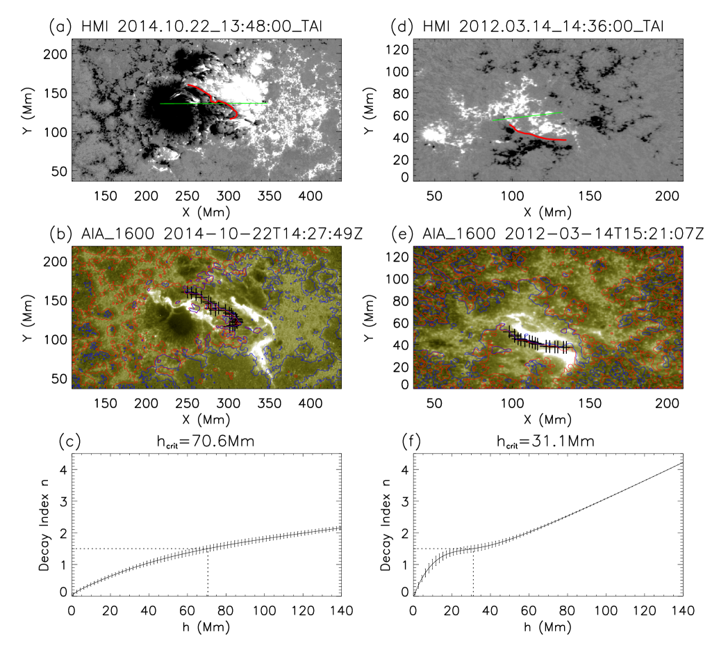
Figure 1: Derivation of the decay index profile for two exemplary events, a confined flare (No. 52) on the left and an eruptive flare (No. 12) on the right. (a) and (d) HMI $B_{z}$ map. The red line denotes the flaring PIL and the green line connects the centroids of opposite polarities. (b) and (e) The AIA 1600 Å image overlaid by $B_{z}$ contour (50 G and 10 G), with red (blue) colors indicating negative (positive) polarity. The sign ‘+’ denotes the points selected along the flaring PIL. (c) and (f) The decay index $n$ as a function of the height $h$ above the surface in units of Mm. Dotted lines indicate where $n_{\mathrm{crit}}$ and $h_{\mathrm{crit}}$ are taken.

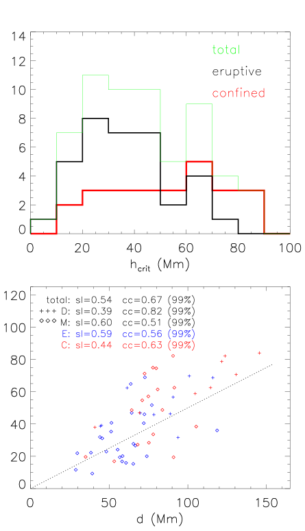
Figure 2: Distribution of $h_{\mathrm{crit}}$ (top) and its relation to the centroid distance $d$ of active regions (bottom). In the bottom panel, plus and diamond symbols denote dipolar (D) and multipolar (M) magnetic field, respectively. Eruptive (‘E’) and confined (‘C’) events are shown in blue and red, respectively. ‘sl’ indicates the slope given by linear fitting and ‘cc’ the correlation coefficient with the confidence interval denoted in the brackets. $h_{\mathrm{crit}}=\frac{1}{2}d$ is marked by the dotted line.

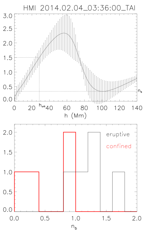
Figure 3: Saddle-like $n(h)$ profile. Top panel shows an exemplary $n(h)$ profile from the confined flare on 2014 February 4 (No. 48 in Table 1). $n_{b}$ and $h_{\mathrm{crit}}$ are marked. Bottom panel shows the distribution of $n_{b}$ for 5 eruptive (black) and 4 confined (red) flares.

References

- Alissandrakis (1981) Alissandrakis, C. E. 1981, A&A, 100, 197
- Aulanier et al. (2010) Aulanier, G., Török, T., Démoulin, P., & DeLuca, E. E. 2010, ApJ, 708, 314
- Bobra et al. (2014) Bobra, M. G., Sun, X., Hoeksema, J. T., et al. 2014, Sol. Phys., 289, 3549
- Cheng et al. (2011) Cheng, X., Zhang, J., Ding, M., Guo, Y., & Su, J. 2011, The Astrophysical Journal, 732, 87
- Démoulin & Aulanier (2010) Démoulin, P., & Aulanier, G. 2010, ApJ, 718, 1388
- Fan & Gibson (2007) Fan, Y., & Gibson, S. E. 2007, ApJ, 668, 1232
- Harrison (2003) Harrison, R. 2003, Advances in Space Research, 32, 2425
- Kliem et al. (2014) Kliem, B., Lin, J., Forbes, T. G., Priest, E. R., & Török, T. 2014, ApJ, 789, 46
- Kliem et al. (2013) Kliem, B., Su, Y. N., van Ballegooijen, A. A., & DeLuca, E. E. 2013, ApJ, 779, 129
- Kliem & Török (2006) Kliem, B., & Török, T. 2006, Physical Review Letters, 96, 255002
- Lemen et al. (2011) Lemen, J. R., Akin, D. J., Boerner, P. F., et al. 2011, in The Solar Dynamics Observatory (Springer), 17–40
- Liu et al. (2015) Liu, C., Deng, N., Liu, R., et al. 2015, ApJ, 812, L19
- Liu et al. (2016a) Liu, L., Wang, Y., Wang, J., et al. 2016a, ApJ, 826, 119
- Liu et al. (2016b) Liu, R., Chen, J., Wang, Y., & Liu, K. 2016b, Scientific Reports, 6, 34021
- Liu et al. (2010) Liu, R., Liu, C., Wang, S., Deng, N., & Wang, H. 2010, ApJ, 725, L84
- Liu et al. (2016) Liu, R., Kliem, B., Titov, V. S., et al. 2016, The Astrophysical Journal, 818, 148
- Liu (2008) Liu, Y. 2008, The Astrophysical Journal Letters, 679, L151
- Myers et al. (2015) Myers, C. E., Yamada, M., Ji, H., et al. 2015, Nature, 528, 526
- Myers et al. (2016) —. 2016, Physics of Plasmas, 23, 112102
- Myers et al. (2017) —. 2017, Plasma Physics and Controlled Fusion, 59, 014048
- Pesnell et al. (2012) Pesnell, W. D., Thompson, B. J., & Chamberlin, P. C. 2012, Sol. Phys., 275, 3
- Priest & Forbes (2002) Priest, E., & Forbes, T. 2002, The Astronomy and Astrophysics Review, 10, 313
- Scherrer et al. (2012) Scherrer, P. H., Schou, J., Bush, R., et al. 2012, Solar Physics, 275, 207
- Shibata (1998) Shibata, K. 1998, Astrophysics and Space Science, 264, 129
- Sun et al. (2015) Sun, X., Bobra, M. G., Hoeksema, J. T., et al. 2015, The Astrophysical Journal Letters, 804, L28
- Sun et al. (2015) Sun, X., Bobra, M. G., Hoeksema, J. T., et al. 2015, ApJ, 804, L28
- Titov & Démoulin (1999) Titov, V., & Démoulin, P. 1999, Astronomy and Astrophysics, 351, 707
- Török & Kliem (2005) Török, T., & Kliem, B. 2005, ApJ, 630, L97
- Török & Kliem (2007) Török, T., & Kliem, B. 2007, Astronomische Nachrichten, 328, 743
- van Tend & Kuperus (1978) van Tend, W., & Kuperus, M. 1978, Sol. Phys., 59, 115
- Wang et al. (2017) Wang, W., Liu, R., Wang, Y., et al. 2017, Nature Communications, under review
- Wang & Zhang (2007) Wang, Y., & Zhang, J. 2007, The Astrophysical Journal, 665, 1428
- Xu et al. (2012) Xu, Y., Liu, C., Jing, J., & Wang, H. 2012, The Astrophysical Journal, 761, 52
- Yashiro et al. (2005) Yashiro, S., Gopalswamy, N., Akiyama, S., Michalek, G., & Howard, R. A. 2005, Journal of Geophysical Research (Space Physics), 110, A12S05
- Zhang et al. (2001) Zhang, J., Dere, K., Howard, R., Kundu, M., & White, S. 2001, The Astrophysical Journal, 559, 452
- Zhang et al. (2004) Zhang, J., Dere, K., Howard, R., & Vourlidas, A. 2004, The Astrophysical Journal, 604, 420
- Zuccarello et al. (2016) Zuccarello, F., Aulanier, G., & Gilchrist, S. 2016, The Astrophysical journal letters, 821, L23
- Zuccarello et al. (2015) Zuccarello, F. P., Aulanier, G., & Gilchrist, S. A. 2015, ApJ, 814, 126
- Zuccarello et al. (2014) Zuccarello, F. P., Seaton, D. B., Mierla, M., et al. 2014, The Astrophysical Journal, 785, 88