Hydrodynamic Photoevaporation of Protoplanetary Disks with Consistent Thermochemistry

Abstract

Photoevaporation is an important dispersal mechanism for protoplanetary disks. We conduct hydrodynamic simulations coupled with ray-tracing radiative transfer and consistent thermochemistry to study photoevaporative winds driven by ultraviolet and X-ray radiation from the host star. Most models have a three-layer structure: a cold midplane, warm intermediate layer, and hot wind, the last having typical speeds $\sim 30~{}{\rm km\ s^{-1}}$ and mass-loss rates $\sim 10^{-9}~{}M_{\odot}~{}{\rm yr}^{-1}$ when driven primarily by ionizing UV radiation. Observable molecules including $\mathrm{CO}$, $\mathrm{OH}$ and $\mathrm{H_{2}O}$ re-form in the intermediate layer and survive at relatively high wind temperatures due to reactions being out of equilibrium. Mass-loss rates are sensitive to the intensity of radiation in energy bands that interact directly with hydrogen. Comparison with previous works shows that mass loss rates are also sensitive to the treatment of both the hydrodynamics and the thermochemistry. Divergent results concerning the efficiency of X-ray photoevaporation are traced in part to differing assumptions about dust and other coolants.

1. Introduction

Protostellar/protoplanetary disks (hereafter PPDs) surrounding low-mass T Tauri stars are the birthplaces of planets and have typical lifetimes $\sim 10^{6}-10^{7}\ {\rm yr}$ lifespan (e.g. 1995Natur.373..494Z; 2001ApJ...553L.153H). Along with accretion onto the star, sequestration of mass in planets, and perhaps magnetized disk winds, photoevaporation by hard photons likely contributes to the dispersal of PPDs (1994ApJ...428..654H).

Hard photons in different energy bands experience different microscopic physics and have differing effects on PPDs. Following 2009ApJ...690.1539G, we use the term “far-UV (FUV)” for photon energies $6~{}{\rm eV}<h\nu<13.6~{}{\rm eV}$, “extreme-UV (EUV)” for $13.6~{}{\rm eV}<h\nu<0.1~{}{\rm keV}$, and “X-ray” for $h\nu>0.1~{}{\rm keV}$. While EUV may be blocked by the wind from the disk surface (e.g. 2005MNRAS.358..283A), FUV and X-ray radiation are more penetrating. All of these heat, dissociate, or ionize the gas via a plethora of mechanisms. In order to model photoevaporation of PPDs, therefore, one is required to take the richness of the microphysics into account, as well as its interaction with the hydrodynamics.

Evolving a hydrodynamic system coupled with thermochemistry to (quasi-) steady state could be prohibitively expensive if a large chemical reaction network were included. Past work on PPD photoevaporation has compromised (at least) one of the two aspects: hydrodynamics or thermochemistry. 2006MNRAS.369..216A; 2006MNRAS.369..229A modeled EUV photoevaporation in hydrodynamic simulations with minimum thermochemistry. On the other hand, calculations with detailed thermochemistry usually adopt semi-analytic prescriptions for the wind mass-loss rate rather than simulate multidimensional hydrodynamics e.g. 2008ApJ...683..287G; 2009ApJ...690.1539G (hereafter GH08, GH09). Some recent works conduct hydrodynamic simulations with interpolation tables for gas temperature drawn from hydrostatic scenarios (e.g. 2010MNRAS.401.1415O). More recently, 2012MNRAS.420..562H, 2016MNRAS.463.3616H, and 2017MNRAS.468L.108H have coupled hydrodynamics and thermochemistry in simulations of externally irradiated disks and pre-stellar cores; their code is three-dimensional, but their applications have been confined mostly to simplified geometries (spherical or cylindrical) for easier comparison to semi-analytic work.

This work focuses on a consistent combination of hydrodynamic simulation with a moderate-scale chemical network (24 species, $\sim 10^{2}$ reactions). We include the species and reactions that are relevant to photoevaporation, especially heating and cooling mechanisms. Full hydrodynamic simulations are carried out in 2.5-dimensions (axisymmetry), coupled with radiation, thermodynamics, and chemistry, by solving time-dependent differential equations in every zone throughout the simulation domain. Compared to simulations with interpolation tables for thermochemistry, this approach is able to deal with non-equilibrium processes, as when some chemical and hydrodynamic timescales are comparable. The long-term goal of our exploration is to predict observables, especially emission and absorption-line profiles and strengths of important atomic and molecular species, thereby constraining our wind models and the parameters that go into them (e.g. abundances, dust properties, EUV luminosities). We aim eventually to incorporate MHD processes, and expect that the combination of photoevaporative and magnetic effects will lead to higher mass-loss rates than each process acting alone. The hydrodynamic simulations presented here are first steps toward these goals.

This paper is structured as follows. In §2, we briefly summarize our numerical methods and physical approximations. Additional details concerning our treatment of thermochemical processes are given in the Appendices. §3 introduces the parameter choices underlying our fiducial model. §4 presents the main results of our calculations for this model, and for several other models that differ from the fiducial one in one or more parameters, with the goal of exploring the effects of these parameters on gross properties of the flow, especially the mass-loss rate. In §LABEL:sec:discussions, we discuss the role that different bands of radiation play, and also compare and contrast our results with those of 2009ApJ...690.1539G and 2010MNRAS.401.1415O. §LABEL:sec:conclusion concludes and summarizes the paper.

2. Methods

This section summarizes our methods. The computational scheme for hydrodynamics is first described, followed by our methods for radiative transfer and thermochemistry.

2.1. Hydrodynamics

Our modeling of PPD photoevaporation systems involves full hydrodynamic calculations. We use the grid-based, general-purpose, astrophysical code Athena++ (2016ApJS..225...22W; Stone et al., in preparation) in spherical coordinates $(r,\theta,\phi)$ but neglect all dependence on $\phi$: our simulations are axisymmetric. Magnetic fields are neglected in the present work, although Athena++ is fully capable of MHD (indeed optimized for it). We use the HLLC Riemann solver and van Leer reconstruction with improved order of accuracy using the revised slope limiter (see 2014JCoPh.270..784M). Consistent Multi-fluid Advection (CMA) is used to ensure strict conservation of chemical elements and species (e.g. 2010MNRAS.404....2G).

2.2. Radiative transfer

Absorption processes dominate scattering for most of the radiation that we consider: FUV, EUV, and $1~{}\mathrm{keV}$ X-rays (Draine_book; Verner+etal1996). An exception would be $\text{Ly}\alpha$ photons, which may dominate the FUV luminosity, and whose scattering into nonradial directions helps them to penetrate more deeply into the disk (e.g. 2011ApJ...739...78B). We find, however, that unscattered soft FUV photons penetrate the intermediate layer anyway, and more deeply than $\text{Ly}\alpha$. Like $\text{Ly}\alpha$, these photons dissociate $\mathrm{H_{2}O}$ and $\mathrm{OH}$, which can be important coolants, but not $\mathrm{H_{2}}$ or $\mathrm{CO}$(e.g. 1978ApJ...224..841S). The scattering of harder X-rays can be important for ionization and hence magnetic coupling of the upper layers of the disk (Igea+Glassgold1999; Bai+Goodman2009, e.g.), but we are neglecting magnetic fields here.

Therefore, in this paper, scattering is neglected, and radiative transfer consists only of radial ray tracing, the sources of all hard photons being assumed to lie at the origin ($r=0$). This is facilitated by our choice of spherical coordinates, although our algorithm can trace rays in nonradial directions also (Wang 2017, in preparation).

One ray is assigned to each radial column. Its luminosity is adjusted as it propagates through each cell according to the photoreactions within that cell. Some cells can be individually optically thick. Hence for photochemistry, we adopt as the effective flux at photon frequency $\nu$,

$$F_{\mathrm{eff}}(\nu)=F_{0}(\nu)\left\{\dfrac{1-\exp[-\delta l/\lambda(\nu)]}{\delta l/\lambda(\nu)}\right\}\ ,$$ (1)

where $F_{0}$ is the flux impinging on the inner face of the current cell, $\lambda(\nu)$ is the local absorption mean free path of photons at frequency $\nu$, and $\delta l$ is the chord length of the ray across the cell. (For radial ray tracing, $\delta l$ is simply the radial width of the cell.) Eq. (1) yields $F_{\mathrm{eff}}\rightarrow F_{0}$ as $(\delta l/\lambda)\rightarrow 0$.

2.3. Chemistry and Thermodynamics

In each cell, a coupled set of ordinary differential equations (ODEs) is solved to update the abundances of all $\mathcal{N}$ chemical species $\{n^{i}\}$ and internal energy density $\epsilon$. These equations read, nominally,

$$\begin{split}\dfrac{\mathrm{d}n^{i}}{\mathrm{d}t}&=\mathcal{A}^{i}_{\;jk}n^{j}n^{k}+\mathcal{B}^{i}_{\;j}n^{j}\ ;\\ \dfrac{\mathrm{d}\epsilon}{\mathrm{d}t}&=\Gamma-\Lambda\ ;\end{split}$$ (2)

in which the terms involving $\{\mathcal{A}^{i}_{\;jk}\}$ describe two-body reactions, while those in $\{\mathcal{B}^{i}_{\;j}\}$ represent photoionization and photodissociation. $\Gamma$ and $\Lambda$ are the heating and cooling rates per unit volume, respectively. $\{\mathcal{A}^{i}_{\;jk}\}$, $\Gamma$ and $\Lambda$ are usually functions of temperature $T$. The thermal energy density $\epsilon=c_{V}(\{n^{i}\})T$, where $c_{V}$ is the heat capacity of the gas at constant volume. (Thermochemistry and hydrodynamics are solved in separate substeps, whence we use $c_{V}$ instead of $c_{P}$ here.) The ODEs (2) are solved in conjunction with the hydrodynamics by operator splitting. That is, they are advanced one time step after each hydrodynamic step, which has included advection of the chemical species, while holding the masses of all elements fixed within each cell. Photoreactions are included using the radiative fluxes computed as described in §2.2. The updated internal energy $\epsilon$ and number densities $\{n^{i}\}$ of all species are then used to initialize the next hydrodynamic step.

The ODEs (2) are usually stiff and hence numerically difficult. We use a standard ODE solver with adaptive implicit modules, CVODE (see hindmarsh2005sundials). The solution of these equations dominates our total computation time, typically by a factor $\gtrsim 10$ compared to the hydrodynamics. Nonetheless, this brute-force approach rewards us by being able to deal with non-equilibrium conditions, as will be discussed later in this paper.

Guided by GH08, GH09, and our own numerical experiments, we adopt 24 species that are most relevant to heating and cooling processes involved in PPD photoevaporation: $\mathrm{e}^{-}$ (free electrons), $\mathrm{H}^{+}$, H, $\mathrm{H_{2}}$, $\mathrm{\mathrm{H_{2}}}^{*}$ (using the $v=6$ vibrational state as a proxy for $\mathrm{H_{2}}$ in all excited states, see Appendix A.1 and TH85), He, $\mathrm{He}^{+}$, O, $\mathrm{O}^{+}$, $\mathrm{O}^{*}$ (the ${}^{1}D$ state of atomic oxygen as a proxy for all neutral excited states, see Appendix A.2), OH, $\mathrm{H_{2}O}$, C, $\mathrm{C}^{+}$, CO, S, $\mathrm{S}^{+}$, Si, $\mathrm{Si}^{+}$, Fe, $\mathrm{Fe}^{+}$, Gr, $\mathrm{Gr}^{+}$, $\mathrm{Gr}^{-}$. Here Gr and Gr^± denote neutral and singly-charged dust grains, respectively.

We extract the reactions involving these species from the UMIST astrochemistry database (UMIST2013). However, the interstellar radiation fields and matter densities to which the standard UMIST database is usually applied are rather different from those of PPDs. We therefore exclude all reactions involving photons and dust grains in the UMIST library; instead, we evaluate those reaction rates separately.

Photoionization and photodissociation are critical mechanisms that affect photoevaporation. At each photon energy, the ionization cross section of each atomic species is evaluated using the data in Verner+Yakovlev1995; Verner+etal1996. For molecular species that can react with FUV photons, namely $\mathrm{H_{2}}$, CO, OH, and $\mathrm{H_{2}O}$ here, we adopt the FUV-induced photochemcial reaction rate based on 1985ApJ...291..722T for $\mathrm{H_{2}}$, 2009A&A...503..323V for CO (note that this photodissociation cross section is $\sim 10\times$ the value in TH85), and 2014ApJ...786..135A for $\mathrm{H_{2}O}$ and OH. The photochemical processes related to $\mathrm{H_{2}}$, C and CO may be subject to considerable self-shielding and cross-shielding. Using the radial column density data that are obtained by integrating along radial rays, we evaluate the impact of the self-/cross-shielding by adopting the analytic formulae in 2009A&A...503..323V (for CO) and TH85 (for C), and 1996ApJ...468..269D (for $\mathrm{H_{2}}$). It is worth noting that the FUV-induced processes in parallel with photodissociation of $\mathrm{H_{2}}$, $\mathrm{H_{2}O}$ and OH, e.g. FUV pumping of $\mathrm{H_{2}}$ onto its excited states and its subsequent effects, can have considerable thermodynamic effects. We refer the reader to Appendices A.1 and A.2 for detailed discussion.

Heating and cooling processes are directly associated with chemical reactions. While the amount of energy deposited into and removed from the gas by photoionization and recombination can be estimated straightforwardly (see also Draine_book, eqs. 27.3, 27.23), the thermodynamic effects of other chemical reactions need elaboration, which is provided in Appendices A.1 through A.3. There are other radiative mechanisms that remove energy from the gas, especially collisionally pumped ro-vibrational transitions of molecules, and fine-structure transitions of atoms. We briefly summarize those mechanisms and our method for evaluating them in Appendix A.4.

Dust grains are usually crucial in PPD photoevaporation. Following the arguments in GH08, as well as 2006A&A...459..545G; 2007A&A...476..279G; 2011ApJ...727....2P, we suggest that polycyclic aromatic hydrocarbons (PAHs) overwhelm dust grains of other sizes in terms of the following effects, thanks to their dominant contribution to total dust surface area: photoelectric heating of gas, dust-gas collisional energy transfer, recombination with free electrons, dust-assisted molecular hydrogen formation, and neutralization of positive ions. We include the processes listed above as outlined in Appendix A.3.

3. Choice of Fiducial model

This section presents the setup of our fiducial model, whose main properties are listed in Table 1. Other models, each differing from the fiducial in one parameter, are described in §4.2.

The simulation domain is axisymmetric, extending from $2~{}\,\mbox{\sc au}$ to $100~{}\,\mbox{\sc au}$ in radius ($r$) and $0$ to $\pi/2$ in colatitude ($\theta$). All models are presumed to be symmetric about the equatorial plane, so that, for example, quoted mass-loss rates include outflows at $\theta>\pi/2$. All dependence on the azimuthal coordinate ($\phi$) is ignored. Outflow boundary conditions with a radial flow limiter (which inhibits radial inflow) are imposed at $r=2~{}\,\mbox{\sc au}$ and $r=100~{}\,\mbox{\sc au}$, and reflecting boundary conditions at $\theta=0$ and $\theta=\pi/2$. Our standard resolution is $256$ radial by $128$ latitudinal zones, the radial zones being logarithmically spaced, and the latitudinal zones equally spaced.

The gravitational field is that of a $1~{}M_{\odot}$ star located at the origin. The disk, whose self-gravity is neglected, is initialized in hydrostatic and centrifugal balance, except for slight imbalances due to numerical discretization. The disk density and temperature profile follow the steady state solution in 2013MNRAS.435.2610N, in which we set the midplane density as $n=10^{10}~{}{\rm cm}^{-3}$ and temperature $T=20~{}{\rm K}$ at $r=10^{2}~{}\,\mbox{\sc au}$, with radial power index being $(-2.25)$ for density and $(-0.5)$ for temperature–this profile yields a disk mass $\approx 0.03M_{\odot}$ within $100~{}\,\mbox{\sc au}$. The density and temperature profiles roughly agree with GH09, but the latter are not quite hydrostatic.

All radiation emanates from the origin of spherical polar coordinates. Our simulation domain does not cover the origin, and the rays are not attenuated before they reach the inner boundary. The source is isotropic, but those rays that reach the midplane region at the inner boundary are discarded (we also test not discarding those rays, finding negligible differences in the dissociation layer and in the wind). Each ray has four discrete energy bins, representing four important bands of photon energy: $h\nu=7~{}{\rm eV}$ for FUV photons that do not interact appreciably with hydrogen molecules (“soft FUV” hereafter), $12~{}{\rm eV}$ for Lyman-Werner (“LW” for short) band photons, $25~{}{\rm eV}$ for EUV photons, and $1~{}{\rm keV}$ for X-ray photons. $\text{Ly}\alpha$ photons are neglected, as discussed above. The number of photons radiated in each energy bin per unit time follows the luminosity model described in GH08 and GH09: (1) a $9000~{}{\rm K}$ black body spectral profile for FUV ($6~{}{\rm eV}<h\nu<13.6~{}{\rm eV}$) with total luminosity $L_{\mathrm{FUV}}=10^{31.7}~{}{\rm erg}~{}{\rm s}^{-1}$; (2) an additional EUV-photon emission rate $\Phi_{\mathrm{EUV}}=10^{40.7}~{}{\rm s}^{-1}$; (3) and an X-ray luminosity $L_{X}=10^{30.4}~{}{\rm erg}~{}{\rm s}^{-1}$.

The initial elemental abundances are determined by the values in Table 1 (wherein $n_{\mathrm{H}}$ is the number density of hydrogen nuclei). These choices generally follow a subset of those in GH08, with the additional assumption that elements appear in chemical compounds if possible. These initial abundances are uniform throughout the simulation domain.

Our assumptions about the dust turn out to be important for our results. GH08 and GH09 treated two populations of grains: (i) an MRN-type power-law distribution with a minimum grain radius of $50~{}\mathrm{\AA}$, maximum of $20~{}{\rm\mu m}$, and a dust-to-gas ratio by mass of $10^{-2}$; and (ii) PAH grains with abundance $8.4\times 10^{-8}$ per hydrogen nucleus. The first population has a total geometrical cross section of $2\times 10^{-22}~{}{\rm cm}^{2}$ per hydrogen nucleus ($\sigma_{\rm dust}/\mathrm{H}$). The authors do not state the radius of their PAH grains explicitly, but they refer to 2001ApJ...554..778L, and we interpret this to mean that their PAHs can be approximated by spheres of radius $6~{}\mathrm{\AA}$. It would follow that the contribution of their PAHs to the cross section is $\sigma_{\rm dust}/\mathrm{H}\approx 9.5\times 10^{-22}$, i.e. several times larger than that of their MRN population, although the contribution to the dust-to-gas mass ratio is only $\sim 10^{-4}$. As noted above, A.3, the principal effects of dust, especially heating and absorption of radiation, are expected to be dominated by the smallest grains—PAHs.

For simplicity, we prefer to work with a single-sized grain population. We therefore neglect MRN grains and take the approximate relative abundance for our PAH-like grain species (Gr) as $10^{-7}$ per hydrogen atom, slightly greater than that of GH08, and a PAH radius of $5~{}\mathrm{\AA}$, i.e. approximately $60$ carbon atoms per PAH: see 2001ApJS..134..263W). The dust-to-gas mass ratio is then $0.7\times 10^{-4}$, and $\sigma_{\rm dust}/\mathrm{H}=8\times 10^{22}~{}{\rm cm}^{2}$.

Although variable dust abundance is fully allowed by our code, for the sake of simplicity we set the relative abundance of Gr to be uniform and assume that the dust comoves with the gas.

We run the simulation for $1.2\times 10^{4}~{}{\rm yr}$ with microphysics enabled but the central radiation sources turned off until the disk structure is fully numerically relaxed, and the temperature profile converges to that set by the artificial heating profile (§A.3.3, which is sufficiently close to the initial profile. The chemical abundances do not change during this relaxation process except by passive advection. We confirm after this process that the disk is indeed in hydrodynamic equilibrium and has no outflow. Then, at $t=3.6\times 10^{3}~{}{\rm yr}$, irradiation is turned on and remains on for the rest of simulation; this lasts $\gtrsim 500~{}{\rm yr}$, sufficiently long compared to the radial flow timescale $\tau\sim(100~{}\,\mbox{\sc au})/(30~{}{\rm km\ s^{-1}})\approx 16~{}{\rm yr}$ so as to reach an approximate quasi-steady state. On Princeton University’s local computer cluster perseus, $500~{}{\rm yr}$ of simulated time takes $\sim 100~{}\mathrm{\ hrs}$ of wall-clock time on 128 CPUs. About 95 per cent of the time is consumed by the thermochemical calculations for the fiducial model, the hydrodynamic and ray-tracing steps being relatively quick.

Table 1Properties of the fiducial model

Item	Value
Radial domain	$2~{}\,\mbox{\sc au}\leq r\leq\ 100~{}\,\mbox{\sc au}$
Latitudinal domain	$0\leq\theta\leq\pi/2$
Resolution	$N_{\log r}=256$, $N_{\theta}=128$
Stellar mass	$1.0~{}M_{\odot}$
$M_{\mathrm{disk}}$	$0.03~{}M_{\odot}$
Mid-plane density	$10^{10}(R/100~{}\,\mbox{\sc au})^{-2.25}~{}{\rm cm}^{-3}$
Mid-plane temperature	$20(R/100~{}\,\mbox{\sc au})^{-0.5}~{}{\rm K}$
Luminosities [photon ${\rm s}^{-1}$]
$7~{}{\rm eV}$ (“soft” FUV)	$4.5\times 10^{42}$
$12~{}{\rm eV}$ (LW)	$1.6\times 10^{40}$
$25~{}{\rm eV}$ (EUV)	$5.0\times 10^{40}$
$1~{}{\rm keV}$ (X-ray)	$1.6\times 10^{39}$
Initial abundances [$n_{\mathrm{X}}/n_{\mathrm{H}}$]
$\mathrm{H_{2}}$	0.5
He	0.1
$\mathrm{H_{2}O}$	$1.8\times 10^{-4}$
CO	$1.4\times 10^{-4}$
S	$2.8\times 10^{-5}$
Si	$1.7\times 10^{-6}$
Fe	$1.7\times 10^{-7}$
Gr	$1.0\times 10^{-7}$
Dust/PAH properties
$r_{\mathrm{dust}}$	$5~{}\mathrm{\AA}$
$\rho_{\mathrm{dust}}$	$2.25~{}{\rm g}~{}{\rm cm}^{-3}$
$m_{\mathrm{dust}}/m_{\mathrm{gas}}$	$7\times 10^{-5}$
$\sigma_{\mathrm{dust}}/\mathrm{H}$	$8\times 10^{22}~{}{\rm cm}^{2}$

We also calculate several models that differ from the fiducial in one or more parameters, as described in §4.2.

4. Results

In this section, we first present and elaborate the fiducial simulation (see §3), then compare the the results of the variant models shown in 2 (see §4.2).

4.1. Fiducial Model

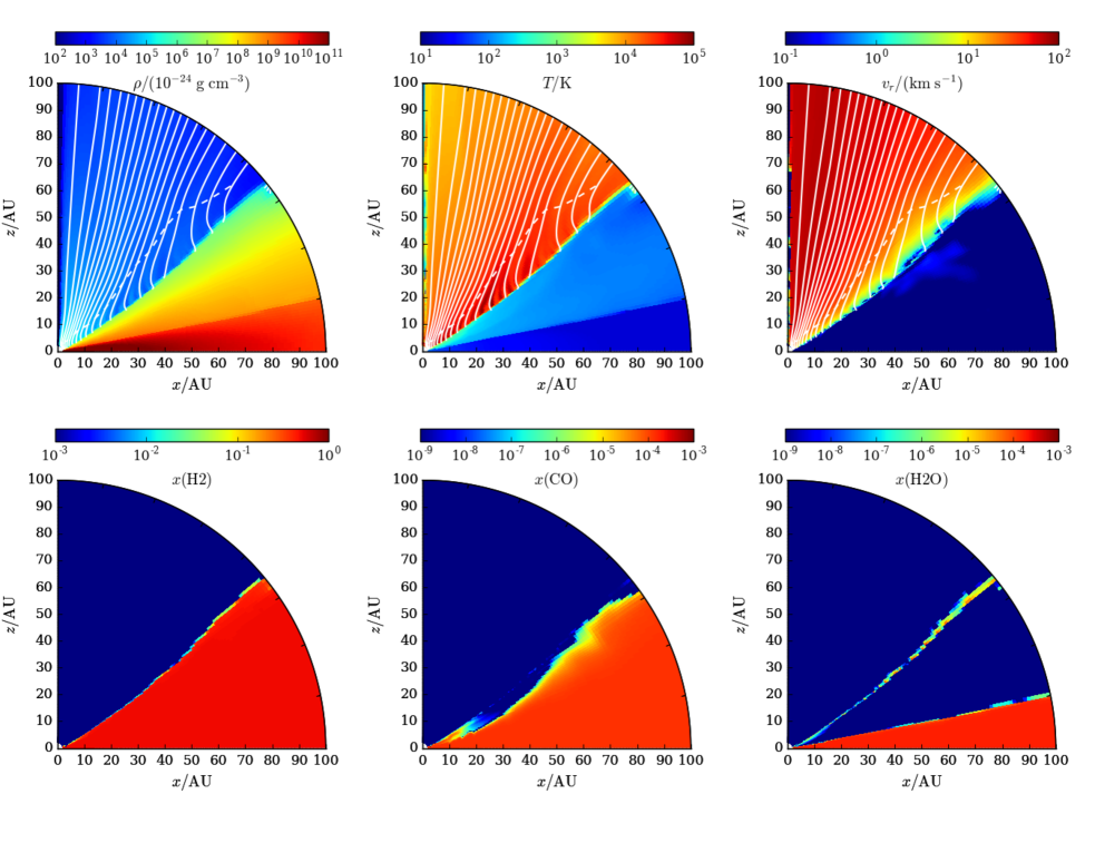
Figure 1.— Meridional plots for the fiducial model (§3), averaged through the final $100~{}{\rm yr}$ of the simulation. Top row: basic hydrodynamic profiles; left panel: mass density in units of $10^{-24}~{}{\rm g}~{}{\rm cm}^{-3}$; middle panel: temperature in Kelvin; right panel: radial velocity in ${\rm km\ s^{-1}}$. Panels in the top row are overlapped by streamlines (white solid lines), separated by $10^{-10}~{}M_{\odot}~{}{\rm yr}^{-1}$ wind mass loss rate (see §4.1 for details), and the locations of sonic points (white dashed line). Bottom row: relative abundance of different species [in units of $n(\mathrm{X})/n_{\mathrm{H}}$]; left panel: $\mathrm{H_{2}}$; middle panel: $\mathrm{CO}$; right panel: $\mathrm{H_{2}O}$.

Fig. 1 displays meridional plots of the structure of our fiducial model averaged over the final $100~{}{\rm yr}$ of the simulation. The white curves shown in the top row of panels are streamlines, the integral curves of the vector field $\rho\boldsymbol{v}_{p}$ ($\boldsymbol{v}_{p}$ is the poloidal velocity), spaced by constant mass-loss rate $10^{-10}~{}M_{\odot}~{}{\rm yr}^{-1}$: that is to say, this is the mass flux between neighboring streamlines when integrated over azimuth and multiplied by two to include the reflection of the computational region below the equatorial plane. Streamlines that meet the outer boundary with a negative value of the Bernoulli parameter

$$\mathcal{B}\equiv\dfrac{v^{2}}{2}+\dfrac{\gamma p}{(\gamma-1)\rho}+\Phi\ ,$$ (3)

are not plotted, and the outflow along such streamlines is omitted from the computation of the total mass-loss rate. Here $v$ is the magnitude of fluid velocity vector, $p$ the gas pressure, $\gamma\approx 5/3$ the adiabatic index, and $\Phi$ the gravitational potential. With this mask we get rid of (very slow) radial flows near the mid-plane: since the density there is six orders of magnitude higher than the wind, a tiny radial velocity fluctuation could otherwise give a spurious contribution to the mass-loss rate. As displayed in Fig. 1, the streamlines terminate on the disk at the surface where $\mathcal{B}$ becomes negative. We consider this surface to be the base of the wind. (As discussed in §LABEL:sec:GH09_comparison, this definition of the wind base differs from that of GH09.)

Fig. 2 shows several flow variables along two representative streamlines originating from cylindrical radii $R\equiv r\sin\theta=5~{}\,\mbox{\sc au}$ and $R=15~{}\,\mbox{\sc au}$.

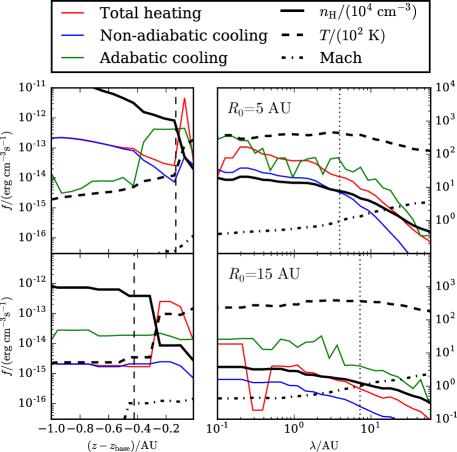
Figure 2.— Cooling/heating rates (left ordinate) and fluid properties (right ordinate) along streamlines. $n_{\mathrm{H}}$ is the number density of hydrogen nuclei. In right column, horizontal axis is arc length ($\lambda$) measured from the wind base [where $\mathcal{B}=0$, eq. (3)]. Vertical dotted line marks sonic point. Left column present the profile vertically below wind base (i.e. $z-z_{\mathrm{base}}$). Vertical dashed line indicates wind base as defined by GH09. Upper row: streamline rooted at $R_{0}=5~{}\,\mbox{\sc au}$. Lower row: $R_{0}=15~{}\,\mbox{\sc au}$.

The density and temperature profiles shown by Fig. 1 can be divided into three relatively distinct regions:

• Midplane layer: $0<(z/R)\lesssim 0.3$ ($R=r\sin\theta$ being cylindrical radius), $T<10^{2}{\rm K}$. The structure here is basically unchanged from the initial conditions.

• Intermediate layer: $0.3\lesssim(z/R)\lesssim 0.6$, $10^{-19}~{}{\rm g}~{}{\rm cm}^{-3}\lesssim\rho\lesssim 10^{-16}~{}{\rm g}~{}{\rm cm}^{-3}$, $10^{2}\lesssim T\lesssim 10^{3}~{}{\rm K}$. The total mass in this layer is $\sim 10^{-6}~{}M_{\odot}$. EUV photons scarcely penetrate this region, whose properties are controlled by FUV and X-ray processes: photodissociation and photoelectric heating, as well as radiative cooling by collisionally excited molecular and/or atomic transitions. Most $\mathrm{H_{2}}$ molecules and a lot of $\mathrm{CO}$ molecules survive in this region because of significant self- and cross-shielding of Lyman-Werner photons. Soft FUV photons that do not interact much with molecular hydrogen are relatively unshielded and pervade the intermediate layer, photodissociating $\mathrm{OH}$ and $\mathrm{H_{2}O}$), penetrating to the bottom of the layer, or escaping through the outer radial boundary.

• Wind layer: $(z/R)\gtrsim 0.6$, $\rho\lesssim 10^{-19}~{}{\rm g}~{}{\rm cm}^{-3}$, $T\gtrsim 10^{4}~{}{\rm K}$. This region is filled with mostly ionized gas, flowing outwards at radial velocity $v_{r}\sim 30~{}{\rm km\ s^{-1}}$. Photoionization heating and adiabatic expansion dominate the thermodynamics of this region.

Figure 3.— Variation of mass-loss rate measured at the $r=100~{}\,\mbox{\sc au}$ outer boundary of the fiducial model (Model 0). The dashed horizontal line shows the average of mass-loss rate over the last $200~{}{\rm yr}$.

If we integrate the $\mathcal{B}$-masked radial mass flux at the the $r=100~{}\,\mbox{\sc au}$ boundary (and its reflection at $z<0$) and average over the last $100~{}{\rm yr}$ of our fiducial run, we obtain a total mass-loss rate $\dot{M}_{\mathrm{wind}}\simeq 3.4\times 10^{-9}~{}M_{\odot}~{}{\rm yr}^{-1}$, corresponding to a disk dispersal timescale $\sim 10^{7}~{}{\rm yr}$. The mass-loss rate is lower than that of GH09 (see §LABEL:sec:GH09_comparison for further discussion). However, our mass-loss rate undergoes significant fluctuations, and is uncertain to at least $\sim 10$ per cent. Fig. 3 plots the mass-loss rate for the last $200~{}{\rm yr}$ of the (lower resolution) fiducial run (Model 0). They correlate with what appears to be a thermal instability of the outer disk, whereby it swells vertically, intercepts more radiation, and then swells further but also migrates at a few ${\rm km\ s^{-1}}$ through the outer boundary, temporarily increasing $\dot{M}$. This behavior is smoothed over by the time averages used to make Fig. 1. These swellings, being slower and denser than the general wind, partly shield themselves against photodissociation of some molecules, especially $\mathrm{H_{2}}$ and $\mathrm{CO}$, so that those molecules survive farther into the outflow than they would otherwise.

Even outside these swellings, there are also molecules surviving in regions with rather high temperature ($\sim 10^{3}~{}{\rm K}$, or even up to $\sim 10^{4}~{}{\rm K}$). $\mathrm{H_{2}O}$ and $\mathrm{OH}$ molecules exist at the surface of the intermediate layer, detached from the midplane (last panel of Fig. 1). The reformation rates of $\mathrm{H_{2}O}$ and $\mathrm{OH}$ are comparable to photodissociation at that surface. At the cooler temperatures below it, inside the intermediate layer, reformation is less efficient but photodissociating FUV is still present. The wind region, on the other hand, does not have sufficient $\mathrm{H_{2}}$ (reactions that are most efficient in forming $\mathrm{H_{2}O}$ and $\mathrm{OH}$ need $\mathrm{H_{2}}$ as reactants, while the reactions that convert atomic H to OH and $\mathrm{H_{2}O}$ are very slow).

In Fig. 4, we plot the distribution of $\mathrm{CO}$, $\mathrm{OH}$ and $\mathrm{H_{2}O}$ in the wind region and intermediate layer, in the plane of by $\log_{10}T$ and $v_{r}$. (The temperature $T$ here represents the kinetic temperature of the local (mostly $\mathrm{H}$ & $\mathrm{He}$) gas, not the vibrational or even rotational excitation temperature of the molecules.) For those molecules, a tail on the high temperature ($T\sim 10^{3}\mbox{--}10^{4}~{}{\rm K}$) and intermediate radial velocity ($v_{r}\sim 5\mbox{--}10~{}{\rm km\ s^{-1}}$) end of the 2-D distribution indicate their survival at the bottom in the wind region. Such hot molecular gas would be less prominent had we assumed local thermochemical equilibrium. For the luminosity in the LW and EUV bands of our fiducial model, it can be estimated that the timescale of CO photodissociation is $\sim 0.1~{}{\rm yr}$ at $r\sim 10~{}\,\mbox{\sc au}$. Given the speed of photoevaporative outflow, this timescale is sufficient for some CO to survive $\sim 0.1-1~{}\,\mbox{\sc au}$ into the hot wind. These timescales are sensitive to radial distance (from the radiation sources), to the way photodissociation is modeled (see §2.3), and to the LW and EUV band luminosity. Observational constraints on such molecules could be an important check on these models, and might diagnose the role of UV in driving PPD winds.

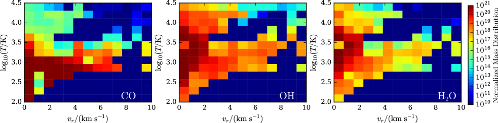
Figure 4.— Distribution functions of key molecular species based on the fiducial model (left panel: CO; middle panel: OH; right panel: $\mathrm{H_{2}O}$) in the two-dimensional space of $\{\log_{10}T\}\times\{v_{r}\}$ (common logarithm of temperature and radial velocity). The mass distribution function is normalized as $\mathrm{d}^{2}m/[\mathrm{d}\log_{10}(T/{\rm K})\mathrm{d}(v_{r}/{\rm km\ s^{-1}})]$, i.e. mass of the species per dex-temperature per $(v_{r}/{\rm km\ s^{-1}})$.

4.2. Exploring the Parameter Space

To explore the effects of our input parameters, we have run a number of additional simulations, most differing from the fiducial run in one parameter. These models and some synoptic results are listed in Table 2. We discuss some of these models here, and others in §§LABEL:sec:GH09_comparison-LABEL:sec:compare-oeca10 in relation to the works by GH09 and OECA10.

In the fiducial model the luminosity in the Lyman-Werner band is tiny compared to that in soft ($h\nu<11.3~{}{\rm eV}$) FUV photons: around 0.35 per cent, using the $9000~{}{\rm K}$ black body SED. However, as observed by e.g. 2000ApJ...544..927G, the SED for FUV radiation is rather variable from object to object and often more luminous in the LW band than the black-body model adopted by GH08 and GH09. Hence we include a series of models, with 0 and 100 times the fiducial luminosity in the Lyman-Werner band, to cover this uncertainty. We also test 0 and 10 times EUV or X-ray luminosity to diagnose the impact of those photons that can ionize atomic hydrogen.

For very small grains such as our PAHs, the grain absorption cross section for FUV and EUV photons depends on total grain mass rather than grain area. We have a much smaller grain mass than GH09. Model 9 in Table 2 has double the dust radius ($r_{\mathrm{dust}}=10~{}\mathrm{\AA}$) and therefore eight times the dust mass at the same relative number density ($n_{\mathrm{Gr}}/n_{\mathrm{H}}=10^{-7}$).

To test our truncation errors, we repeat the fiducial run at resolution $128\times 64$, i.e. coarser by $\times 2$ in both latitude and radius. This convergence test is run for much longer time period ($\sim 2000~{}{\rm yr}$) to better characterize fluctuations around the mean state.

Fig. 5 illustrates the hydrodynamic structure of a few representative models. These plots are based on time averages over $100~{}{\rm yr}$, so that the flow field is in approximate steady state. In the runs with $100\times$ LW photons (Model 2) or $10\times$ X-ray photons (Model 8), a thick neutral atomic layer exists at the top of the intermediate layer. In this layer, the temperature and sound speed reach a local maximum with respect to height or latitude, and significant outflows may occur. This causes the jagged shape of the sonic curves in the third and fourth panels.

Table 2Models exploring parameter space

No.	Description	$\dot{M}_{\mathrm{wind}}$	$\dot{M}_{\mathrm{GH}}$	Total heating	Efficiency	$\langle v_{r}\rangle$
		$(10^{-9}M_{\odot}~{}{\rm yr}^{-1})$	$(10^{-9}M_{\odot}~{}{\rm yr}^{-1})$	$(10^{30}{\rm erg}~{}{\rm s}^{-1})$		$({\rm km\ s^{-1}})$
(1)	(2)	(3)	(4)	(5)	(6)	(7)
0	Fiducial	2.5 $\pm$ 0.2	11.6	4.4	0.67	39
1	No LW photons	2.5 $\pm$ 0.3	9.3	4.1	0.67	38
2	100$\times$ LW photons	17.6 $\pm$ 2.1	61.3	9.1	0.60	18
3	No ”soft” FUV	1.1 $\pm$ 0.1	2.7	2.3	0.53	58
4	”Soft” FUV only	0.0	0.2	1.0	-	-
5	No EUV	0.0	3.7	1.6	-	-
6	10$\times$ EUV photons	9.4 $\pm$ 0.7	107.8	26.7	0.74	33
7	No X-ray	2.1 $\pm$ 0.2	6.9	2.6	0.80	38
8	10$\times$ X-ray photons	9.1 $\pm$ 0.4	55.6	14.1	0.42	24
9	$r_{\mathrm{dust}}=10~{}\mathrm{\AA}$	2.8 $\pm$ 0.6	10.5	3.5	0.68	30
10	$\mathrm{OECA10\ analog}^{\dagger}$	11.2 $\pm$ 4.2	105.0	0.8	0.54	5
11	Convergence test	2.7 $\pm$ 0.6	16.1	3.0	0.58	32

Note. — (1) Model identifier. (2) Parameter by which model differs from fiducial. (3) Wind mass-loss rate. The error quoted error is $\Delta\dot{M}_{\mathrm{wind}}=\langle[\dot{M}(t)]^{2}-\langle\dot{M}\rangle^{2}\rangle^{1/2}$, where the time averages are taken over the last $100~{}{\rm yr}$. (4) Estimated wind mass-loss rate using GH09 scheme. (5) Total radiative plus thermal-accomodation heating of the gas (note that the accomodation heating can be negative). (6) Thermal-to-mechanical conversion efficiency: (heating $-$ non-adiabatic cooling)$/$(heating). (7) Mean outflow velocity weighted by radial mass flux.

$\dagger$: Bernoulli parameter mask not applied; significant outflow occurs in the intermediate layer with $\mathcal{B}<0$.

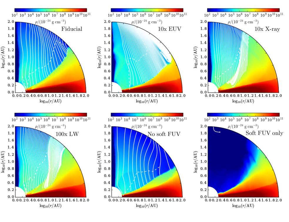
Figure 5.— Selected plots of streamlines (based on $100~{}{\rm yr}$ average), overlaid on density colormaps, that are relevant to the discussions in §4. The black curves, showing the streamlines, are separated by $10^{-10}~{}M_{\odot}~{}{\rm yr}^{-1}$ each. The white curves denote the location of sonic point of all streamlines plotted. Note that, for clearer presentation, the radial coordinates in all panels are $\log_{10}(r/\,\mbox{\sc au})$.

Figs. LABEL:fig:heating and LABEL:fig:cooling show the vertical distributions of heating and cooling mechanisms at $R=15~{}\,\mbox{\sc au}$, a typical location where the outflow streamlines originate. The three layer structure (§4.1) is obvious in most of the models. Details of those structures vary with model parameters, with implications for the mechanisms responsible.

The panels of Fig. LABEL:fig:heating convey some general impressions about the heating mechanisms. The vertical heating profile usually has two peaks: one at the bottom of the intermediate layer, the other at the top of it. Photoionization heating by the harder (EUV and X-ray) photons dominates, unless these photons are absent or are overwhelmed by photons in other bands (e.g. Model 2, $100\times$ LW photons; see discussions below). On the cooling side (Fig. LABEL:fig:cooling), the $\mathrm{OH}$ and/or $\mathrm{H_{2}O}$ ro-vibrational transitions and S I $25~{}{\rm\mu m}$ transition dominate at the bottom of intermediate layer, the Si II $35~{}{\rm\mu m}$ and O I $63~{}{\rm\mu m}$ transitions in the middle of that layer, and $\mathrm{H_{2}}$ ro-vibrational cooling near the top. In the “wind” region, cooling and heating are dominated by recombination and the photoelectric effect. Using the integrated cooling rate, we have estimated some of the important line luminosities (Table LABEL:table:line-luminosity).

Table 3Approximate line luminosity

Model	O I $63\ {\rm\mu m}$	O I $6300~{}\mathrm{\AA}$	S I $25\ {\rm\mu m}$	Si II $35\ {\rm\mu m}$	$\mathrm{H_{2}}$ ro-vib	$\mathrm{OH}$/$\mathrm{H_{2}O}$ ro-vib	$\mathrm{CO}$ ro-vib
0	$-4.31$	$-7.36$	$-4.00$	$-5.65$	$-4.67$	$-4.29$	$-3.89$
1	$-4.34$	$-8.17$	$-3.96$	$-5.73$	$-4.60$	$-4.36$	$-3.90$
2	$-3.75$	$-4.69$	$-4.17$	$-4.73$	$-4.11$	$-3.57$	$-3.91$
3	$-5.05$	$-7.72$	$-5.05$	$-6.48$	$-5.26$	$-3.61$	$-5.68$
4	$-5.05$	-	$-4.68$	-	$-5.61$	$-4.30$	$-4.26$
5	$-4.22$	$-7.31$	$-3.97$	$-5.58$	$-5.03$	$-4.63$	$-3.88$
6	$-4.43$	$-7.13$	$-3.88$	$-5.36$	$-3.65$	$-3.56$	$-3.78$
7	$-4.74$	$-8.02$	$-4.61$	$-6.30$	$-4.72$	$-4.26$	$-4.23$
8	$-3.57$	$-5.99$	$-3.11$	$-4.69$	$-4.15$	$-3.38$	$-3.37$
9	$-4.47$	$-4.94$	$-4.39$	$-5.94$	$-4.39$	$-4.07$	$-4.59$
10	$-4.38$	$-6.88$	-	$-4.55$	-	-	-
11	$-4.49$	$-5.24$	$-4.32$	$-5.98$	$-4.79$	$-4.94$	$-4.83$

Appendix A Details of Thermochemical processes

A.1. FUV induced reactions of $\mathrm{H_{2}}$

When a $13.6~{}{\rm eV}>h\nu>11.3~{}{\rm eV}$ photon (the “Lyman-Werner” band, or LW for short) encounters hydrogen molecules, this photon can be absrobed by a $\mathrm{H_{2}}$ molecule, and excite the $\mathrm{H_{2}}$ molecule into an excited electronic state. This state can spontaneously decay into different ro-vibrational states, hence we have to include the excited $\mathrm{\mathrm{H_{2}}}^{*}$ as a representative for excited molecular hydrogen. Such photo-pumping of $\mathrm{H_{2}}$ is also subject to self-shielding effects. We follow 1996ApJ...468..269D for the shielding factor.

As summarized by TH85, about 10 per cent of the excited hydrogen molecules result in photo-dissociation; we hereby simplify this reaction channel by adding a branch to the main photo-excitation channel, namely,

$$\mathrm{H_{2}}+h\nu(\mathrm{LW})\rightarrow\begin{cases}2\mathrm{H}\ ,\ &\sim 10\ \text{per cent}\ ;\\ \mathrm{\mathrm{H_{2}}}^{*}\ ,\ &\sim 90\ \text{per cent}\ .\\ \end{cases}$$

$\mathrm{\mathrm{H_{2}}}^{*}$ molecules may also be directly photo-dissociated; the reaction cross section of TH85 is adopted. We take 0.4 eV as the amount of energy deposited in the gas as heat per FUV dissociation of $\mathrm{H_{2}}$ (2016arXiv161009023G; see also 1979ApJS...41..555H).

At gas densities relevant here, the majority of excited hydrogen molecules are de-excited by collisions with other particles, especially $\mathrm{H_{2}}$ or H. The de-excitation rate (with the $v=6$ vibrational state as a proxy for all excited $\mathrm{\mathrm{H_{2}}}^{*}$), is estimated by (see also TH85),

$$\begin{split}k_{\mathrm{de}}(\mathrm{H})&\simeq 1.8\times 10^{-13}~{}{\rm cm}^{3}~{}{\rm s}^{-1}\times\left(\dfrac{T}{{\rm K}}\right)^{1/2}\exp\left(-\frac{1000~{}{\rm K}}{T}\right)\ ;\\ k_{\mathrm{de}}(\mathrm{H_{2}})&\simeq 2.3\times 10^{-13}~{}{\rm cm}^{3}~{}{\rm s}^{-1}\times\left(\frac{T}{{\rm K}}\right)^{1/2}\exp\left(-\frac{18000~{}{\rm K}}{T+1200~{}{\rm K}}\right)\ .\end{split}$$ (A1)

Each collisional de-excitation deposits $\sim 2.6~{}{\rm eV}$ of heat into the gas (see also TH85). The rate for spontaneous radiative de-excitation of $\mathrm{\mathrm{H_{2}}}^{*}$ is taken to be $A(\mathrm{\mathrm{H_{2}}}^{*})\simeq 2\times 10^{-7}~{}{\rm s}^{-1}$ (TH85).

A.2. FUV induced reactions of $\mathrm{H_{2}O}$ and $\mathrm{OH}$

Photodissociation of $\mathrm{H_{2}O}$ and $\mathrm{OH}$ is not drastically affected by self-/cross-shielding due to line overlap. For the photodissociation cross sections of these two species as functions of photon energy, we adopt Fig. 1 of AGN14. These reactions also heat the gas. Here we adopt the estimate in AGN14 that about $\sim 0.5(h\nu-E_{\mathrm{diss}})$ of heat is deposited into the gas per reaction, where $E_{\mathrm{diss}}(\mathrm{H_{2}O})\simeq 5.13~{}{\rm eV}$, and $E_{\mathrm{diss}}(\mathrm{OH})\simeq 4.41~{}{\rm eV}$. Photodissociation of $\mathrm{OH}$ may result in oxygen atoms in the ${}^{1}D$ state, denoted by $\mathrm{O}^{*}$, which spontaneously decays to the ${}^{3}P$ state while emitting a photon at $6300~{}\mathrm{\AA}$. Due to the uncertainty or variability of the FUV spectrum, we adopt the crude approximation that $\sim 55$ per cent of the $\mathrm{OH}$ dissociated results in $\mathrm{O}^{*}$ (1984Icar...59..305V; 2011A&A...534A..44W). This seems not to be significant for hydrodynamics; nevertheless, as the [O I] $6300~{}\mathrm{\AA}$ radiation is an important diagnostic of PPDs winds, we expect this to be useful in our incoming analysis of comparison between simulation results and observations.

A.3. Dust and PAH

A.3.1 Dust-assisted $\mathrm{H_{2}}$ formation

The reaction rate of $\mathrm{H_{2}}$ formation on dust surface directly follows Bai+Goodman2009, except for the efficiency of formation, for which we adopt the scheme of AGN14,

$$\eta\sim\begin{cases}1\ ,&T_{\mathrm{dust}}<25~{}{\rm K}\ ;\\ 0.6\ ,&25~{}{\rm K}<T_{\mathrm{dust}}<80~{}{\rm K}\ ;\\ 0.33\ ,&80~{}{\rm K}<T_{\mathrm{dust}}<900~{}{\rm K}\ ;\\ 0\ ,&T_{\mathrm{dust}}>900~{}{\rm K}\ ;\end{cases}$$ (A2)

where $T_{\mathrm{dust}}$ is the dust temperature, which may be significantly different from the gas temperature $T$. A typical formation rate is $R\simeq 7.5\times 10^{-17}~{}{\rm cm}^{3}~{}{\rm s}^{-1}$ at $100~{}{\rm K}$, which is comparable to the value in photodissociation regions (PDRs) given the geometric dust cross section $8\times 10^{-22}~{}{\rm cm}^{2}$ per hydrogen nucleus (see §31.2 in Draine_book). The formation of each $\mathrm{H_{2}}$ molecules deposits $\sim 1.5~{}{\rm eV}$ of heat into the gas, the remaining recombination energy being radiated (AGN14). We take this effect into account.

A.3.2 Dust-assisted recombination and photoelectric effect

Dust-assisted recombination is implemented by including the following two processes:

$$\mathrm{Gr}^{+}+e^{-}\rightarrow\mathrm{Gr}\ ;\quad\mathrm{Gr}+e^{-}\rightarrow\mathrm{Gr}^{-}\ .$$

The efficiency of $\mathrm{Gr}$ and $\mathrm{\mathrm{Gr}}^{+}$ capturing free electrons follows the fitting formulae for electrostatic focusing in 1987ApJ...320..803D and the sticking probability evaluated by 2001ApJS..134..263W. The following two kinds of reactions close the cycle of dust-assisted neutralization:

$$\mathrm{Gr}^{-}+\mathrm{X}^{+}\rightarrow X+{\rm G}\ ;\quad\mathrm{Gr}+X^{+}\rightarrow X+\mathrm{Gr}^{+}\ .$$

Here X represents H, He, C, O, S, Si, or Fe. The rates of these reactions are evaluated using the same method as in Bai+Goodman2009, using the desorption temperature summarized by 2006A&A...445..205I.

Photoelectric reactions of neutral and negatively charged dust grains are included,

$$\mathrm{Gr}+h\nu\rightarrow\mathrm{Gr}^{+}+e^{-}\ ;\quad\mathrm{Gr}^{-}+h\nu\rightarrow\mathrm{Gr}+e^{-}~{}.$$

The majority of the radiation absorbed is converted to dust thermal energy (which is in balance with thermal radiation of dust), but some is carried off by the photoelectrons. The cross section for photon absorption and photoelectric yield are evaluated based on the recipes elaborated in 2001ApJ...554..778L and 2001ApJS..134..263W. The work function is assumed to be $W\simeq 4.4~{}{\rm eV}$ (2001ApJS..134..263W) for carbonaceous grains. The energy deposited into the gas per reaction is estimated by $(h\nu-W)$. Ideally, our treatment should involve the valence band ionization potential (2001ApJS..134..263W), which differs from $W$ by $\sim 2~{}{\rm eV}$ for $r_{\mathrm{dust}}=5~{}\mathrm{\AA}$ particles (this difference is smaller for larger grains). However, for simplicity and because our very small grains are proxies for grains of all sizes, we omit this refinement.

A.3.3 Dust-gas energy transfer and artificial heating term

Near the midplane, the gas acquires energy and maintains temperature through the energy transfer with dust. The gas-dust energy transfer rate is estimated following 2001ApJ...557..736G:

$$\Lambda_{\mathrm{dust}}=\sum_{\mathrm{sp}}n_{\mathrm{sp}}\left(\dfrac{8k_{\mathrm{B}}T}{\pi m_{\mathrm{sp}}}\right)^{1/2}\sigma_{\mathrm{dust}}\alpha\times 2k_{\mathrm{B}}(T-T_{\mathrm{dust}})\ ,$$ (A3)

where the subscripts “sp” range over species, $T$ is the gas temperature, $T_{\mathrm{dust}}$ the dust temperature, $\sigma_{\mathrm{dust}}$ is the geometric dust cross section, $\alpha\sim 0.5$ is the efficiency of gas-dust energy transfer (typically referred as the accommodation coefficient). It is possible that $\Lambda_{\mathrm{dust}}$ can be negative, indicating a heating instead of cooling process.

We further assume that the energy-transfer process does not affect the dust temperature profile. We do not evaluate the radiative transfer of diffuse infrared radiation iniside the disk, which should properly determine the temperature of dust. In order to have a reasonable estimate of $T_{\mathrm{dust}}$ profile, we assume local equilibrium, and adopt the simplest dual-temperature profile proposed by 1997ApJ...490..368C, using the following equation,

$$0=\dfrac{\mathrm{d}\epsilon_{\mathrm{dust}}}{\mathrm{d}t}=\max\left[4\sigma_{\mathrm{B}}T_{\mathrm{ah}}^{4}(R)\sigma_{\mathrm{dust}}q(T_{\mathrm{dust}})\ ,\ \sum_{h\nu}F_{\mathrm{eff}}(h\nu)\sigma(h\nu)\right]-4\sigma_{\mathrm{B}}T_{\mathrm{dust}}^{4}\sigma_{\mathrm{dust}}q(T_{\mathrm{dust}})\ ,$$ (A4)

where $\sigma_{\mathrm{B}}$ is the Stefan-Boltzmann constant, $T_{\mathrm{ah}}$ the desired artificial heating temperature as a function of $R$ (e.g. 1997ApJ...490..368C, figure 4), $\sigma_{\mathrm{dust}}$ the geometric cross section of dust, and $q(T_{\mathrm{dust}})$ the Planck-averaged emission efficiency as a function of black-body radiation field temperature [we evaluate this value with eq. (24.16) in Draine_book], $F_{\mathrm{eff}}(h\nu)$ the local effective irradiative radiation flux at photon energy bin $h\nu$ (see eq. 1), and $\sigma(h\nu)$ the effective absorption cross section (see Appendix A.3.2).]

Optical photons ($h\nu\lesssim 4.5~{}{\rm eV}$), which we have not included in our simulations, should also affect dust temperature in the regions that those photons penetrate. Although the optical luminosity is generally $\sim 100$ times greater than all other bands combined, the dust temperature is rather insensitive to the inclusion of optical radiation because the thermal emission per grain $\mathrel{\vbox{ \offinterlineskip\halign{\hfil$#$\cr\propto\cr\kern 2.0pt\cr\sim\cr\kern-2.0pt\cr}}}T_{\mathrm{dust}}^{6}$ (emissivity $q\mathrel{\vbox{ \offinterlineskip\halign{\hfil$#$\cr\propto\cr\kern 2.0pt\cr\sim\cr\kern-2.0pt\cr}}}T_{\mathrm{dust}}^{2}$). We have conducted a test that includes an optical photon-energy bin with luminosity $2.34~{}L_{\odot}$ (see GH09), to find that the dust temperature in the intermediate layer rises by $\sim 40$ per cent, while the gas temperature there is almost invariant (as gas thermodynamics is dominated by processes not related to dust in the intermediate layer). As a result, the mass loss rate is unaffected by optical photons.

A.4. Other Molecular and Atomic Cooling Processes

A.4.1 Molecular ro-vibrational line cooling

Based on 1993ApJ...418..263N, ro-vibrational cooling caused by collisionally excited CO, OH, $\mathrm{H_{2}O}$ and $\mathrm{H_{2}}$ are evaluated using interpolation tables. All of those cooling rate calculation schemes require the optical depth parameter $\tilde{N}_{\mathrm{X}}$ defined in 1993ApJ...418..263N, as a measure of escape probability of photons that remove energy from the gas, where X is the species interested, and $\tilde{N}_{\mathrm{X}}$ is the local $Gn(\mathrm{X})/|\nabla v|$, where $v$ is the local characteristic velocity, and $G$ is a geometric factor at the order of 1; note that $\tilde{N}$ has units of time/volume. Here we use $\tilde{N}_{\mathrm{X}}\sim n(\mathrm{X})/(v_{\mathrm{th}}/h)$ to estimate $\tilde{N}$, where $h$ is the local scale height, and $v_{\mathrm{th}}\simeq[2k_{\mathrm{B}}T/m(\mathrm{X})]^{1/2}$ is the thermal speed of the species X: $n(\mathrm{X})h$ is a reasonable estimate of vertical column density integrated from $z=\infty$. In the regions where molecular cooling is important, the magnitude of the vertical gradient in the flow velocity is $\lesssim 10^{-1}~{}{\rm km\ s^{-1}}~{}\,\mbox{\sc au}^{-1}$. This is comparable to but smaller than $v_{\mathrm{th}}/h$, which is typically $10^{-1}\mbox{--}10^{0}~{}{\rm km\ s^{-1}}~{}\,\mbox{\sc au}^{-1}$ at the molecular weights and typical kinetic temperatures of relevant species. For simplicity, we use only the thermal speed for the optical depth parameter.

A.4.2 Atomic cooling processes

Collisionally excited atoms may decay radiatively, removing heat from the gas. In this work, we evaluate the cooling rate of atoms as follows. For each kind of atoms, we assume that they are in local statistical equilibrium and calculate the population fraction on the “upper levels” of transitions by taking collisional (de-)excitation, photon or chemical pumping, and spontaneous decay into account, by solving detailed balance equations. With the population number of excited coolants obtained, the cooling rate is calculated by $\Lambda=\beta n_{\mathrm{coolant}}^{*}A$, where $n_{\mathrm{coolant}}^{*}$ is the number density of the desired coolant on the excited state, $A$ the Einstein A coefficient, and $\beta$ the escape probability. According to previous research work such as 1981ApJ...250..478K $\beta$ is a function of line-center optical depth $\tau_{0}$,

$$\beta\simeq\begin{cases}\left[\tau_{0}\pi^{1/2}\left(1.2+\dfrac{\sqrt{\ln\tau_{0}}}{1+\tau_{0}/10^{5}}\right)\right]^{-1}\ ,&\tau_{0}\gtrsim 1\ ;\\ \dfrac{1-\exp(-2\tau_{0})}{2\tau_{0}}\ ,&\tau_{0}\lesssim 1\ .\end{cases}$$ (A5)

We estimate $\tau_{0}$ as a function of local thermal velocity, vertical column density (estimated by $n_{\mathrm{tot}}h$, where $h$ is the local scale height), line center wavelength, and oscillator strength (which can be directly inferred from $A$), as given by eq. (9.10) of Draine_book. In this work, we include these atomic coolants: Ly-$\alpha$, [C II] $158~{}{\rm\mu m}$, [O I] $63~{}{\rm\mu m}$, O I $6300~{}\mathrm{\AA}$ (note that the excited state of oxygen atom for this transition is treated separately; see Appendix A.2), [S I] $25~{}{\rm\mu m}$, [Si II] $35~{}{\rm\mu m}$, [Fe I] $24~{}{\rm\mu m}$, and [Fe II] $26~{}{\rm\mu m}$. We adopt the data in table 4 of TH85 for those transitions.