Adaptive Interference Removal for Un-coordinated Radar/Communication Co-existence

Abstract

Most existing approaches to co-existing communication/radar systems assume that the radar and communication systems are coordinated, i.e., they share information, such as relative position, transmitted waveforms and channel state. In this paper, we consider an un-coordinated scenario where a communication receiver is to operate in the presence of a number of radars, of which only a sub-set may be active, which poses the problem of estimating the active waveforms and the relevant parameters thereof, so as to cancel them prior to demodulation. Two algorithms are proposed for such a joint waveform estimation/data demodulation problem, both exploiting sparsity of a proper representation of the interference and of the vector containing the errors of the data block, so as to implement an iterative joint interference removal/data demodulation process. The former algorithm is based on classical on-grid compressed sensing (CS), while the latter forces an atomic norm (AN) constraint: in both cases the radar parameters and the communication demodulation errors can be estimated by solving a convex problem. We also propose a way to improve the efficiency of the AN-based algorithm. The performance of these algorithms are demonstrated through extensive simulations, taking into account a variety of conditions concerning both the interferers and the respective channel states.

I Introduction

The ever increasing demand for spectrum and the consequent shortage of available bandwidths pave the way to communication/radar co-existing system architectures [1, 2, 3, 4]. This inevitably produces inter-system interference that degrades the performance of both systems: in particular, the radar transmit power may be large enough to significantly degrade the performance of the communication system. Techniques such as interference mitigation [5], pre-coding or spatial separation [6, 7, 8], waveform design [9, 10, 11, 12] allow both radar and communications to share the spectrum and co-exist: for example, in [6, 12, 8], the radar interference is eliminated by forcing the radar waveforms to live in the null space of the interference channel between the radar transmitters and the communication receiver. Motivated by the cooperative methods in cognitive radio networks, later works [13, 14, 15] exploit some prior knowledge to jointly design the radar waveform and communication code-book by minimizing a measure of the mutual interference under certain constraints.

Many existing approaches assume that the radar and communication systems are aware of the existence of each other, and share information: for example, ad hoc design of radar waveforms or beam-formers is proposed in [5, 9, 6, 7, 10] to reduce the mutual interference, while [13, 14, 15, 11, 12] rely on making channel information available to the communication and radar through the transmission of pilot training. Otherwise stated, these approaches rely on a centralized architecture, namely on a strict coordination between the active players in order to allow co-existence. In [8], the radar interference is eliminated by forcing the radar waveforms to live in the null space of the interference channel between the radar transmitters and the communication receiver. The algorithm can be extended to the situation with no cooperation between radar and communication by using a blind null space estimation method [16]. With adaptively adjusted radar waveforms, difficulties for real-time processing arise and some performance loss may happen to the radar.

The situation we refer to in this contribution is one wherein a communication system should share its spectrum with an ensemble of potential interferers, i.e., a set of radar/sensing systems. We assume full bandwidth overlapping of the active systems, but that not necessarily all of the potentially active radars are transmitting: thus, when observed on a conveniently long time interval, this situation is akin to a highly non-stationary environment, wherein the sources of interference may vary over time, and so do the corresponding waveforms, timing and channels. While the interference produced by the (unique) communication system on the active radars may be neglected, due to both the order of magnitude of the powers in play and some specific countermeasure that can be taken (for example, the active radars may use suitable beam-forming techniques to get rid of interference from a known location [17]), the interference produced onto the communication system may be highly detrimental, and must be dealt with. Unlike the anti-jamming in un-coordinated wireless networks [18, 19], our communication system can be a single TX/RX pair, so it cannot rely on the collaborative broadcasting scheme.

In this un-coordinated scenario, the only information the communication system can rely upon is that the interfering waveforms live in the subspace of a known dictionary, and that they impinge on the communication receiver (RX) with unknown, possibly time-varying delays and coupling coefficients. As a consequence, the communication RX must be made adaptive, in order to accomplish jointly the two tasks of interference estimation/removal and data demodulation. The approach we propose here focuses on guaranteeing the performance of the communication system and relies on the size of the dictionary from which the radar waveforms are picked up: we first show that, adopting a suitable representation domain, the interfering signals hitting the communication RX are sparse. On a parallel track, if iterative demodulation/re-modulation algorithms are implemented, the vector containing the demodulation errors of a data block should be itself sparse (and become sparser and sparser as the iterations go), whereby a joint interference removal/data demodulation process can take great advantage of existing algorithms forcing sparsity constraints.

Unfortunately, however, the scenario we consider in this paper is not ensured to lend itself to direct application of compressed sensing (CS) theory [20], which relies on the fact that signals can be sparsely represented by a finite discrete dictionary [21, 22, 23, 24]: the presence of relevant continuous parameters, such as delays, could indeed lead to remarkable degradations from model mismatch, should a simple discretization of the parameter space be implemented [25]. We thus also explore the applicability of the recently developed mathematical theory of continuous sparse recovery for super-resolution [26, 27, 28] and in particular of Atomic-Norm (AN) minimization techniques successfully employed for continuous frequency recovery from incomplete data [28, 29], direction-of-arrival estimation [30], interference mitigation [31] and line spectral estimation [32].

Given the above framework, we thus propose two algorithms for joint waveform estimation and data demodulation in the overlaid radar/communication architecture, the former based on classical on-grid CS, the latter forcing an AN constraint: in both cases the radar parameters and the communication demodulation errors can be estimated by solving a convex problem. We also propose a way to improve the efficiency of the AN-based algorithm. The merits of these algorithms are demonstrated through extensive simulations, taking into account a variety of conditions concerning both the interferers and the respective channel states.

The remainder of the paper is organized as follows. In Section II, we present the signal model of the co-existed radar and communication system. In Section III, we develop the proposed CS-based algorithms using both the atomic norm and the $\ell_{1}$-norm. In Section IV, an accelerated algorithm for solving the atomic norm-based algorithm is proposed. Simulation results are presented in Section V. Section VI, finally, contains concluding remarks.

II Problem Formulation

We consider a situation with one communication system and $J$ active radars. Suppose the $j$-th radar transmits the coded waveform

$$s_{j}(t)=\sum_{n=0}^{N-1}g_{j}(n)\xi(t-nT),$$ (1)

where $g_{j}(n)$ is the $n$-th code, $N$ is the code length, and $\xi(t)$ satisfies the Nyquist criterion with respect to $T$. From now on we assume that such a basic pulse is a Square Root Rased Cosine (SRRC) with excess bandwidth $\beta$, so that the transmit bandwidth is $\frac{1+\beta}{T}$. We also set $N=\tilde{N}_{1}+\tilde{N}_{2}$ with $\tilde{N}_{1}=\tilde{N}_{2}=(N-1)/2$ when $N$ is odd and $\tilde{N}_{1}=\tilde{N}_{2}+1=N/2$ when $N$ is even. Let $\bm{\bar{g}}_{j}=[\bar{g}_{j}(-\tilde{N}_{1}),\bar{g}_{j}(-\tilde{N}_{1}+1),...,\bar{g}_{j}(\tilde{N}_{2})]^{T}\in\mathbb{C}^{N\times 1}$ be the Discrete Fourier Transform (DFT) of $\bm{g}_{j}=[g_{j}(0),g_{j}(1),...,g_{j}(N-1)]^{T}\in\mathbb{C}^{N\times 1}$, i.e., $\bm{\bar{g}}_{j}=\bm{F}\bm{g}_{j}$ with $\bm{F}=[\bm{f}_{-\tilde{N}_{1}},\bm{f}_{-\tilde{N}_{1}+1},...,\bm{f}_{\tilde{N}_{2}}]^{H}\in\mathbb{C}^{N\times N}$ denoting the DFT matrix. In practice, the radar waveforms usually have some characteristics to achieve certain performance, so we assume $\bm{\bar{g}}_{j}$ lives in a low-dimensional subspace of $\mathbb{C}^{N}$, spanned by the columns of a known $N\times K$ matrix $\bar{\bm{D}}=[\bm{\bar{d}}_{-\tilde{N}_{1}},\bm{\bar{d}}_{-\tilde{N}_{1}+1},...,\bm{\bar{d}}_{\tilde{N}_{2}}]^{H}\in\mathbb{C}^{N\times K}$ with $\bm{\bar{d}}_{n}\in\mathbb{C}^{K\times 1}$ and $K\ll N$, i.e., $\bm{\bar{g}}_{j}=\bar{\bm{D}}\bm{h}_{j}$ for some unknown $\bm{h}_{j}\in\mathbb{C}^{K\times 1}$ such that $\|\bm{h}_{j}\|_{2}=1$ for $j=1,2,...,J$. An example of such a situation is waveform diversity, wherein radar systems may vary the transmit waveforms by selecting them in a set - a dictionary - so as to cope with interference, clutter, co-existence with competing systems [33]. Obviously, if $KJ>N$, the number of unknown variables exceeds $N$, and the problem is for sure infeasible: in general, since the radar waveforms may contain a number of unknown parameters, the condition $K\ll N$ is mathematically necessary, on top of being per se reasonable.

For simplicity, we assume that there is one path between the radar TX and the communication RX. This assumption is true for narrow-band radar systems [14] or as the interference is dominated by the direct path between the radar TX and the communication RX. The interference produced by $J$ active radars - with $J$ possibly unknown - onto the communication RX can be expressed as

$$y_{I}(t)=\sum_{j=1}^{J}\sum_{n=0}^{N-1}c_{j}g_{j}(n)\xi(t-nT-\tau_{j}),$$ (2)

where $\tau_{j}$ and $c_{j}$ denote the delay and complex coupling coefficient of the $j$-th radar, respectively.

We assume the communication TX is not moving and its position is known by the radars, so its effect on the radar can be dealt with via beamforming. The communication TX transmits data symbols $\bm{b}=[b(0),b(1),...,b(M-1)]^{T}\in\mathbb{C}^{M\times 1}$ with $M\leq N$. Let $\bm{b}\in{\cal B}$ where $\cal B$ denotes the set of possible $\bm{b}$ values. Defining the data received at the RX side as $\bm{x}=[x(0),x(1),...,x(N-1)]^{T}\in\mathbb{C}^{N\times 1}$, we have

$$\bm{x}=\bm{H}\bm{A}\bm{b},$$ (3)

where $\bm{A}\in\mathbb{C}^{N\times M}$, and $\bm{H}\in\mathbb{C}^{N\times N}$ is the channel matrix. This model subsumes a number of communication systems. For example, in a Code-Division Multiple Access (CDMA) system [34], the elements in $\bm{b}$ are the symbols transmitted by $M$ active users: The columns of $\bm{A}$ are the signatures of the users, and $\bm{H}$ is a diagonal matrix representing the channel gains. Another example is an OFDM system [35], in which $\bm{A}$ is the IDFT matrix with $M=N$, $\bm{H}$ is the channel matrix and $\bm{x}$ is the received data in time domain. In practice, $\bm{A}$ is known and the channel matrix $\bm{H}$ can be obtained through the transmission of pilot signals. Let $\bm{\bar{x}}=[\bar{x}(-\tilde{N}_{1}),\bar{x}(-\tilde{N}_{1}+1),...,\bar{x}(\tilde{N}_{2})]^{T}\in\mathbb{C}^{N\times 1}$ be the DFT of $\bm{x}$, i.e., $\bm{\bar{x}}=\bm{F}\bm{x}$.

The received communication signal is given by

$$y_{C}(t)=\sum_{n=0}^{N-1}x(n)\xi(t-nT-\tau_{C}),$$ (4)

where $\tau_{C}$ denotes the overall delay of the communication transmission. As the communication TX and RX are synchronized, we let $\tau_{C}=0$ for the convenience of derivation. Notice also that the full bandwidth overlap scenario considered in this paper makes it reasonable to assume that the communication system occupies the full available bandwidth $\frac{1+\beta}{T}$ and uses the same SRRC basic pulse as the radar systems.

At the communication RX, the signal contains both the communication signal and the radar interference, i.e.,

$$y(t) = y_{I}(t)+y_{C}(t)+\tilde{w}(t),$$ (5)

$$= \sum_{j=1}^{J}\sum_{n=0}^{N-1}c_{j}g_{j}(n)\xi(t-nT-\tau_{j})$$

$$+\sum_{n=0}^{N-1}x(n)\xi(t-nT)+\tilde{w}(t),$$

where $\tilde{w}(t)$ is the measurement noise. Projecting $y(t)$ onto $\xi(t-t^{\prime})$ results in

$$r(t^{\prime}) = \left\langle{y(t),\xi(t-t^{\prime})}\right\rangle$$ (6)

$$= \sum\limits_{n=0}^{N-1}{x(n){R_{\xi}}(t^{\prime}-nT)}$$

$$+\sum\limits_{j=1}^{J}{\sum\limits_{n=0}^{N-1}{{c_{j}}{g_{j}}(n){R_{\xi}}(t^{\prime}-nT-{\tau_{j}})}}+w(t^{\prime}),$$

where $R_{\xi}(\cdot)$ is the auto-correlation function of $\xi(\cdot)$, i.e., ${R_{\xi}}(\tau)={\left\langle{\xi(t),\xi(t-\tau)}\right\rangle}$ with $\langle\cdot\rangle$ denoting inner product, and $w(t^{\prime})=\left\langle\tilde{w}(t),\xi(t-t^{\prime})\right\rangle$. The auto-correlation function $R_{\xi}(t)$ is considered substantially time-limited in a finite interval, $[-T^{\prime},T^{\prime}]$ say: This is a common assumption which is justified by the fact that $R_{\xi}(t)$ is always vanishingly small for large $t$, and in particular goes to zero as $t^{-3}$ in the considered scenario (see Appendix A). Letting $\tau_{\text{min}}$ and $\tau_{\text{max}}$ be the minimum and the maximum delays, respectively, tied to the corresponding minimal and maximum distances of all of the potential radar systems from the receiver, we define $\bar{r}(k)$ in (8)

$$\bar{r}(k) = \int_{\tau_{\text{min}}-T^{\prime}}^{\tau_{\text{max}}+(N-1)T+T^{\prime}}{r(t^{\prime}){e^{\frac{{-i2\pi kt^{\prime}}}{{NT}}}}dt^{\prime}}$$ (8)

$$= \sum\limits_{n=0}^{N-1}{x(n)\int_{\tau_{\text{min}}-T^{\prime}}^{\tau_{\text{max}}+(N-1)T+T^{\prime}}{{R_{\xi}}(t^{\prime}-nT){e^{\frac{{-i2\pi kt^{\prime}}}{{NT}}}}dt^{\prime}}}+\int_{\tau_{\text{min}}-T^{\prime}}^{\tau_{\text{max}}+(N-1)T+T^{\prime}}{w(t^{\prime}){e^{\frac{{-i2\pi kt^{\prime}}}{{NT}}}}dt^{\prime}}$$

$$+\sum\limits_{j=1}^{J}{\sum\limits_{n=0}^{N-1}{{c_{j}}{g_{j}}(n)\int_{\tau_{\text{min}}-T^{\prime}}^{\tau_{\text{max}}+(N-1)T+T^{\prime}}{{R_{\xi}}(t^{\prime}-nT-{\tau_{j}}){e^{\frac{{-i2\pi kt^{\prime}}}{{NT}}}}dt^{\prime}}}}$$

$$\approx \sum\limits_{n=0}^{N-1}{x(n)\int_{-\infty}^{\infty}{{R_{\xi}}(t^{\prime}-nT){e^{\frac{{-i2\pi kt^{\prime}}}{{NT}}}}dt^{\prime}}}+\int_{\tau_{\text{min}}-T^{\prime}}^{\tau_{\text{max}}+(N-1)T+T^{\prime}}{w(t^{\prime}){e^{\frac{{-i2\pi kt^{\prime}}}{{NT}}}}dt^{\prime}}$$

$$+\sum\limits_{j=1}^{J}{{e^{-i2\pi k\tau_{j}^{\prime}}}\sum\limits_{n=0}^{N-1}{{c_{j}}{g_{j}}(n)\int_{-\infty}^{\infty}{{R_{\xi}}(t^{\prime}-nT){e^{\frac{{-i2\pi kt^{\prime}}}{NT}}}dt^{\prime}}}}$$

for $k=-\tilde{N}_{1},-\tilde{N}_{1}+1,...,\tilde{N}_{2}$, where $\tau_{j}^{\prime}=\tau_{j}/NT$. For simplicity, we define $\bar{w}(k)=\int_{\tau_{\text{min}}-T^{\prime}}^{\tau_{\text{max}}+(N-1)T+T^{\prime}}{w(t^{\prime}){e^{\frac{{-i2\pi kt^{\prime}}}{{NT}}}}dt^{\prime}}$. It is assumed that $\bar{w}(k)$ is a complex Gaussian variable with zero mean and variance $\sigma_{w}^{2}$, i.e., $\bar{w}(k)\sim{\cal CN}(0,\sigma_{w}^{2})$. In communication receivers, $\sigma_{w}^{2}$ is typically available and can be estimated off-line. Suppose that $R_{\xi}(\cdot)$ satisfies $\int_{-\infty}^{\infty}{{R_{\xi}}(t){e^{\frac{{-i2\pi kt}}{{NT}}}}dt}\simeq 1$ for $k=-\tilde{N}_{1},-\tilde{N}_{1}+1,...,\tilde{N}_{2}$. The above condition is rigorously true for small excess bandwith $\beta$ (in particular, $\beta\leq\frac{1}{N}$), which includes the relevant case that the communication system employs an OFDM format, corresponding to $\beta=0$, while being only approximately true for larger values of $\beta$ [36]. Since in an efficient spectrum exploitation context it is mandatory to choose small excess bandwiths, we henceforth assume

$$\int_{-\infty}^{\infty}{{R_{\xi}}(t-nT){e^{\frac{{-i2\pi kt}}{{NT}}}}dt}\simeq e^{\frac{-i2\pi nk}{N}}.$$ (9)

Plugging (9) into (8), we have

$$\bar{r}(k) \approx \sum\limits_{n=0}^{N-1}{x(n)e^{\frac{-i2\pi nk}{N}}}+\bar{w}(k)$$ (10)

$$+\sum\limits_{j=1}^{J}{{e^{-i2\pi k\tau_{j}^{\prime}}}\sum\limits_{n=0}^{N-1}{{c_{j}}{g_{j}}(n)e^{\frac{-i2\pi nk}{N}}}},$$

$$= \bar{x}(k)+\bar{w}(k)+\sum\limits_{j=1}^{J}{c_{j}}{\bar{g}_{j}}(k){{e^{-i2\pi k\tau_{j}^{\prime}}}},$$

where $\bar{x}(k)$ and $\bar{g}_{j}(k)$ are the $k$-th element of $\bm{\bar{x}}$ and $\bm{\bar{g}}_{j}$, respectively.

We define $\bm{\bar{r}}=[\bar{r}(-\tilde{N}_{1}),\bar{r}(-\tilde{N}_{1}+1),...,\bar{r}(\tilde{N}_{2})]^{T}\in\mathbb{C}^{N\times 1}$. As outlined in the introduction, the communication RX has to remove the radar interference from the measurement with no knowledge of the delays and the waveforms of the active radars, i.e., under uncertainty concerning $\{\tau_{j}^{\prime}\}_{1\leq j\leq J}$ and $\{\bm{\bar{g}}_{j}\}_{1\leq j\leq J}$. In principle, demodulation may be undertaken simply ignoring the presence of interference, i.e., through the operation $\bm{\hat{b}}=\Psi(\bm{\bar{r}})$, with $\Psi(\cdot)$ the decoding function operating on the received signal, which would obviously lead to an uncontrolled symbol-error-rate (SER). The approach we take here instead relies on a joint interference-estimation symbol-demodulation process. In particular, defining $\bm{\hat{x}}=[\hat{x}(0),\hat{x}(1),...,\hat{x}(N-1)]^{T}=\bm{H}\bm{A}\bm{\hat{b}}\in\mathbb{C}^{N\times 1}$ as the “estimated communication signal”, the presence of errors in the decision process results into a non-zero difference vector $\bm{\bar{x}}-\bm{F}\bm{\hat{x}}=\bm{F}\bm{H}\bm{A}\bm{v}$ where $\bm{v}=\bm{b}-\bm{\hat{b}}$. Obviously, the $k$-th element of $\bm{z}=[z(-\tilde{N}_{1}),z(-\tilde{N}_{1}+1),...,z(\tilde{N}_{2})]^{T}=\bm{\bar{r}}-\bm{\hat{x}}$ is given by

$$z(k) = \left\langle\bm{H}\bm{A}\bm{v},\bm{f}_{k}\right\rangle+\sum\limits_{j=1}^{J}{{c_{j}}{{\bar{g}}_{j}}(k){e^{-i2\pi k{\tau_{j}^{\prime}}}}}+\bar{w}(k),$$ (11)

$$= \left\langle\bm{H}\bm{A}\bm{v},\bm{f}_{k}\right\rangle+\sum\limits_{j=1}^{J}{c_{j}}\bm{a}(\tau_{j}^{\prime})^{H}\bm{e}_{k}\bm{\bar{d}}_{k}^{H}\bm{h}_{j}+\bar{w}(k),$$

$$= \left\langle\bm{H}\bm{A}\bm{v},\bm{f}_{k}\right\rangle+\left\langle\bm{X},\bm{\bar{d}}_{k}\bm{e}_{k}^{H}\right\rangle+\bar{w}(k),$$

where we have defined $\left\langle\bm{X},\bm{Y}\right\rangle=\text{Tr}(\bm{Y}^{H}\bm{X})$, $\bm{X}=\sum_{j=1}^{J}c_{j}\bm{h}_{j}\bm{a}(\tau_{j}^{\prime})^{H}$ with $\bm{a}(\tau)=[e^{-i2\pi\tilde{N}_{1}\tau},e^{i2\pi(-\tilde{N}_{1}+1)\tau},...,e^{i2\pi\tilde{N}_{2}\tau}]^{T}$, and $\bm{e}_{k}$ the $(\tilde{N}_{1}+k+1)$-th column of the $N\times N$ identity matrix $\bm{I}_{N}$. Once estimates of $\bm{X}$ and $\bm{v}$ are available, the radar interference can be obtained and canceled from the measurements and the symbols re-demodulated. Hence, the main problem is to estimate $\bm{X}$ and $\bm{v}$ from the noisy measurements $\bm{z}$. Notice that $z(k)$ contains both the radar interference and the residual of communication signal caused by the mis-demodulations. The mixing of both signals causes great difficulties for the estimation, which inspires us to exploit some structural information about the desired solution, and in particular sparsity, as detailed in the next section.

III Proposed Algorithms

Equation (11) highlights that data demodulation and interference mitigation are coupled, in the sense that they should be accomplished jointly and that poor performance in estimating either one has detrimental effects on the estimate of the other. In fact, in order to remove the radar interference, we need to estimate the matrix $\bm{X}$ from the observations (11), but this would obviously require also estimating the error vector $\bm{v}$, which boils down to correctly demodulating the data block. To this end, we design iterative algorithms, exploiting structural information on the desired solution. In the $l$-th iteration, the demodulated symbols are denoted as $\bm{\hat{b}}^{(l)}$, and $\bm{z}^{(l)}=\bm{\bar{r}}-{\bm{F}}\bm{\hat{x}}^{(l-1)}$ where $\bm{\hat{x}}^{(l-1)}=\bm{H}\bm{A}\bm{\hat{b}}^{(l-1)}$ is the estimate of $\bm{x}$. The following two types of sparsity are exploited in the problem:

1. The signal $\bm{X}$ is a combination of $J$ complex exponentials $\bm{a}(\tau_{j}^{\prime})^{H}$ with unknown modulation $c_{j}\bm{h}_{j}$, and the number of complex exponentials is much smaller than the dimension of $\bm{z}$, i.e., $J\ll N$.

2. Ideally, the vector $\bm{v}$ should be an all-zero vector. As a consequence, denoting $\bm{v}^{(l)}=\bm{b}-\bm{\hat{b}}^{(l-1)}$ the result of the $l$-th iteration, we want $\|\bm{v}^{(l)}\|_{0}\triangleq L_{l}$ to be as small as possible, and in any case we want to force the condition $L_{l}\ll N$.

III-A Joint Waveform Estimation and Demodulation Based on On-grid CS Algorithm

In the first iteration, $\bm{\hat{b}}^{(0)}=\Psi(\bm{\bar{r}})$ so $\bm{v}^{(1)}=\bm{b}-\bm{\hat{b}}^{(0)}$. According to (11), jointly estimating $c_{j}\bm{h}_{j}$, $\bm{a}(\tau_{j}^{\prime})$ and $\bm{v}^{(1)}$ is a non-linear problem. However, it can be linerized by using an overcomplete dictionary matrix

$$\tilde{\bm{A}}=[\bm{a}(\tilde{\tau}_{1}^{\prime}),\bm{a}(\tilde{\tau}_{2}^{\prime}),...,\bm{a}(\tilde{\tau}_{\tilde{J}}^{\prime})]\in\mathbb{C}^{N\times\tilde{J}},$$ (12)

with $\{\tilde{\tau}_{j}^{\prime}\}_{j=1,2,...,\tilde{J}}$ denoting sets of uniformly spaced points of the radar delays. Define $\tilde{J}$ as the number of columns of $\tilde{\bm{A}}$ where $\tilde{J}\geq N$. For sufficiently large $\tilde{J}$, the delay is densely sampled. Let $\bm{\alpha}=[\tilde{c}_{1}\bm{\tilde{h}}_{1}^{T},\tilde{c}_{2}\bm{\tilde{h}}_{2}^{T},...,\tilde{c}_{\tilde{J}}\bm{\tilde{h}}_{\tilde{J}}^{T}]^{T}\in\mathbb{C}^{\tilde{J}K\times 1}$ be the sparse vector whose non-zero elements correspond to $c_{j}\bm{h}_{j}$ in (11).

As usual, forcing a constraint onto the $\ell_{0}$-norm is impractical, since it results in an NP-hard non-convex optimization problem, and $\ell_{1}$-norm regularization is used instead, i.e., $\|\bm{\alpha}\|_{1}=\sum_{k=0}^{\tilde{J}K-1}|\alpha(k)|$ and $\|\bm{v}\|_{1}=\sum_{k=0}^{M-1}|v(k)|$. Define ${\cal V}$ as the set of all possible differences $\bm{b}-\bm{\hat{b}}^{(0)}$ when the two vectors both belong to ${\cal B}$. We notice that the constraint $\bm{v}^{(1)}\in{\cal V}$ results in a non-convex problem, and would cause much difficulty in solving the optimization problem. This constraint is relaxed and the non-linear joint estimation problem is thus reduced to a linear parameter estimation problem, i.e., the estimation of the linear amplitude vectors $\bm{\alpha}$ and $\bm{v}^{(1)}$, under a sparsity constraint:

$$(\bm{\hat{\alpha}}^{(1)},\bm{\hat{v}}^{(1)}) = \arg\min_{\bm{\alpha}\in\mathbb{C}^{\tilde{J}K\times 1},\bm{v}^{(1)}\in\mathbb{C}^{N\times 1}}\frac{1}{2}{\left\|\bm{z}-\bm{\Phi}\bm{v}^{(1)}-\bm{\Upsilon}\bm{\alpha}\right\|_{2}^{2}}$$ (13)

$$+\tilde{\lambda}\|\bm{\alpha}\|_{1}+\tilde{\gamma}\|\bm{v}^{(1)}\|_{1},$$

where

$$\bm{\Phi}=\left[{\begin{array}[]{*{20}{c}}{\bm{f}_{-\tilde{N}_{1}}^{H}\bm{H}\bm{A}}\\ {\bm{f}_{-\tilde{N}_{1}+1}^{H}\bm{H}\bm{A}}\\ \vdots\\ {\bm{f}_{\tilde{N}_{2}}^{H}\bm{H}\bm{A}}\end{array}}\right],$$ (18)

and $\bm{\Upsilon}$ is given by (23).

$$\bm{\Upsilon}=\left[{\begin{array}[]{*{20}{c}}{\bm{a}{{({{\tilde{\tau}}_{1}^{\prime}})}^{H}}{\bm{e}_{-\tilde{N}_{1}}}\bm{\bar{d}}_{-\tilde{N}_{1}}^{H}}&{\bm{a}{{({{\tilde{\tau}}_{2}^{\prime}})}^{H}}{\bm{e}_{-\tilde{N}_{1}}}\bm{\bar{d}}_{-\tilde{N}_{1}}^{H}}&\cdots&{\bm{a}{{({{\tilde{\tau}}_{\tilde{J}}^{\prime}})}^{H}}{\bm{e}_{-\tilde{N}_{1}}}\bm{\bar{d}}_{-\tilde{N}_{1}}^{H}}\\ {\bm{a}{{({{\tilde{\tau}}_{1}^{\prime}})}^{H}}{\bm{e}_{-\tilde{N}_{1}+1}}\bm{\bar{d}}_{-\tilde{N}_{1}+1}^{H}}&{\bm{a}{{({{\tilde{\tau}}_{-\tilde{N}_{1}+1}^{\prime}})}^{H}}{\bm{e}_{-\tilde{N}_{1}+1}}\bm{\bar{d}}_{-\tilde{N}_{1}+1}^{H}}&\cdots&{\bm{a}{{({{\tilde{\tau}}_{\tilde{J}}^{\prime}})}^{H}}{\bm{e}_{-\tilde{N}_{1}+1}}\bm{\bar{d}}_{-\tilde{N}_{1}+1}^{H}}\\ \vdots&\vdots&\ddots&\vdots\\ {\bm{a}{{({{\tilde{\tau}}_{1}^{\prime}})}^{H}}{\bm{e}_{\tilde{N}_{2}}}\bm{\bar{d}}_{\tilde{N}_{2}}^{H}}&{\bm{a}{{({{\tilde{\tau}}_{2}^{\prime}})}^{H}}{\bm{e}_{\tilde{N}_{2}}}\bm{\bar{d}}_{\tilde{N}_{2}}^{H}}&\cdots&{\bm{a}{{({{\tilde{\tau}}_{\tilde{J}}^{\prime}})}^{H}}{\bm{e}_{\tilde{N}_{2}}}\bm{\bar{d}}_{\tilde{N}_{2}}^{H}}\end{array}}\right].$$ (23)

The parameters $\tilde{\lambda}$ and $\tilde{\gamma}$ are weights determining the sparsity of the reconstruction. In practice, we set $\tilde{\lambda},\tilde{\gamma}\backsimeq\sigma_{w}\sqrt{2\log(\tilde{J}K)}$. As (13) is convex, it can be solved with standard convex solvers. The computational complexity of problem solving depends on the dimension of $\bm{\alpha}$ and $\bm{v}$. Specifically, if (13) is solved by using the interior point method [37], the complexity in each iteration is ${\cal O}((\tilde{J}K+N)^{3})$.

By solving (13), we obtain the estimates $\bm{\hat{\alpha}}^{(1)}$ and $\bm{\hat{v}}^{(1)}$, whereby the symbols can be corrected and re-demodulated as:

$$\bm{\hat{b}}^{(1)}=\arg\min_{\bm{b}\in{\cal B}}\left\|\bm{b}-\bm{\hat{b}}^{(0)}-\bm{\hat{v}}^{(1)}\right\|_{2}.$$ (24)

Notice that the re-demodulation process makes use of the structural information of the communication symbols, i.e., $\bm{b}\in{\cal B}$. After the re-demodulation, the demodulated symbols belong to the constellation alphabet, whereby $\bm{v}^{(2)}\in{\cal V}$.

When the estimates of the symbols in the first iteration is accurate and the measurement noise is small, i.e., $\|\bm{v}^{(1)}\|_{0}$ and $\sigma_{w}$ are both small, then all the mistakenly demodulated symbols can be corrected by applying (24). In many cases, however, the interference from the radars is strong, and $\bm{\hat{b}}^{(0)}$ contains many demodulation errors. Thus, we need to iterate the joint interference removal/data demodulation process. Specifically, in the $l$-th iteration ($l\geq 2$), $\bm{\hat{\alpha}}^{(l)}$ and $\bm{\hat{v}}^{(l)}$ are estimated as

$$(\bm{\hat{\alpha}}^{(l)},\bm{\hat{v}}^{(l)}) = \arg\min_{\bm{\alpha}\in\mathbb{C}^{\tilde{J}K\times 1},\bm{v}^{(l)}\in\mathbb{C}^{N\times 1}}\tilde{\lambda}\|\bm{\alpha}\|_{1}+\tilde{\gamma}\|\bm{v}^{(l)}\|_{1}$$ (25)

$$+\frac{1}{2}{\left\|\bm{z}^{(l)}-\bm{\Phi}\bm{v}^{(l)}-\bm{\Upsilon}\bm{\alpha}\right\|_{2}^{2}}.$$

Then re-demodulation is undertaken by (24) with $\bm{\hat{b}}^{(0)}$ replaced by $\bm{\hat{b}}^{(l-1)}$ and $\bm{\hat{v}}^{(1)}$ replaced by $\bm{\hat{v}}^{(l)}$. As the iteration goes, some wrong symbols are corrected, and the demodulation error $\bm{v}^{(l)}$ becomes sparser as $l$ increases. The proposed algorithm iterates until $\bm{\hat{b}}^{(l-1)}=\bm{\hat{b}}^{(l)}$ or the maximum number of iterations is reached.

Let $\bm{\hat{\alpha}}$ be the estimate of $\bm{\alpha}$ when the algorithm terminates. The radar delays can be identified by locating the non-zero entries of $\bm{\hat{\alpha}}$. If the solution $[\hat{\alpha}_{(j-1)K},\hat{\alpha}_{(j-1)K+1},...,\hat{\alpha}_{(j-1)K+K-1}]^{T}$ is either non-zero or has elements larger than a pre-set threshold, i.e., $\|\tilde{c}_{j}\bm{\tilde{h}}_{j}\|_{2}\neq 0$, then a radar interference exists at delay $\tilde{\tau}_{j}^{\prime}T$. Notice that one cannot resolve the inherent scaling ambiguity between each $\tilde{c}_{j}$ and the corresponding $\bm{\tilde{h}}_{j}$, which is in any case not essential since it is the product $c_{j}\bm{g}_{j}$ the measure of interest for radar interference removal purposes. The estimated time domain radar waveform is then given by

$$\hat{c}_{j}\bm{\hat{g}}_{j}=\bm{F}^{H}\bar{\bm{D}}\tilde{c}_{j}\bm{\tilde{h}}_{j}.$$ (26)

The CS algorithm based on $\ell_{1}$-minimization (CS-L1) is capable of super-resolving the spectrum of the sparse signal under certain conditions of the matrices $\bm{\Phi}$ and $\bm{\Upsilon}$ [38]. For comparison purposes, and to quantify, at the performance assessment stage, the loss induced by the uncertainty on the active radars positions, it is worth exploring also the case that the delays of such active radar systems are known at the communication receiver. In such a simplified scenario, which assumes that training pilot signals are periodically transmitted for channel sensing purposes, a modified version of the proposed algorithm can be easily derived, by using arguments similar to those employed above. Indeed, since the radar delays $\tau_{j}^{\prime}$ are known precisely, we let $\bar{\bm{\alpha}}=[c_{1}\bm{h}_{1}^{T},c_{2}\bm{h}_{2}^{T},...,c_{J}\bm{h}_{J}^{T}]^{T}\in\mathbb{C}^{KJ\times 1}$, and (11) can be re-written as

$$z(k)=\left\langle\bm{H}\bm{A}\bm{v},\bm{f}_{k}\right\rangle+\bm{\phi}_{k}\bar{\bm{\alpha}}+\bar{w}(k),$$ (27)

where $\bm{\phi}_{k}=[\bm{a}(\tau_{1}^{\prime})^{H}\bm{e}_{k}\bm{\bar{d}}_{k}^{H},\bm{a}(\tau_{2}^{\prime})^{H}\bm{e}_{k}\bm{\bar{d}}_{k}^{H},...,\bm{a}(\tau_{J}^{\prime})^{H}\bm{e}_{k}\bm{\bar{d}}_{k}^{H}]\in\mathbb{C}^{1\times KJ}$. The algorithm with known timing and radar delay has the same procedure as that of CS-L1. Notice that $\bar{\bm{\alpha}}$ is not sparse. In the $l$-th iteration, $\bar{\bm{\alpha}}$ and the demodulation error $\bm{v}^{(l)}$ can be estimated by solving (25) with $\bm{\Phi}=[\bm{\phi}_{-\tilde{N}_{1}}^{T},\bm{\phi}_{-\tilde{N}_{1}+1}^{T},...,\bm{\phi}_{\tilde{N}_{2}}^{T}]^{T}\in\mathbb{C}^{N\times KJ}$, $\tilde{\lambda}\|\bm{\alpha}\|_{1}$ removed and $\bm{\alpha}\in\mathbb{C}^{\tilde{J}K\times 1}$ replaced by $\bar{\bm{\alpha}}\in\mathbb{C}^{JK\times 1}$.

III-B Joint Waveform Estimation and Demodulation Based on Off-grid CS Algorithm

As anticipated, (11) reveals that $\bm{X}$ is a linear combination of modulated complex exponentials with arbitrary phases, which do not in general correspond to the point of a discrete grid: the off-grid radar position can lead to mismatches in the model and deteriorate the performance. In this subsection, we use the atomic norm to build a sparse representation which does not suffer from the off-grid problem. We define the atomic norm [39] associated to $\bm{X}$ as

$$\|\bm{X}\|_{\cal A} = \inf\left\{\mu>0:\bm{X}\in\mu\text{conv}({\cal A})\right\}$$

$$= \inf_{c_{j},\tau_{j}^{\prime},\|\bm{h}_{j}\|_{2}=1}\left\{\sum_{j}|c_{j}|:\bm{X}=\sum_{j}c_{j}\bm{h}_{j}\bm{a}(\tau_{j}^{\prime})^{H}\right\},$$

where $\text{conv}(\cdot)$ denotes the convex hull of the input atom set, and the set of atoms is defined as

$${\cal A}=\left\{\bm{h}\bm{a}(\tau^{\prime})^{H}:\tau^{\prime}\in[0,1),\|\bm{h}\|_{2}=1,\bm{h}\in\mathbb{C}^{K\times 1}\right\}.$$ (29)

For future developments, we introduce the following equivalent form of the atomic norm for the atom set $\cal A$ [39]:

$$\|\bm{X}\|_{\cal A}=\mathop{\inf}\limits_{\bm{u},\bm{T}}\left\{\begin{array}[]{l}\frac{1}{2N}{\rm{Tr}}({\rm{Toep}}(\bm{u}))+\frac{1}{2}{\rm Tr}(\bm{T}),\\ {\rm s.t.}\left[{\begin{array}[]{*{20}{c}}{{\rm{Toep}}(\bm{u})}&\bm{X}^{H}\\ {{\bm{X}}}&{\bm{T}}\end{array}}\right]\succeq 0\end{array}\right\},$$ (34)

where $\bm{u}\in\mathbb{C}^{N\times 1}$ is a complex vector whose first entry is real, ${\rm Toep}(\bm{u})$ denotes the $N\times N$ Hermitian Toeplitz matrix whose first column is $\bm{u}$, and $\bm{T}$ is a Hermitian $K\times K$ matrix.

Based on (11), and paralleling the arguments outlined in the previous sub-section, the $l$-th iteration achieves estimates, $\bm{\hat{X}}^{(l)}$ and $\bm{\hat{v}}^{(l)}$ say, of $\bm{X}$ and $\bm{v}^{(l)}$ by processing $\bm{z}^{(l)}$ and solving the optimization problem:

$$(\bm{\hat{X}}^{(l)},\bm{\hat{v}}^{(l)})=\mathop{\min}\limits_{\bm{X},\bm{v}^{(l)}}\lambda\|\bm{X}\|_{\cal A}+\gamma\|\bm{v}^{(l)}\|_{1}$$

$$+\sum_{k=-\tilde{N}_{1}}^{\tilde{N}_{2}}\frac{1}{2}{\left|z^{(l)}(k)-\left\langle\bm{f}_{k},\bm{H}\bm{A}\bm{v}^{(l)}\right\rangle-\left\langle\bm{X},\bm{\bar{d}}_{k}\bm{e}_{k}^{H}\right\rangle\right|^{2}},$$

where $\lambda>0$ and $\gamma>0$ are the weight factors. In practice, we set $\lambda\backsimeq\sigma_{w}\sqrt{KN\log(KN)}$ and $\gamma\backsimeq\sigma_{w}\sqrt{K\log(KN)}$. In the light of (34), the above can be transformed into the following Semi-Definite Programming (SDP):

$$(\bm{\hat{X}}^{(l)},\bm{\hat{v}}^{(l)})=\arg\min_{\bm{X},\bm{T},\bm{u},\bm{v}^{(l)}}\frac{\lambda}{2N}{\text{Tr}}\left({\rm Toep}(\bm{u})\right)$$

$$+\sum_{k=-\tilde{N}_{1}}^{\tilde{N}_{2}}\frac{1}{2}{\left|z^{(l)}(k)-\left\langle\bm{f}_{k},\bm{H}\bm{A}\bm{v}^{(l)}\right\rangle-\left\langle\bm{X},\bm{\bar{d}}_{k}\bm{e}_{k}^{H}\right\rangle\right|^{2}}$$

$$+\frac{\lambda\text{Tr}(\bm{T})}{2}+\gamma\|\bm{v}^{(l)}\|_{1},$$ (36)

$$\text{s.t.}\left[{\begin{array}[]{*{20}{c}}{{\rm Toep}(\bm{u})}&\bm{X}^{H}\\ {{\bm{X}}}&\bm{T}\end{array}}\right]\succeq 0,$$ (39)

where $\text{Toep}(\cdot)$ denotes the Toeplitz matrix whose first column is the input vector. The above problem is convex, and can be solved by using a convex solver. The corresponding computational load is ${\cal O}((N+K)^{6})$ per iteration if the interior point method is applied. We name the algorithm based on solving (III-B) as the CS Atomic-Norm (CS-AN) based algorithm. Similar to the CS-L1 algorithm, CS-AN iterates (III-B) and (24) until $\bm{\hat{b}}^{(l-1)}=\bm{\hat{b}}^{(l)}$. From now on, $\bm{\hat{X}}$ denotes the estimate of $\bm{X}$ when the algorithm terminates.

We hasten to underline here that the atomic norm can be exploited to enforce sparsity in the continuous domain $\cal A$ without any discretization [28, 39], thus leading to better estimation performance compared to on-grid CS techniques. Atomic-norm-based optimization has also been shown to achieve better de-noising performance than subspace methods such as MUSIC [29]. Notice that if $\bm{X}$ has low rank, it is amenable to nuclear-norm-based estimation. However, the nuclear norm-based approach cannot fully take advantage of the signal structure (e.g., in our scenario $\bm{X}$ is a combination of multiple complex exponentials $\bm{a}(\tau_{j}^{\prime})^{H}$ with unknown modulation $c_{j}\bm{h}_{j}$), whereby its performance has been shown to be inferior to that of atomic norm-based optimization [40, 41].

Solving (III-B) does not directly provide estimates of the delays of the active radars, $\{\tau_{j}^{\prime}\}_{j=1}^{J}$. Notice however that each row of $\bm{\hat{X}}$ is a linear combination of several complex exponentials, in that, denoting $\bm{\hat{X}}_{k,1:N}\in\mathbb{C}^{1\times N}$ the $k$-th row of $\bm{\hat{X}}$, we have $\bm{\hat{X}}_{k,1:N}=\sum_{j=1}^{\hat{J}}\hat{c}_{j}\hat{h}_{j}(k)\bm{a}(\hat{\tau}_{j}^{\prime})^{H}$. Hence, $\hat{\beta}_{j}(k)=\hat{c}_{j}\hat{h}_{j}(k)$ and $\hat{\tau}_{j}^{\prime}$ can be obtained by MUSIC [42] or prony’s method [43] with $\bm{\hat{X}}_{k,1:N}$ as input. Denoting $\text{MUSIC}(\cdot)$ the operation of the MUSIC algorithm, it outputs $\hat{J}_{k}$ components with different amplitudes and delays, i.e.,

$${\cal T}_{k}=\{\bar{\beta}_{j}(k),\bar{\tau}_{j}^{\prime}(k)\}_{j=1,2,...,\bar{J}_{k}}=\text{MUSIC}(\bm{\hat{X}}_{k,1:N})$$ (40)

for $k=1,2,...,K$. An association procedure is thus needed to combine the different $\bar{\tau}_{j}^{\prime}(k)$s and come up with the estimates, $\bar{\tau}_{j}^{\prime}$ say, of the radar signals delays. In practice, the calculation of $\bar{\tau}_{j}^{\prime}$ may not be accurate due to computational errors. Hence, if the estimated delays for different $k$ are closer than a small threshold $\delta$, then they are regarded as generated by the same radar, and the corresponding $\bar{\tau}_{j}^{\prime}(k)$s are combined. For clarity, we summarize the association process in Algorithm 1, where ${\cal S}=\{(\hat{\tau}_{j}^{\prime},\hat{c}_{j}\bm{\hat{h}}_{j})\}_{j=1,2,...,\hat{J}}$ is the set of the estimated radar delays and waveform parameters. In the algorithm, for $\{\bar{\beta}_{l}(k),\bar{\tau}_{l}^{\prime}(k)\}$, if there exists $(\hat{\tau}_{m}^{\prime},\hat{c}_{m}\bm{\hat{h}}_{m})\in{\cal S}$ such that $|\hat{\tau}_{m}^{\prime}-\bar{\tau}_{l}^{\prime}(k)|\leq\delta$ and $\hat{c}_{m}\hat{h}_{m}(k)=0$, then both components belongs to the same radar and the radar delay is updated by the weighted summation of $\bar{\tau}_{l}^{\prime}(k)$ and $\hat{\tau}_{m}^{\prime}$. Otherwise, an additional radar with the estimated delay and amplitude is added to the set $\cal S$. Notice that, once again, the inherent scaling ambiguity between each $\hat{c}_{j}$ and the corresponding $\bm{\hat{h}}_{j}$. Hence, we only estimate $c_{j}\bm{g}_{j}$ via (26) with $\tilde{c}_{j}\bm{\tilde{h}}_{j}$ replaced by $\hat{c}_{j}\bm{\hat{h}}_{j}$.

Algorithm 1 Radar delay and path gain estimation

Input ${\cal T}_{k}$ for $k=1,2,...,K$, $\delta$.

1, $\hat{J}=0$, ${\cal S}=\{\}$.

For $k=1,2,...,K$

For $l=1,2,...,\hat{J}_{k}$

If there exists $(\hat{\tau}_{m}^{\prime},\hat{c}_{m}\bm{\hat{h}}_{m})\in{\cal S}$ such that

$|\hat{\tau}_{m}^{\prime}-\bar{\tau}_{l}^{\prime}(k)|\leq\delta$ and $\hat{c}_{m}\hat{h}_{m}(k)=0$

2, $\hat{\tau}_{m}^{\prime}=\frac{\sum_{j=1}^{K}|\hat{c}_{m}{\hat{h}}_{m}(j)|\hat{\tau}_{j}^{\prime}+|\bar{\beta}_{l}(k)|\bar{\tau}_{l}^{\prime}(k)}{\sum_{j=1}^{K}|\hat{c}_{m}{\hat{h}}_{m}(j)|+|\bar{\beta}_{l}(k)|}$.

3, $\hat{c}_{m}\hat{h}_{m}(k)=\bar{\beta}_{l}(k)$.

Else

4, ${\cal S}=\{{\cal S},(\hat{\tau}_{\hat{J}}^{\prime},\hat{c}_{\hat{J}}\bm{\hat{h}}_{\hat{J}})\}$ where $\hat{c}_{\hat{J}}\hat{h}_{\hat{J}}(k)=\bar{\beta}_{l}(k)$

and $\hat{c}_{\hat{J}}\hat{h}_{\hat{J}}(m)=0$ for $m\neq k$.

5, $\hat{J}=\hat{J}+1$.

End If

End For

End For

Return $\cal S$, $\hat{J}$.

An alternative approach to delay estimation consists in solving the dual problem of (III-B), which is given by

$$\max_{\bm{\nu}} {\left\langle{\bm{\nu},\bm{z}^{(l)}}\right\rangle_{\mathbb{R}}}-\frac{1}{2}\left\|{\bm{\nu}}\right\|_{2}^{2},$$ (41)

s.t. $$\|{\cal D}(\bm{\nu})\|_{\cal A}^{*}\leq\lambda,$$

$$\left\|\sum_{k=1}^{N}\nu_{k}\bm{A}^{H}\bm{H}^{H}\bm{f}_{k}\right\|_{\infty}\leq\gamma,$$

where $\bm{\nu}\in\mathbb{C}^{N\times 1}$ is the dual variable, and $\|{\cal D}(\bm{\nu})\|_{\cal A}^{*}=\sup_{\|\bm{X}\|_{\cal A}\leq 1}\langle{\cal D}(\bm{\nu}),\bm{X}\rangle_{\mathbb{R}}$ is the dual norm with ${\cal D}(\bm{\nu})=\sum_{n}\nu(n)\bm{\bar{d}}_{n}\bm{e}_{n}^{H}\in\mathbb{C}^{K\times N}$, $\langle{\cal D}(\bm{\nu}),\bm{X}\rangle_{\mathbb{R}}=\text{Re}(\text{Tr}(\bm{X}^{H}{\cal D}(\bm{\nu})))$. Following the derivation in [39, 40], the following lemma can be obtained:

Lemma 1

Suppose $\bm{\hat{X}}=\sum_{j=1}^{\hat{J}}\hat{c}_{j}\bm{\hat{h}}_{j}\bm{a}(\hat{\tau}_{j}^{\prime})^{H}$ and $\bm{\hat{v}}$ are the primal solutions, then the dual polynomial $\bm{q}(\tau^{\prime})={\cal D}(\bm{\nu})\bm{a}(\tau^{\prime})$ satisfies

$$\bm{q}(\hat{\tau}^{\prime})=\lambda\frac{\hat{c}_{j}}{|\hat{c}_{j}|}\bm{\hat{h}}_{j},j=1,2,...,\hat{J},$$ (42)

$$\left(\sum_{k=-\tilde{N}_{1}}^{\tilde{N}_{2}}\nu_{k}\bm{A}^{H}\bm{H}^{H}\bm{f}_{k}\right)_{j}=\gamma\frac{\hat{v}_{j}^{(l)}}{|\hat{v}_{j}^{(l)}|},$$

$$\forall\hat{v}_{j}^{(l)}\neq 0,j=0,1,...,M-1,$$ (43)

where $\hat{J}$ is the number of estimated delays, and $\left(\cdot\right)_{j}$ denotes the $j$-th element of the input vector.

Based on (42), the delays of the active radars can be obtained by identifying points where the dual polynomial has modulus $\lambda$, i.e., $\|\bm{q}(\hat{\tau}^{\prime})\|_{2}=\lambda$. Moreover, the dual solution provides another way to detect the mistaken demodulation: in places where mistaken demodulation occurs, the magnitude of $\sum_{k=-\tilde{N}_{1}}^{\tilde{N}_{2}}\nu_{k}\bm{A}^{H}\bm{H}^{H}\bm{f}_{k}$ equals $\gamma$.

It is worth underlining that not only does the proposed algorithm correct the demodulation error, but it also provides estimates of $\{\tau_{j}^{\prime}\}_{j=1}^{J}$ and $\{c_{j}\bm{h}_{j}\}_{j=1}^{J}$ . Hence, without requiring the radar to transmit pilots, the communication system is able to estimate the channel state generated by active radar TX’s.

III-C Example

The previous discussion highlights that the inherent coupling of interference estimation and data demodulation has a deep impact on the performance of the proposed approach. In order to illustrate further this point and to highlight the rationale behind the AN criterion, we consider a simple scenario wherein an OFDM system with $N=65$ and ${\bm{F}}{\bm{H}}{\bm{A}}={\bm{I}}_{N}$ is to co-exist with $J=2$ active systems out of a set of $K=3$ radars. In the simulations, $\bar{r}(k)$ is generated according to (8) with $T^{\prime}=2NT$.

We focus on the results of the first iteration of (13) and (III-B) in order to assess the ability of the CS-L1 and the CS-AN algorithms of detecting, identifying and ranging the active transmitters. The simulations have been performed by generating data according to (11), while the $\bm{h}_{j}$’s are uniformly generated with $\|\bm{h}_{j}\|_{2}=1$ for $j=1,2,...,J$. Due to the coupling of interference estimation and data demodulation, the initial symbol error rate (SER) plays a key role, and we assume the two initial values of 0.1 and 0.3. In the example, the communication system uses binary phase-shift keying (BPSK) and the wrong symbols are randomly placed in $\bm{\hat{b}}^{(0)}$ based on the SER. The grid parameter of the CS algorithm has been set as $\tilde{J}=4N$. For both algorithms, the weights have been optimized so that the mean-squared-error (MSE) of the estimate is minimized.

Fig. 1 and Fig. 2 give the results when the SER is 0.1 and 0.3, respectively. The basis mismatch inherent in the CS-L1 algorithm returns more false alarms already in the initial iteration, but in both cases the number of false detections at $l=0$ is definitely unacceptable. Not surprisingly, the first iteration dramatically cleans the environment, showing that for both algorithms the interference picture becomes much clearer and much closer to the reality: the CS-AN algorithm, however, is definitely superior to the CS-L1 algorithm under both considered values of the SER, which confirms the importance of a proper basis matching in the interference identification-estimation phase.

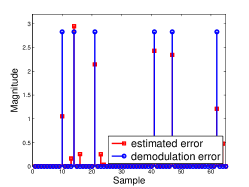
(a)

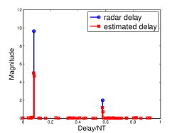
(b)

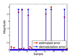
(c)

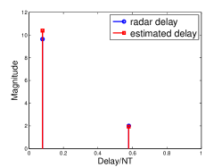
(d)

Figure 1: Comparison between (a)(b) CS-L1 algorithm and (c)(d) CS-AN algorithm.

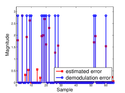
(a)

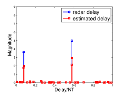
(b)

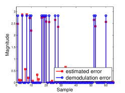
(c)

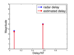
(d)

Figure 2: Comparison between (a)(b) CS-L1 algorithm and (c)(d) CS-AN algorithm.

IV Fast Algorithm Based on Non-convex Factorization

As outlined in the previous section, the off-the-shelf solvers for (III-B) tend to be slow, especially for large-dimensional cases. A possible alternative, in these circumstances, could be the Alternating Direction Method of Multipliers (ADMM) [44], which requires an eigenvalue decomposition at each iteration, still entailing a computational complexity ${\cal O}((N+K)^{3})$ per iteration, again posing a complexity issue for large-scale problems.

In this section, we derive a fast method for solving this SDP via the non-convex factorization proposed by Burer and Monteiro [45]. For notational simplicity, the superscript $l$ of the variables $\bm{z}$ and $\bm{v}$ are omitted in what follows. Defining

$$\bm{Z} = \left[{\begin{array}[]{*{20}{c}}\bm{U}&\bm{X}^{H}\\ \bm{X}&\bm{T}\end{array}}\right]\in\mathbb{C}^{(N+K)\times(N+K)},$$ (46)

we rewrite (III-B) as

$$\mathop{\min}\limits_{\bm{Z},\bm{v}} \sum_{k=-\tilde{N}_{1}}^{\tilde{N}_{2}}\frac{1}{2}{\left|z(k)-\left\langle\bm{f}_{k},\bm{H}\bm{A}\bm{v}\right\rangle-\left\langle\bm{X},\bm{\bar{d}}_{k}\bm{e}_{k}^{H}\right\rangle\right|^{2}}$$ (47)

$$+\frac{\lambda}{2N}{\text{Tr}}\left(\bm{U}\right)+\frac{\lambda\text{Tr}(\bm{T})}{2}+\gamma\|\bm{v}\|_{1},$$

s.t. $${\cal P}_{\rm Toep}(\bm{U})=\bm{U},\bm{Z}\succeq 0,$$

where ${\cal P}_{\rm Toep}(\cdot)$ denotes the projection of the input matrix onto a Toeplitz matrix. In particular, we have

$${\cal P}_{\text{Toep}}(\bm{U}) = \text{Toep}({\cal G}(\bm{U}))$$ (48)

with ${\cal G}(\bm{U})$ outputing an $N$-dimensional vector whose $(k+1)$-th element is the mean value of the $k$-th subdiagnal elements of the input matrix, i.e., ${\cal G}(\bm{U})_{k+1}=\frac{1}{N-k}\sum_{j=1}^{N-k}U(k+j,j)$.

As will be shown later, the algorithm can be accelerated if the solution to (47) is of low-rank. Note that the number of active radars is usually small in practice, which leads to small $\hat{J}$. We show in the following lemma that under some conditions the rank of the solution for $\bm{Z}$ equals $\hat{J}$, which enables us to accelerate the algorithm through non-convex factorization. The proof is given in Appendix B.

Lemma 2

Suppose $\bm{\hat{X}}=\sum_{j=1}^{\hat{J}}\hat{c}_{j}\bm{\hat{h}}_{j}\bm{a}(\hat{\tau}_{j}^{\prime})^{H}$ is the solution to (III-B). If $N\geq 257$ and $\Delta_{\hat{\tau}^{\prime}}\geq\frac{4}{N-1}$ where

$$\Delta_{\hat{\tau}^{\prime}}=\inf_{\hat{\tau}_{1}^{\prime},\hat{\tau}_{2}^{\prime}\in[0,1]:\hat{\tau}_{1}^{\prime}\neq\hat{\tau}_{2}^{\prime}}\min\left\{|\hat{\tau}_{1}^{\prime}-\hat{\tau}_{2}^{\prime}|,1-|\hat{\tau}_{1}^{\prime}-\hat{\tau}_{2}^{\prime}|\right\},$$ (49)

then there exists $\bm{\hat{Z}}$ as a solution to (47) that satisfies $\text{rank}(\bm{\hat{Z}})=\hat{J}$.

If an upper bound on the number of active radars, say $\bar{J}$, is known in advance, then we can introduce the extra constraint $\text{rank}(\bm{Z})\leq\bar{J}$ in (47), whereby restricting the search space to matrices of rank at most $\bar{J}$ does not change the globally optimal value. Additionally, we relax the constraint ${\cal P}_{\rm Toep}(\bm{U})=\bm{U}$, replacing it with the penalty term $\frac{\varrho}{2}\|{\cal P}_{\rm Toep}(\bm{U})-\bm{U}\|_{F}^{2}$, so that the problem is recast as

$$\mathop{\min}\limits_{\bm{Z},\bm{v}} \zeta(\bm{Z},\bm{v})=\frac{\lambda}{2N}{\text{Tr}}\left(\bm{U}\right)$$ (50)

$$+\sum_{k=-\tilde{N}_{1}}^{\tilde{N}_{2}}\frac{1}{2}{\left|z(k)-\left\langle\bm{f}_{k},\bm{H}\bm{A}\bm{v}\right\rangle-\left\langle\bm{X},\bm{\bar{d}}_{k}\bm{e}_{k}^{H}\right\rangle\right|^{2}}$$

$$+\frac{\lambda\text{Tr}(\bm{T})}{2}+\frac{\varrho}{2}\|{\cal P}_{\rm Toep}(\bm{U})-\bm{U}\|_{F}^{2}+\gamma\|\bm{v}\|_{1},$$

s.t. $$\bm{Z}\succeq 0,\text{rank}(\bm{Z})\leq\bar{J}.$$

Setting $\bm{Z}=\bm{V}\bm{V}^{H}$ where $\bm{V}\in\mathbb{C}^{(N+K)\times\bar{J}}$, (50) becomes an unconstrained optimization of $\min_{\bm{V},\bm{v}}\zeta(\bm{V}\bm{V}^{H},\bm{v})$. Though this unconstrained problem is non-convex, its dimension is lower than that of the original problem in (47) and has no conic constraint, which leads to reduced computational complexity. A very effective means to undertake the desired minimization of $\zeta(\bm{V}\bm{V}^{H},\bm{v})$ is to resort to a Conjugate Gradient (CG) algorithm [46], which is a fast first-order algorithm. The algorithm requires the objective function to be smooth, therefore we approximate $\|\cdot\|_{1}$ in $\zeta(\bm{V}\bm{V}^{H},\bm{v})$ with the convex, differentiable function:

$$\|\bm{v}\|_{1} \approx \psi_{\mu}(\bm{v})$$ (51)

$$= \mu\sum_{m=0}^{M-1}\log\left(\frac{\exp(|v_{m}|/\mu)+\exp(-|v_{m}|/\mu)}{2}\right)$$

$$= \mu\sum_{m=0}^{M-1}\log\cosh(|v_{m}|/\mu)$$

where $\mu$ controls the smoothing level . Hence, the problem becomes

$$\mathop{\min}\limits_{\bm{V},\bm{v}} \tilde{\zeta}(\bm{V}\bm{V}^{H},\bm{v}),$$ (52)

where

$$\tilde{\zeta}(\bm{Z},\bm{v}) = \sum_{k=-\tilde{N}_{1}}^{\tilde{N}_{2}}\frac{1}{2}{\left|z(k)-\left\langle\bm{f}_{k},\bm{H}\bm{A}\bm{v}\right\rangle-\left\langle\bm{X},\bm{d}_{k}\bm{e}_{k}^{H}\right\rangle\right|^{2}}$$ (53)

$$+\frac{\lambda}{2N}{\text{Tr}}\left(\bm{U}\right)+\frac{\lambda\text{Tr}(\bm{T})}{2}$$

$$+\frac{\varrho}{2}\|{\cal P}_{\rm Toep}(\bm{U})-\bm{U}\|_{F}^{2}+\gamma\psi_{\mu}(\bm{v}).$$

The minimization problem (52) can be effectively solved using the CG algorithm, undertaking the iteration

$$\bm{V}^{(k)} = \bm{V}^{(k-1)}+\varsigma_{k}\bm{P}_{k},$$ (54)

$$\bm{v}^{(k)} = \bm{v}^{(k-1)}+\varsigma_{k}\bm{p}_{k},$$ (55)

where $\varsigma_{k}$ is the step size, $\bm{p}_{k}$ and $\bm{P}_{k}$ are the search directions at step $k$, evaluated as the weighted sums of the gradients at present iteration and the search direction used at the previous one. Specifically, if $\nabla_{\bm{V}}\tilde{\zeta}(\bm{V}^{(k-1)}(\bm{V}^{(k-1)})^{H},\bm{v}^{(k-1)})$ and $\nabla_{\bm{v}}\tilde{\zeta}(\bm{V}^{(k-1)}(\bm{V}^{(k-1)})^{H},\bm{v}^{(k-1)})$ denote the gradients of $\tilde{\zeta}(\bm{V}\bm{V}^{H},\bm{v})$ at the $k$-th iteration, then we have

$$\bm{P}_{k} = -\nabla_{\bm{V}}\tilde{\zeta}(\bm{V}^{(k-1)}(\bm{V}^{(k-1)})^{H},\bm{v}^{(k-1)})+\omega_{k}\bm{P}_{k-1},$$ (56)

$$\bm{p}_{k} = -\nabla_{\bm{v}}\tilde{\zeta}(\bm{V}^{(k-1)}(\bm{V}^{(k-1)})^{H},\bm{v}^{(k-1)})+\omega_{k}\bm{p}_{k-1},$$ (57)

where

$$\omega_{k}=\frac{\left[\begin{array}[]{l}\left\langle\nabla_{\bm{V}}\tilde{\zeta}(\bm{V}^{(k-1)}(\bm{V}^{(k-1)})^{H},\bm{v}^{(k-1)}),\bm{Q}_{k-1}\right\rangle\\ +\left\langle\nabla_{\bm{v}}\tilde{\zeta}(\bm{V}^{(k-1)}(\bm{V}^{(k-1)})^{H},\bm{v}^{(k-1)}),\bm{q}_{k-1}\right\rangle\end{array}\right]}{\left\langle\bm{P}_{k-1},\bm{Q}_{k-1}\right\rangle+\left\langle\bm{p}_{k-1},\bm{q}_{k-1}\right\rangle},$$ (60)

with $\bm{Q}_{k}=\nabla_{\bm{V}}\tilde{\zeta}(\bm{V}^{(k)}(\bm{V}^{(k)})^{H},\bm{v}^{(k)})-\nabla_{\bm{V}}\tilde{\zeta}(\bm{V}^{(k-1)}(\bm{V}^{(k-1)})^{H},\bm{v}^{(k-1)})$ and $\bm{q}_{k}=\nabla_{\bm{v}}\tilde{\zeta}(\bm{V}^{(k)}(\bm{V}^{(k)})^{H},\bm{v}^{(k)})-\nabla_{\bm{v}}\tilde{\zeta}(\bm{V}^{(k-1)}(\bm{V}^{(k-1)})^{H},\bm{v}^{(k-1)})$. The expressions of the gradients are derived in Appendix C.

For clarity, we summarize the proposed non-convex solver in Algorithm 2. To guarantee that the objective function does not increase with $k$, the CG utilizes the Armijo line search [48] (line 6 of Algorithm 2), so that the algorithm converges to a stationary point of the surrogate problem, namely, the point where the smoothed objective function (53) has vanishing gradient.

Algorithm 2 Conjugate gradient algorithm

Input $\bar{\bm{D}}$, $\bm{z}$, $N$, $\lambda$, $\gamma$, $\epsilon$, $\varrho$, $\mu$.

1, Initialize $\bm{V}^{(0)}$, $\bm{v}^{(0)}$, $k=0$.

Do

2,     $k=k+1$.

3,     Compute $\nabla_{\bm{V}}\tilde{\zeta}(\bm{V}^{(k-1)}(\bm{V}^{(k-1)})^{H},\bm{v}^{(k-1)})$ and

$\nabla_{\bm{v}}\tilde{\zeta}(\bm{V}^{(k-1)}(\bm{V}^{(k-1)})^{H},\bm{v}^{(k-1)})$.

If $k=1$

4,        $\bm{P}_{k}=-\nabla_{\bm{V}}\tilde{\zeta}(\bm{V}^{(k-1)}(\bm{V}^{(k-1)})^{H},\bm{v}^{(k-1)})$,

$\bm{p}_{k}=-\nabla_{\bm{v}}\tilde{\zeta}(\bm{V}^{(k-1)}(\bm{V}^{(k-1)})^{H},\bm{v}^{(k-1)})$,

Else

5,        Calculate $\bm{P}_{k}$ and $\bm{p}_{k}$ according to (56) and

(57) where $\omega_{k}$ is obtained by (60).

End if

6,     Update $\bm{V}^{(k)}$ and $\bm{v}^{(k)}$ according to (54) and (55)

where $\varsigma_{k}$ is obtained via Armijo line search.

While $\|\nabla_{\bm{V}}\tilde{\zeta}(\bm{V}^{(k)}(\bm{V}^{(k)})^{H})\|_{2}\leq\epsilon$.

7, Obtain $\bm{\hat{X}}$ according to (46) with $\bm{\hat{Z}}=\bm{V}^{(k)}(\bm{V}^{(k)})^{H}$.

Return $\bm{\hat{v}}=\bm{v}^{(k)}$, $\bm{\hat{X}}$.

The computational complexity of the proposed algorithm at each iteration is mainly determined by the calculation of $\bm{V}\bm{V}^{H}$, whose complexity is ${\cal O}((N+K)^{2}\bar{J})$. As $\bar{J}$ is much smaller than $(N+K)$, the complexity per-iteration is much smaller than that of a classical eigenvalue decomposition, whereby, for large-dimensional problems, the proposed non-convex approach can be faster than those based on the first-order methods such as ADMM and projected gradient descent. We illustrate this fact through a simulation example, whose results are reported in Fig. 3. The dimension of the signal is $N=257$, while the other parameters are $J=2$, $L=5$ and $K=5$. The variance of the noise is $\sigma_{w}^{2}=0.01$. The non-convex solver is implemented by solving (52) with the CG algorithm. We compare the MSE of the proposed algorithm with that given by solving (III-B) with CVX [49] and ADMM solver. As can be seen from Fig. 3, the result of the proposed algorithm is close to the solution given by the CVX after 1000 iterations: since the proposed algorithm is also much faster than the ADMM, it appears much more suitable for real-time implementation.

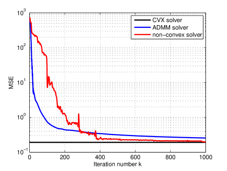
Figure 3: Convergence behavior of the proposed non-convex solver. The non-convex solver takes 41.2 seconds with 1000 iterations. The ADMM solver takes 104.2 seconds with 1000 iterations. The CVX solver takes 228.7 seconds. The experiments were carried out on an Intel Xeon desktop computer with a 3.5 GHz CPU and 24 GB of RAM.

V Simulation Results

V-A Simulation Setup

In order to demonstrate the performance of the proposed algorithms, we simulate a scenario with multiple radars and one communication receiver. The communication system uses OFDM signal with frequency spacing between adjacent subcarrier of 10kHz, $N=129$ subcarrier frequencies and total bandwidth 1.29MHz. The symbol length is $T=100\mu s$ and Quadrature Phase-Shift Keying (QPSK) modulation is used. The channel matrix is generated as $\bm{F}^{H}\bm{\Gamma}\bm{F}$ where $\bm{\Gamma}$ is an identity matrix whose diagonal elements are complex random variables whose moduli follow a Ricean distribution: as a consequence, we model the ray impinging on the receiver as the superposition of a non-fading component, with power $\rho^{2}$ say, and a fluctuating (zero-mean) component, with mean square value $\sigma^{2}_{h}$, so that the Rician factor is $\frac{\rho^{2}}{\sigma^{2}_{h}}$ [50, p. 79]. As to the active radars, they are modeled as point sources in our simulations. For simplicity, the amplitudes of the path gains $c_{j}$ are generated with fixed magnitude and random phase, and the magnitude is controlled by the power of the paths. We define the signal-to-interference ratio (SIR) at the communication RX as the power ratio of the communication signal and the radar interference. Specifically, the SNR and SIR are defined as

SNR $$= \frac{(\rho^{2}+\sigma_{h}^{2})\varepsilon_{b}}{\sigma_{w}^{2}},$$ (61)

SIR $$= \frac{N\varepsilon_{b}(\rho^{2}+\sigma_{h}^{2})}{\left\|\sum_{j=1}^{J}c_{j}\bm{g}_{j}\right\|_{2}^{2}},$$ (62)

where $\varepsilon_{b}$ is the average energy of the signal constellation. Notice that, for fixed SNR, lower values of $\rho$ account for larger fluctuations, up to the limit $\rho=0$, $\text{SNR}=\frac{\sigma_{h}^{2}\varepsilon_{b}}{\sigma_{w}^{2}}$, which corresponds to a Rayleigh-fading channel. In what follows we use $\frac{\rho}{\sigma_{h}}=3$, unless otherwise specified and then study the impact of the channel fluctuation on the achievable performance.

In keeping with the model of Section II, $\bm{\bar{g}}_{j}$ lives in a low-dimensional subspace spanned by the columns of $\bar{\bm{D}}$ matrix, i.e., $\bm{\bar{g}}_{j}=\bar{\bm{D}}\bm{h}_{j}$. We use the setting that $\bar{\bm{D}}=\bm{F}\bm{D}$ where $\bm{D}=[\bm{d}_{1},\bm{d}_{2},...,\bm{d}_{K}]\in\mathbb{C}^{N\times K}$ with $\bm{d}_{k}\in\mathbb{C}^{N\times 1}$ and $K=5$. In our simulation, the radars use pulse waveforms and each pulse uses Gaussian random code with length $N^{\prime}=32$. Specifically, $\bm{d}_{k}$ satisfies $d_{k}(m)\sim{\cal CN}(0,1/N^{\prime})$ for $1\leq m\leq N^{\prime}$ and $d_{k}(m)=0$ for $N^{\prime}+1\leq m\leq N$. The columns of $\bar{\bm{D}}$ can be obtained by taking the DFT of $\bm{d}_{k}$. Fig. 4 gives an example of the signal at the communication RX when $J=1$. The SIR of the example is set as 0dB: The figure clearly demonstrates how dramatic the effect of even a single co-existing radar can be.

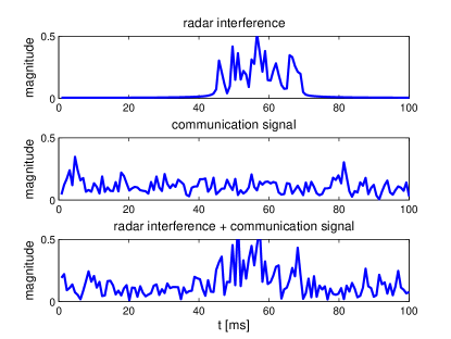
(a)

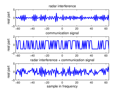
(b)

Figure 4: Plots of radar interfernce, communication signal and the received signal of communication RX in (a) time domain and (b) frequency domain. In (a), the magnitude of the signal is plotted against time. In (b), the real part of the signal is plotted versus frequency sample.

Some other parameters of the simulations are given as follows.

1, The $\tau_{j}$’s are randomly generated between $10\mu s$ and $70\mu s$ for $j=1,2,...,J$.

2, For comparison purposes, we also show the performance of $\bm{\hat{b}}=\Psi(\bm{\bar{r}})$, i.e. of a demodulator operating on the raw data: this is named “Iteration 0”, since its result is the initial point to be provided to the iterative algorithms.

3, For the proposed CS-L1 algorithm, we discretize the continuous parameter space to a finite set of grid points of cardinality $\tilde{J}=4N$. The weights for CS-L1 are $\tilde{\lambda}=\sigma_{w}\kappa\sqrt{2\log(\tilde{J}K)}$ and $\tilde{\gamma}=0.5\sigma_{w}\sqrt{2\log(\tilde{J}K)}$, where $\kappa$ is the average norm of the column vectors of matrix $\bm{\Upsilon}$.

4, For the proposed CS-AN algorithm, the weights are set as $\lambda=\sigma_{w}\sqrt{KN\log(KN)}$ and $\gamma=\frac{\lambda}{\sqrt{N}}$. We use the proposed non-convex algorithm to solve (52) where $\bar{J}=10$, $\mu=0.01$ and $\varrho=5$. The algorithm stops as the norm of the gradient is smaller than 0.01.

5, We evaluate the root-mean-squared-error (RMSE) of the radar delay estimation and the relative mean-squared-error (MSE) of the estimated waveform for the proposed CS-L1 and CS-AN algorithms. Notice that the algorithms return a bunch of $\hat{\tau}_{j}$’s, which can be either true detections or false alarms, and a radar cannot be identified if there is no $\hat{\tau}_{j}$ close to its position. We thus refer to the RMSE conditioned on correct radars identification: in undertaking simulation, a radar is declared to be correctly identified if there is a $\hat{\tau}_{j}$ whose error is smaller than $T/4$, which is the grid sizes of the simulated CS-L1 algorithm. Specifically, the delay RMSE and relative waveform MSE are calculated as

$$\text{RMSE}_{\tau} = \sqrt{\frac{1}{\text{MC}}\sum_{m=1}^{\text{MC}}\frac{1}{|\Omega_{m}|}\sum_{j\in\Omega_{m}}(\tau_{j}^{(m)}-\hat{\tau}_{j}^{(m)})^{2}},$$ (63)

$$\text{MSE}_{cg} = \frac{1}{\text{MC}}\sum_{m=1}^{\text{MC}}\frac{1}{|\Omega_{m}|}\sum_{j\in\Omega_{m}}\frac{\left\|c_{j}^{(m)}\bm{g}_{j}^{(m)}-\hat{c}_{j}^{(m)}\bm{\hat{g}}_{j}^{(m)}\right\|_{2}^{2}}{\left\|c_{j}^{(m)}\bm{g}_{j}^{(m)}\right\|_{2}^{2}},$$

respectively, where MC is the number of runs; $\Omega_{m}$ is the index set of the identified radars in the $m$-th simulation; $|\cdot|$ denotes the cardinality of the input set; $\tau_{j}^{(m)}$, $c_{j}^{(m)}$ and $\bm{g}_{j}^{(m)}$ are the delay, path gain and waveform of the $j$-th radar in the $m$-th run, respectively, while $\hat{\tau}_{j}^{(m)}$ and $\hat{c}_{j}^{(m)}\bm{\hat{g}}_{j}^{(m)}$ are the respective estimates.

V-B Performance

We compare the SER performance of the proposed algorithms. The number of active radars is set as $J=2$ in the simulation. We firstly analyze the impact of iterations on the performance of the proposed CS-L1 and CS-AN algorithms. In Fig. 5, the SER of the algorithms are plotted against the iteration number. As can be seen from the figure, both the CS-L1 and the CS-AN algorithms converge monotonically, but CS-AN converges to a much smaller demodulation error. The algorithms usually converge within 10 iterations.

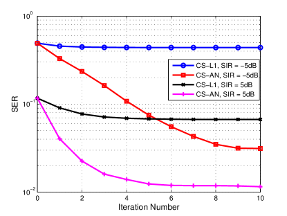
(a)

Figure 5: Plots of SER against the iteration number. The SNR is set as 15dB in the simulations.

In Fig. 6, the effect of the SNR is studied: both proposed CS-L1 and CS-AN algorithms provide better SER performance than Iteration 0. The CS-AN algorithm also outperforms the CS-L1 algorithm in all situations. In order to quantify the cost incurred by the lack of cooperation between the active radars and the communication system, we also report the performance of the algorithm assuming known radar delays, i.e. of the modified CS-L1 algorithm presented in Section III-A: in undertaking the simulation, we set $\tilde{\gamma}=2\sigma_{w}\sqrt{2\log(N)}$ for such algorithm. As expected, known radar delays result in visibly better SER, which is the reward for the additional overhead due to the transmission of pilot signals and for the increased overall complexity due to system co-ordination.

Notice that, as the SNR is 8dB, the performance gain achieved by both CS algorithms is limited: this is obviously due to the fact that, under fading channel, the performance of even an interference-free OFDM/QPSK would be poor, and the coupling between data demodulation and interference removal explains the poor performance at low SIR. For example, the considered Ricean channel with Rice factor 9 is approximately equivalent to a Nakagami-m fading with parameter $m\simeq 5.3$ [50, p.79], whereby the error probability for an isolated OFDM/QPSK at $\text{SNR}=10$dB would be slightly larger than $10^{-2}$, a value which is approximately restored as the SIR becomes increasingly large.

As the SNR is larger than 14dB, the CS-L1 provides significant improvements over Iteration 0, but is significantly outperformed by the CS-AN especially when SIR is -5dB. This is due to the fact that, in the low SIR region, basis mismatch prevents correcting the demodulation errors in the first iteration $\bm{\hat{b}}^{(0)}$ through a CS-L1 algorithm, while the CS-AN algorithm, much more accurate in detecting and ranging the interference sources, allows a much more effective error correction. Needless to say, both algorithms restore the original OFDM/QPSK performance for increasingly large SIR in a much faster way than Iteration 0: it might thus be inferred that, even at SIR as low as -5dB, the SER achieved through the proposed CS-AN algorithm - in the order of $10^{-2}$ - would in principle allow communication to be sustained once forward error correction (FEC) decoding [51] is undertaken, while no communication could take place if either of the other two algorithms were adopted.

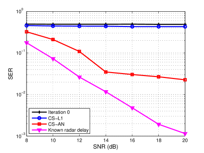
(a)

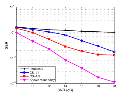
(b)

Figure 6: Comparison of the algorithm SERs when the SIR of communication is (a) -5dB and (b) 5dB.

We then evaluate the relative waveform MSE and delay RMSE of the proposed CS-L1 and CS-AN algorithms. Note that the received signal contains both communication and radar signal, and the estimation accuracy depends on both the power of the radar signals to be estimated and the performance of the demodulator: as a consequence, the estimation accuracy may be not necessarily increasing with the SIR, especially for “intermediate” SIR values where radar signals are not strong enough to prevail on the communication signal, but still produce significant demodulation error. In Fig. 7, the relative waveform MSE and delay RMSE is represented as a function of the SNR. As expected, the CS-AN algorithm provides much better accuracy than the CS-L1 algorithm. Notice also the apparently contradictory effects of the SNR. Indeed, large SNR’s guarantee good demodulation performance, with a beneficial effect on the interference estimation due to the coupling. Under this point of view, the advantage of the CS-AN over the CS-L1 is visible, and the former seems to take much greater advantage of the more reliable demodulation process granted by larger values of the SNR.

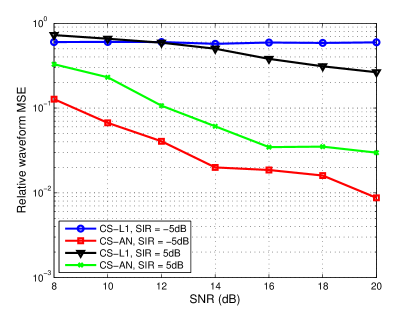
(a)

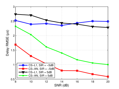
(b)

Figure 7: Plots of (a) relative waveform MSE and (b) delay RMSE for different SNRs.

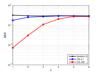
(a)

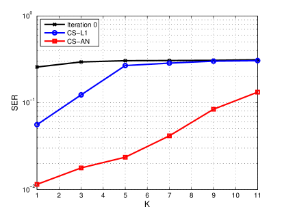
(b)

Figure 8: Plots of SER against (a) $J$, and (b) $K$.

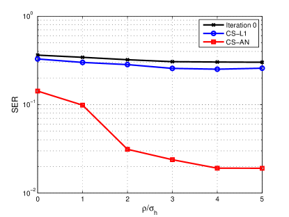
(a)

Figure 9: Plots of SER against $\rho/\sigma_{h}$.

The effects of $J$ and $K$ are elicited in Fig. 8. The simulations are run with an SNR of 18dB and an SIR of 0dB. In Fig. 8a, we set $\rho/\sigma_{h}=3$ and plot the SER against the number of active radars: As $J$ increases, the sparsity of the problem is reduced, and the sources of interference - with the respective unknown parameters to be estimated - increase, which obviously results in a visible performance degradation for both algorithms, up to a point that not even an CS-AN algorithm is effective if $J\geq 5$. In Fig. 8b, the number of active radars is set as $J=2$ and we examine the SER behavior for varying dictionary size $K$. Although a performance degradation is evident, the robustness of the CS-AN algorithm to $K$ is a definitely appealing advantage over the other two algorithms. Finally, we investigate the effect of the channel model on the performance in Fig. 9, assuming $J=2$, SIR$=0$dB and SNR$=18$dB. On the horizontal axis we represent the Ricean factor, whereby decreasing values of $\rho/\sigma_{h}$ represent weaker and weaker direct paths, up to the case $\rho=0$ where no direct path is present. Notice that only the CS-AN algorithm guarantees, in such a severe scenario, an acceptable performance and is able to restore an error probability in the order of $10^{-2}$ as $\rho/\sigma_{h}>2$.

VI Conclusions

In this paper, we have proposed two algorithms for joint waveform estimation and demodulation in the overlaid communication and radar systems. One of them is based on the on-grid compressed sensing (CS) technique and uses $\ell_{1}$-norm to exploit the sparsity of the radar signal components and the sparsity of the demodulation error. The other one is a CS-based algorithm using both the atomic norm and the $\ell_{1}$-norm to exploit the sparsity of the radar signal components and the sparsity of the demodulation error, respectively. We have derived a fast algorithm to compute the solution to the formulated CS-AN problem. Simulation results show that the proposed algorithms provide better SER compared to the original demodulation. Future work will include extending the algorithm to the fast time-varying environment in which the mismatch in communication channel estimation and radar Doppler are considered.

-A Accuracy Analysis of (10)

Some approximation has been applied to (8) before we get (10). In this section, the accuracy of our approximation is analyzed. As anticipated (9) holds rigorously if $0\leq\beta\leq 1/N$ and approximately for small to moderate excess bandwidths [36]. With small $\beta$, the approximation error comes from (8) when we extend the integration from a finite range to infinite, which causes descrepency between $\bar{r}(k)$ and the one calculated by (10). For clarity, we denote $\tilde{r}(k)$ as the approximated $\bar{r}(k)$ calculated by (10). Let $S_{\xi}(f)={\cal F}(R_{\xi}(t))$, then $R_{\xi}(t)={\cal F}^{-1}(S_{\xi}(f))$, where ${\cal F}(\cdot)$ and ${\cal F}^{-1}(\cdot)$ denote the Fourier transform and inverse Fourier transform, respectively. We have

$$R_{\xi}(t)\sim\frac{1}{t^{m+1}},t\to+\infty,$$ (65)

where $m$ is the order of the first discontinuous derivative of $S_{\xi}(f)$. In our paper, $\xi(\cdot)$ is a SRRC with small roll-off factor $\beta$. So $S_{\xi}(f)$ is not only continuous - as all correlations - but also differentiable - whereby $m>1$ in (65). In fact in our setup the correlation goes to zero as $t^{-3}$. Suppose for $t\geq\bar{T}$ we have ${R_{\xi}}(t)\leq\frac{1}{\bar{T}^{m_{0}+1}}$ with $\bar{T}=T^{\prime}-\tau_{\min}$ and $m_{0}>1$. Then the approximation error can be bounded as (-A)

$$\left|{\bar{r}(k)-\tilde{r}(k)}\right| \leq \left|{\sum\limits_{n=0}^{N-1}{x(n)\left(\begin{array}[]{l}\int_{{\tau_{\min}}-nT-T^{\prime}}^{{\tau_{\max}}+(N-n-1)T+T^{\prime}}{{R_{\xi}}(t){e^{-\frac{{i2\pi k(t+nT)}}{{NT}}}}dt}\\ -\int_{-\infty}^{\infty}{{R_{\xi}}(t){e^{-\frac{{i2\pi k(t+nT)}}{{NT}}}}dt}\end{array}\right)}}\right|$$

$$+\left|{\sum\limits_{j=1}^{J}{\sum\limits_{n=0}^{N-1}{{c_{j}}{g_{j}}(n)\left(\begin{array}[]{l}\int_{{\tau_{\min}}-nT-T^{\prime}-{\tau_{j}}}^{{\tau_{\max}}+(N-n-1)T+T^{\prime}-{\tau_{j}}}{{R_{\xi}}(t){e^{-\frac{{i2\pi k(t+nT+{\tau_{j}})}}{{NT}}}}dt}\\ -\int_{-\infty}^{\infty}{{R_{\xi}}(t){e^{-\frac{{i2\pi k(t+nT+{\tau_{j}})}}{{NT}}}}dt}\end{array}\right)}}}\right|$$

$$\leq \sum\limits_{n=0}^{N-1}{\left|{2x(n)}\right|\int_{\bar{T}}^{\infty}{\left|{{R_{\xi}}(t){e^{-\frac{{i2\pi k(t+nT)}}{{NT}}}}}\right|dt}}$$

$$+\sum\limits_{j=1}^{J}{\sum\limits_{n=0}^{N-1}{\left|{2{c_{j}}{g_{j}}(n)}\right|\int_{{{\bar{T}}}}^{\infty}{\left|{{R_{\xi}}(t){e^{-\frac{{i2\pi k(t+nT+{\tau_{j}})}}{{NT}}}}}\right|dt}}}$$

$$\leq \sum\limits_{n=0}^{N-1}{\left|{2x(n)}\right|\int_{\bar{T}}^{\infty}{{t^{-{m_{0}}-1}}dt}}+\sum\limits_{j=1}^{J}{\sum\limits_{n=0}^{N-1}{\left|{2{c_{j}}{g_{j}}(n)}\right|\int_{{{\bar{T}}}}^{\infty}{{t^{-{m_{0}}-1}}dt}}}$$

$$\leq \sum\limits_{n=0}^{N-1}{\frac{{2\left|{x(n)}\right|}}{{{m_{0}}{{\bar{T}}^{{m_{0}}}}}}}+\sum\limits_{j=1}^{J}{\sum\limits_{n=0}^{N-1}{\frac{{2\left|{{c_{j}}{g_{j}}(n)}\right|}}{{{m_{0}}{{\bar{T}}^{{m_{0}}}}}}}},$$ (72)

where the second inequality is the result of relation

$$\bar{T}\leq\min_{1\leq j\leq J,0\leq n\leq N-1}\left\{\begin{array}[]{l}{\tau_{\max}}-{\tau_{j}}+(N-n-1)T+T^{\prime},\\ T^{\prime}+nT-{\tau_{\min}}\end{array}\right\}.$$

Obviously, as $T^{\prime}$ is very large, $\bar{T}$ becomes large so the approximation error is very small.

-B Proof of Lemma 2

Suppose the solution to (III-B) is $\bm{\hat{X}}=\sum_{j=1}^{\hat{J}}\hat{c}_{j}\bm{\hat{h}}_{j}\bm{a}(\hat{\tau}_{j}^{\prime})^{H}$, the following lemma states the condition of the unique atomic decomposition:

Lemma 3

[24] $\bm{\hat{X}}$ is the unique atomic decomposition satisfying that $\|\bm{\hat{X}}\|_{\cal A}=\sum_{j=1}^{\hat{J}}|\hat{c}_{j}|$ if $N\geq 257$ and $\Delta_{\hat{\tau}^{\prime}}\geq\frac{1}{(N-1)/4}$.

The lemma above gives the value of $\|\bm{\hat{X}}\|_{\cal A}$. Since (III-B) and (47) are equivalent, we obtain

$$\|\bm{\hat{X}}\|_{\cal A}=\mathop{\inf}\limits_{\bm{\hat{U}},\bm{\hat{T}}}\left\{\begin{array}[]{l}\frac{1}{2N}{\rm{Tr}}(\bm{\hat{U}})+\frac{1}{2}{\rm Tr}(\bm{\hat{T}}),\\ {\rm s.t.,}{\cal P}_{\rm Toep}(\bm{\hat{U}})=\bm{\hat{U}},\bm{\hat{Z}}\succeq 0\end{array}\right\},$$ (75)

where the relation of $\bm{\hat{Z}}$, $\bm{\hat{U}}$ and $\bm{\hat{T}}$ are given in (46). Hence, $\bm{\hat{Z}}$ is the solution to (47) once the equality holds. Then we need to prove that there exist Toeplitz matrix $\bm{\hat{U}}$ and matrix $\bm{\hat{T}}$ such that $\frac{1}{2N}{\text{Tr}}\left(\bm{\hat{U}}\right)+\frac{\text{Tr}(\bm{\hat{T}})}{2}=\|\bm{\hat{X}}\|_{\cal A}$ with $\text{rank}(\bm{\hat{Z}})=\hat{J}$ and ${\bm{\hat{Z}}}\succeq 0$. Let $\bm{\hat{u}}=\sum_{j=1}^{\hat{J}}\hat{c}_{j}\bm{a}(\hat{\tau}_{j}^{\prime})^{H}$. Following the Caratheodory-Toeplitz lemma [52, 28], we have

$$\bm{\hat{U}}=\text{Toep}(\bm{\hat{u}})=\sum_{j=1}^{\hat{J}}|\hat{c}_{j}|\bm{a}(\hat{\tau}_{j}^{\prime})\bm{a}(\hat{\tau}_{j}^{\prime})^{H}.$$ (76)

In such case, the matrix

$$\bm{\hat{Z}}=\sum_{j=1}^{\hat{J}}|\hat{c}_{j}|\left[{\begin{array}[]{*{20}{c}}e^{i\hat{\varphi}_{j}}\bm{a}(\hat{\tau}_{j}^{\prime})\\ \bm{\hat{h}}_{j}\end{array}}\right]\left[{\begin{array}[]{*{20}{c}}e^{-i\hat{\varphi}_{j}}\bm{a}(\hat{\tau}_{j}^{\prime})^{H}&\bm{\hat{h}}_{j}^{H}\end{array}}\right]\succeq 0$$ (80)

is rank-$\hat{J}$, where $\hat{\varphi}_{j}$ is the phase of $\hat{c}_{j}$. Note that $\frac{1}{2N}{\text{Tr}}\left(\bm{\hat{U}}\right)+\frac{\text{Tr}(\bm{\hat{T}})}{2}=\sum_{j=1}^{\hat{J}}|\hat{c}_{j}|=\|\bm{\hat{X}}\|_{\cal A}$, $\bm{\hat{Z}}$ is the solution to (47), which accomplishes the proof.

-C The calculation of $\nabla_{\bm{v}}\tilde{\zeta}(\bm{V}\bm{V}^{H},\bm{v})$ and $\nabla_{\bm{V}}\tilde{\zeta}(\bm{V}\bm{V}^{H},\bm{v})$

The gradient $\nabla_{\bm{v}}\tilde{\zeta}(\bm{V}\bm{V}^{H},\bm{v})$ can be directly calculated as

$$\nabla_{\bm{v}}\tilde{\zeta}(\bm{V}\bm{V}^{H},\bm{v})=\gamma\nabla_{\bm{v}}\psi_{\mu}(\bm{v})$$

$$\sum_{k=-\tilde{N}_{1}}^{\tilde{N}_{2}}{\left(\left\langle\bm{f}_{k},\bm{H}\bm{A}\bm{v}\right\rangle+\left\langle\bm{X},\bm{\bar{d}}_{k}\bm{e}_{k}^{H}\right\rangle-z(k)\right)\bm{A}^{H}\bm{H}^{H}\bm{f}_{k}},$$

where the $m$-th element of $\nabla_{\bm{v}}\psi_{\mu}(\bm{v})\in\mathbb{C}^{M\times 1}$ is

$$\nabla_{v_{m}}\psi_{\mu}(\bm{v})=\frac{\sinh(|v_{m}|/\mu)}{\cosh(|v_{m}|/\mu)}\frac{v_{m}}{|v_{m}|}.$$ (82)

Then we derive the gradient with respect to $\bm{V}$. Following the chain rule, we have

$$\nabla_{\bm{V}}\tilde{\zeta}(\bm{V}\bm{V}^{H},\bm{v})=\left[\nabla_{\bm{Z}}\tilde{\zeta}(\bm{Z},\bm{v})|_{\bm{Z}=\bm{V}\bm{V}^{H}}\right]\bm{V},$$ (83)

and (84), so the problem becomes calculating the gradient $\nabla_{\bm{Z}}\tilde{\zeta}(\bm{Z},\bm{v})$. For the convenience of our calculation, $\tilde{\zeta}(\bm{Z},\bm{v})$ is rewritten as

$$\tilde{\zeta}(\bm{Z},\bm{v}) = \frac{\lambda\text{Tr}(\bm{U})}{2N}+\frac{\lambda\text{Tr}(\bm{T})}{2}+\sum_{k=-\tilde{N}_{1}}^{\tilde{N}_{2}}\frac{1}{2}{\left|z(k)-\left\langle\bm{f}_{k},\bm{H}\bm{A}\bm{v}\right\rangle-\left\langle\bm{X},\bm{\bar{d}}_{k}\bm{e}_{k}^{H}\right\rangle\right|^{2}}+\gamma\psi_{\mu}(\bm{v})$$ (84)

$$+\frac{\rho}{2}\left[{\sum\limits_{k=1-N}^{N-1}{\left({\underbrace{\bm{m}_{k}^{H}{\bm{m}_{k}}-\frac{1}{{N-|k|}}\bm{m}_{k}^{H}{\bm{I}_{N-|k|}}{{\bm{I}_{N-|k|}^{H}}}\bm{m}_{k}}_{\phi_{k}(\bm{m}_{k})}}\right)}}\right],$$

where $\bm{U}$, $\bm{X}$, $\bm{T}$ are submatrices of $\bm{Z}$ whose structure is given in (46), $\bm{m}_{k}\in\mathbb{C}^{(N-|k|)\times 1}$ is the $k$-th subdiagnal elements of $\bm{U}$, $\bm{I}_{k}=[1,1,...,1]^{T}$ is an $k$ dimensional all one vector. After manipulation, $\tilde{\zeta}(\bm{Z},\bm{v})$ can be rewritten in a quadratic form:

$$\tilde{\zeta}(\bm{Z},\bm{v})=\langle\bm{Z},{\cal Q}(\bm{Z})\rangle/2+\langle\bm{C},\bm{Z}\rangle+\bar{\zeta}(\bm{v}),$$ (85)

where $\bar{\zeta}(\bm{v})$ is a function that depends on $\bm{v}$; $\bm{C}$ and ${\cal Q}(\bm{Z})$ can be respectively computed by

$$\bm{C} = \frac{1}{2}\left[{\begin{array}[]{*{20}{c}}{\frac{\lambda}{N}\bm{E}}_{N}&{-\bm{\bar{Y}}^{H}}\\ {-{\bm{\bar{Y}}}}&\lambda\bm{E}_{K}\end{array}}\right],$$ (88)

and (91).

$${\cal Q}(\bm{Z}) = \left[{\begin{array}[]{*{20}{c}}{\bm{\Xi}(\bm{U})}&{\sum_{k=-\tilde{N}_{1}}^{\tilde{N}_{2}}\langle\bm{e}_{k}^{H}\bm{\bar{d}}_{k},\bm{X}^{H}\rangle\bm{e}_{k}\bm{\bar{d}}_{k}^{H}}\\ {\sum_{k=-\tilde{N}_{1}}^{\tilde{N}_{2}}\langle\bm{\bar{d}}_{k}\bm{e}_{k}^{H},\bm{X}\rangle\bm{\bar{d}}_{k}\bm{e}_{k}^{H}}&\bm{0}_{K,K}\end{array}}\right].$$ (91)

Here $\bm{0}_{K,K}\in\mathbb{C}^{K\times K}$ is a zero matrix; $\bm{E}_{N}$ is an identity matrix with dimension $N$;

$$\bm{\bar{Y}} = \sum_{k=-\tilde{N}_{1}}^{\tilde{N}_{2}}\bm{e}_{k}\bm{\bar{d}}_{k}^{H}{\left(z(k)-\left\langle\bm{f}_{k},\bm{H}\bm{A}\bm{v}\right\rangle\right)},$$ (92)

$$\bm{\Xi}(\bm{\bar{Z}}) = \frac{\rho}{2}\sum_{k=1-N}^{N-1}\text{diag}\left(\nabla{\phi}_{k}(\bm{m}_{k}),k\right),$$ (93)

with

$$\nabla{\phi}_{k}(\bm{m}_{k})=2\left({\bm{m}_{k}-\frac{1}{{N-|k|}}{\bm{I}_{N-|k|}}{{\bm{I}_{N-|k|}^{H}}}{\bm{m}_{k}}}\right),$$ (94)

and $\text{diag}(\bm{m},k)$ outputs an $N\times N$ matrix whose $k$-th sub-diagnal is the input vector $\bm{m}$, and the rest of the elements are zero. The derivative of $\tilde{\zeta}(\bm{Z},\bm{v})$ is

$$\nabla_{\bm{Z}}\tilde{\zeta}(\bm{Z},\bm{v})={\cal Q}(\bm{Z})+\bm{C}.$$ (95)

Plugging (95) into (84), $\nabla_{\bm{V}}\tilde{\zeta}(\bm{V}\bm{V}^{H},\bm{v})$ can be obtained.

References

- [1] A. R. Chiriyath, B. Paul, G. M. Jacyna, and D. W. Bliss, “Inner bounds on performance of radar and communications co-existence,” IEEE Transactions on Signal Processing, vol. 64, no. 2, pp. 464–474, 2016.
- [2] H. Griffiths and S. Blunt, “T09-Spectrum engineering and waveform diversity,” in Radar Conference. IEEE, 2014, pp. 36–36.
- [3] H. Griffiths, L. Cohen, S. Watts, E. Mokole, C. Baker, M. Wicks, and S. Blunt, “Radar spectrum engineering and management: technical and regulatory issues,” Proceedings of the IEEE, vol. 103, no. 1, pp. 85–102, 2015.
- [4] F. Hessar and S. Roy, “Spectrum sharing between a surveillance radar and secondary Wi-Fi networks,” IEEE Transactions on Aerospace and Electronic Systems, vol. 52, no. 3, pp. 1434 – 1448, 2016.
- [5] H. Deng and B. Himed, “Interference mitigation processing for spectrum-sharing between radar and wireless communications systems,” IEEE Transactions on Aerospace and Electronic Systems, vol. 49, no. 3, pp. 1911–1919, 2013.
- [6] A. Babaei, W. H. Tranter, and T. Bose, “A practical precoding approach for radar/communications spectrum sharing,” in Cognitive Radio Oriented Wireless Networks (CROWNCOM), 2013 8th International Conference on. IEEE, 2013, pp. 13–18.
- [7] A. Aubry, A. De Maio, M. Piezzo, M. M. Naghsh, M. Soltanalian, and P. Stoica, “Cognitive radar waveform design for spectral coexistence in signal-dependent interference,” in Radar Conference. IEEE, 2014, pp. 0474–0478.
- [8] A. Khawar, A. Abdel-Hadi, and T. C. Clancy, “Spectrum sharing between S-band radar and LTE cellular system: A spatial approach,” in Dynamic Spectrum Access Networks (DYSPAN), 2014 IEEE International Symposium on. IEEE, 2014, pp. 7–14.
- [9] A. Aubry, A. De Maio, M. Piezzo, and A. Farina, “Radar waveform design in a spectrally crowded environment via nonconvex quadratic optimization,” IEEE Transactions on Aerospace and Electronic Systems, vol. 50, no. 2, pp. 1138–1152, 2014.
- [10] K.-W. Huang, M. Bică, U. Mitra, and V. Koivunen, “Radar waveform design in spectrum sharing environment: Coexistence and cognition,” in Radar Conference (RadarCon), 2015 IEEE. IEEE, 2015, pp. 1698–1703.
- [11] L. Zheng, M. Lops, X. Wang, and E. Grossi, “Joint design of overlaid communication systems and pulsed radars,” IEEE Transactions on Signal Processing, vol. 66, no. 1, pp. 139–154, 2018.
- [12] S. Sodagari, A. Khawar, T. C. Clancy, and R. McGwier, “A projection based approach for radar and telecommunication systems coexistence,” in Global Communications Conference (GLOBECOM). IEEE, 2012, pp. 5010–5014.
- [13] B. Li, A. Petropulu, and W. Trappe, “Optimum co-design for spectrum sharing between matrix completion based MIMO radars and a MIMO communication system,” IEEE Transactions on Signal Processing, vol. 64, no. 17, pp. 4562–4575, 2016.
- [14] B. Li and A. Petropulu, “MIMO radar and communication spectrum sharing with clutter mitigation,” in Radar Conference (RadarConf), 2016 IEEE. IEEE, 2016, pp. 1–6.
- [15] A. Turlapaty and Y. Jin, “A joint design of transmit waveforms for radar and communications systems in coexistence,” in Radar Conference. IEEE, 2014, pp. 0315–0319.
- [16] A. Manolakos, Y. Noam, K. Dimou, and A. J. Goldsmith, “Blind null-space tracking for MIMO underlay cognitive radio networks,” in Global Communications Conference (GLOBECOM), 2012 IEEE. IEEE, 2012, pp. 1223–1229.
- [17] J. Liu, H. Li, and B. Himed, “Joint optimization of transmit and receive beamforming in active arrays,” IEEE Signal Processing Letters, vol. 21, no. 1, pp. 39–42, 2014.
- [18] L. Xiao, H. Dai, and P. Ning, “Jamming-resistant collaborative broadcast using uncoordinated frequency hopping,” IEEE Transactions on Information Forensics and Security, vol. 7, no. 1, pp. 297–309, 2012.
- [19] ——, “MAC design of uncoordinated FH-based collaborative broadcast,” IEEE Wireless Communications Letters, vol. 1, no. 3, pp. 261–264, 2012.
- [20] S. Foucart and H. Rauhut, A mathematical introduction to compressive sensing. Birkhäuser Basel, 2013, vol. 1, no. 3.
- [21] L. Stanković, I. Orović, S. Stanković, and M. Amin, “Compressive sensing based separation of nonstationary and stationary signals overlapping in time-frequency,” IEEE Transactions on Signal Processing, vol. 61, no. 18, pp. 4562–4572, 2013.
- [22] B. Jokanovic and M. Amin, “Reduced interference sparse time-frequency distributions for compressed observations,” IEEE Transactions on Signal Processing, vol. 63, no. 24, pp. 6698–6709, 2015.
- [23] C. Studer, P. Kuppinger, G. Pope, and H. Bolcskei, “Recovery of sparsely corrupted signals,” IEEE Transactions on Information Theory, vol. 58, no. 5, pp. 3115–3130, 2012.
- [24] Z. Yang and L. Xie, “Exact joint sparse frequency recovery via optimization methods,” IEEE Transactions on Signal Processing, vol. 64, no. 19, pp. 5145–5157, 2014.
- [25] Y. Chi, L. L. Scharf, A. Pezeshki, and A. R. Calderbank, “Sensitivity to basis mismatch in compressed sensing,” IEEE Transactions on Signal Processing, vol. 59, no. 5, pp. 2182–2195, 2011.
- [26] E. J. Candès and C. Fernandez-Granda, “Super-resolution from noisy data,” Journal of Fourier Analysis and Applications, vol. 19, no. 6, pp. 1229–1254, 2013.
- [27] ——, “Towards a mathematical theory of super-resolution,” Communications on Pure and Applied Mathematics, vol. 67, no. 6, pp. 906–956, 2014.
- [28] G. Tang, B. N. Bhaskar, P. Shah, and B. Recht, “Compressed sensing off the grid,” IEEE Transactions on Information Theory, vol. 59, no. 11, pp. 7465–7490, 2013.
- [29] B. N. Bhaskar, G. Tang, and B. Recht, “Atomic norm denoising with applications to line spectral estimation,” IEEE Transactions on Signal Processing, vol. 61, no. 23, pp. 5987–5999, 2013.
- [30] Z. Tan, Y. C. Eldar, and A. Nehorai, “Direction of arrival estimation using co-prime arrays: A super resolution viewpoint,” IEEE Transactions on Signal Processing, vol. 62, no. 21, pp. 5565–5576, 2014.
- [31] H. Al-Tous, I. Barhumi, and N. Al-Dhahir, “Atomic-norm for joint data recovery and narrow-band interference mitigation in ofdm systems,” in Personal, Indoor, and Mobile Radio Communications (PIMRC), 2016 IEEE 27th Annual International Symposium on. IEEE, 2016, pp. 1–5.
- [32] G. Tang, P. Shah, B. N. Bhaskar, and B. Recht, “Robust line spectral estimation,” in 2014 48th Asilomar Conference on Signals, Systems and Computers. IEEE, 2014, pp. 301–305.
- [33] A. Hassanien, M. G. Amin, Y. D. Zhang, and F. Ahmad, “Dual-function radar-communications: Information embedding using sidelobe control and waveform diversity.” IEEE Trans. Signal Processing, vol. 64, no. 8, pp. 2168–2181, 2016.
- [34] D. Guo and S. Verdú, “Randomly spread CDMA: Asymptotics via statistical physics,” IEEE Transactions on Information Theory, vol. 51, no. 6, pp. 1983–2010, 2005.
- [35] X. Zhang, J. Liu, H. Li, and B. Himed, “Maximum likelihood synchronization for dvb-t2 in unknown fading channels,” IEEE Transactions on Broadcasting, vol. 61, no. 4, pp. 615–624, 2015.
- [36] I. Glover and P. M. Grant, Digital communications. Pearson Education, 2010.
- [37] S. Boyd and L. Vandenberghe, Convex optimization. Cambridge university press, 2004.
- [38] Y. C. Eldar and M. Mishali, “Robust recovery of signals from a structured union of subspaces,” IEEE Transactions on Information Theory, vol. 55, no. 11, pp. 5302–5316, 2009.
- [39] D. Yang, G. Tang, and M. B. Wakin, “Super-resolution of complex exponentials from modulations with unknown waveforms,” IEEE Transactions on Information Theory, vol. 62, no. 10, pp. 5809–5830, 2016.
- [40] C. Fernandez-Granda, G. Tang, X. Wang, and L. Zheng, “Demixing sines and spikes: Robust spectral super-resolution in the presence of outliers,” Information and Inference: A Journal of the IMA, 2016.
- [41] Y. Chen and Y. Chi, “Robust spectral compressed sensing via structured matrix completion,” IEEE Transactions on Information Theory, vol. 60, no. 10, 2014.
- [42] A. Naha, A. K. Samanta, A. Routray, and A. K. Deb, “Determining autocorrelation matrix size and sampling frequency for MUSIC algorithm,” IEEE Signal Processing Letters, vol. 22, no. 8, pp. 1016–1020, 2015.
- [43] P. Stoica and R. L. Moses, Introduction to spectral analysis. Prentice hall Upper Saddle River, 1997, vol. 1.
- [44] S. Boyd, N. Parikh, E. Chu, B. Peleato, and J. Eckstein, “Distributed optimization and statistical learning via the alternating direction method of multipliers,” Foundations and Trends in Machine Learning, vol. 3, no. 1, pp. 1–122, 2011.
- [45] S. Burer and R. D. Monteiro, “A nonlinear programming algorithm for solving semidefinite programs via low-rank factorization,” Mathematical Programming, vol. 95, no. 2, pp. 329–357, 2003.
- [46] Y.-H. Dai and C.-X. Kou, “A nonlinear conjugate gradient algorithm with an optimal property and an improved wolfe line search,” SIAM Journal on Optimization, vol. 23, no. 1, pp. 296–320, 2013.
- [47] J. Sun, Q. Qu, and J. Wright, “Complete dictionary recovery over the sphere I: Overview and the geometric picture,” IEEE Transactions on Information Theory, vol. 63, no. 2, pp. 853–884, 2017.
- [48] N. Boumal and P.-A. Absil, “Low-rank matrix completion via preconditioned optimization on the grassmann manifold,” Linear Algebra and its Applications, vol. 475, pp. 200–239, 2015.
- [49] M. Grant and S. Boyd, “CVX: Matlab software for disciplined convex programming, version 2.1,” http://cvxr.com/cvx, Mar. 2014.
- [50] A. Godsmith, Wireless Communications. Cambridge University Press, 2005.
- [51] T. Ji and W. Stark, “Rate-adaptive transmission over correlated fading channels,” IEEE Transactions on Communications, vol. 53, no. 10, pp. 1663–1670, 2005.
- [52] C. Carathéodory, “Über den variabilitätsbereich der fourier’schen konstanten von positiven harmonischen funktionen,” Rendiconti Del Circolo Matematico di Palermo (1884-1940), vol. 32, no. 1, pp. 193–217, 1911.