Techniques for Accurate Parallax Measurements for 6.7-GHz Methanol Masers

Abstract

The BeSSeL Survey is mapping the spiral structure of the Milky Way by measuring trigonometric parallaxes of hundreds of maser sources associated with high-mass star formation. While parallax techniques for water masers at high frequency (22 GHz) have been well documented, recent observations of methanol masers at lower frequency (6.7 GHz) have revealed astrometric issues associated with signal propagation through the ionosphere that could significantly limit parallax accuracy. These problems displayed as a “parallax gradient” on the sky when measured against different background quasars. We present an analysis method in which we generate position data relative to an “artificial quasar” at the target maser position at each epoch. Fitting parallax to these data can significantly mitigate the problems and improve parallax accuracy.

1 Introduction

The Bar and Spiral Structure Legacy (BeSSeL) Survey uses the National Radio Astronomy Observatory’s Very Long Baseline Array (VLBA) to measure parallaxes of methanol and water masers associated with newly formed (or forming) high-mass stars throughout the Milky Way. In the first two years of the survey, observations were done using maser lines near 12 GHz (methanol) and 22 GHz (water). At frequencies above $\approx 10$ GHz, the dominant source of astrometric error is usually uncompensated interferometric delays associated with water vapor in the troposphere. Astrometric techniques that can yield $\sim 10$ micro-arcsec parallaxes at these frequencies are described in Honma, Tamura & Reid (2008), Reid et al. (2009) and Reid & Honma (2014).

However, only about a dozen 12-GHz methanol masers were strong enough to serve as interferometer phase-reference sources and hence be optimum targets for parallax measurements, and the BeSSeL Survey sought to use the stronger and more numerous 6.7-GHz methanol masers. Since emission line features of methanol masers are longer-lived (typically decades) than water masers (often only several months), interferometer coherence times improve with observing wavelength, and atmospheric opacity is generally lower at longer cm-wavelengths, we anticipated that parallax accuracy would be comparable to or better than those obtained at 22 GHz. So, in 2015, new wide C-band receivers, funded by the Max Planck Institute for Radio Astronomy (MPIfR), were installed on the VLBA. Unfortunately, below $\approx 10$ GHz, interferometric propagation delays associated with electrons in the ionosphere can severely increase astrometric errors, even after removing estimated ionospheric delays based on global total electron content models derived from Global Positioning System data (Walker & Chatterjee, 1999).

The BeSSeL Survey strategy has been to use the target maser as the interferometric phase-reference source and rapidly switch between the maser and background quasars, in order to remove short-term phase-delay fluctuations (mostly from water vapor) from the interferometric data. This essentially removes interferometer coherence-time limitations and allows one to use Earth rotation synthesis to improve interferometer (u,v)-coverage, imaging quality, and astrometric accuracy. We used several background quasars for each maser, to guard against occasional structural variability in a quasar limiting astrometric accuracy, as well as to provide several nearly independent parallax measurements.

Often the quasars surrounded the target maser on the sky. This was fortunate as it allowed us to detect systematic gradients in parallax estimates on the sky as sampled by the different quasars relative to the target maser source. Presumably these can be traced to uncompensated ionospheric delays that present as “wedges,” which over time-scales of hours distort relative position measurements in a quasi-linear fashion over $\mathrel{\hbox{\raise 2.15277pt\hbox{$>$}\hbox to0.0pt{\hss\lower 2.15277pt\hbox{$\sim$}}}}5^{\circ}$ on the sky. At any single epoch it would be difficult to disentangle these effects from catalog position errors, which are generally $\mathrel{\hbox{\raise 2.15277pt\hbox{$>$}\hbox to0.0pt{\hss\lower 2.15277pt\hbox{$\sim$}}}}0.1$ mas. However, for parallax measurements which involve multiple epochs spanning one year, this proved obvious as will be shown below. Since we do not see these effects at 22 GHz, which is a high enough frequency that residual dispersive ionospheric delays should be small (e.g., residual path-delays $\mathrel{\hbox{\raise 2.15277pt\hbox{$<$}\hbox to0.0pt{\hss\lower 2.15277pt\hbox{$\sim$}}}}1$ cm), it is nearly certain that the astrometric problems seen at 6.7 GHz can be traced to the propagation of the maser signal through the ionosphere.

This paper describes the challenges faced when observing at 6.7 GHz and the techniques we used to minimize astrometric errors. In Section 2 we describe the astrometric problems evident in our data. In Section 3 we present a calibration technique that significantly improves parallax accuracy. Finally, in Section 4 we discuss the implications of the technique for the estimation of parallax uncertainty.

2 Observed Astrometric Problems

The equipment setup and calibration procedures for previous BeSSeL Survey observations at 12 and 22 GHz are documented in Reid et al. (2009). Importantly, for this paper, we use global models of the ionosphere’s total electron content to remove an estimate of the dispersive delay along a ray-path toward any source. The application of these models reduces residual dispersive delays by a factor of between two and five (Walker & Chatterjee, 1999). While this is generally adequate to reduce dispersive path-delays to $\sim 1$ cm for 22-GHz observations, since dispersive delays scale as $\nu^{-2}$, where $\nu$ is the observing frequency, at 6.7 GHz residual path-delays can be $\sim 10$ cm. This is roughly an order of magnitude larger than our target accuracy of $\approx 1$ cm, which is necessary to achieve parallax accuracy of $\approx 0.01$ mas (Reid & Honma, 2014). If this not dealt with, it could limit parallax accuracy to $\sim 0.1$ mas and, thus, limit distance measurement to $\mathrel{\hbox{\raise 2.15277pt\hbox{$<$}\hbox to0.0pt{\hss\lower 2.15277pt\hbox{$\sim$}}}}1$ kpc with 10% accuracy.

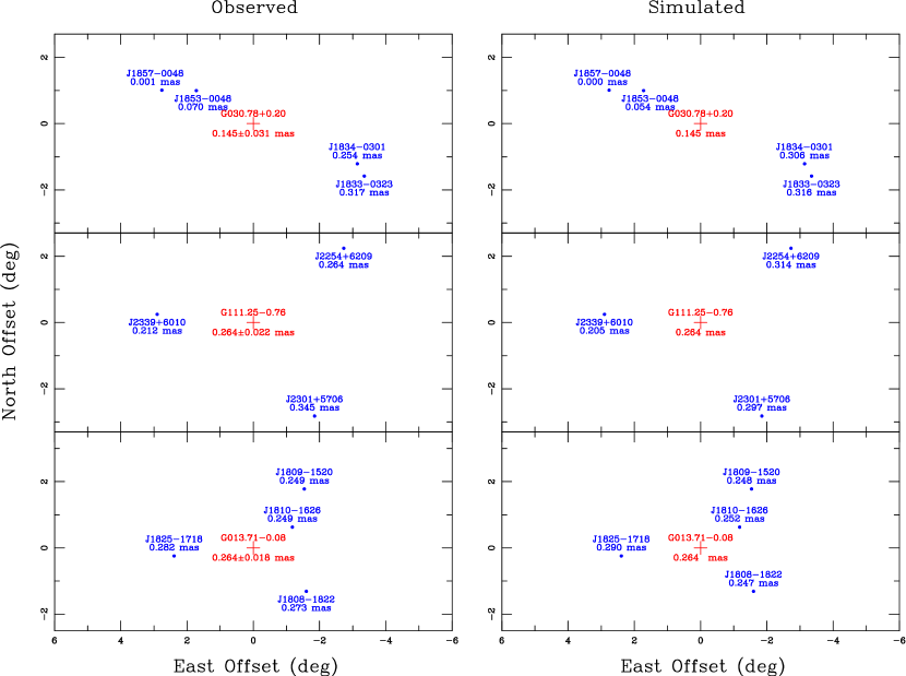
Figure 1: Locations of quasars (filled circles) which served as background reference sources for parallax measurements of three different Galactic 6.7-GHz methanol masers (red plus signs). Left Panels: Individual parallax estimates for the maser relative to each quasar are indicated below the quasar name. The final parallax for the maser using Method-2 to generate an artificial quasar at the position of the maser is given below the maser name. Right Panels: Simulations of parallax measurement for the source groupings, assuming that relative position measurements have been affected by systematic gradients across the sky. The simulations assume relative position measurements are shifted in a planar fashion with a gradient of 0.1 mas per degree of offset on the sky, with randomly different orientations for each of four epochs used to fit parallax. Top Panels: Results for the maser G030.76+0.20. The quasars straddle the maser in a nearly linear arrangement and show a large parallax gradient across their distribution. Middle Panel: Results for the maser G111.25-0.76. There is a moderate gradient in the individual quasar parallax estimates from northeast to southwest. Bottom Panel: Results for the maser G013.71-0.08. This is a case with little or no gradient in parallax.

The left panels of Fig. 1 show a range of examples for parallaxes of 6.7-GHz masers as measured against different quasars as a function of the locations of the quasars relative to the Galactic maser. Of course, being at very great distances, all quasars used as background sources should yield the same parallax for the target maser within measurement uncertainty. However, separate parallax measurements for a maser based on different quasars typically showed a “parallax gradient” on the sky with lower parallaxes for quasars on one side of the maser and larger parallaxes for quasars on the other side. These parallax differences usually significantly exceeded expected parallax uncertainties. Also, parallaxes measured against quasars that projected close together on the sky (e.g., within $\approx 1^{\circ}$) generally yielded similar values. All of these findings argue against quasar structural variability as a significant contributing factor to parallax differences.

We hypothesize that at each epoch uncompensated propagation delays resulted in systematic errors in the measured relative position shifts between maser and quasar, and, even if these errors are uncorrelated at different epochs, they affect the parallax and proper motion estimates, especially when only a small number of observations are used. In order to test this hypothesis, we simulated the effects of a planar relative-position “wedge,” characterized by a position gradient on the sky, ${\partial p}\over{\partial\theta}$, oriented at position angle East of North, $\phi$. This results in a relative (East,North) position shift of $(\delta x,\delta y)=({{\partial p}\over{\partial\theta}}~{}\sin{\phi}~{}\Theta_{x},{{\partial p}\over{\partial\theta}}~{}\cos{\phi}~{}\Theta_{y}),$ where ($\Theta_{x},\Theta_{y}$) is the separation of a background quasar from the target maser source.

We assumed that the position angles of the wedges were uncorrelated among observing epochs and chose different values at each epoch from a uniform random distribution. We then fitted these simulated position shifts for our standard four-epoch observing sequence, which symmetrically sampled the peaks of the Right Ascension parallax signature (see Section 4 for an example). After some experimentation, we found that a characteristic value ${{\partial p}\over{\partial\theta}}=0.1$ mas deg^-1 yielded parallax gradients similar to those we observed. Adopting this value, we changed the random number generator seed used to set the position angles of the wedges and simulated parallax measurements for each of the three configurations of sources. In the right panels of Fig. 1, we show examples that roughly match the real observations. Typically, we needed less than five simulations to find such matches, with each simulation giving two results by reversing the signs of the parallax offsets (i.e., corresponding to a 180^∘ rotation of the position angles of the wedges). We conclude that a position gradient on the sky of $\sim 0.1$ mas deg^-1 with a random orientation at each epoch can explain the variation in our 6.7-GHz parallax results of $\approx 0.01$ to $\approx 0.05$ mas deg^-1 for a maser source relative to background quasars.

As discussed earlier, there is strong circumstantial evidence that uncompensated ionospheric delays are at the root of the relative position wedges. However, the details of how this happens are not clear. The VLBA antennas span about 90^∘ in longitude, or six hours of solar hour-angle, which should result in significant differences in ionospheric conditions above many of the antennas. Thus, one might expect that the effects of ionospheric delays would be only partially correlated among the different sites and would somewhat “average out” in an image made with the entire array over a 6-hour observation. However, it is likely that the total electron content models used to remove most of the ionospheric delays may systematically over or under estimate the electrons, leading to significant correlations in the residual (uncompensated) delays and enhancing relative position shifts. While this should be investigated in the future, it is beyond the scope of this paper, which is primarily concerned with a mitigation strategy to improve parallax accuracy regardless of the cause of the problem.

3 Analysis Methods

In order to deal with the problem of position gradients across our sources, we take advantage of their distribution on the sky. Rioja et al. (2017) recently demonstrated a technique called “MultiView” that uses a two-dimensional interpolation of interferometer phase from a distribution of sources to calibrate phase towards a central target source. They have shown impressive astrometric results at a frequency of 1.6 GHz, where ionospheric effects are more severe than for our observations at 6.7 GHz. Unfortunately, the BeSSeL Survey observations were not conducted in a manner that allows direct use of MultiView calibration. The background quasars were selected to be close to the target, which generally required weak sources that could only be detected in images that combined data from multiple baselines and spanning hours of observation. However, we can use a variant of MultiView with positions measured from images to improve our astrometric accuracy.

Conceptually, one could take the relative position measurements (maser minus quasar) at each epoch and estimate what would be the measurement relative to an “artificial quasar” near or at the position of the maser, and then fit the artificial quasar positional data to estimate parallax and proper motion of the maser. The simplest approach would be to average the positions of all quasars (relative to the maser) to generate the artificial quasar data at each epoch. However, this would not take into account the distribution of the quasars with respect to the maser. Given the quasi-linear behavior on the sky of the parallax results, a better method is to allow for a gradient in relative position as a function of separation from the maser. We investigated two such methods.

Method-1 fits a plane through the 2-dimensional relative-position measurements. Specifically, given the measured position of the $j^{th}$ quasar relative to the maser at epoch $i$, $(x^{j}_{i},y^{j}_{i})$, and the separation on the sky of that quasar relative to the maser, $(\Theta_{x}^{j},\Theta_{y}^{j})$, we fitted the components of the measured positions with the model

$${x^{j}_{i}}=S^{x}_{x}{\Theta_{x}^{j}}+S^{x}_{y}{\Theta_{y}^{j}}+C^{x}~{}~{},$$

and

$${y^{j}_{i}}=S^{y}_{x}{\Theta_{x}^{j}}+S^{y}_{y}{\Theta_{y}^{j}}+C^{y}~{}~{}.$$

In Eqs.  (1) and (2), the $S$ (slope) parameters allow for a tilt of the plane and the $C$ (constant) parameters give the estimated position of the artificial quasar at the maser position. The superscript for the $S$ parameters indicates the component of data being modeled, whereas the subscript indicates the direction of separations for which the slope parameter applies. Fitting this model requires at least three quasars, since for each direction on the sky there are three parameters. A drawback of this method is that the parameters can become degenerate as the quasars approach a linear distribution on the sky.

Table 1: Parallax Results by Method

Source	Standard Parallax	Method-2 Parallax
	(mas)	(mas)
G030.78$+$0.20	$0.161\pm 0.062$	$0.145\pm 0.031$
G111.25$-$0.76	$0.272\pm 0.031$	$0.264\pm 0.022$
G013.71$-$0.08	$0.262\pm 0.015$	$0.264\pm 0.018$

Note. — Comparison of estimated parallaxes for two methods for three representative examples. Column 2 gives standard fitting results, where multiple background quasars are assumed to give the same parallax and effectively averaged together. Column 3 uses “Method-2” (described in the text), where the position of an artifical quasar at the target maser position is generated at each epoch and used for fitting parallax; these uncertaintes have been inflated by 10% as discussed in Section 4 .

Method-2 assumes that the $x$-components of the measured position differences depend only on the $x$-separations of the quasars from the maser on the sky (and the same for the $y$-components):

$${x^{j}_{i}}=S^{x}_{x}{\Theta_{x}^{j}}+C^{x}~{}~{},$$

and

$${y^{j}_{i}}=S^{y}_{y}{\Theta_{y}^{j}}+C^{y}~{}~{}.$$

This method has only two parameters per coordinate and hence only requires two quasars at a minimum to work, and if more quasars are available one will get a more robust artificial quasar data. This method also allows for linear distributions of quasar on the sky, which in principle could yield excellent artificial quasar data. Using this method, we generated artificial quasar data at each epoch and used these to fit for parallax and proper motion of the masers. The parallax values generated in this fashion are indicated in the left panels of Fig. 1. Based on a visual inspection of the three cases presented, these give reasonable values.

Table 1 lists the parallax results for the three examples shown in Fig. 1 both for a standard fitting approach, where all background quasars are assumed to yield the same parallax for the target maser, and for the fitting approach of Method-2 described above. In both cases, the parallax uncertainties are estimated from the magnitude of the post-fit residuals. For these three examples, Method-1 and Method-2 returned parallax values within a few micro-arcseconds of each other and nearly identical formal uncertainties. However, in some other cases, Method-1 gave larger formal uncertainties. Because of this, and because Method-1 requires solving for more parameters, we adopted the simpler Method-2 over Method-1 for our application.

As is evident in Fig. 1, G030.78$+$0.20 displays an unusually large parallax gradient on the sky, and the parallax uncertainty from Method-2 artificial quasar data is 50% that of the standard method. The source G111.25$-$0.76 displays a moderate parallax gradient on the sky, and the artifical quasar uncertainty is 70% that of the standard estimate. In the final example, G013.71$-$0.08, little or no parallax gradient is detected and the standard and artificial quasar methods produce similar results. Since, in the presence of significant parallax gradients, the artifical quasar (Method-2) almost always gave smaller post-fit residuals than from a simple combined fit using all quasars, which does not take into account possible position gradients on the sky, we adopted it as the method of choice for the BeSSeL Survey 6.7-GHz data.

4 Other Considerations

When we planned BeSSeL Survey observations for VLBA programs BR149 and BR198, we scheduled the minimum number of epochs for parallax and proper motion observations, which would yield uncorrelated parameter estimates and the lowest parallax uncertainty. This could be accomplished with four epochs scheduled to sample the peaks of the parallax signature in Right Ascension, for example, for sources at low Galactic longitude we would schedule one observation in March, two in September, and one in the following March. We optimized based on the Right Ascension component of the parallax signature, since 1) that component has a larger amplitude than the Declination component for most Galactic sources, and 2) VLBA measurements are generally more accurate for that component than for the Declination component (Reid et al., 2009).

By observing three or four quasars for each maser target, we planned to have sufficient degrees of freedom to estimate true astrometric accuracy from the magnitudes of the residuals to the parallax fits. For example, with four background quasars for a maser target and four epochs of observations, there are 16 relative position measurements in the critical Right Ascension direction. Since all background quasars should yield the same parallax and motion for the maser, each additional quasar only adds one extra parameter, a correction to its position offset, while adding four extra data points. Thus, for this example, there would be 16 data points and 6 parameters to solve for, yielding 10 degrees of freedom.

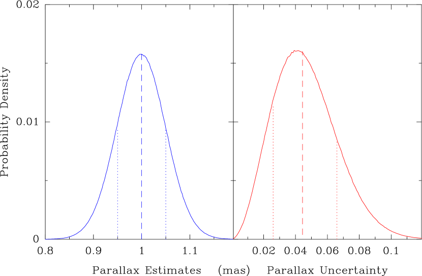
Figure 2: Results of $10^{7}$ simulations of parallax estimates which used four optimally sampled measurements of the Right Ascension difference between a maser and a background quasar. Data were simulated for a parallax of 1.00 mas and single-epoch position measurement uncertainty of 0.10 mas, which should yield a fitted parallax uncertainty of 0.05 mas. Binned histograms tracing probability density functions (PDF) are shown with solid lines; median values are indicated with dashed lines and the 68% confidence ranges are indicated with dotted lines. Left Panel: PDF for the parallax trials, which return the expected estimates of parallax. Right Panel: PDF for the formal parallax uncertainties, scaled by the post-fit residuals to give unity reduced chi-squared values. This PDF is asymmetric with mean and median values for the uncertainty $\approx 10$% below the correct value of 0.05 mas and a tail toward larger values. The symmetric 68% confidence range is 0.026 to 0.066 mas (uncorrected for bias).

However, in order to mitigate the effects of position gradients across our source groupings, we used up most of our degrees of freedom to generate the artificial quasar data. Fits to this data for four epochs have only one degree of freedom when the Right Ascension data dominates. This in no way biases the parallax estimates, but it leads to uncertain estimates for the uncertainty in the parallax. Fig. 2 shows the results of $10^{7}$ simulated parallax fits with only one degree of freedom (i.e., using 4 optimally sampled data points and 3 parameters). The true parallax value was set at 1.00 mas and the Right Ascension ($1\sigma$) position uncertainty was set to 0.10 mas. These values should lead to a true parallax uncertainty of 0.05 mas, since we actually measure twice the parallax amplitude. The left panel of the figure shows that we retrieve the correct values and there is no bias in the parallax estimate. The right panel shows the distribution of formal parallax uncertainties, estimated from the scatter in the post-fit residuals. The probability density is asymmetric with mean and median values of $\approx 0.0444$ mas (about 10% below the correct value of 0.05) and a tail to larger values. Being conservative, we have inflated our parallax uncertainties accordingly to remove this slight bias. Following this correction, the symmetric 68% confidence range for the parallax uncertainties for this example spans from 0.029 to 0.073 mas about the correct value of 0.05 mas. Thus, the uncertainty in the uncertainty can be expected to be significant ($\pm 44$%). In conclusion, even though the parallax estimate is unbiased, one should exercise caution when using the estimate of its uncertainty from our 6.7-GHz parallax measurements.

Facilities: VLBA

References

- Honma, Tamura & Reid (2008) Honma, M., Tamura, Y. & Reid, M. J. 2008, PASJ, 60,, 951
- Reid et al. (2009) Reid, M. J., Menten, K. M., Brunthaler, A. et al. 2009, ApJ, 693, 397
- Reid et al. (2014) Reid, M. J., Menten, K. M., Brunthaler, A. et al. 2014, ApJ, 783, 130
- Reid & Honma (2014) Reid, M. J. & Honma, M. 2014, ARA&A, 52, 339
-
Walker & Chatterjee (1999)
Walker & Chatterjee 1999, VLBA Scientific Memo 23,
https://library.nrao.edu/vlbas.shtml - Rioja et al. (2017) Rioja, M. J., Dodson, R., Orosz, G., Imai, H. & Frey, S. 2017, AJ, 153, 105