Unphysical poles and dispersion relations for Möbius domain-wall fermions in free field theory at finite $L_{s}$

Abstract

We find that the quark propagator constructed from the domain-wall fermion operator has $L_{s}-1$ extra poles as well as the pole that realizes the physical quark in the continuum limit. We show the energy-momentum dispersion relation for the physical and unphysical poles of Möbius domain-wall fermions in free field theory at finite $L_{s}$. The dependence of extra pole energies on the Möbius parameter $b-c$ and on the domain-wall height $M_{5}$ is investigated. Our result suggests that small values of $b-c$ set a large lower bound on the unphysical pole masses and the contribution of these poles could be suppressed well by calculating with small $b-c$.

I Introduction

Introducing the charm quark into lattice simulation is desired to provide accurate Standard Model predictions for flavor physics, which enable us to probe for new physics beyond the Standard Model. Especially, the non-perturbative calculation of quantities associated with the Glashow-Iliopoulos-Maiani (GIM) mechanism Glashow:1970gm such as the $K_{L}$–$K_{S}$ mass difference ($\Delta M_{K}$) essentially needs the charm quark to cancel the divergent contributions of up-quark loop diagrams. Because of the large charm-quark mass $m_{c}$ compared to the typical scale of QCD, a lattice calculation including a charm quark encounters a scale problem. Namely, the lattice cutoff $a^{-1}$ needs to be sufficiently larger than $m_{c}$ to safely control the discretization error arising from $am_{c}$, while the box size $L$ is usually required to obey $m_{\pi}L\gtrsim 4$, with the pion mass $m_{\pi}$, to avoid uncontrollable finite volume effects. Thus, lattice calculation at the physical pion and charm quark masses is a challenging task for the currently available computational resources.

This work is devoted to investigating properties of the discretization effects appearing in Möbius domain-wall fermions Brower:2004xi ; Brower:2012vk , an extension of Shamir domain-wall fermions Kaplan:1992bt ; Shamir:1993zy , at heavy quark masses. Although the charm quark completely violates chiral symmetry due to its heavy mass, introducing the charm quark as a domain-wall fermion is still necessary to achieve an accurate GIM cancellation if the light quarks are implemented with a domain-wall fermion formulation, which appropriately preserves the chiral symmetry of the light quarks. There have been several works on $D$ meson decay constants using domain-wall fermions Chen:2014hva ; Boyle:2017jwu and overlap fermions for valence quarks and domain-wall fermions for sea quarks Yang:2014sea . A lattice simulation including $2+1+1$ optimal domain-wall fermions Chiu:2002ir was implemented Chen:2017kxr and was the first study with a dynamical domain-wall charm quark. In addition, the RBC and UKQCD collaborations are pursuing the calculation of the $\Delta M_{K}$ Bai:2014cva ; Christ:2014qwa , $\varepsilon_{K}$ Christ:2014qwa ; Bai:2016gzv , rare kaon decays $K\rightarrow\pi l^{+}l^{-}$ Christ:2015aha ; Christ:2016mmq and $K\rightarrow\pi\nu\bar{\nu}$ Christ:2016eae ; Bai:2017fkh , which are all associated with the GIM mechanism and quite sensitive to the discretization effects due to the charm-quark mass.

The charm quark treated in the domain-wall fermion formulation is supposed to have some special difficulties in addition to the naïve $O(a^{2}m^{2}_{c})$ discretization errors and beyond. The seminal work on domain-wall fermions at large quark masses Liu:2003kp ; Christ:2004gc investigated the hermitian version of the domain-wall operator, the five-dimensional Dirac operator multiplied by the chirality operator $\gamma_{5}$ and the five-dimensional reflection operator. It found that the hermitian operator contains unphysical modes whose eigenvalues are largely independent of the input quark mass. This fact indicates that as the input quark mass approaches the cutoff the contribution of physical modes will be contaminated by unphysical modes.

This unphysical contribution may be related to the oscillatory behavior of domain-wall fermions Dudek:2006ej , which is a particular issue of domain-wall fermions and is observed in correlation functions when a simulation is carried out at large domain-wall heights such as $M_{5}\simeq 1.7$. This unphysical oscillation was understood as the result of negative eigenvalues of the transfer matrix Syritsyn:2007mp , which were shown to exist in the region of $M_{5}>1$ in the free field case.

Recently, another description of the origin of the unphysical oscillation was proposed Liang:2013eoa ; Sufian:2016cft . They argued that the four-dimensional quark propagator constructed from the domain-wall fermion operator has an extra pole, whose energy has a non-zero imaginary part ${\rm{i}}\pi$ in lattice units for $M_{5}>1$ in free field theory, leading to an oscillatory behavior of the quark propagator. Their numerical result Sufian:2016cft indicates that the impact of the unphysical oscillation could be reduced by choosing $M_{5}$ and the Möbius parameters $b$ and $c$ to satisfy $M_{5}(b-c)<1$ and that the Boriçi domain-wall fermion Borici:1999zw ($b=c$) is optimal to suppress the unphysical oscillation. Although this viewpoint of an unphysical pole is quite impressive and provides a clear interpretation of the unphysical effects of domain-wall fermions, we find that when examined in detail their description Liang:2013eoa ; Sufian:2016cft is not correct. Especially, we find there are $L_{s}-1$ unphysical poles, while they found only one.

To motivate the presence of this collection of unphysical poles, it may be helpful to consider the case of overlap fermions, which has the same quark propagator as domain-wall fermions in the limit of infinite $L_{s}$ up to a contact term and a normalization factor. The overlap Dirac operator is given by

$$D_{\rm ov}=\frac{1}{2}+\frac{1}{2}\gamma_{5}\frac{H}{\sqrt{H^{2}}},$$ (1)

with a hermitian kernel $H$. The corresponding propagator contains $\sqrt{H^{2}}$ and becomes ambiguous in the region where $H^{2}$ is not positive definite, resulting in the presence of an unphysical brunch cut for an imaginary value of Euclidean momentum variable $p_{4}$. In this paper, we demonstrate the presence of $L_{s}-1$ unphysical poles for finite $L_{s}$ as the counterpart of this brunch cut.

We also examine the fundamental properties of the unphysical poles of domain-wall fermions by showing the dispersion relation for the physical and unphysical poles in free field theory at finite $L_{s}$. We find that the range of unphysical pole energies significantly depends on $M_{5}$ and $b-c$ as well as on the spatial momentum and that small values of $b-c$ set a large lower bound on the unphysical pole energies, possibly suppressing the contribution of the unphysical poles. Since this range of unphysical pole energies is found to be independent of the physical quark mass, numerical calculation with heavy quarks would be contaminated by unphysical poles as the physical quark mass approaches the lower bound of the unphysical pole region.

The paper is organized as follows. In Section II, we give definitions and some comments on the parameters of Möbius domain-wall fermions. In Section III, we give the five- and four-dimensional propagators of Möbius domain-wall fermions. In Section IV, we show the presence of unphysical poles of domain-wall fermions as well as the physical pole. In Section V, we show the dispersion relation for the physical and unphysical poles and discuss the dependence of unphysical pole energies on the parameters of Möbius domain-wall fermions. In Section VI, we conclude this paper and give some discussion. In Appendix A, we discuss a connection with overlap fermions and demonstrate that domain-wall fermions in the limit of infinite $L_{s}$ and overlap fermions have an unphysical branch cut instead of unphysical poles. In Appendix B, we give the five- and four-dimensional propagators in some special cases, in which the usual form of these propagators is irrelevant.

II Möbius domain-wall fermions

In this study, we work in the momentum space, where the lattice action of a Möbius domain-wall fermion is given by

$$S=\sum_{s,t=0}^{L_{s}-1}\sum_{p}\overline{\psi}_{s}(-p)(D_{\rm MDW})_{s,t}\psi_{t}(p).$$ (2)

Here, $\overline{\psi}_{s}(-p)$ and $\psi_{t}(p)$ are the five-dimensional Möbius domain-wall fermion fields labeled by the four-dimensional momentum variables, $-p$ and $p$, and the indices for the fifth direction, $s,t=0,1,\ldots,L_{s}-1$. We employ the convention used by the RBC and UKQCD collaborations Blum:2014tka , in which the corresponding Dirac operator is defined by

$$D_{\rm MDW} =\left(\begin{array}[]{cccccc}\tilde{D}&-P_{-}&0&\ldots&0&mP_{+}\\ -P_{+}&\tilde{D}&-P_{-}&\ddots&0&0\\ 0&-P_{+}&\tilde{D}&\ddots&\ddots&\vdots\\ \vdots&\ddots&\ddots&\ddots&-P_{-}&0\\ 0&0&\ddots&-P_{+}&\tilde{D}&-P_{-}\\ mP_{-}&0&\ldots&0&-P_{+}&\tilde{D}\end{array}\right).$$ (9)

Here, we define the chiral projection operators $P_{\pm}=\frac{1}{2}(1\pm\gamma_{5})$ and

$$\tilde{D}=D_{-}^{-1}D_{+},\ \ D_{+}=1+bD_{W},\ \ D_{-}=1-cD_{W},$$ (10)

with the Wilson Dirac operator $D_{W}$ in the momentum space at a negative mass parameter $-M_{5}$,

$$D_{W}={\rm{i}}\hbox to0.0pt{\hbox to5.55557pt{\hfil/\hfil}\hss}\tilde{p}+\sum_{\mu}(1-\cos p_{\mu})-M_{5},$$ (11)

where $\hbox to0.0pt{\hbox to5.55557pt{\hfil/\hfil}\hss}\tilde{p}=\sum_{\mu}\gamma_{\mu}\sin p_{\mu}$. For simplicity, we omit the lattice spacing $a$ and everything is expressed in lattice units throughout this paper.

We define the corresponding four-dimensional quark fields by

$$q=P_{-}\psi_{0}+P_{+}\psi_{L_{s}-1},\ \ \overline{q}=\overline{\psi}_{0}P_{+}+\overline{\psi}_{L_{s}-1}P_{-}.$$ (12)

As shown in Brower:2012vk ; Blum:2014tka , the four-dimensional quark propagator constructed from these fields $S_{F}^{4d}(p)=\langle q(-p)\overline{q}(p)\rangle$ in the limit $L_{s}\rightarrow\infty$ is the same as that in the corresponding overlap action up to a contact term and a normalization factor.

The action has five input parameters in total: the mass parameter $m$, the extent of the fifth dimension $L_{s}$, the domain-wall height $M_{5}$, the Möbius parameters $b$ and $c$. Except for the mass parameter $m$, these are parameters of the regularization and do not affect any observables in the continuum limit. Therefore we can tune them to minimize unwanted discretization effects. As is well known, the fifth-dimensional extent $L_{s}$ determines the amount of violation of chiral symmetry on the lattice, which is usually quantified by the residual mass $m_{\rm res}$ and vanishes in the limit $L_{s}\rightarrow\infty$. The domain-wall height $M_{5}$ determines the scale for the exponential locality of the four-dimensional effective fermion field Hernandez:1998et ; Kikukawa:2000kd and is also related to $m_{\rm res}$ Aoki:2002vt . The optimal choice of $M_{5}$ is 1 for the case of the free field, while that in the non-perturbative case has been studied by analyzing the spectral flow on some representative configurations to minimize $m_{\rm res}$ Aoki:2002vt ; Antonio:2008zz ; Hagler:2007xi ; WalkerLoud:2008bp . The obtained best choice was $M_{5}=1.7$–$1.8$ depending on the detail of the lattice setup. By applying link smearing, the residual mass may be better controlled and the optimal choice of $M_{5}$ could be moved to 1 Cho:2015ffa . In addition, the $M_{5}$-dependence of the amount of discretization error for the heavy-heavy decay constant was investigated, resulting in a slightly smaller tuned value $M_{5}=1.6$ Boyle:2016imm . The Möbius scale $b+c$, which is proportional to the Möbius kernel, has also been tuned to minimize $m_{\rm res}$, while the dependence on $b-c$ has not been studied a lot. In this work, we investigate how the significance of the unphysical modes depends on these parameters including $b-c$.

III Quark propagator at finite $L_{s}$

The five-dimensional Dirac operator $D_{\rm MDW}$ can be rewritten as

$$D_{\rm MDW}={b+c\over D_{-}^{\dagger}D_{-}}{\rm{i}}\hbox to0.0pt{\hbox to5.55557pt{\hfil/\hfil}\hss}\tilde{p}+W^{+}P_{-}+W^{-}P_{+},$$ (13)

where

$$W^{\pm}_{s,t} =W\delta_{s,t}-\delta_{s\pm 1,t}+m\delta_{s/t,L_{s}-1}\delta_{t/s,0},$$ (14)

$$W ={-bc(\tilde{p}^{2}+{\cal M}^{2})+(b-c){\cal M}+1\over D_{-}^{\dagger}D_{-}},$$ (15)

$${\cal M} =\sum_{\mu}(1-\cos p_{\mu})-M_{5},$$ (16)

$$D_{-}^{\dagger}D_{-} =c^{2}(\tilde{p}^{2}+{\cal M}^{2})-2c{\cal M}+1,$$ (17)

with $\tilde{p}^{2}=\sum_{\mu}\sin^{2}p_{\mu}$. Thus, we can calculate the five-dimensional propagator of Möbius domain-wall fermions in the same way Shamir:1993zy as for Shamir domain-wall fermions. We obtain

$$D^{-1}_{\rm MDW} =\left[-{b+c\over D_{-}^{\dagger}D_{-}}{\rm{i}}\hbox to0.0pt{\hbox to5.55557pt{\hfil/\hfil}\hss}\tilde{p}+W^{-}\right]G^{-}P_{-}+\left[-{b+c\over D_{-}^{\dagger}D_{-}}{\rm{i}}\hbox to0.0pt{\hbox to5.55557pt{\hfil/\hfil}\hss}\tilde{p}+W^{+}\right]G^{+}P_{+},$$ (18)

$$G^{\pm} =\left[\bigg{(}{b+c\over D_{-}^{\dagger}D_{-}}\bigg{)}^{2}\tilde{p}^{2}+W^{\mp}W^{\pm}\right]^{-1}\equiv(Q^{\pm})^{-1},$$

$$G^{\pm}_{s,t} =A_{0}{\rm{e}}^{-\alpha|s-t|}+A_{\pm}{\rm{e}}^{\alpha(s+t-L_{s}+1)}+A_{\mp}{\rm{e}}^{-\alpha(s+t-L_{s}+1)}+A_{m}\cosh[\alpha(s-t)],$$ (19)

$$\cosh\alpha =\frac{\big{(}{b+c\over D_{-}^{\dagger}D_{-}}\big{)}^{2}\tilde{p}^{2}+W^{2}+1}{2W},$$ (20)

$$A_{0} =\frac{1}{2W\sinh\alpha},$$ (21)

$$A_{\pm} =\frac{A_{0}}{F_{L_{s}}}(1-m^{2})(W-{\rm{e}}^{\mp\alpha}),$$ (22)

$$A_{m} =\frac{A_{0}}{F_{L_{s}}}\left[4mW\sinh\alpha-2(W{\rm{e}}^{-\alpha}-1+m^{2}(1-W{\rm{e}}^{\alpha})){\rm{e}}^{-\alpha L_{s}}\right],$$ (23)

$$F_{L_{s}} ={\rm{e}}^{\alpha L_{s}}(1-W{\rm{e}}^{\alpha}+m^{2}(W{\rm{e}}^{-\alpha}-1))-4mW\sinh\alpha$$

$$\hskip 11.38109pt+{\rm{e}}^{-\alpha L_{s}}(W{\rm{e}}^{-\alpha}-1+m^{2}(1-W{\rm{e}}^{\alpha})).$$ (24)

Since the four-dimensional effective fields $q$ and $\overline{q}$ are given by (12), the four-dimensional quark propagator $S_{F}^{4d}(p)=\langle q(-p)\overline{q}(p)\rangle$ constructed from the Möbius domain-wall fermions is written as

$$S_{F}^{4d}(p) =P_{-}(D_{\rm MDW}^{-1})_{0,0}P_{+}+P_{+}(D_{\rm MDW}^{-1})_{L_{s}-1,L_{s}-1}P_{-}$$

$$\hskip 11.38109pt+P_{-}(D_{\rm MDW}^{-1})_{0,L_{s}-1}P_{-}+P_{+}(D_{\rm MDW}^{-1})_{L_{s}-1,0}P_{+}$$

$$={2\sinh(\alpha L_{s})\over F_{L_{s}}}{b+c\over D_{-}^{\dagger}D_{-}}{\rm{i}}\hbox to0.0pt{\hbox to5.55557pt{\hfil/\hfil}\hss}\tilde{p}$$

$$\hskip 11.38109pt+{2\over F_{L_{s}}}\left\{m[W\sinh(\alpha(L_{s}-1))-\sinh(\alpha L_{s})]-W\sinh\alpha\right\}.$$ (25)

In the limit of infinite $L_{s}$, this four-dimensional propagator becomes

$$S_{F}^{4d}(p)\xrightarrow{\ L_{s}\rightarrow\infty\ }\frac{{b+c\over D_{-}^{\dagger}D_{-}}{\rm{i}}\hbox to0.0pt{\hbox to5.55557pt{\hfil/\hfil}\hss}\tilde{p}+m(W{\rm{e}}^{-\alpha}-1)}{1-W{\rm{e}}^{\alpha}+m^{2}(W{\rm{e}}^{-\alpha}-1)}.$$ (26)

Since the Möbius scale $b+c$ is associated only with $L_{s}$-dependence, the propagator in the limit of infinite $L_{s}$ (26) must be independent of $b+c$, despite its apparent dependence on that combination. The $b+c$-independent form is given in (34).

The four-dimensional quark propagator (25) at finite $L_{s}$ is quite different from that given in Sufian:2016cft . This may originate from the slight difference in $F_{L_{s}}$. Since the coefficients (22) and (23) are determined through the boundary conditions (45)–(48) for the fifth direction, the validity of these coefficients and $F_{L_{s}}$ given in this section can be checked by inserting $G^{\pm}_{s,t}$ into the boundary conditions.

IV Physical and unphysical poles at finite $L_{s}$

It is well known that the quark propagator $S_{F}^{4d}$ has a physical pole that reproduces an appropriate Dirac fermion in the continuum limit. This can be verified by expanding the denominator of the quark propagator with respect to the momentum variable. In the case of infinite $L_{s}$, the denominator of $S_{F}^{4d}$ in (26) is expanded as

$$1-W{\rm{e}}^{\alpha}+m^{2}(W{\rm{e}}^{-\alpha}-1)=-\frac{(b+c)\big{[}M_{5}^{2}(2-(b-c)M_{5})^{2}m^{2}+p^{2}\big{]}}{M_{5}(2-(b-c)M_{5})(1+cM_{5})^{2}}+O(p^{4},m^{2}p^{2}).$$ (27)

Thus, the mass $m_{f}^{\rm pole}$ of the physical pole is approximated at $M_{5}(2-(b-c)M_{5})m$ for a light quark and is generally different from the input mass $m$ even in the case of infinite $L_{s}$. In this work, we input $m_{f}^{\rm pole}$ and tune the parameter $m$ to realize the pole mass $m_{f}^{\rm pole}$.

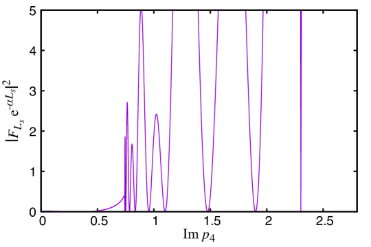
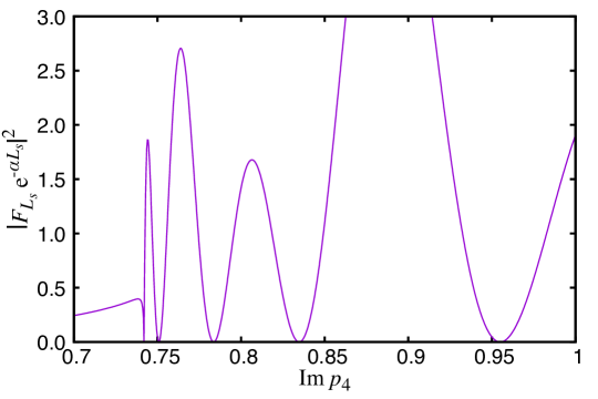
Figure 1: $|F_{L_{s}}{\rm{e}}^{-\alpha L_{s}}|^{2}$ calculated at $L_{s}=8$, $M_{5}=0.9$, $m_{f}^{\rm pole}=0.35$, $b-c=1$, $b+c=1$, $\vec{p}=0$ and ${\rm Re}~{}p_{4}=0$ plotted as a function of ${\rm Im}~{}p_{4}$. The lower two panels are magnifications of complicated parts in the top panel, which accommodates all the zero points of $F_{L_{s}}$.

Besides this physical pole, we find that $F_{L_{s}}$ has other zero points, which could give an unphysical contribution to four-dimensional physics. Figure 1 shows $|F_{L_{s}}{\rm{e}}^{-\alpha L_{s}}|^{2}$ calculated with Shamir domain-wall fermions at $L_{s}=8$, $M_{5}=0.9$, $m_{f}^{\rm pole}=0.35$, $\vec{p}=0$ and ${\rm Re}~{}p_{4}=0$. While the physical pole is seen at ${\rm Im}~{}p_{4}=m_{f}^{\rm pole}=0.35$, there are nine other zero points of $F_{L_{s}}$. Two of them are trivially identified as the points satisfying $\cosh\alpha=1$ or $\cosh\alpha=-1$, which correspond to ${\rm Im}~{}p_{4}\simeq 2.30$ and 0.74 in the plot, respectively. Between these two zero points, the seven other zero points are found. All of the zero points in this parameter choice are located on the imaginary axis of $p_{4}$.

In Liang:2013eoa ; Sufian:2016cft , one of the trivial zero points satisfying $\cosh\alpha=1$ was regarded as the unphysical pole of domain-wall fermions. However, the vanishing of $F_{L_{s}}$ at $\cosh\alpha=\pm 1$ does not mean the presence of unphysical poles at these points because the numerator of the quark propagator (25) also vanishes at these points and one can verify the limit $\lim_{\alpha\rightarrow 0,{\rm{i}}\pi}S_{F}^{4d}(p)$ is still finite. In fact, the original $L_{s}\times L_{s}$ matrix $Q^{\pm}=(G^{\pm})^{-1}$ is still regular, ${\rm det}~{}Q^{\pm}\neq 0$, even at these points. This confusion may originate from the fact that the functional form of the inverse matrix (19) is invalid for some special cases, $\cosh\alpha=\pm 1$ or $W=0$, and the inverse matrix $G_{s,t}^{\pm}$ in these special cases has another functional form as given in Appendix B.

The quark propagator at each of the remaining seven zero points between these special zero points has a real singularity. These zero points may give a significant lattice artifact when the calculation is done at a large value of $m_{f}^{\rm pole}$. We regard these zero points as the unphysical poles. Note that these unphysical poles are located in the region $-1<\cosh\alpha<1$, in which $\alpha$ is pure imaginary and any terms in (24) are not suppressed at large $L_{s}$, showing some oscillatory behavior with varying ${\rm Im}~{}p_{4}$. As the extent of the fifth direction $L_{s}$ increases, the number of these oscillations also increases, leading to the presence of more unphysical poles. In our analysis, there are always $L_{s}-1$ unphysical poles. In the limit of infinite $L_{s}$, an unphysical branch cut appears instead of a series of unphysical poles as shown in Appendix A.

In the following section, we discuss the fundamental properties of these unphysical poles by showing the energy-momentum dispersion relation at various input parameters.

V Dispersion relations

As mentioned in the previous section, the quark propagator (25) at finite $L_{s}$ has $L_{s}-1$ unphysical poles as well as the physical pole. In this section, we discuss the properties of the unphysical poles and the best choice of the Möbius parameters to suppress them, by analyzing the dispersion relation for these poles in free field theory. While it is likely familiar to the reader, for completeness we point out that although lattice calculations are performed in Euclidean space with $\tilde{p}^{2}=\sum_{\mu}\sin^{2}p_{\mu}>0$ it is the location of poles at negative values of $p^{2}_{4}$ that determines the physical energies $E(\vec{p}\,)=$ Im $p_{4}(\vec{p}\,)$ of the quark states in free field theory. These poles and corresponding energies determine the exponential fall-off of the quark propagators at large Euclidean time separations. The dispersion relation for fermions on the lattice deviate from those for continuum fermions with $O(a^{2})$ error. While dispersion relations for improved overlap fermions using the Brillouin kernel were investigated Cho:2015ffa ; Durr:2017wfi, we concentrate on the dispersion relations for unimproved Möbius domain-wall fermions to investigate another source of cutoff effects due to unphysical poles.

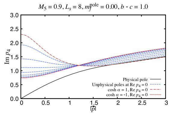
Figure 2: Dispersion relation for the domain-wall fermion at $M_{5}=0.9,L_{s}=8,m_{f}^{\rm pole}=0,b+c=1,b-c=1$ and spatial momentum $\vec{p}=({|\vec{p}\,|\over\sqrt{3}},{|\vec{p}\,|\over\sqrt{3}},{|\vec{p}\,|\over\sqrt{3}})$.

Figure 2 shows the dispersion relation for the domain-wall fermion at $M_{5}=0.9$, $L_{s}=8$, $m_{f}^{\rm pole}=0$, $b=1$ and $c=0$. The spatial momentum is chosen in the diagonal direction, $\vec{p}=({|\vec{p}\,|\over\sqrt{3}},{|\vec{p}\,|\over\sqrt{3}},{|\vec{p}\,|\over\sqrt{3}})$. In the figure, one physical (solid curve) and seven unphysical poles (dashed curves) are seen on the imaginary axis of $p_{4}$ at any spatial momentum.

As discussed in the previous section, these unphysical poles are confined to the region between two curves, $\cosh\alpha=1$ (dashed-dotted curve) and $\cosh\alpha=-1$ (dotted curve). The boundaries $\cosh\alpha=\pm 1$ are analytically given by

$$\cos p_{4}|_{\cosh\alpha=1} =\frac{\sum_{i=1}^{3}\sin^{2}p_{i}+B^{2}+1}{2B},$$ (28)

$$\cos p_{4}|_{\cosh\alpha=-1} =\frac{4+4(b-c)B+(b-c)^{2}(\sum_{i=1}^{3}\sin^{2}p_{i}+B^{2}+1)}{4(b-c)+2(b-c)^{2}B},$$ (29)

$$B =4-M_{5}-\sum_{i=1}^{3}\cos p_{i}.$$ (30)

The solution of $\cosh\alpha=1$ depends only on $M_{5}$ and $p_{i}$, implying that either of the corresponding lower or upper bounds on the unphysical pole locations depends only on $M_{5}$. On the other hand, the solution of $\cosh\alpha=-1$ depends also on $b-c$ and therefore the other bound on the unphysical pole masses could be controlled by varying $b-c$. Since $b+c$ is not related to the region of unphysical pole energies and is usually tuned to minimize the residual mass, we fix $b+c=1$ and do not vary it in this work.

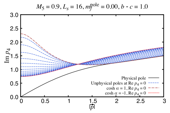
Figure 3: Same as Figure 2 but at $m_{f}^{\rm pole}=0.35$.

Figure 4: Same as Figure 2 but at $L_{s}=16$.

Before varying $M_{5}$ and $b-c$, which play a key role to change the region of unphysical pole energies, we briefly present the results of varying the other parameters $m_{f}^{\rm pole}$ and $L_{s}$. In Figure 4, we show the dispersion relation in a massive case at $m_{f}^{\rm pole}=0.35$. While the physical pole mass has certainly moved to 0.35, the unphysical poles remain at close to their earlier locations when $m_{f}^{\rm pole}=0$. In fact, the boundaries (28) (29) of the unphysical poles are independent of $m_{f}^{\rm pole}$. Therefore, as the physical pole mass $m_{f}^{\rm pole}$ increases and approaches the unphysical pole masses, the dominance of the physical pole would be lost. A similar observation was shown in Liu:2003kp ; Christ:2004gc , which investigated the physical and unphysical modes of the hermitian version of the five-dimensional operator, the Dirac operator multiplied by $\gamma_{5}$ and the reflection operator.

Figure 4 shows the dispersion relation at $L_{s}=16$ and with the same values of the other parameters as those in Figure 2. As described in the previous section, $F_{L_{s}}$ oscillates in the region $-1<\cosh\alpha<1$ with varying the momentum variable and its frequency is proportional to $L_{s}$. Thus, the number of unphysical poles has been increased to 15.

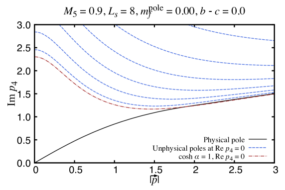
Figure 5: Same as Figure 2 but at $b-c=0.5$.

Figure 6: Same as Figure 2 but at $b-c=0$.

Now we show the results at smaller values of $b-c$. Figure 6 shows the result at $b-c=0.5$. The values of ${\rm Im}~{}p_{4}$ on the curve $\cosh\alpha=-1$ are larger than those for the Shamir type $b-c=1$ and the lower bound on the unphysical pole masses has been increased to $\sim 1.41$. This fact implies that the contribution of unphysical poles at long distances would be suppressed more rapidly. Figure 6 shows the result at $b-c=0$, where ${\rm Im}~{}p_{4}$ with $\cosh\alpha=-1$ is infinitely large as (29) indicates. Thus, small values of $b-c$ make the unphysical modes heavy and realize a small coupling between unphysical poles and the four-dimensional physics.

So far, we have discussed in the case of $M_{5}=0.9<1$, which has the most simple structure of unphysical poles. The case $M_{5}=1$ gives a similar dispersion relation with a slight modification that ${\rm Im}~{}p_{4}$ with $\cosh\alpha=1$ diverges at $\vec{p}=0$ as described by (28).

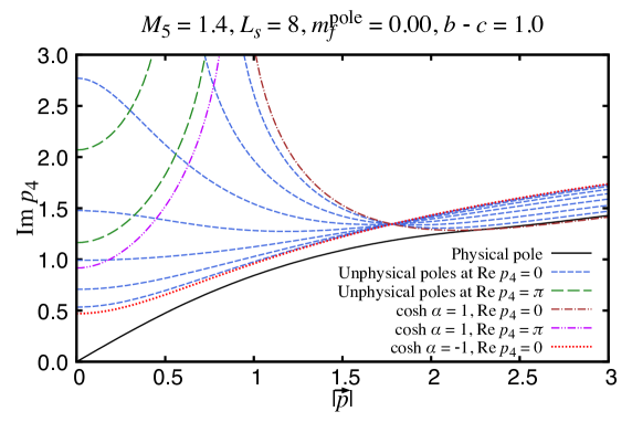
Figure 7: Same as Figure 2 but at $M_{5}=1.4$.

In the case of $M_{5}>1$, $\alpha$ could be pure imaginary at ${\rm Re}~{}p_{4}=\pi$ as well as at ${\rm Re}~{}p_{4}=0$ and therefore some of the unphysical poles are located at ${\rm Re}~{}p_{4}=\pi$. Figure 7 shows the result at $M_{5}=1.4$. The curve of $\cosh\alpha=1$ (dashed-dotted curve) on the imaginary axis blows up at $|\vec{p}|\simeq 0.90$, below which the solution of $\cosh\alpha=1$ (dashed double-dotted curve) is located at ${\rm Re}~{}p_{4}=\pi$. Thus, there are some unphysical poles at ${\rm Re}~{}p_{4}=\pi$ (coarse-dashed curves) at small spatial momenta. As suggested in Liang:2013eoa ; Sufian:2016cft , this kind of unphysical pole may cause unphysical oscillation because the contribution of an unphysical pole at $p_{4}=p_{4}^{\rm pole}$ to the quark propagator for the time direction has a term $\sim{\rm{e}}^{{\rm{i}}p_{4}^{\rm pole}x_{4}}$, which is oscillatory unless ${\rm Re}~{}p_{4}^{\rm pole}=0$.

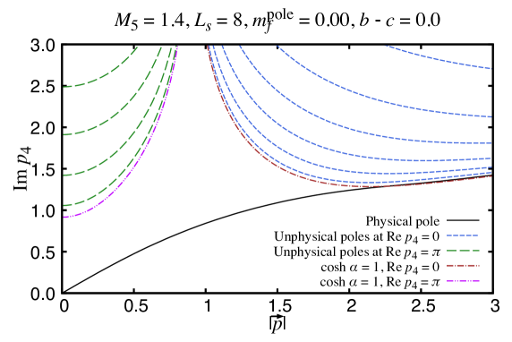
Figure 8: Same as Figure 7 but at $b-c=0$.

In Figure 7, the lower bound on the unphysical poles masses at ${\rm Re}~{}p_{4}=0$ is smaller than that at ${\rm Re}~{}p_{4}=\pi$, implying that the unphysical contributions from the former poles are more significant than those from the latter poles. Figure 8 shows the result at $b-c=0$. Although the unphysical poles on the imaginary axis of $p_{4}$ at small spatial momenta have certainly disappeared by taking $b-c=0$, all unphysical poles have entered the region of ${\rm Re}~{}p_{4}=\pi$, whose lower limit (28) can be increased only by changing $M_{5}$.

We close this section with some comments on the choice of domain-wall parameters. As we have seen, taking small $b-c$ plays a crucial role in reducing the contribution of unphysical poles by increasing the lower bound on their masses. In fact, the oscillatory behavior of domain-wall fermions Dudek:2006ej , which is supposed to be due to the unphysical poles, has never been observed in the case of $b-c=0$, while that for $b-c=1$ is quite visible at large values of $M_{5}$.

The lower bound on the unphysical pole masses is determined by the solution of $\cosh\alpha=-1$ (29) if $b-c$ satisfies

$$b-c >\frac{2(1-M_{5})}{1-(1-M_{5})^{2}}\ \ \ \ {\rm for}\ M_{5}<1,$$

$$b-c >\frac{2(M_{5}-1)}{1+(M_{5}-1)^{2}}\ \ \ \ {\rm for}\ M_{5}>1.$$ (31)

At small values of $b-c$ that do not satisfy the inequality (31), the lower bound is determined by the solution of $\cosh\alpha=1$ (28), which is independent of $b-c$ and depends only on $M_{5}$. This fact provides two prospects. One is that taking extremely small $b-c$ compared to the threshold in (31) may not have a strong advantage. The other is that $M_{5}$ may also need to be chosen appropriately to suppress the unphysical contribution. Obviously, the choice $M_{5}=1$ is optimal in free field theory. In the mean field approximation Aoki:1997xg ; Liang:2013eoa , the optimal choice is modified to $M_{5}=4-3u_{0}$ with $u_{0}$ being the averaged link variable.

It is also important to take into account the violation of chiral symmetry of the light quarks due to finite $L_{s}$. The parameters $b+c$ and $M_{5}$ are usually tuned to minimize the residual mass, while the dependence on $b-c$ has not been investigated a lot. Note that small values of $b-c$, which are desired to reduce the contribution of the unphysical poles, set a large upper limit on the eigenvalues of the Möbius kernel, potentially resulting in an inappropriate approximation to the sign function. Thus, the parameters $b,c$ and $M_{5}$ need to be carefully tuned in non-perturbative studies so that both the residual mass and the contribution of unphysical poles are safely small.

VI Conclusion

This study is dedicated to the exploration of a new way to precisely calculate heavy-quark physics using Möbius domain-wall fermions. Our strategy is to treat the charm quark with the same regularization as the lighter quarks without applying any effective theory or changing any discretization parameters to achieve an appropriate GIM cancellation. We have concentrated on a serious discretization error for heavy quarks which originates from the unphysical poles of domain-wall fermions by analyzing the energy-momentum dispersion relation.

As we have shown, the quark propagator constructed from domain-wall fermions has $L_{s}-1$ unphysical poles and their energies are strongly dependent on the difference of the Möbius parameters $b-c$ as well as on the domain-wall height $M_{5}$. The lower bound on the unphysical pole masses in the case of $b-c=1$ is usually smaller than the lattice cutoff and quite comparable to the charm-quark mass on lattices at currently available lattice spacings. We demonstrated that this lower bound can be increased by taking $b-c$ smaller.

One concern is that small $b-c$ could increase the residual mass because the upper limit on the eigenvalues of the Möbius kernel increases as $b-c$ decreases, potentially spoiling the accuracy of the approximated sign function. We therefore need to tune the parameters taking account of the residual breaking of chiral symmetry as well as of the impact of unphysical poles. A non-perturbative study to explore the best choice of these parameters is on-going.

Appendix A Unphysical branch cut in infinite $L_{s}$

In this appendix, we demonstrate what happens in the limit of infinite $L_{s}$. First of all, it is important to note that the four-dimensional quark propagator for infinite $L_{s}$ is supposed to be independent of $b+c$ because $b+c$ is associated only with $L_{s}$-dependence, while (26) does apparently contain $b+c$. We can show (26) is independent of $b+c$ as follows. Since the limit (26) is valid only if ${\rm Re}~{}\alpha>0$ on the real axis of $p_{4}$, we can identify

$$\sinh\alpha=\frac{(b+c)\sqrt{FG}}{WD_{-}^{\dagger}D_{-}},$$ (32)

where we define

$$F=\frac{\tilde{p}^{2}+{\cal M}^{2}}{2},\ \ G=\frac{(b-c)^{2}\tilde{p}^{2}+(2+(b-c){\cal M})^{2}}{2}.$$ (33)

In the case of $W<0$, $\sinh\alpha$ is negative for ${\rm Re}~{}\alpha>0$ because $\cosh\alpha$ is also negative and $\alpha$ has an imaginary part ${\rm{i}}\pi$. Inserting ${\rm{e}}^{\pm\alpha}=\cosh\alpha\pm\sinh\alpha$ into (26), we obtain

$$\lim_{L_{s}\rightarrow\infty}S_{F}^{4d}=-\frac{{\rm{i}}\hbox to0.0pt{\hbox to5.55557pt{\hfil/\hfil}\hss}\tilde{p}+m({\cal M}+(b-c)F-\sqrt{FG})}{(1-m^{2})({\cal M}+(b-c)F)+(1+m^{2})\sqrt{FG}}.$$ (34)

Thus, the four-dimensional quark propagator in the limit of infinite $L_{s}$ is independent of $b+c$.

Since there are square roots of $FG$ in (34), some ambiguity could occur in the region where $FG$ is not positive definite. This ambiguity could be interpreted as the presence of an unphysical branch cut. In fact, $F$ and $G$ vanish at $p_{4}$ satisfying $\cosh\alpha=1$ (28) and $\cosh\alpha=-1$ (29), respectively, and the product $FG$ is negative between these two points. Thus, a series of unphysical poles at finite $L_{s}$ becomes an unphysical branch cut in the limit of infinite $L_{s}$. The quark propagator at finite $L_{s}$ does not contain such a branch cut because the insertion of ${\rm{e}}^{\pm\alpha}=\cosh\alpha\pm\sinh\alpha$ to (25) cancels the square roots.

The propagator (34) can be derived also from the Dirac operator of overlap fermions, which is defined by

$$D_{\rm ov}=\frac{1+m}{2}+\frac{1-m}{2}\gamma_{5}\frac{H_{M}}{\sqrt{H_{M}^{2}}}.$$ (35)

Here, we use the Möbius kernel

$$H_{M}=\gamma_{5}\frac{(b+c)D_{W}}{2+(b-c)D_{W}}.$$ (36)

The inverse matrix of $D_{\rm ov}$ is found to be

$$D_{\rm ov}^{-1}=\frac{(1-m)(-{\rm{i}}\hbox to0.0pt{\hbox to5.55557pt{\hfil/\hfil}\hss}\tilde{p}+{\cal M}+(b-c)F)+(1+m)\sqrt{FG}}{(1-m^{2})({\cal M}+(b-c)F)+(1+m^{2})\sqrt{FG}},$$ (37)

and obeys

$$\lim_{L_{s}\rightarrow\infty}S_{F}^{4d}={D_{\rm ov}^{-1}-1\over 1-m}.$$ (38)

Therefore, overlap fermions have the same unphysical effects as domain-wall fermions.

Appendix B Propagator in some special cases

In this paper, we wrote the explicit form of $G^{\pm}$, the inverse of the matrix

$$Q^{\pm}=\bigg{(}{b+c\over D_{-}^{\dagger}D_{-}}\bigg{)}^{2}\tilde{p}^{2}+W^{\mp}W^{\pm}.$$ (39)

The components of $Q^{\pm}$ are given by

$$Q^{\pm}_{s,t} =\left[\bigg{(}{b+c\over D_{-}^{\dagger}D_{-}}\bigg{)}^{2}\tilde{p}^{2}+W^{2}+1\right]\delta_{s,t}-W(\delta_{s+1,t}+\delta_{s-1,t})$$

$$\hskip 11.38109pt+mW(\delta_{s,L_{s}-1}\delta_{t,0}+\delta_{s,0}\delta_{t,L_{s}-1})-(1-m^{2})\times\Bigg{\{}\begin{array}[]{l}\delta_{s,0}\delta_{t,0}\ \ (+)\\ \delta_{s,L_{s}-1}\delta_{t,L_{s}-1}\ \ (-)\end{array}.$$ (42)

The inverse matrix $G^{\pm}=(Q^{\pm})^{-1}$ satisfies the recurrence relations

$$\left[\bigg{(}{b+c\over D_{-}^{\dagger}D_{-}}\bigg{)}^{2}\tilde{p}^{2}+W^{2}+1\right]G^{\pm}_{s,t}-W(G^{\pm}_{s+1,t}+G^{\pm}_{s-1,t})=\delta_{s,t},$$ (43)

$$\left[\bigg{(}{b+c\over D_{-}^{\dagger}D_{-}}\bigg{)}^{2}\tilde{p}^{2}+W^{2}+1\right]G^{\pm}_{s,t}-W(G^{\pm}_{s,t+1}+G^{\pm}_{s,t+1})=\delta_{s,t},$$ (44)

and the boundary conditions

$$WG^{+}_{-1,t}-(1-m^{2})G_{0,t}^{+}+mWG_{L_{s}-1,t}^{+}=0,$$ (45)

$$G_{L_{s},t}^{+}+mG_{0,t}^{+}=0,$$ (46)

$$mG_{L_{s}-1,t}^{-}+G_{-1,t}^{-}=0,$$ (47)

$$WG_{L_{s},t}^{-}-(1-m^{2})G_{L_{s}-1,t}^{-}+mWG_{0,t}^{-}=0.$$ (48)

The solution for the usual case is already given in (19). In the following, we give $G^{\pm}_{s,t}$ and the corresponding four-dimensional quark propagator $S_{F}^{4d}$ in the special cases, $W=0$, $\cosh\alpha=1$ and $\cosh\alpha=-1$.

B.1 $W=0$

In this case, the matrices $Q^{\pm}$ are given by

$$Q_{s,t}^{+} =\left[\bigg{(}\frac{b+c}{D^{\dagger}_{-}D_{-}}\bigg{)}^{2}\tilde{p}^{2}+1\right]\delta_{s,t}-(1-m^{2})\delta_{s,0}\delta_{t,0},$$ (49)

$$Q_{s,t}^{-} =\left[\bigg{(}\frac{b+c}{D^{\dagger}_{-}D_{-}}\bigg{)}^{2}\tilde{p}^{2}+1\right]\delta_{s,t}-(1-m^{2})\delta_{s,L_{s}-1}\delta_{t,L_{s}-1}.$$ (50)

The corresponding inverse matrices are

$$G^{+}_{s,t} =\left[\bigg{(}\frac{b+c}{D^{\dagger}_{-}D_{-}}\bigg{)}^{2}\tilde{p}^{2}+1\right]^{-1}\delta_{s,t}(1-\delta_{s,0})+\left[\bigg{(}\frac{b+c}{D^{\dagger}_{-}D_{-}}\bigg{)}^{2}\tilde{p}^{2}+m^{2}\right]^{-1}\delta_{s,0}\delta_{t,0},$$ (51)

$$G^{-}_{s,t} =\left[\bigg{(}\frac{b+c}{D^{\dagger}_{-}D_{-}}\bigg{)}^{2}\tilde{p}^{2}+1\right]^{-1}\delta_{s,t}(1-\delta_{s,L_{s}-1})+\left[\bigg{(}\frac{b+c}{D^{\dagger}_{-}D_{-}}\bigg{)}^{2}\tilde{p}^{2}+m^{2}\right]^{-1}\delta_{s,L_{s}-1}\delta_{t,L_{s}-1},$$ (52)

which correspond to the four-dimensional quark propagator

$$S_{F}^{4d}=\frac{-\frac{b+c}{D_{-}^{\dagger}D_{-}}{\rm{i}}\hbox to0.0pt{\hbox to5.55557pt{\hfil/\hfil}\hss}\tilde{p}+m}{\big{(}\frac{b+c}{D_{-}^{\dagger}D_{-}}\big{)}^{2}\tilde{p}^{2}+m^{2}}.$$ (53)

B.2 $\cosh\alpha=1$

In this case, the recurrence relations (43) and (44) are

$$2WG_{s,t}^{\pm}-W(G_{s+1,t}^{\pm}+G_{s-1,t}^{\pm})=\delta_{s,t},\ \ 2WG_{s,t}^{\pm}-W(G_{s,t+1}^{\pm}+G_{s,t-1}^{\pm})=\delta_{s,t},$$ (54)

whose solution is formally given by

$$G_{s,t}^{\pm} =-\frac{|s-t|}{2W}+C^{(1)}_{2,\pm}st+C^{(1)}_{s,\pm}s+C^{(1)}_{t,\pm}t+C^{(1)}_{0,\pm},$$ (55)

The boundary conditions (45)–(48) determine the coefficients,

$$C^{(1)}_{2,+} =C^{(1)}_{2,-}=-\frac{1}{WF^{(1)}_{L_{s}}}(1-m^{2})(1-W),$$ (56)

$$C^{(1)}_{s,+} =C^{(1)}_{t,+}=\frac{1}{2WF_{L_{s}}^{(1)}}(1-m^{2})((1-W)L_{s}+W),$$ (57)

$$C^{(1)}_{s,-} =C^{(1)}_{t,-}=\frac{1}{2WF_{L_{s}}^{(1)}}(1-m^{2})((1-W)L_{s}+W-2),$$ (58)

$$C^{(1)}_{0,+} =-\frac{L_{s}}{F_{L_{s}}^{(1)}},$$ (59)

$$C^{(1)}_{0,-} =-\frac{1}{WF_{L_{s}}^{(1)}}(WL_{s}-(1-m^{2})(L_{s}-1)),$$ (60)

$$F_{L_{s}}^{(1)} =(1-m^{2})(1-W)L_{s}-W(1+m)^{2}.$$ (61)

The corresponding four-dimensional propagator is given by

$$S_{F}^{4d} =\frac{b+c}{D_{-}^{\dagger}D_{-}}\frac{L_{s}}{F_{L_{s}}^{(1)}}{\rm{i}}\hbox to0.0pt{\hbox to5.55557pt{\hfil/\hfil}\hss}\tilde{p}-\frac{L_{s}m(1-W)+(1+m)W}{F_{L_{s}}^{(1)}}$$

$$\xrightarrow{\ L_{s}\rightarrow\infty\ }\frac{\frac{b+c}{D_{-}^{\dagger}D_{-}}{\rm{i}}\hbox to0.0pt{\hbox to5.55557pt{\hfil/\hfil}\hss}\tilde{p}-m(1-W)}{(1-m^{2})(1-W)}=-\frac{{\rm{i}}\hbox to0.0pt{\hbox to5.55557pt{\hfil/\hfil}\hss}\tilde{p}-m{\cal M}}{(1-m^{2}){\cal M}}.$$ (62)

The inverse matrix $G^{\pm}_{s,t}$ and the four-dimensional quark propagator $S_{F}^{4d}$ derived in this subsection can be reproduced also from the limit $\alpha\rightarrow 0$ of $G^{\pm}_{s,t}$ and $S_{F}^{4d}$ in the standard case (19) (25) (26).

B.3 $\cosh\alpha=-1$

The recurrence relations (43) and (44) in this case are

$$-2WG_{s,t}^{\pm}-W(G_{s+1,t}^{\pm}+G_{s-1,t}^{\pm})=\delta_{s,t},\ \ -2WG_{s,t}^{\pm}-W(G_{s,t+1}^{\pm}+G_{s,t-1}^{\pm})=\delta_{s,t},$$ (63)

whose solution is formally given by

$$G_{s,t}^{\pm}=\left(\frac{|s-t|}{2W}+C^{(-1)}_{2,\pm}st+C^{(-1)}_{s,\pm}s+C^{(-1)}_{t,\pm}t+C^{(-1)}_{0,\pm}\right)(-1)^{s-t},$$ (64)

In the case of even $L_{s}$, the coefficients are

$$C^{(-1)}_{2,+} =C^{(-1)}_{2,-}=\frac{1}{WF^{(-1)}_{L_{s}}}(1-m^{2})(1+W),$$ (65)

$$C^{(-1)}_{s,+} =C^{(-1)}_{t,+}=-\frac{1}{2WF_{L_{s}}^{(-1)}}(1-m^{2})((1+W)L_{s}-W),$$ (66)

$$C^{(-1)}_{s,-} =C^{(-1)}_{t,-}=-\frac{1}{2WF_{L_{s}}^{(-1)}}(1-m^{2})((1+W)L_{s}-W-2),$$ (67)

$$C^{(-1)}_{0,+} =-\frac{L_{s}}{F_{L_{s}}^{(-1)}},$$ (68)

$$C^{(-1)}_{0,-} =-\frac{1}{WF_{L_{s}}^{(-1)}}(WL_{s}+(1-m^{2})(L_{s}-1)),$$ (69)

$$F_{L_{s}}^{(-1)} =(1-m^{2})(1+W)L_{s}+W(1+m)^{2}.$$ (70)

The corresponding four-dimensional propagator is given by

$$S_{F}^{4d} =\frac{b+c}{D_{-}^{\dagger}D_{-}}\frac{L_{s}}{F_{L_{s}}^{(-1)}}{\rm{i}}\hbox to0.0pt{\hbox to5.55557pt{\hfil/\hfil}\hss}\tilde{p}-\frac{L_{s}m(1+W)-(1+m)W}{F_{L_{s}}^{(-1)}}$$

$$\xrightarrow{\ L_{s}\rightarrow\infty\ }\frac{\frac{b+c}{D_{-}^{\dagger}D_{-}}{\rm{i}}\hbox to0.0pt{\hbox to5.55557pt{\hfil/\hfil}\hss}\tilde{p}-m(1+W)}{(1-m^{2})(1+W)}=-\frac{2{\rm{i}}\hbox to0.0pt{\hbox to5.55557pt{\hfil/\hfil}\hss}\tilde{p}+m(2{\cal M}+(b-c)(\tilde{p}^{2}+{\cal M}^{2}))}{(1-m^{2})(2{\cal M}+(b-c)(\tilde{p}^{2}+{\cal M}^{2})}.$$ (71)

$G^{\pm}_{s,t}$ and $S_{F}^{4d}$ derived in this subsection can be reproduced also from the limit $\alpha\rightarrow{\rm{i}}\pi$ of $G^{\pm}_{s,t}$ and $S_{F}^{4d}$ in the standard case (19) (25) (26).

References

- (1) S. L. Glashow, J. Iliopoulos, and L. Maiani, “Weak Interactions with Lepton-Hadron Symmetry,” Phys. Rev. D2 (1970) 1285–1292.
- (2) R. C. Brower, H. Neff, and K. Orginos, “Mobius fermions: Improved domain wall chiral fermions,” Nucl. Phys. Proc. Suppl. 140 (2005) 686–688, arXiv:hep-lat/0409118 [hep-lat]. [,686(2004)].
- (3) R. C. Brower, H. Neff, and K. Orginos, “The Móbius Domain Wall Fermion Algorithm,” arXiv:1206.5214 [hep-lat].
- (4) D. B. Kaplan, “A Method for simulating chiral fermions on the lattice,” Phys. Lett. B288 (1992) 342–347, arXiv:hep-lat/9206013 [hep-lat].
- (5) Y. Shamir, “Chiral fermions from lattice boundaries,” Nucl. Phys. B406 (1993) 90–106, arXiv:hep-lat/9303005 [hep-lat].
- (6) TWQCD Collaboration, W.-P. Chen, Y.-C. Chen, T.-W. Chiu, H.-Y. Chou, T.-S. Guu, and T.-H. Hsieh, “Decay Constants of Pseudoscalar -mesons in Lattice QCD with Domain-Wall Fermion,” Phys. Lett. B736 (2014) 231–236, arXiv:1404.3648 [hep-lat].
- (7) P. A. Boyle, L. Del Debbio, A. Juttner, A. Khamseh, F. Sanfilippo, and J. T. Tsang, “The decay constants and in the continuum limit of domain wall lattice QCD,” arXiv:1701.02644 [hep-lat].
- (8) Y.-B. Yang et al., “Charm and strange quark masses and from overlap fermions,” Phys. Rev. D92 no. 3, (2015) 034517, arXiv:1410.3343 [hep-lat].
- (9) Z. Bai, N. H. Christ, T. Izubuchi, C. T. Sachrajda, A. Soni, and J. Yu, “ Mass Difference from Lattice QCD,” Phys. Rev. Lett. 113 (2014) 112003, arXiv:1406.0916 [hep-lat].
- (10) RBC, UKQCD Collaboration, N. Christ, T. Izubuchi, C. T. Sachrajda, A. Soni, and J. Yu, “Calculating the mass difference and to sub-percent accuracy,” PoS LATTICE2013 (2014) 397, arXiv:1402.2577 [hep-lat].
- (11) Z. Bai, “Long distance part of from lattice QCD,” PoS LATTICE2016 (2017) 309, arXiv:1611.06601 [hep-lat].
- (12) RBC, UKQCD Collaboration, N. H. Christ, X. Feng, A. Portelli, and C. T. Sachrajda, “Prospects for a lattice computation of rare kaon decay amplitudes: decays,” Phys. Rev. D92 no. 9, (2015) 094512, arXiv:1507.03094 [hep-lat].
- (13) N. H. Christ, X. Feng, A. Juttner, A. Lawson, A. Portelli, and C. T. Sachrajda, “First exploratory calculation of the long-distance contributions to the rare kaon decays ,” Phys. Rev. D94 no. 11, (2016) 114516, arXiv:1608.07585 [hep-lat].
- (14) RBC, UKQCD Collaboration, N. H. Christ, X. Feng, A. Portelli, and C. T. Sachrajda, “Prospects for a lattice computation of rare kaon decay amplitudes II decays,” Phys. Rev. D93 no. 11, (2016) 114517, arXiv:1605.04442 [hep-lat].
- (15) Z. Bai, N. H. Christ, X. Feng, A. Lawson, A. Portelli, and C. T. Sachrajda, “Exploratory lattice QCD study of the rare kaon decay ,” arXiv:1701.02858 [hep-lat].
- (16) G.-f. Liu, Quark eigenmodes and lattice QCD. PhD thesis, Columbia U., 2003. http://wwwlib.umi.com/dissertations/fullcit?p3104827.
- (17) N. H. Christ and G. Liu, “Massive domain wall fermions,” Nucl. Phys. Proc. Suppl. 129 (2004) 272–274. [,272(2004)].
- (18) J. J. Dudek, R. G. Edwards, and D. G. Richards, “Radiative transitions in charmonium from lattice QCD,” Phys. Rev. D73 (2006) 074507, arXiv:hep-ph/0601137 [hep-ph].
- (19) S. Syritsyn and J. W. Negele, “Oscillatory terms in the domain wall transfer matrix,” PoS LAT2007 (2007) 078, arXiv:0710.0425 [hep-lat].
- (20) J. Liang, Y. Chen, M. Gong, L.-C. Gui, K.-F. Liu, Z. Liu, and Y.-B. Yang, “Oscillatory behavior of the domain wall fermions revisited,” Phys. Rev. D89 no. 9, (2014) 094507, arXiv:1310.3532 [hep-lat].
- (21) R. S. Sufian, M. J. Glatzmaier, and Y.-B. Yang, “Unphysical Poles of Domain Wall Fermions at finite ,” arXiv:1603.01591 [hep-lat].
- (22) A. Borici, “Truncated overlap fermions,” Nucl. Phys. Proc. Suppl. 83 (2000) 771–773, arXiv:hep-lat/9909057 [hep-lat].
- (23) RBC, UKQCD Collaboration, T. Blum et al., “Domain wall QCD with physical quark masses,” Phys. Rev. D93 no. 7, (2016) 074505, arXiv:1411.7017 [hep-lat].
- (24) P. Hernandez, K. Jansen, and M. Luscher, “Locality properties of Neuberger’s lattice Dirac operator,” Nucl. Phys. B552 (1999) 363–378, arXiv:hep-lat/9808010 [hep-lat].
- (25) Y. Kikukawa and Y. Nakayama, “Gauge anomaly cancellations in SU(2)(L) x U(1)(Y) electroweak theory on the lattice,” Nucl. Phys. B597 (2001) 519–536, arXiv:hep-lat/0005015 [hep-lat].
- (26) Y. Aoki et al., “Domain wall fermions with improved gauge actions,” Phys. Rev. D69 (2004) 074504, arXiv:hep-lat/0211023 [hep-lat].
- (27) RBC, UKQCD Collaboration, D. J. Antonio et al., “Localization and chiral symmetry in three flavor domain wall QCD,” Phys. Rev. D77 (2008) 014509, arXiv:0705.2340 [hep-lat].
- (28) LHPC Collaboration, P. Hagler et al., “Nucleon Generalized Parton Distributions from Full Lattice QCD,” Phys. Rev. D77 (2008) 094502, arXiv:0705.4295 [hep-lat].
- (29) A. Walker-Loud et al., “Light hadron spectroscopy using domain wall valence quarks on an Asqtad sea,” Phys. Rev. D79 (2009) 054502, arXiv:0806.4549 [hep-lat].
- (30) Y.-G. Cho, S. Hashimoto, A. Jüttner, T. Kaneko, M. Marinkovic, J.-I. Noaki, and J. T. Tsang, “Improved lattice fermion action for heavy quarks,” JHEP 05 (2015) 072, arXiv:1504.01630 [hep-lat].
- (31) P. Boyle, A. Juttner, M. K. Marinkovic, F. Sanfilippo, M. Spraggs, and J. T. Tsang, “An exploratory study of heavy domain wall fermions on the lattice,” JHEP 04 (2016) 037, arXiv:1602.04118 [hep-lat].
- (32) S. Aoki and Y. Taniguchi, “One loop calculation in lattice QCD with domain wall quarks,” Phys. Rev. D59 (1999) 054510, arXiv:hep-lat/9711004 [hep-lat].