Pattern Formation in the Longevity-Related Expression of Heat Shock Protein-16.2 in Caenorhabditis elegans

Abstract

Aging in Caenorhabditis elegans is controlled, in part, by the insulin-like signaling and heat shock response pathways. Following thermal stress, expression levels of small heat shock protein 16.2 show a spatial patterning across the 20 intestinal cells that reside along the length of the worm. Here, we present a hypothesized mechanism that could lead to this patterned response and develop a mathematical model of this system to test our hypothesis. We propose that the patterned expression of heat shock protein is caused by a diffusion-driven instability within the pseudocoelom, or fluid-filled cavity, that borders the intestinal cells in C. elegans. This instability is due to the interactions between two classes of insulin like peptides that serve antagonistic roles. We examine output from the developed model and compare it to experimental data on heat shock protein expression. Furthermore, we use the model to gain insight on possible biological parameters in the system. The model presented is capable of producing patterns similar to what is observed experimentally and provides a first step in mathematically modeling aging-related mechanisms in C. elegans.

1 Introduction

Aging in Caenorhabditis elegans is linked to many physiological processes including the stress response and insulin-like signaling. The expression levels of heat shock proteins (HSP) in C. elegans decrease with age, suggesting HSP expression is a biomarker of aging [21]. In isogenic populations of C. elegans a fourfold variation in lifespan following thermal stress is predicted by the intestinal transcription of gene that encodes a small heat shock protein, HSP-16.2 [31]. The expression of hsp-16.2 is not uniform across all intestinal cells but rather shows distinct spatial patterning, with magnitudes that vary in conjunction with the worm’s lifespan [32]. Patterns consistently show elevated expression of hsp-16.2 in the anterior and posterior intestinal cells and decreased expression in the middle intestinal cells [22]. The mechanism behind the patterned expression is currently unknown. With the use of mathematical modeling, we aim to explore possible mechanisms that lead to the emergence of hsp-16.2 patterns in intestinal cells.

The heat shock response is characterized by the increased production of HSP. Many HSP act as chaperones and help stabilize and refold proteins damaged by thermal pressure and other stressors [10]. The heat shock response is activated both autonomously within a cell and via intercellular signaling pathways. Recent evidence suggests that, in C. elegans subjected to heat shock, neuronal signals override the cell autonomous heat shock response [29, 27]. Furthermore, stimulation of thermosensory and serotonergic neurons is sufficient for inducing the heat shock response in peripheral cells in the absence of temperature changes [35]. The neuronal control of the heat shock response is dependent on the release of serotonin from the ADF chemosensory neurons and neurosecretary motor (NSM) neurons [35]. This evidence suggests that the hsp-16.2 production observed following thermal injury is the result of neuronal cues that lead to the release of serotonin. The released serotonin then sends signals to distal cells to trigger the heat shock response. In this paper we are interested in exploring the mechanism by which serotonin released at the head of the worm can activate the patterned expression of heat shock proteins in intestinal cells microns away from the head.

We hypothesize that the neuronal regulation of the heat shock response acts through the insulin-like signaling pathway [28]. Studies have shown that the serotonin released by the ADF and NSM neurons indirectly stimulates the nuclear translocation of DAF-16 in distal cells through the insulin-like DAF-2 receptor [19]. Furthermore, DAF-16 likely plays a role in the transcription of small HSP genes, including hsp-16.2 [14, 9, 37]. This mechanism is further complicated by the presence of 40 insulin like peptides (ILPs) in C. elegans that may serve as either DAF-2 agonists or antagonists. The activation of DAF-2 results in blocking DAF-16 nuclear localization. In turn, decreasing nuclear DAF-16 has a direct impact on the level of ILP transcription [36]. These interactions suggest that ILPs regulate their own production through positive and/or negative feedback loops.

We propose that the spatial patterning of hsp-16.2 transcription along intestinal cells arises due to a diffusion-driven instability. Diffusion-driven or Turing instabilities provide an explanation for how patterns can emerge in biological systems [25]. Researchers have used these instabilities to explain a wide range of biological phenomenon, from embryonic development to animal coat pattern formation. One class of reaction diffusion systems that is known to produce patterns involves both an activator and an inhibitor species. The activator stimulates its own production as well as the production of the inhibitor, while the inhibitor blocks both its own production and the production of the activator. Furthermore, the inhibitor diffuses at a faster rate than the activator. We hypothesize that the insulin-like signaling pathway falls into this class of reaction diffusion systems. The set of ILPs that act as DAF-2 antagonists represents the activator and the set of ILPs that act as DAF-2 agonists represents the inhibitor. The interaction between the two classes of ILPs in the presence of their diffusive properties leads to an instability that results in patterned ILP concentrations. As a result DAF-2 is activated in a spatially dependent manner. The transcription of hsp-16.2, in turn, demonstrates a similar spatial patterning.

Here, we develop and analyze a mathematical model to examine this system, and we show that the model is capable of producing patterns reminiscent of what is observed experimentally. In the methods, we describe the mathematical model development and detail a new analysis of previously collected data on hsp-16.2 transcription in C. elegans. We then present the results of the mathematical model and examine the required parameter constraints to obtain diffusion driven instability. We compare the model predictions to the analyzed data and conclude that the model successfully reproduces the hsp-16.2 transcription patterns. Our results suggest that two groups of worms exist with different hsp-16.2 expression profiles. This is the first mathematical model of the neuronally controlled heat shock response in C. elegans. The model can be used to predict how biological parameters affect HSP expression and, ultimately, can help assess the effect of specific biological perturbations on aging.

2 Methods

2.1 Model Development

The standard framework for the study of pattern formation in reaction-diffusion equations involves an activator $A$ and an inhibitor $B$. For a system with two spatial dimensions, this can be qualitatively described by

$$A_{t}(t,x,y) =$$ activator diffusion + activator reactions

$$B_{t}(t,x,y) =$$ inhibitor diffusion + inhibitor reactions (1)

where the subscripted $t$ represents the derivatives of these concentrations with respect to time. We can more quantitatively describe the model using a general conservation law model:

$$A_{t}(t,x,y) = D_{A}\nabla^{2}A+F(A,B)$$

$$B_{t}(t,x,y) = D_{B}\nabla^{2}B+G(A,B)\,,$$ (2)

where $D_{A}$ and $D_{B}$ are diffusion coefficients and $F$ and $G$ are functions modeling the activator and inhibitor reactions, respectively.

In this framework, the activator $A$ represents the ILPs that act as DAF-2 antagonists, and the inhibitor $B$ represents ILPs that act as DAF-2 agonists (Figure 1). The DAF-2 antagonists activate the production of both classes of ILPs by allowing DAF-16 nuclear translocation. The DAF-2 agonists block DAF-16 nuclear translocation, and, thus, inhibit the production of both classes of ILPs. The C. elegans genome contains 40 genes encoding possible ILPs. Of these genes, eight have been shown to be transcriptionally regulated by DAF-16 [36, 24, 16]. For example, both ins-6 and ins-18 are positively regulated by DAF-16. INS-6 acts as a DAF-2 agonist [15], and is therefore a member of the inhibitor class $B$, and INS-18, a DAF-2 antagonist [26], belongs to the activator class $A$. The only ILP gene that is known to decrease in response to DAF-16 nuclear translocation is ins-7, which codes a DAF-2 agonist. Thus, the characteristics of INS-7 do not clearly match the characteristics of the inhibitor class. However, we hypothesize that, although ins-7 is downregulated by nuclear DAF-16, the net effect of DAF-16 on ILPs that are DAF-2 agonists is stimulatory. An alternative model was explored in which DAF-16 led to a net decrease in DAF-2 agonist production, but we found that this model was not capable of pattern formation (See Appendix A).

Figure 1: Interactions between the activator class $A$ and inhibitor class $B$ in the reaction diffusion model. The activator $A$ leads to the production of HSPs while the inhibitor $B$ does not.

To mathematically model the reactions in the system, we first derive equations for the extracellular DAF-2 and ILP interactions and then incorporate the intracellular effects when DAF-2 is activated. We use Michaelis-Menten kinetics with competitive inhibition to model the extracellular binding of the two classes of ILPs to the DAF-2 receptor. We assume the binding of ILPs to DAF-2 happens on a much faster time scale than other reactions in the system. In this analysis we use the amount of agonist ($B$) that is bound to DAF-2, denoted as $BR$, as a proxy for the activation of an intracellular pathway. The concentration of ILP agonist bound to the DAF-2 receptor is approximated by the following Michaelis-Menten relationship,

$$BR=\frac{R_{0}B}{K_{D,B}(1+\frac{A}{K_{D,A}})+B},$$ (3)

where $K_{D,B}$ is the dissociation constant of the DAF-2 agonist class of ILPs, $K_{D,A}$ is the dissociation constant of the DAF-2 antagonist ILPs, and $R_{0}$ is the total concentration of DAF-2 receptors. To relate Equation 3 to an intracellular pathway, we introduce a new variable $P$ that represents an intracellular product formed by the activation of DAF-2. The change in $P$ with time is approximated as

$$\frac{dP}{dt}=\frac{V_{max}B}{K_{D,B}(1+\frac{A}{K_{D,A}})+B}-k_{7}P,$$ (4)

where $V_{max}$ is the maximum rate of product formation, and $k_{7}$ is the specific rate at which the product $P$ leaves the system. We assume the system rapidly reaches equilibrium and, thus, calculate $P$ explicitly by setting Equation 4 equal to zero

$$P=\frac{V_{max}B}{k_{7}(K_{D,B}(1+\frac{A}{K_{D,A}})+B)}.$$ (5)

When DAF-2 is activated, a complex set of intracellular processes takes place that leads to the phosphorylation of DAF-16, blocking nuclear translocation [7]. We note that the product $P$ can be viewed as an intermediate molecule in this process such as, for example, AGE-1. For the mathematical model, we simplify this system and incorporate a direct effect of $P$ on the production of $A$ and $B$. As the amount of $P$ in the system increases there is less nuclear DAF-16 (assuming total DAF-16 within a cell is constant) and therefore the production of $A$ and $B$ decreases. We use a hill function to describe this effect and write the final reactions as

$$F(A,B) =k_{1}-k_{2}\frac{P^{r}}{H^{r}+P^{r}}-k_{3}A$$ (6)

$$G(A,B) =k_{4}-k_{5}\frac{P^{r}}{H^{r}+P^{r}}-k_{6}B.$$ (7)

where $H$ is the concentration of $P$ at which the effect of $P$ on the nuclear translocation of DAF-16 is half maximized, and $r$ is the hill-coefficient that determines the steepness of the hill function.

The system given by Equations 2, 5, 6, and 7 was made dimensionless using the following substitutions,

$$t^{*} =D_{A}t/L^{2} x^{*} =x/L y^{*} =y/L$$

$$d =D_{B}/D_{A} \gamma =k_{3}L^{2}/D_{A} u =Ak_{3}/k_{1}$$

$$v =Bk_{3}/k_{4} p =Pk_{7}/V_{max} a =k_{2}/k_{1}$$

$$b =k_{5}/k_{4} c =k_{6}/k_{3} h =H(k_{7}/V_{max})$$

$$k_{D,A} =K_{D,A}k_{3}/k_{1} k_{D,B} =K_{D,B}k_{3}/k_{4},$$

resulting in the following set of equations

$$\frac{\partial u}{\partial t^{*}}=\gamma f(u,v)+\nabla^{2}u$$ (8)

$$\frac{\partial v}{\partial t^{*}}=\gamma g(u,v)+d\nabla^{2}u$$ (9)

where

$$f(u,v) =1-a\frac{p(u,v)^{r}}{h^{r}+p(u,v)^{r}}-u$$ (10)

$$g(u,v) =1-b\frac{p(u,v)^{r}}{h^{r}+p(u,v)^{r}}-cv$$ (11)

$$p(u,v) =\frac{v}{k_{D,B}(1+\frac{u}{k_{D,A}})+v}.$$ (12)

Here $L$ represents the length of the worm. For notational simplicity, from here forward, we will use $x$ and $y$ to represent $x^{*}$ and $y^{*}$, respectively. We determined approximate solutions to the PDE by linearizing the system about the spatially homogeneous steady state $(u_{0},v_{0})$, calculated by setting Equations 10 and 11 equal to zero. The steady state of this system was calculated numerically using a Newton method as implemented in the nlqslv package of R [11]. We solved the linearized system on a cylindrical domain (Figure 2).

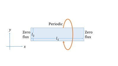
Figure 2: Domain on which the reaction diffusion model was solved with boundary conditions shown.

The shape of the domain was approximated based on the dimensions of C. elegans, where the length of the domain $l_{1}$ represents the length of the worm and the height of the domain $l_{2}$ represents the circumference of the worm. Since we are working in nondimensional coordinates where the characteristic length $L$ is equal to the length of the worm, $l_{1}=1.$ In C. elegans the length to maximum diameter ratio is approximately 18 [13]. Thus we set $l_{2}=0.2l_{1}$. The following boundary conditions are imposed on the domain ($\mathbf{W}=[u-u_{0},v-v_{0}]$):

$$\frac{d\mathbf{W}}{dx}_{x=0,l_{1}} =0$$

$$\frac{d\mathbf{W}}{dy}_{y=0} =-\frac{d\mathbf{W}}{dy}_{y=l_{2}}.$$

Periodic boundary conditions in the $y$ direction are used to approximate diffusion on a 2D cylindrical surface. Using these boundary conditions, the solutions to the linear problem take the form

$$\mathbf{w}(x,y,t)=\sum_{k}c_{k}e^{\lambda t}\mathbf{W}_{k}(x,y)$$ (13)

where the time independent eigenfunctions are

$$\textbf{W}_{k}(x,y)=\textbf{B}\cos\left(\frac{n\pi}{l_{1}}x\right)\left(\textbf{C}\sin\left(\frac{2m\pi}{l_{2}}y\right)+\textbf{D}\cos\left(\frac{2m\pi}{l_{2}}y\right)\right)$$ (14)

and the wavenumber $k$ is given by

$$k^{2}=\left(\frac{n\pi}{p}\right)^{2}+\left(\frac{2m\pi}{q}\right)^{2}.$$ (15)

Here $\lambda$ is the eigenvalue that determines the temporal growth of the modes and it is given by the roots of

$$\lambda^{2}+\lambda(k^{2}(1+d)-\gamma(f_{u}+g_{v}))+dk^{4}-\gamma(df_{u}-g_{v})k^{2}+\gamma^{2}(f_{u}g_{v}-f_{v}g_{u})=0$$ (16)

(see [25] for details). The partial derivatives of $f$ and $g$ are calculated at the steady state values of the system $(u_{0},v_{0})$. The expression $\lambda(k^{2})$ will be referred to as the dispersion relation. Modes with $\lambda(k^{2})>0$ grow as time increases, and represent the possible patterns that can be produced.

We used the CountourPlot3D and RegionPlot3D functions in Mathematica to numerically identify regions of parameter space that can lead to pattern formation [39]. These functions initially evaluate the criteria for pattern formation on a 3D grid and then uses an adaptive algorithm to evaluate the function on select subdivided regions to obtain the regions where the specified criteria are met. We generated two sets of region plots. First we examined which reaction parameters satisfied the Routh-Horwitz criterion. Then we incorporated spatial properties, including diffusion and domain size, to determine how these properties affect the number of possible modes that can result.

2.2 Data Analysis

We compared our model output to data on hsp-16.2 transcription in C. elegans [22]. This previous study obtained relative hsp-16.2 transcription levels in each of the 20 intestinal cells for 28 worms. Expression was measured 24 hours after heat shock using a C. elegans strain that contained a hsp-16.2 promoter bound to a gene for green fluorescent-protein (GFP). Thus, GFP fluorescence measured in live worms using microscopy serves as a marker for hsp-16.2 transcription.

To analyze the available data, we first averaged the GFP signal in cells within the same intestinal cell ring. There are a total of 9 intestinal cell rings in the C. elegans intestine; 4 cells in the anterior most cell ring and 2 cells in all the other cell rings. Cells within the same cell ring are at approximately the same distance down the length of the worm. Since our analysis predicts that variations in HSP production are only observed along the length of the worm and not along the circumference of the worm (see Section 3.1), we assume the rate of hsp-16.2 transcription is the same for cells within a single ring. Next, we used a rolling window to average across cell rings and smooth the data. For interior cell rings, the window length was three. For example, the value at the 4th cell ring was averaged with the 3rd and 5th to obtain an updated value at the 4th cell ring. For the edge cell rings we averaged the value of that cell ring with its one neighbor. Finally we normalized the data for each worm by dividing by the mean hsp-16.2 transcription value across all intestinal cells. This analysis resulted in nine spatial data points for each worm.

In order to compare this data to predictions from the mathematical model, we decomposed the data into the relevant trigonometric modes. Due to the zero flux boundary conditions of the system, we used only cosine modes for the analysis (see Equation 14). Here, again we assume that $m=0$ and thus the system reduces to a one dimensional problem. The nine normalized data points obtained for each worm lead to the inclusion of nine modes in the projection analysis. The contribution of each mode, $n=0,1,2,...,8$, is given as

$$p_{n}(x)=\alpha_{n}\cos\left(\frac{n\pi(x-1)}{8}\right)$$ (17)

where the expansion coefficients, $\alpha_{n},$ are

$$\alpha_{n}=\frac{1}{16}(y_{1}+\cos\left(n\pi\right)y_{9})+\frac{1}{8}\sum_{i=2}^{8}\cos\left(\frac{n\pi(i-1)}{8}\right)y_{i}\quad\quad n=0,8,$$ (18)

$$\alpha_{n}=\frac{1}{8}(y_{1}+\cos\left(n\pi\right)y_{9})+\frac{1}{4}\sum_{i=2}^{8}\cos\left(\frac{n\pi(i-1)}{8}\right)y_{i},\quad\quad n=1,2,..,7.$$ (19)

Here $y_{i}$ represents the normalized data from the $i$th intestinal cell ring. Using the expansion coefficients obtained for each worm, we grouped the worms using a k-means clustering analysis. We assessed the validity of this clustering approach using a bootstrap analysis as implemented in Flexible Procedures for Clustering package in R [12].

2.3 Model simulations

To examine how patterns form and what modes dominate with time, we simulated the reaction diffusion model using R v3.2.3 [30]. The PDE was simulated over a 2D grid using a finite difference approach as implemented in ReacTran (v1.3.2) [33]. The grid over which the system was solved was 100x20 cells. This resolution corresponds to an approximate resolution of 10 $\mu m$ which is much smaller than the length of an intestinal cell (approximately 100 $\mu m$) but much larger than the size of a protein. To perform simulations we used one of two initial conditions. In Case I the domain was initialized using the homogeneous steady state values for each ILP class and Gaussian noise was added. Specifically, each grid cell was initialized with the following dimensionless quantity of the two classes of ILPs

$$u_{ij} =u_{0}+\epsilon_{u,ij}$$

$$v_{ij} =v_{0}+\epsilon_{v,ij}$$

where $\epsilon_{u,ij}$ and $\epsilon_{v,ij}$ were drawn from normal probability distributions with means at $u_{0}$ and $v_{0}$ and standard deviations of $0.10u_{0}$ and $0.10v_{0}$, respectively. This level of variance was chosen to allow us to explore the effect of noise on the evolution of the system when it is perturbed from the homogeneous steady state. The initialization method avoids assumptions about where the pattern is initialized.

In Case II for model initialization, we explore our hypothesis that the heat shock response is initialized by an ILP stimulus at the head of the worm. Here, ILPs are added to one edge of the domain, corresponding to a release at the head of the worm. In this case the first column of the grid was initialized with the reaction steady-state values and the rest of the grid had no ILPs. Specifically, if $u_{ij}$, $v_{ij}$, represent the initial concentration of $u$, $v$, in grid cell $(i,j)$, for i=1,2,…,20 the initialization concentrations are given as

$$u_{i1} =u_{0}$$

$$v_{i1} =v_{0}$$

$$u_{ij} =0\quad\quad\quad j=2,3,...,100$$

$$v_{ij} =0\quad\quad\quad j=2,3,...,100.$$

Each simulation was run for for a dimensionless time $t^{*}$ of 2.0. We chose this value of $t^{*}$ because it represents the same time scale as the experimental data from [22]. Specifically, we have that $t^{*}=tD_{A}/L^{2}$, and we estimate that the length of the worm $L=1000$$\mu m$ and the diffusion rate $D_{A}$ is between 10 and 100 $\mu m^{2}/s$, i.e., the diffusion rate is between that of a protein in water and that of a protein in a cell [23]. This corresponds to a time between 12 hours and 6 days, which is on the same time scale as the data from the experiment which was obtained 24 hours post heat shock. When determining the steady-state of the system, in some cases it was necessary to run the simulation for a dimensionless time $t^{*}$of 3.0.

The source code for all the analyses perform is available on GitHub

3 Results

3.1 Reaction diffusion model predicts patterns along the length of the worm

The developed reaction diffusion model is capable of generating patterns reminiscent of intestinal hsp-16.2 expression patterns in C. elegans. The model has a total of 9 dimensionless parameters (Table 1).

Table 1: Parameters of the mathematical model. Values shown were used to perform model simulations. The justification for these parameter values is provided in the text.

Parameter	Value	Description
$a$	1	Relative inhibitory effect of DAF-16 on activator based on maximum production rate. The value implies activator production is completely controlled by DAF-16.
$b$	1	Relative inhibitory effect of DAF-16 on inhibitor based on maximum production rate. The value implies inhibitor production is completely controlled by DAF-16.
$c$	1	Relative decay rate of inhibitor to activator. The value implies the decay rate of the two classes of ILPs is the same.
$h$	0.4	Concentration of $p$ at which the feedback strength is half maximized. A low value implies feedback is very sensitive.
$r$	10	Hill coefficient describing feedback strength. The large value implies cooperativity exists in the system.
$k_{D,A}$	0.01	Dimensionless dissociation constant for the activator.
$k_{D,B}$	0.01	Dimensionless dissociation constant for the inhibitor.
$\gamma$	80	Relative domain size. Reasonable biological values lie between 0.01 and 100 (see text).
$d$	5	Ratio of diffusion rates between the two ILP classes. Implies the inhibitor diffuses 5 times as fast as the activator

In order to explore the model’s properties, where possible we set parameter values equal to biologically reasonable values. The parameters $a$ and $b$ were set equal to 1.0, implying that the expression of ILPs is completely under the control of DAF-16. That is, as $p$ approaches infinity, all DAF-16 is blocked from entering the nucleus and the net ILP production rate approaches zero. The parameter $c$ was set equal to one under the assumption that the two classes of ILPs decay at the same rate (i.e., $k_{3}=k_{6}$). For the remaining four parameters that describe the reactions in the system ($h$, $r$, $k_{D,A}$, and $k_{D,B}$) we sought to find biologically reasonable parameter values that together could result in diffusion driven instability.

We determined the range of biologically feasible values for $k_{D,A}$ and $k_{D,B}$ by first determining ranges for the values of the dissociation constants ($K_{D,A},$ $K_{D,B})$, ILP production rates ($k_{1},$ $k_{4}$), and ILP degradation rates ($k_{3}$) as follows. In humans, insulin likely binds to its receptor in two stages, leading to two dissociation constants of approximately 40 and 170 nM [34]. In our model we assume a single binding stage for all ILPs in C. elegans where the dissociation constant lies at a similar value (i.e. between 40 and 170 nM). The degradation half-life of proteins can vary drastically from 10 minutes to several days [4, 5]. This leads to degradation rates that vary between $10^{-6}$ s^-1 and $10^{-3}$ s^-1. As for production rates, the maximum protein production rate in E. coli ranges from 1 to $10^{6}$ molecules per generation, where the generation time is 21.5 minutes [18]. To translate the production rate units from molecules to molarity, we used a pseudocoelom volume range of 40 - 80 pL [3]. Putting this all together, we estimated that $k_{D,A}$ and $k_{D,B}$ values are likely between $10^{-3}$ and $10^{7}.$ This large range is primarily due to the uncertainty in ILP production and degradation rates. However, in subsequent sections, by using the mathematical model and the requirements for pattern formation we were able to further restrict this range.

Biological ranges for the values of $h$ and $r$ are more elusive. The value of $h$ depends on $H,$ $V_{max},$ and the degradation rate $k_{7}$. Both $H$ and $r$ are challenging to estimate since they describe the effect of DAF-2 activation on DAF-16 nuclear translocation, and the kinetics of this pathway have not been experimentally examined. Thus, to explore the pattern formation space we set a lower bound on $h$ of 0.05 but note that $h$ could potentially take on smaller values. Furthermore, the largest value of $r$ we explore is 10, but again this is not a biologically strict upper bound.

To have a diffusion driven instability the parameter values must satisfy the following Routh-Hurwitz stability criterion

$$f_{u}+g_{v} <0$$

$$f_{u}g_{v}-g_{u}f_{v} >0.$$ (20)

For diffusion to destabilize this system, $df_{u}+g_{v}>0.$ These inequalities imply that that either $f_{u}<0<g_{v}$ or $g_{v}<0<f_{u}$. We found these criteria were satisfied when $k_{D,A}<2$, $k_{D,B}>10$, and $r>1$ (Figure 3).

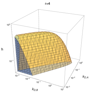
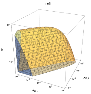
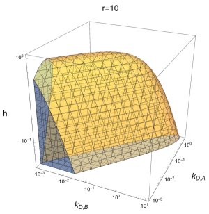
Figure 3: Parameter regions that satisfy the reaction requirements for diffusion driven instability. The area inside the surfaces represent the parameter space where diffusion driven instability can occur.

When performing the grid search with adaptive refinements, we set the minimum value of $k_{D,A}$ and $k_{D,B}$ equal to 0.001, the biological constraint obtained previously. We used integer values for $r$ of 1, 2, 4, 6, 8, and 10. At $r=1$, there were no regions that led to diffusion driven instability.

Although the constraints given by Equation 20 are necessary for pattern formation, they are not sufficient. Whether patterns can form and the number of possible modes also depends on the size of the domain and the difference in diffusion rates between the two classes of ILPs. For our purposes, the parameter $\gamma$ determines the size of the domain while $d$ gives the ratio of diffusion rates. An estimate for $\gamma$ depends on the characteristic length $L$ of the domain, the diffusion coefficient $D_{A},$ and the rate of ILP degradation $k_{3}$ together determine the value of $\gamma$. As discussed previously the protein degradation rate and diffusion rates are likely between $10^{-3}$ and $10^{-6}$ $s^{-1}$ and 10 - 100 $\mu m^{2}$/s, respectively [4, 5, 23]. The characteristic length is equivalent to the length of the worm, or 1.0 mm. This leads to possible values of $\gamma$ ranging from 0.01 to 100. Furthermore, we set a lower bound on the parameter $d$ based on the requirement that, for diffusion driven instability to occur, $d$ must be greater than the critical diffusion value $d_{c}$ given by the roots of following equation (see [25] for derivation):

$$d_{c}^{2}f_{u}^{2}+2(2f_{v}g_{u}-f_{u}g_{v})d_{c}+g_{v}^{2}=0.$$ (21)

For the example parameter set given (Table 1), the critical diffusion value $d_{c}$ is 2.97, implying the inhibitor class $B$ must diffuse at least 3 times faster than the activator class $A$.

We calculated the dispersion relation (Equation 16) as a function of $\gamma$ at different values of $d$ to determine how $\gamma$ and $d$ affect the number of possible modes (Figure 4).

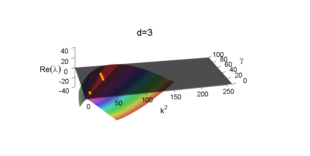
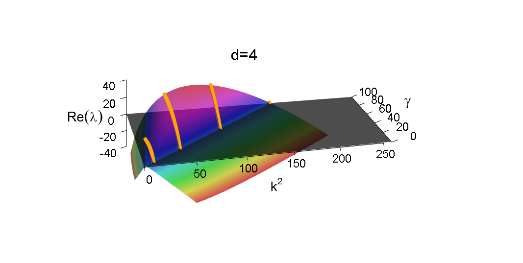
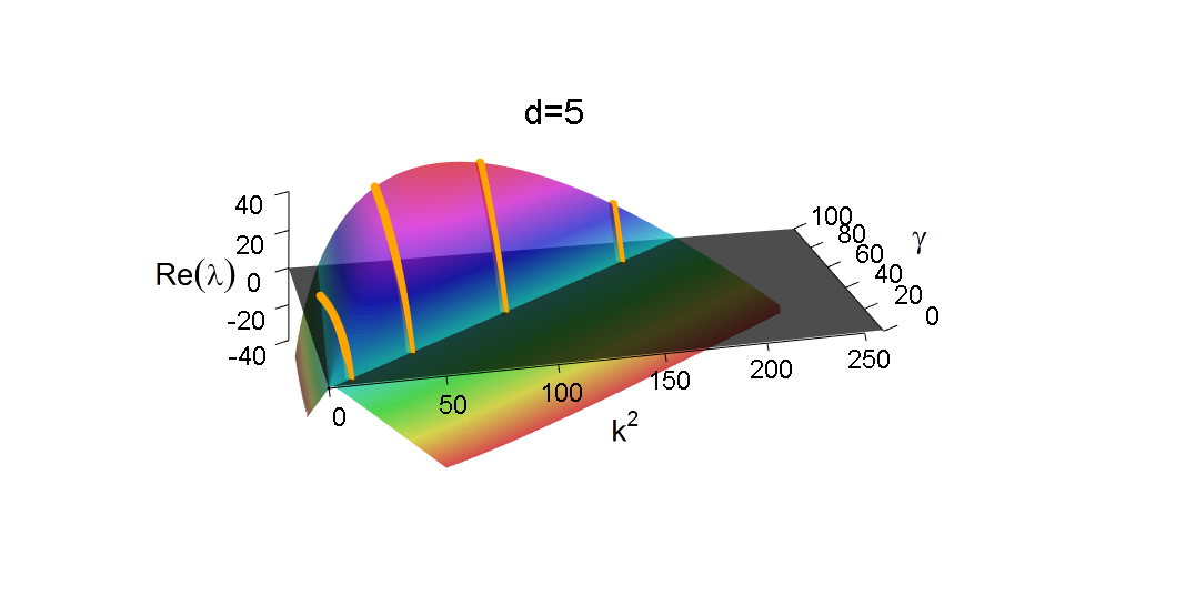
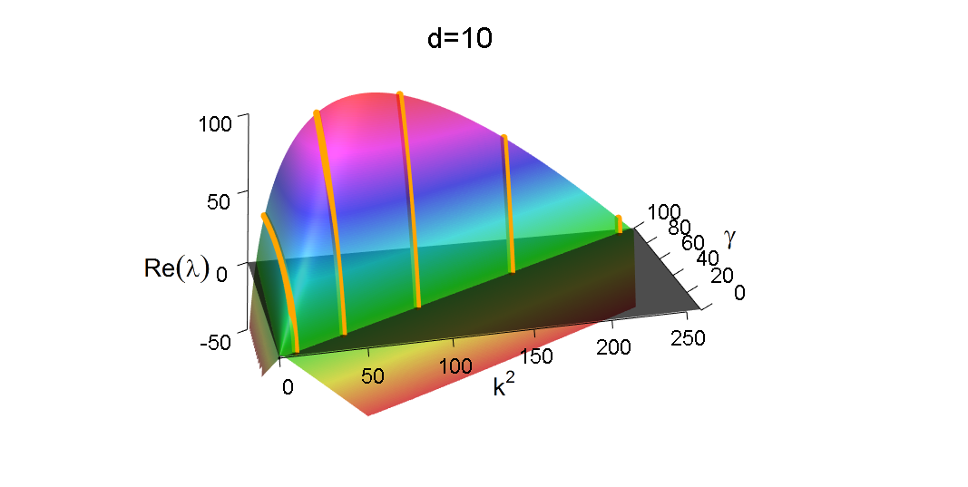
(a)

(b)

Figure 4: The dispersion relation reveals that more modes are possible given larger values of $\gamma$ and $d$. (a) The regions of the dispersion relation curve (Equation 16) with positive values of $Re(\lambda)$ represent the possible wavenumber $k^{2}$ under which modes can grow. Due to finite domain constraints only a discrete set of modes are possible, corresponding to discrete values of $k^{2}$ (Equation 15), shown with the yellow lines in each figure. Each yellow line represents a different mode, which from left to right correspond with $n=1,2,3,4,5$. (b) Visualization of the five different possible modes with the lowest mode ($n=1)$ on top and the highest mode ($n=5$) on bottom.

For this calculation all other parameter values were obtained from Table 1. Larger values of $\gamma$ and $d$ lead to a greater number of possible modes. In total when $d\leq 10$ and $\gamma\leq 100$, one of five modes can arise (Figure 4). These modes correspond to setting $n=1,2,3,4,5$ and $m=0$ in Equation 14. For larger values of $\gamma$ the first mode ($n=1$) eventually is no longer possible. In this analysis we found that, when setting $d\leq 10$ and $\gamma\leq 100$, there were no modes possible in which $m>0$. This implies that fluctuations in the HSP expression only occur along the length of the worm and not along the circumference of the worm.

To determine the dimensionless dissociation constants with more precision, we examined which parameter values resulted in patterned modes and how many modes were possible. We did this by using the parameters given in Table 1 but varied $r$, $k_{D,A}$, $k_{D,B}$, and $h$ to determine the number of possible stable modes as a function of the parameter values (Figure 5).

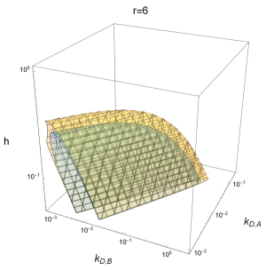
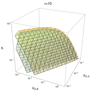
Figure 5: Total number of possible modes as a function of parameter values. In the larger orange shaded region only one mode is possible and in the smaller blue shaded region at least two modes are possible.

Given the constraints on the parameter values specified previously, to obtain at least one pattern formation mode $k_{D,A}$ must be less than 0.2, and $k_{D,B}$ must be less than 2.5 and $h$ must be less than 1. The parameter values become further constricted when we require that the system have at least two modes that grow with time.

3.2 Worms fall into two distinct groups based on HSP expression

To determine if the modes resulting from the hypothesized diffusion driven instability can explain experimental data on HSP expression patterns in C. elegans, we performed a clustering analysis. Worms were grouped using the expansion coefficients obtained from projecting trigonometric modes onto the data (Figure 6a).

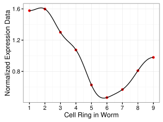
(a)

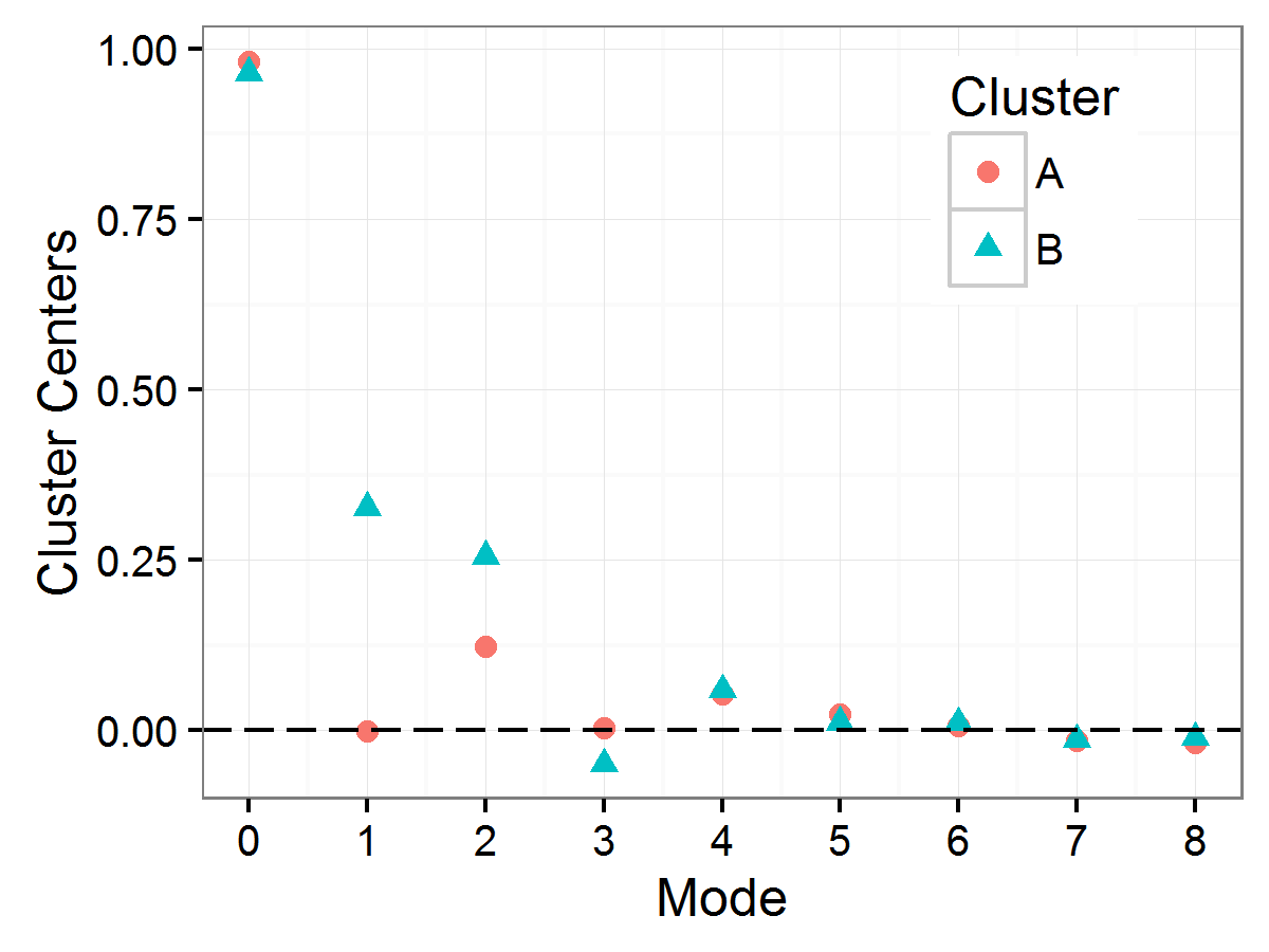
(b)

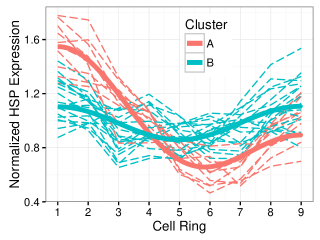
(c)

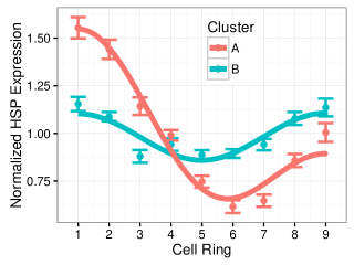
(d)

Figure 6: Clustering analysis reveals two distinct groups of worms. (a) Example individual worm data with interpolation using cosine modes weighted by expansion coefficients. (b) Cluster centers following a k[means analysis where clustering was done using the expansion coefficients for each cosine mode. (c) Individual worm data (thin dashed lines) compared with predicted profiles (thick solid lines) using summation of the dominate modes ($n$ = 0, 1 and 2 for Cluster A; $n$ = 0 and 2 for Cluster B). (d) Same as (c) but now showing the mean and standard error of the individual worm data.

This analysis reveals that C. elegans fall into two distinct groups based on HSP expression patterns. Using bootstrap methods, we found that grouping the worms into two clusters had strong support with mean Jaccard similarity scores of 0.92 and 0.89. However, when the number of groups was increased to three, this support decreased to 0.51, 0.79, and 0.60 for the three clusters.

Using the two cluster approach, we determined the dominate modes for each cluster (Figure 6b). Clearly the $n=0$ mode contributes significantly since this represents the averaged signal. For Cluster A the first and second mode also appear to have large contributions, and for Cluster B the second mode appears to have a large contribution. To determine if these specified modes are sufficient to explain the data, we overlayed the predicted spatial profiles using only these modes onto the the individual worm data (Figure 6c) and the mean worm data (Figure 6d). The predicted profiles using only the the specified dominate modes demonstrate a good match with the data.

3.3 Pattern formation in the Simulations

Our previous analysis reveals that a linearized version of the mathematical model produces stable oscillatory solutions. This result, however, does not guarantee that patterns will emerge from the full nonlinear model. Accordingly, we generated computational simulations of the nonlinear system. This allowed us to both check the validity of our analysis and verify that the model can reproduce the data on hsp-16.2 transcription in C. elegans. We performed a series of computational simulations of the full PDE system where we varied the values of $\gamma$ and $d$ and kept other parameter values constant (see Table 1 for values used). These simulations provide evidence supporting the existence of stable patterns, where the steady state is represented by a single dominate mode. We next compared these results to the clustering analysis presented previously. The model provides an explanation for how the pattern of a single dominate mode observed in Cluster B emerges (see Figure 6). However, the steady-state results do not explain the pattern of two equally dominate modes observed in Cluster A. We hypothesize that Cluster A is in a quasi-steady state where two modes are competing for dominance.

To determine if a quasi-steady state is possible, we examined whether we can predict the transition from a first mode dominate to a second mode dominate state based on the parameter values. In turn, we predict a quasi-steady state representing a combination of the first two modes may exist near this transition region. While our analysis of the linearized model predicts that several modes could exist, it does not predict which mode will dominate. There are analytical tools to perform such predictions and, for low-dimensional modes, they typically yield that the dominant mode will be the fastest growing mode or the mode for which $Re(\lambda)$ is maximized [25]. To see if this method could be used to predict the transition point from a first mode to a second mode dominate state, we compared the fastest growing mode to simulation results for the steady state (Figure 7).

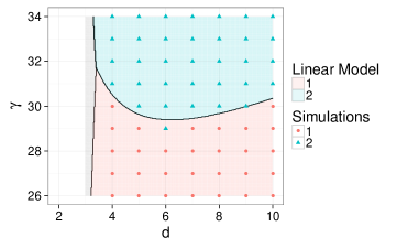
(a)

(b)

Figure 7: Comparison of the steady states obtained in simulations with predictions from the linearized model. (a) and (b) represent sets of simulations ran using two different initializations of Gaussian noise around the steady state. Each dot represents a single simulation of the full non-linear model and the color of the dot represents the dominate mode that the system eventually enters. The shaded regions represent the fastest growing mode as predicted by the linearized model. The linear model prediction roughly matches the dominate mode obtained using simulations of the full non linear model. However, the exact transition point from a first mode to second mode dominance depends on the initial conditions.

When the model is initialized using random noise around the steady-state for the reactions, we are able to roughly predict the transition region as a function of $\gamma$ and $d$. However, the exact transition point is sensitive to the initial conditions of the simulation.

To further explore this result we performed simulations at points in parameter space near the transition region. Specifically, we set $\gamma=30$.2 and $d=5$. At this point, simulations initialized using Gaussian noise around the steady-state showed that the second mode is dominate. We found with this parameter combination that the system sometimes enters a quasi-steady state (Figure 8 and 9).

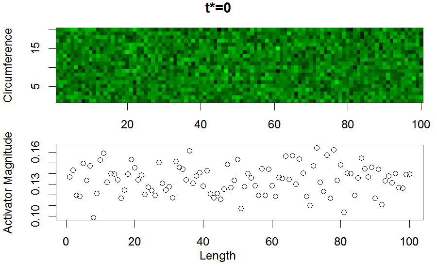
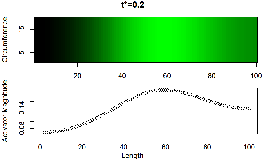
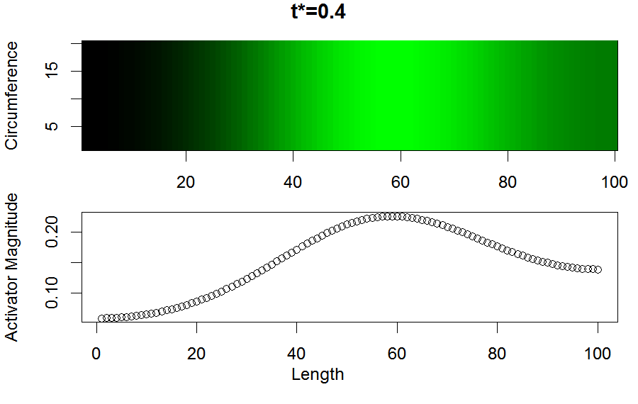
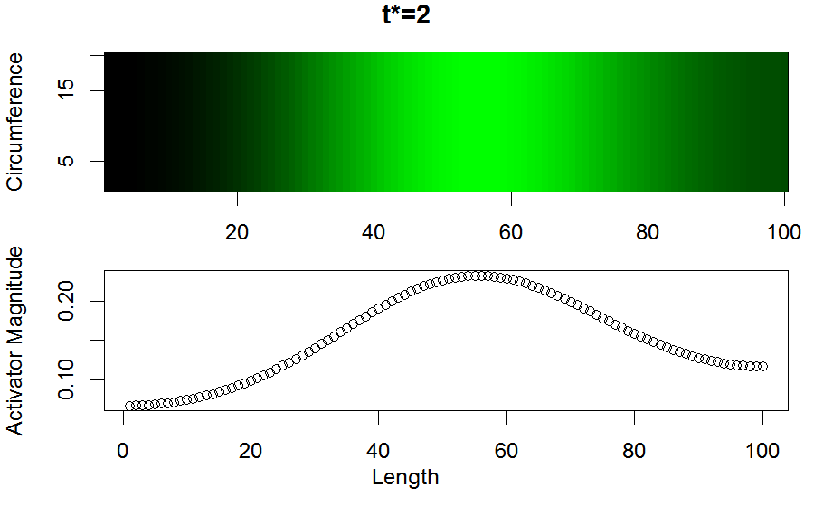
Figure 8: Simulation initialized with Gaussian noise that enters a quasi-steady state. Showing simulation results at four different values of $t^{*}$. The activator magnitude shown represents the top horizontal line shown in the domain.

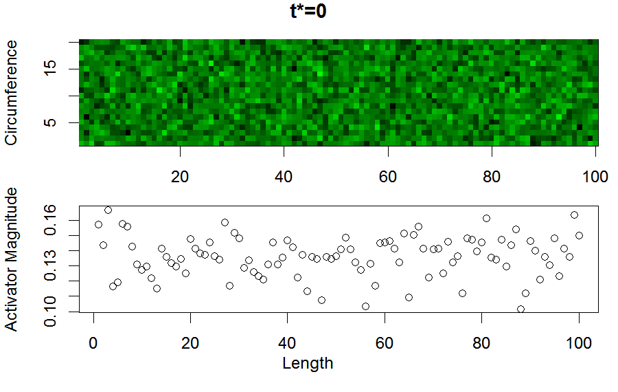
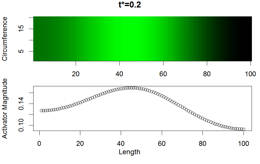
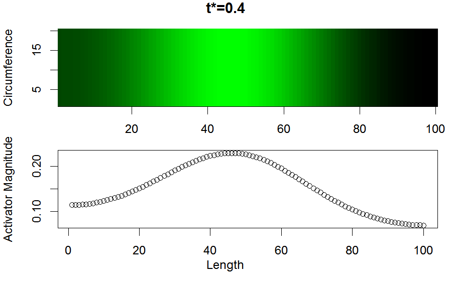
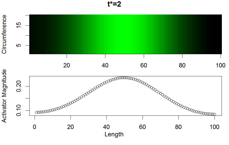
Figure 9: Simulation initialized with Gaussian noise that has entered a steady-state mode by $t^{*}=2$. Showing simulation results at four different values of $t^{*}.$ The activator magnitude shown represents the top horizontal line shown in the domain.

However, the progression into this state is sensitive to the specific Gaussian noise present in the initialization. For example, in one initialization the system appears to still be in a quasi-steady state at $t^{*}=2.0$ (Figure 8), while in a second initialization the system has entered the steady state at $t^{*}=2.0$ (Figure 9).

We next performed simulations where the pattern was initialized at the left end of the domain. Biologically this corresponds to a release of ILPs at the anterior region of the worm’s intestine. We found that at multiple values of $\gamma$ and $d$ the observed pattern orientation was accurately reproduced (an example is shown in Figure 10).

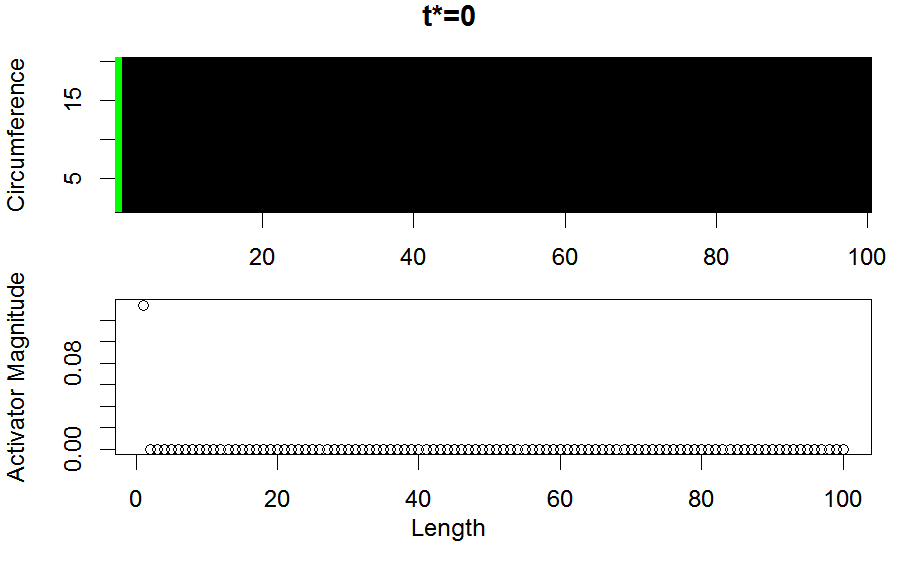
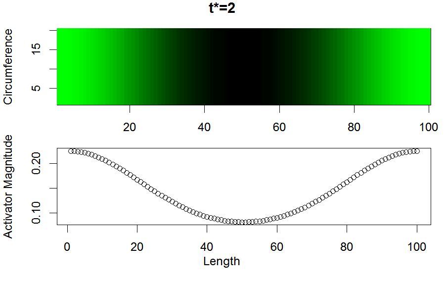
Figure 10: Results of simulation initialized using left constant conditions. (Left) Condition used to initialize simulation. (Right) Simulation results where $\gamma=37$ and $d=4$. All other parameters are given in Table 1. The activator magnitude shown represents the top horizontal line shown in the domain.

The simulation predicts increased hsp-16.2 transcription at the head and the tail of the worm and this matches what is observed experimentally. This is in contrast to the simulations initialized using Gaussian noise across the domain (Figure 8 and 9). These simulations predict reflected versions of the pattern may arise (i.e., decreased transcription of hsp-16.2 at either end of the domain compared with the middle). Thus, the initial conditions may explain why only one orientation of mode 1 and 2 are observed experimentally.

4 Discussion

We developed a reaction diffusion model that predicts experimentally observed patterns in the transcription of hsp-16.2, a biomarker of aging [22, 31]. This work provides insight into the mechanism of the non-cell autonomous heat shock response in the nematode C. elegans. We hypothesized that the transcription of hsp-16.2 is dependent on a complex interplay of insulin like peptides signaling at a multicellular level. This complex system warrants the use of mathematical tools to understand how changes in the system affect the total levels of hsp-16.2 transcription. Furthermore, since hsp-16.2 transcription is correlated with lifespan, the development of a mathematical model that connects thermal injury to intestinal hsp-16.2 transcription allows us to study how alterations to kinetic or diffusive parameters in this system might be related to aging.

We derived constraints on the values of four parameters in the system by combining biological intuition with the requirement for diffusion driven instability. To obtain patterns, the reaction parameters must satisfy the Routh-Horwitz conditions. Furthermore, parameter values are constrained by the spatial and diffusive properties of the system, including the difference in the diffusion rate between the two classes of ILPs and the domain size. Ultimately, when setting the minimum value of $h$ to 0.05, and the maximum value of $r$ to 10, to obtain patterned modes $k_{D,A}$ must be between 0.001 and 0.2 while $k_{D,B}$ must be between 0.001 and 2.5 (see Table 1 for the values of other parameters). These dimensionless dissociation constants are equal to the actual dissociation constant multiplied by the ILP decay/production ratio ($k_{3}/k_{1}$, $k_{3}/k_{4}$). Although the actual dissociation constants for the DAF-2 agonists and antagonists are currently unknown, they are likely on the order of 10-100 nM [34], leading to an ILP decay/production ratio range of $10^{-5}$ to $10^{-1}$ $nM^{-1}.$We also obtained parameter constraints related to the feedback strength in the system. The parameter $h$ represents the strength of the feedback; as $h$ increases more stimulus is required for the same response size. Thus, an upper bound on the value of $h$ of 1.0 implies that a minimal feedback strength is required for pattern formation to occur. We found no lower bound on the value of $h$, suggesting that there is not a maximal feedback strength. The Hill coefficient $r$, which determines the sharpness of the feedback response must be greater than one, suggesting some cooperativity in the system may exist. There are several signaling motifs that could lead to a Hill coefficient greater than one [40]. One such process involves non-processive multisite protein phosphorylation by a single kinase. The nuclear translocation of DAF-16 is potentially blocked when DAF-16 is phosphorylated by AKT at one or multiple sites [20]. Thus, it may be the requirement for multi-site phosphorylation of DAF-16 that leads to the large Hill coefficient predicted by the model.

To derive these parameter constraints, the values of three other parameters were set to constant values. By setting $a$ and $b$ equal to one, we assumed ILP transcription was completely dependent on DAF-16 nuclear localization. However, this is likely not the case since there could be other transcription factors that affect ILP transcription. If $a$ and $b$ were less than one, this would imply that there is a baseline level of ILP production without DAF-16 nuclear localization. Values of $a$ and $b$ greater than one are not biologically possible, since this would lead to negative production rates. The third parameter value $c$ was set equal to one, implying that the two classes of ILPs decay at the same rate. This is an assumption that warrants future investigation. Very little is currently known about ILP degradation in C. elegans. In higher level organisms, such as rats and humans, insulin is typically endocytosed by cells with insulin-receptors and is degraded within the cells [2, 6]. These processes likely depend on specific properties of the insulin-like peptides such as specific and non-specific binding affinities that determine the likelihood of endocytosis and subsequent degradation.

The model presented here provides a mechanistic explanation for the data obtained on hsp-16.2 expression patterns in C. elegans. A previous study found that hsp-16.2 transcription in intestinal cells was greatest in the anterior region, followed by the posterior region, and finally least in the middle of the worm [22]. We sought to use the developed model to provide an explanation for this spatial profile. Since the mean spatial profile of the 28 worms studied did not clearly match one of the modes predicted by the model, we hypothesized that the worms fell into multiple groups with different expression patterns. Using a clustering analysis, we found that the worms could be divided into two groups. One of these groups had a clear single dominate mode; however, the second group had two modes that contributed equally to the spatial profile. Due to a lack of bootstrap support, we did not attempt to divide the worms up into more than two groups.

The cluster with two dominate modes may represent worms that have not yet reached a steady state in their hsp-16.2 transcription spatial profiles. To explore this possibility we performed simulations to determine if the system could get temporarily stuck in a state between the first two modes. We found that a reasonable method for predicting whether the first or second mode would dominate is to determine what mode grows the fastest according to the linearized model. We predicted that if two modes grow at a roughly equal pace, then the system may reside in a quasi-steady state that represents a superpositioning of the two modes. In our simulations we found that this was indeed the case (Figure 8 and 9); however, the dynamics of the system ultimately depended on the initial conditions. This dependency could explain why some worms appear to have reached a steady state 24 hours after heat shock and other worms have not.

The mathematical model presented demonstrates how patterns can emerge but represents a simplification of the actual signaling pathways within C. elegans. There are over 40 ILPs that have been identified in C. elegans, and the action of each ILP does not necessary fit precisely into one of the two classes of ILPs included in the model. For instance, in the model DAF-16 only has a stimulatory effect on the production of ILPs. In reality, DAF-16 increases the production of some ILPs and decreases the production of others. This leads to ILP agonists that are both self-activating (e.g., INS-7) and self-inhibiting (e.g., INS-6) [15, 24]. This is in contrast to our model where, we treat the ILP class that agonizes DAF-2 as purely self-inhibiting. The model is meant to capture the net effect of DAF-16 on all ILP agonists, and, thus, we do not include ILP agonists that are both activated and inhibited by DAF-16. We did however explore a model where the dimensionless parameter $b$ is negative, implying DAF-16 has a net inhibitory effect on ILP agonists. We were able to show that when $b$ is less than zero it is not possible to satisfy the requirements for diffusion driven instability (see Appendix A). Given this result we propose that although INS-7 acts through a self-activating loop, there are other self-inhibiting DAF-2 agonists that counteract this effect.

Here, we present a specific mechanism to explain the patterns observed in hsp-16.2 expression, however other mechanisms may contribute to the observed patterns. We propose that serotonin at the head of the worm leads to the release of ILPs that then diffuse through the pseudocoelom of the worm. This is based on two key experimental findings: (1) thermal injury leads to the release of serotonin from neurons at the head of the worm and this release is essential for the heat shock response in intestinal cells [35, 28]; (2) the DAF-2 insulin like receptor is key for the heat shock response to be activated in intestinal cells [19]. Thus, there must be a link between serotonin and the insulin-like signaling pathway. In an alternate mechanism, serotonin may stimulate other neurons and lead to a signal propagation through the peripheral nervous system. However, the intestine in C. elegans is not directly innervated [1], so a diffusive process is still essential. It is also possible that serotonin itself diffuses through the pseudocoelom and directly activates the heat shock response in intestinal cells. However, experiments have not yet revealed the presence of serotonin receptors on intestinal cells and this mechanism does not explain why DAF-2 is an essential component of the process. Finally, patterned HSP expression may be, in part, caused by coelomocytes in the pseudocoelom. Coelomocytes are large, endocytotic cells situated in relatively constant positions in the psuedocoelomic cavity [8]. Their endocytotic properties make it likely that they function similar to immune cells. There are 6 coelomocytes located within C. elegans, and one study has suggested that they may endocytose ILPs [17]. The six coelomocytes are located in pairs at the anterior, the mid body, and the posterior of the worm. If coelomocytes endocytose a large amount of ILPs this would affect the ILP concentration in a spatially dependent manner and result in cell to cell variation in the level of DAF-2 activation. Due to these potential alternate mechanisms, future work is needed to validate the mathematical model. For example, the model predicts that DAF-16 nuclear localization would occur in a patterned fashion, similar to the hsp-16.2 transcription patterns. Thus, an experiment measuring the localization of DAF-16 within individual intestinal cells would help validate the proposed mechanism.

Although the model provides an explanation for how patterns in protein expression arise, the initialization of these patterns is not explicitly included. We hypothesize that the patterning is initiated by a stimulus at the head of the worm. The data shows hsp-16.2 transcription is consistently higher in anterior and posterior intestinal cells compared with middle intestinal cells. However, given random initialization conditions, the model predicts that the reflected version of this pattern in which expression levels are minimized at the edges would also be observed. When performing simulations where ILPs were initially only present at the left end of the domain, we found the resulting pattern had an orientation that matched the data (Figure 10). This asymmetric initialization provides an explanation for why reflected versions of the pattern are never observed in the data. Finally, we note that as the model currently stands, ILP transcription will occur regardless of the initialization conditions. However, under healthy conditions this transcription should not occur. Thus, the model assumes the stressor has affected the system in some way as to allow for ILP transcription. Future work could involve exploring the nature of this alteration to the system. A deeper understanding of the initialization process could provide insight into how different magnitudes of hsp-16.2 arise.

It is not known whether hsp-16.2 transcription directly affects aging or if it is upstream events that are the driver of aging. In the latter case, the model allows us to predict what the upstream drivers may actually be. For instance, DAF-16 is a transcription factor that regulates the expression of many proteins besides ILPs. As such, DAF-16 nuclear translocation may play an important role in aging. We can use the model to assess how altered parameter values might affect the amount of DAF-16 nuclear localization. Alternatively, the model allows us to examine how known effects of aging might alter the system. Protein turnover dynamics are known to be affected during the aging process [38]. Thus, we can study how these effects might propagate through the system and potentially exacerbate the aging process. This work can be used to help understand how different magnitudes of hsp-16.2 expression arise and why higher levels of hsp-16.2 transcription are associated with aging.

5 Acknowledgments

JMW is supported in part by an NSF GRFP and in part by the Interdisciplinary Quantitative Biology (IQ Biology) program at the BioFrontiers Institute, University of Colorado, Boulder. IQ Biology is generously supported by NSF IGERT grant number 1144807. AM is supported by the National Institute on Aging at the National Institutes of Health by grant 4R00AG045341. The authors would also like to thank T. E. Johnson (University of Colorado, Boulder) for insightful discussions and suggestions concerning this work.

Appendix Appendix A Alternative Mechanism

Here we explore an alternate system in which the ILP class that acts as a DAF-2 agonist, $B$, is repressed by DAF-16 nuclear localization. This implies that $B$ regulates its own production through a positive feedback loop rather than through a negative feedback loop as presented in the main paper. The following system of equations describes this alternative model:

$$\frac{\partial A}{\partial t} =F(A,B)+D_{A}\nabla^{2}A$$ (22)

$$\frac{\partial B}{\partial t} =G(A,B)+D_{B}\nabla^{2}B$$ (23)

where

$$F(A,B)= k_{1}-k_{2}\frac{P^{r}}{H^{r}+P^{r}}-k_{3}A$$ (24)

$$G(A,B)= k_{4}+k_{5}\frac{P}{H^{r}+P^{r}}-k_{6}B$$ (25)

and

$$P=\frac{V_{max}B}{k_{7}(K_{m}(1+\frac{A}{K_{i}})+B)}.$$ (26)

The system was made dimensionless using the following substitutions

$$t^{*} =D_{A}t/L^{2} x^{*} =x/L d =D_{B}/D_{A}$$

$$\gamma =k_{3}L^{2}/D_{A} u =Ak_{3}/k_{1} v =Bk_{3}/k_{4}$$

$$p =Pk_{7}/V_{max} a =k_{2}/k_{1} b =k_{5}/k_{4}$$

$$c =k_{6}/k_{3} h =H(k_{7}/V_{max}) k_{D,A} =K_{D,A}k_{3}/k_{1}$$

$$k_{D,B} =K_{D,B}k_{3}/k_{4}$$

where all the parameters must take on positive values. This leads to the following system of equations

$$\frac{\partial u}{\partial t^{*}}=\gamma f(u,v)+\nabla^{2}u$$ (27)

$$\frac{\partial v}{\partial t^{*}}=\gamma g(u,v)+d\nabla^{2}u$$ (28)

where

$$f(u,v) =1-a\frac{p(u,v)^{r}}{h^{r}+p(u,v)^{r}}-u$$ (29)

$$g(u,v) =1+b\frac{p(u,v)^{r}}{h^{r}+p(u,v)^{r}}-cv.$$ (30)

$$p(u,v) =\frac{v}{k_{D,B}(1+\frac{u}{k_{D,A}})+v}$$ (31)

Ignoring diffusion and linearizing about the steady state ($u_{0},v_{0}$) leads to the following differential equation:

$$w_{t}=\gamma Aw,\quad w=\left[\begin{array}[]{l}u-u_{0}\\ v-v_{0}\end{array}\right],\quad A=\left[\begin{array}[]{ll}f_{u}&f_{v}\\ g_{u}&g_{v}\end{array}\right]_{(u_{0},v_{0})}.$$ (32)

For diffusion driven instability to occur, the system must be stable without diffusion, leading to the following requirements:

$$f_{u}+g_{v} <0$$ (33)

$$f_{u}g_{v}-g_{u}f_{v} >0.$$ (34)

The partial derivatives of $f(u,v)$ and $g(u,v)$ are

$$f_{u} =\frac{ah^{r}rk_{D,B}v^{r}}{k_{D,A}Z^{2}}Y-1$$ (35)

$$f_{v} =-\frac{arv^{r-1}}{Z}+\frac{av^{r}}{Z^{2}}(rv^{r-1}+h^{r}rY)$$ (36)

$$g_{u} =-\frac{bh^{r}rk_{D,B}v^{r}}{k_{D,A}Z^{2}}Y$$ (37)

$$g_{v} =\frac{brv^{r-1}}{Z}-\frac{bv^{r}}{Z^{2}}(rv^{r-1}+h^{r}rY)-c$$ (38)

where

$$Z =v^{r}+h^{r}(k_{D,B}(1+\frac{u}{k_{D,A}})+v)^{r}.$$ (39)

$$Y =(k_{D,B}(1+\frac{u}{k_{D,A}})+v)^{r-1}$$ (40)

Using the condition given by Equation 34 and a series of algebraic manipulations, we obtain the following inequalities that must hold for diffusion driven instability to occur

$$f_{u}g_{v}-g_{u}f_{v}>0\implies \left(\frac{ah^{r}rk_{D,B}v^{r}}{k_{D,A}Z^{2}}Y-1\right)\left(\frac{brv^{r-1}}{Z}-\frac{bv^{r}}{Z^{2}}(rv^{r-1}+h^{r}rY)-c\right)$$

$$-\left(-\frac{bh^{r}rk_{D,B}v^{r}}{k_{D,A}Z^{2}}Y\right)\left(-\frac{arv^{r-1}}{Z}+\frac{av^{r}}{Z^{2}}(rv^{r-1}+h^{r}rY)\right)>0$$ (41)

$$\implies -\frac{brv^{r-1}}{Z}+\frac{bv^{r}}{Z^{2}}(rv^{r-1}+h^{r}rY)-\left(\frac{ah^{r}rk_{D,B}v^{r}}{k_{D,A}Z^{2}}Y-1\right)c>0$$ (42)

$$\implies -Zbrv^{r-1}+bv^{r}(rv^{r-1}+h^{r}rY)-\frac{ah^{r}rk_{D,B}cv^{r}}{k_{D,A}}Y+cZ^{2}>0$$ (43)

$$\implies -\left(v^{r}+h^{r}\left(k_{D,B}\left(1+\frac{u}{k_{D,A}}\right)+v\right)^{r}\right)brv^{r-1}$$

$$+bv^{r}(rv^{r-1}+h^{r}rY)-\frac{ah^{r}rk_{D,B}v^{r}c}{k_{D,A}}Y+cZ^{2}>0$$ (44)

$$\implies -brv^{2r-1}-bh^{r}rv^{r-1}Y\left(k_{D,B}\left(1+\frac{u}{k_{D,A}}\right)+v\right)$$ (45)

$$+brv^{2r-1}+bh^{r}rv^{r}Y-\frac{ah^{r}rk_{D,B}cv^{r}}{k_{D,A}}Y+cZ^{2}>0$$ (46)

$$\implies -bh^{r}rv^{r-1}Y\left(k_{D,B}\left(1+\frac{u}{k_{D,A}}\right)+v\right)+bh^{r}rv^{r}Y-\frac{ah^{r}rk_{D,B}cv^{r}}{k_{D,A}}Y+cZ^{2}>0$$ (47)

$$\implies -bh^{r}rk_{D,B}v^{r-1}Y\left(1+\frac{u}{k_{D,A}}\right)-\frac{ah^{r}rk_{D,B}cv^{r}}{k_{D,A}}Y+cZ^{2}>0$$ (48)

Furthermore, for diffusion to cause instability in the system the following relation must hold

$$df_{u}+g_{v}>0.$$ (49)

Taken together with Equation 33, this implies that $f_{u}$ and $g_{v}$ must have opposite signs. This leads to two possible cases. In Case 1, $f_{u}>0$ and $g_{v}<0$, and in Case 2, $f_{u}<0$ and $g_{v}>0$. For Case 1, using Equations 35 and 38, we derive the following inequalities:

$$f_{u}>0\implies \frac{ah^{r}rk_{D,B}v^{r}}{k_{D,A}}\left(k_{D,B}\left(1+\frac{u}{k_{D,A}}\right)+v\right)^{r-1}>Z^{2}$$ (50)

$$g_{v}<0\implies cZ^{2}>Zbrv^{r-1}-bv^{r}\left(rv^{r-1}+h^{r}r\left(k_{D,B}\left(1+\frac{u}{k_{D,A}}\right)+v\right)^{r-1}\right)$$ (51)

$$\implies cZ^{2}>brv^{2r-1}+bh^{r}rv^{r-1}\left(k_{D,B}\left(1+\frac{u}{k_{D,A}}\right)+v\right)^{r}-brv^{2r-1}$$

$$-bh^{r}rv^{r}\left(k_{D,B}\left(1+\frac{u}{k_{D,A}}\right)+v\right)^{r-1}$$ (52)

$$\implies Z^{2}>\frac{bh^{r}rv^{r-1}}{c}\left(\left(k_{D,B}\left(1+\frac{u}{k_{D,A}}\right)+v\right)^{r}-v\left(k_{D,B}\left(1+\frac{u}{k_{D,A}}\right)+v\right)^{r-1}\right)$$ (53)

$$\implies Z^{2}>\frac{bh^{r}rv^{r-1}}{c}\left(k_{D,B}\left(1+\frac{u}{k_{D,A}}\right)+v\right)^{r-1}\left(\left(k_{D,B}\left(1+\frac{u}{k_{D,A}}\right)+v\right)-v\right)$$ (54)

$$\implies Z^{2}>\frac{bh^{r}rk_{D,B}v^{r-1}}{c}\left(k_{D,B}\left(1+\frac{u}{k_{D,A}}\right)+v\right)^{r-1}\left(1+\frac{u}{k_{D,A}}\right).$$ (55)

In summary, for Case 1, $Z^{2}$ must satisfy the following inequality (using Equation 40):

$$\frac{bh^{r}rk_{D,B}v^{r-1}}{c}\left(1+\frac{u}{k_{D,A}}\right)Y<Z^{2}<\frac{ah^{r}rk_{D,B}v^{r}}{k_{D,A}}Y.$$ (56)

Thus, for Case 1, using the fact that the determinate of $A$ must be greater than zero (Equation 48) and the upper bound on $Z^{2}$ given in Equation 56 we have that

$$\frac{ah^{r}rk_{D,B}v^{r}}{k_{D,A}}Y>Z^{2}>\frac{bh^{r}rk_{D,B}v^{r-1}}{c}(1+\frac{u}{k_{D,A}})Y+\frac{ah^{r}rk_{D,B}v^{r}}{k_{D,A}}Y$$ (57)

$$\implies 0>Z^{2}-\frac{ah^{r}rk_{D,B}v^{r}}{k_{D,A}}Y>\frac{bh^{r}rk_{D,B}v^{r-1}}{c}(1+\frac{u}{k_{D,A}})Y$$ . (58)

However, this inequality is not possible since all the parameter values are greater than zero.

A similar argument holds for Case 2. Using the same steps as shown in Equations 50 - 55, but reversing the equality sign, $Z^{2}$ must satisfy the following inequality:

$$\frac{ahrk_{D,B}v^{r}}{k_{D,A}}Y<Z^{2}<\frac{bhrk_{D,B}v^{r-1}}{c}\left(1+\frac{u}{k_{D,A}}\right)Y.$$ (59)

Equation 48 and 59 imply that

$$\frac{bhrk_{D,B}v^{r-1}}{c}\left(1+\frac{u}{k_{D,A}}\right)Y>Z^{2}>\frac{bhrk_{D,B}v^{r-1}}{c}\left(1+\frac{u}{k_{D,A}}\right)Y+\frac{ahrk_{D,B}v^{r}}{k_{D,A}}Y$$ (60)

$$\implies 0>Z^{2}-\frac{bhrk_{D,B}v^{r-1}}{c}\left(1+\frac{u}{k_{D,A}}\right)Y>\frac{ahrk_{D,B}v^{r}}{k_{D,A}}Y$$ . (61)

Since the parameters are positive, the final term in Equation 61 can not be less than zero. Thus, for this system it is not possible for the determinate of $A$ to be greater than zero and for $f_{u}$ and $g_{v}$ to have opposite signs. Therefore, diffusion driven instability cannot occur.

References

- Altun and Hall [2009] Altun, Z., Hall, D., 2009. Alimentary system, intestine. In: WormAtlas.
-
Bai and Chang [1995]
Bai, J. P., Chang, L. L., aug 1995. Transepithelial transport of insulin: I.
Insulin degradation by insulin-degrading enzyme in small intestinal
epithelium. Pharmaceutical research 12 (8), 1171–5.
URL http://www.ncbi.nlm.nih.gov/pubmed/7494830 -
Banse and Hunter [2012]
Banse, S. A., Hunter, C. P., mar 2012. Vampiric isolation of extracellular
fluid from Caenorhabditis elegans. Journal of visualized experiments :
JoVE (61).
URL http://www.ncbi.nlm.nih.gov/pubmed/22453516 -
Belle et al. [2006]
Belle, A., Tanay, A., Bitincka, L., Shamir, R., O’Shea, E. K., aug 2006.
Quantification of protein half-lives in the budding yeast proteome.
Proceedings of the National Academy of Sciences of the United States of
America 103 (35), 13004–9.
URL http://www.ncbi.nlm.nih.gov/pubmed/16916930 -
Cambridge et al. [2011]
Cambridge, S. B., Gnad, F., Nguyen, C., Bermejo, J. L., Krüger, M., Mann,
M., dec 2011. Systems-wide proteomic analysis in mammalian cells reveals
conserved, functional protein turnover. Journal of proteome research
10 (12), 5275–84.
URL http://www.ncbi.nlm.nih.gov/pubmed/22050367 -
Duckworth et al. [1998]
Duckworth, W. C., Bennett, R. G., Hamel, F. G., oct 1998. Insulin degradation:
progress and potential. Endocrine reviews 19 (5), 608–24.
URL http://www.ncbi.nlm.nih.gov/pubmed/9793760 -
Ewbank [2006]
Ewbank, J., 2006. Signaling in the immune response. WormBook.
URL http://www.wormbook.org/chapters/www{_}signalingimmuneresponse/signalingimmuneresponse.html -
Fares and Grant [2002]
Fares, H., Grant, B., jan 2002. Deciphering endocytosis in Caenorhabditis
elegans. Traffic (Copenhagen, Denmark) 3 (1), 11–9.
URL http://www.ncbi.nlm.nih.gov/pubmed/11872138 -
Hartwig et al. [2009]
Hartwig, K., Heidler, T., Moch, J., Daniel, H., Wenzel, U., mar 2009. Feeding
a ROS-generator to Caenorhabditis elegans leads to increased expression of
small heat shock protein HSP-16.2 and hormesis. Genes & nutrition 4 (1),
59–67.
URL http://www.ncbi.nlm.nih.gov/pubmed/19252938 -
Haslbeck et al. [2005]
Haslbeck, M., Franzmann, T., Weinfurtner, D., Buchner, J., oct 2005. Some like
it hot: the structure and function of small heat-shock proteins. Nature
structural & molecular biology 12 (10), 842–6.
URL http://www.ncbi.nlm.nih.gov/pubmed/16205709 -
Hasselman [2016]
Hasselman, B., 2016. nleqslv: Solve Systems of Nonlinear Equations.
URL https://cran.r-project.org/package=nleqslv -
Hennig [2015]
Hennig, C., 2015. fpc: Flexible Procedures for Clustering.
URL https://cran.r-project.org/package=fpc -
Hirose et al. [2003]
Hirose, T., Nakano, Y., Nagamatsu, Y., Misumi, T., Ohta, H., Ohshima, Y., mar
2003. Cyclic GMP-dependent protein kinase EGL-4 controls body size and
lifespan in C elegans. Development (Cambridge, England) 130 (6), 1089–99.
URL http://www.ncbi.nlm.nih.gov/pubmed/12571101 -
Hsu et al. [2003]
Hsu, A.-L., Murphy, C. T., Kenyon, C., may 2003. Regulation of aging and
age-related disease by DAF-16 and heat-shock factor. Science (New York,
N.Y.) 300 (5622), 1142–5.
URL http://www.ncbi.nlm.nih.gov/pubmed/12750521 -
Hua et al. [2003]
Hua, Q.-X., Nakagawa, S. H., Wilken, J., Ramos, R. R., Jia, W., Bass, J.,
Weiss, M. A., apr 2003. A divergent INS protein in Caenorhabditis elegans
structurally resembles human insulin and activates the human insulin
receptor. Genes & development 17 (7), 826–31.
URL http://www.ncbi.nlm.nih.gov/pubmed/12654724 -
Kaletsky et al. [2016]
Kaletsky, R., Lakhina, V., Arey, R., Williams, A., Landis, J., Ashraf, J.,
Murphy, C. T., jan 2016. The C. elegans adult neuronal IIS/FOXO
transcriptome reveals adult phenotype regulators. Nature 529 (7584), 92–6.
URL http://www.ncbi.nlm.nih.gov/pubmed/26675724 -
Kao et al. [2007]
Kao, G., Nordenson, C., Still, M., Rönnlund, A., Tuck, S., Naredi, P.,
feb 2007. ASNA-1 positively regulates insulin secretion in C. elegans and
mammalian cells. Cell 128 (3), 577–87.
URL http://www.ncbi.nlm.nih.gov/pubmed/17289575 -
Li et al. [2014]
Li, G.-W., Burkhardt, D., Gross, C., Weissman, J. S., apr 2014. Quantifying
absolute protein synthesis rates reveals principles underlying allocation of
cellular resources. Cell 157 (3), 624–35.
URL http://www.ncbi.nlm.nih.gov/pubmed/24766808 -
Liang et al. [2006]
Liang, B., Moussaif, M., Kuan, C.-J., Gargus, J. J., Sze, J. Y., dec 2006.
Serotonin targets the DAF-16/FOXO signaling pathway to modulate stress
responses. Cell metabolism 4 (6), 429–40.
URL http://www.ncbi.nlm.nih.gov/pubmed/17141627 -
Lin et al. [2001]
Lin, K., Hsin, H., Libina, N., Kenyon, C., jun 2001. Regulation of the
Caenorhabditis elegans longevity protein DAF-16 by insulin/IGF-1 and germline
signaling. Nature genetics 28 (2), 139–45.
URL http://www.ncbi.nlm.nih.gov/pubmed/11381260 -
Lund et al. [2002]
Lund, J., Tedesco, P., Duke, K., Wang, J., Kim, S. K., Johnson, T. E., sep
2002. Transcriptional profile of aging in C. elegans. Current biology : CB
12 (18), 1566–73.
URL http://www.ncbi.nlm.nih.gov/pubmed/12372248 -
Mendenhall et al. [2015]
Mendenhall, A. R., Tedesco, P. M., Sands, B., Johnson, T. E., Brent, R., 2015.
Single Cell Quantification of Reporter Gene Expression in Live Adult
Caenorhabditis elegans Reveals Reproducible Cell-Specific Expression Patterns
and Underlying Biological Variation. PloS one 10 (5), e0124289.
URL http://www.ncbi.nlm.nih.gov/pubmed/25946008 -
Milo and Phillips [2015]
Milo, R., Phillips, R., 2015. Cell Biology by the Numbers. Garland Science.
URL http://book.bionumbers.org/ -
Murphy et al. [2003]
Murphy, C. T., McCarroll, S. A., Bargmann, C. I., Fraser, A., Kamath, R. S.,
Ahringer, J., Li, H., Kenyon, C., jul 2003. Genes that act downstream of
DAF-16 to influence the lifespan of Caenorhabditis elegans. Nature
424 (6946), 277–83.
URL http://www.ncbi.nlm.nih.gov/pubmed/12845331 - Murray [2000] Murray, J. D., 2000. Mathematical Biology II: Spatial Models and Biomedial Applications, 3rd Edition. Springer.
-
Pierce et al. [2001]
Pierce, S. B., Costa, M., Wisotzkey, R., Devadhar, S., Homburger, S. A.,
Buchman, A. R., Ferguson, K. C., Heller, J., Platt, D. M., Pasquinelli,
A. A., Liu, L. X., Doberstein, S. K., Ruvkun, G., mar 2001. Regulation of
DAF-2 receptor signaling by human insulin and ins-1, a member of the
unusually large and diverse C. elegans insulin gene family. Genes &
development 15 (6), 672–86.
URL http://www.ncbi.nlm.nih.gov/pubmed/11274053 -
Prahlad et al. [2008]
Prahlad, V., Cornelius, T., Morimoto, R. I., may 2008. Regulation of the
cellular heat shock response in Caenorhabditis elegans by thermosensory
neurons. Science (New York, N.Y.) 320 (5877), 811–4.
URL http://www.ncbi.nlm.nih.gov/pubmed/18467592 -
Prahlad and Morimoto [2009]
Prahlad, V., Morimoto, R. I., feb 2009. Integrating the stress response:
lessons for neurodegenerative diseases from C. elegans. Trends in cell
biology 19 (2), 52–61.
URL http://www.ncbi.nlm.nih.gov/pubmed/19112021 -
Prahlad and Morimoto [2011]
Prahlad, V., Morimoto, R. I., aug 2011. Neuronal circuitry regulates the
response of Caenorhabditis elegans to misfolded proteins. Proceedings of the
National Academy of Sciences of the United States of America 108 (34),
14204–9.
URL http://www.ncbi.nlm.nih.gov/pubmed/21844355 -
R Core Team [2015]
R Core Team, 2015. R: A Language and Environment for Statistical Computing.
Tech. rep., R Foundation for Statistical Computing, Vienna, Austria.
URL https://www.r-project.org/ -
Rea et al. [2005]
Rea, S. L., Wu, D., Cypser, J. R., Vaupel, J. W., Johnson, T. E., aug 2005. A
stress-sensitive reporter predicts longevity in isogenic populations of
Caenorhabditis elegans. Nature genetics 37 (8), 894–8.
URL http://www.ncbi.nlm.nih.gov/pubmed/16041374 -
Seewald et al. [2010]
Seewald, A. K., Cypser, J., Mendenhall, A., Johnson, T., jul 2010. Quantifying
phenotypic variation in isogenic Caenorhabditis elegans expressing
Phsp-16.2::gfp by clustering 2D expression patterns. PloS one 5 (7), e11426.
URL http://www.ncbi.nlm.nih.gov/pubmed/20657830 - Soetaert and Meysman [2009] Soetaert, K., Meysman, F., 2009. Solving partial differential equations, using R package ReacTran.
-
Subramanian et al. [2013]
Subramanian, K., Fee, C. J., Fredericks, R., Stubbs, R. S., Hayes, M. T., dec
2013. Insulin receptor-insulin interaction kinetics using multiplex surface
plasmon resonance. Journal of molecular recognition : JMR 26 (12), 643–52.
URL http://www.ncbi.nlm.nih.gov/pubmed/24277609 -
Tatum et al. [2015]
Tatum, M. C., Ooi, F. K., Chikka, M. R., Chauve, L., Martinez-Velazquez, L. A.,
Steinbusch, H. W. M., Morimoto, R. I., Prahlad, V., jan 2015. Neuronal
serotonin release triggers the heat shock response in C. elegans in the
absence of temperature increase. Current biology : CB 25 (2), 163–74.
URL http://www.ncbi.nlm.nih.gov/pubmed/25557666 -
Tepper et al. [2013]
Tepper, R. G., Ashraf, J., Kaletsky, R., Kleemann, G., Murphy, C. T.,
Bussemaker, H. J., aug 2013. PQM-1 complements DAF-16 as a key
transcriptional regulator of DAF-2-mediated development and longevity. Cell
154 (3), 676–90.
URL http://www.ncbi.nlm.nih.gov/pubmed/23911329 -
Walker and Lithgow [2003]
Walker, G. A., Lithgow, G. J., apr 2003. Lifespan extension in C. elegans by a
molecular chaperone dependent upon insulin-like signals. Aging cell 2 (2),
131–9.
URL http://www.ncbi.nlm.nih.gov/pubmed/12882326 -
Ward [2002]
Ward, W. F., 2002. Protein Degradation in the Aging Organism. In: Protein
Degradation in Health and Disease. Springer Berlin Heidelberg, pp. 35–42.
URL http://link.springer.com/10.1007/978-3-642-56373-7{_}3 - Wolfram Research Inc. [2016] Wolfram Research Inc., 2016. Mathematica 11.0.
-
Zhang et al. [2013]
Zhang, Q., Bhattacharya, S., Andersen, M. E., apr 2013. Ultrasensitive
response motifs: basic amplifiers in molecular signalling networks. Open
biology 3 (4), 130031.
URL http://www.ncbi.nlm.nih.gov/pubmed/23615029