Group Invariance, Stability to Deformations,
and Complexity of Deep Convolutional Representations

Abstract

The success of deep convolutional architectures is often attributed in part to their ability to learn multiscale and invariant representations of natural signals. However, a precise study of these properties and how they affect learning guarantees is still missing. In this paper, we consider deep convolutional representations of signals; we study their invariance to translations and to more general groups of transformations, their stability to the action of diffeomorphisms, and their ability to preserve signal information. This analysis is carried by introducing a multilayer kernel based on convolutional kernel networks and by studying the geometry induced by the kernel mapping. We then characterize the corresponding reproducing kernel Hilbert space (RKHS), showing that it contains a large class of convolutional neural networks with homogeneous activation functions. This analysis allows us to separate data representation from learning, and to provide a canonical measure of model complexity, the RKHS norm, which controls both stability and generalization of any learned model. In addition to models in the constructed RKHS, our stability analysis also applies to convolutional networks with generic activations such as rectified linear units, and we discuss its relationship with recent generalization bounds based on spectral norms.

Keywords: invariant representations, deep learning, stability, kernel methods

1 Introduction

The results achieved by deep neural networks for prediction tasks have been impressive in domains where data is structured and available in large amounts. In particular, convolutional neural networks (CNNs, LeCun et al., 1989) have shown to effectively leverage the local stationarity of natural images at multiple scales thanks to convolutional operations, while also providing some translation invariance through pooling operations. Yet, the exact nature of this invariance and the characteristics of functional spaces where convolutional neural networks live are poorly understood; overall, these models are sometimes seen as clever engineering black boxes that have been designed with a lot of insight collected since they were introduced.

Understanding the inductive bias of these models is nevertheless a fundamental question. For instance, a better grasp of the geometry induced by convolutional representations may bring new intuition about their success, and lead to improved measures of model complexity. In turn, the issue of regularization may be solved by providing ways to control the variations of prediction functions in a principled manner. One meaningful way to study such variations is to consider the stability of model predictions to naturally occuring changes of input signals, such as translations and deformations.

Small deformations of natural signals often preserve their main characteristics, such as class labels (e.g., the same digit with different handwritings may correspond to the same images up to small deformations), and provide a much richer class of transformations than translations. The scattering transform (Mallat, 2012; Bruna and Mallat, 2013) is a recent attempt to characterize convolutional multilayer architectures based on wavelets. The theory provides an elegant characterization of invariance and stability properties of signals represented via the scattering operator, through a notion of Lipschitz stability to the action of diffeomorphisms. Nevertheless, these networks do not involve “learning” in the classical sense since the filters of the networks are pre-defined, and the resulting architecture differs significantly from the most used ones, which adapt filters to training data.

In this work, we study these theoretical properties for more standard convolutional architectures, from the point of view of positive definite kernels (Schölkopf and Smola, 2001). Specifically, we consider a functional space derived from a kernel for multi-dimensional signals that admits a multi-layer and convolutional structure based on the construction of convolutional kernel networks (CKNs) introduced by Mairal (2016); Mairal et al. (2014). The kernel representation follows standard convolutional architectures, with patch extraction, non-linear (kernel) mappings, and pooling operations. We show that our functional space contains a large class of CNNs with smooth homogeneous activation functions.

The main motivation for introducing a kernel framework is to study separately data representation and predictive models. On the one hand, we study the translation-invariance properties of the kernel representation and its stability to the action of diffeomorphisms, obtaining similar guarantees as the scattering transform (Mallat, 2012), while preserving signal information. When the kernel is appropriately designed, we also show how to obtain signal representations that are invariant to the action of any locally compact group of transformations, by modifying the construction of the kernel representation to become equivariant to the group action. On the other hand, we show that these stability results can be translated to predictive models by controlling their norm in the functional space, or simply the norm of the last layer in the case of CKNs (Mairal, 2016). With our kernel framework, the RKHS norm also acts as a measure of model complexity, thus controlling both stability and generalization, so that stability may lead to improved sample complexity. Finally, our work suggests that explicitly regularizing CNNs with the RKHS norm (or approximations thereof) can help obtain more stable models, a more practical question which we study in follow-up work (Bietti et al., 2018).

A short version of this paper was published at the Neural Information Processing Systems 2017 conference (Bietti and Mairal, 2017).

1.1 Summary of Main Results

Our work characterizes properties of deep convolutional models along two main directions.

• The first goal is to study representation properties of such models, independently of training data. Given a deep convolutional architecture, we study signal preservation as well as invariance and stability properties.

• The second goal focuses on learning aspects, by studying the complexity of learned models based on our representation. In particular, our construction relies on kernel methods, allowing us to define a corresponding functional space (the RKHS). We show that this functional space contains a class of CNNs with smooth homogeneous activations, and study the complexity of such models by considering their RKHS norm. This directly leads to statements on the generalization of such models, as well as on the invariance and stability properties of their predictions.

• Finally, we show how some of our arguments extend to more traditional CNNs with generic and possibly non-smooth activations (such as ReLU or tanh).

Signal preservation, invariance and stability.

We tackle this first goal by defining a deep convolutional representation based on hierarchical kernels. We show that the representation preserves signal information and guarantees near-invariance to translations and stability to deformations in the following sense, defined by Mallat (2012): for signals $x:{{\mathbb{R}}^{d}}\to{\mathbb{R}}^{p_{0}}$ defined on the continuous domain ${\mathbb{R}}^{d}$, we say that a representation $\Phi(x)$ is stable to the action of diffeomorphisms if

$$\|\Phi(L_{\tau}x)-\Phi(x)\|\leq(C_{1}\|\nabla\tau\|_{\infty}+C_{2}\|\tau\|_{\infty})\|x\|,$$

where $\tau:{{\mathbb{R}}^{d}}\to{{\mathbb{R}}^{d}}$ is a $C^{1}$-diffeomorphism, $L_{\tau}x(u)=x(u-\tau(u))$ its action operator, and the norms $\|\tau\|_{\infty}$ and $\|\nabla\tau\|_{\infty}$ characterize how large the translation and deformation components are, respectively (see Section 3 for formal definitions). The Jacobian $\nabla\tau$ quantifies the size of local deformations, so that the first term controls the stability of the representation. In the case of translations, the first term vanishes ($\nabla\tau=0$), hence a small value of $C_{2}$ is desirable for translation invariance. We show that such signal preservation and stability properties are valid for the multilayer kernel representation $\Phi$ defined in Section 2 by repeated application of patch extraction, kernel mapping, and pooling operators:

• The representation can be discretized with no loss of information, by subsampling at each layer with a factor smaller than the patch size;

• The translation invariance is controlled by a factor $C_{2}=C_{2}^{\prime}/\sigma_{n}$, where $\sigma_{n}$ represents the “resolution” of the last layer, and typically increases exponentially with depth;

• The deformation stability is controlled by a factor $C_{1}$ which increases as $\kappa^{d+1}$, where $\kappa$ corresponds to the patch size at a given layer, that is, the size of the “receptive field” of a patch relative to the resolution of the previous layer.

These results suggest that a good way to obtain a stable representation that preserves signal information is to use the smallest possible patches at each layer (e.g., 3x3 for images) and perform pooling and downsampling at a factor smaller than the patch size, with as many layers as needed in order to reach a desired level of translation invariance $\sigma_{n}$. We show in Section 3.3 that the same invariance and stability guarantees hold when using kernel approximations as in CKNs, at the cost of losing signal information.

In Section 3.5, we show how to go beyond the translation group, by constructing similar representations that are invariant to the action of locally compact groups. This is achieved by modifying patch extraction and pooling operators so that they commute with the group action operator (this is known as equivariance).

Model complexity.

Our second goal is to analyze the complexity of deep convolutional models by studying the functional space defined by our kernel representation, showing that certain classes of CNNs are contained in this space, and characterizing their norm.

The multi-layer kernel representation defined in Section 2 is constructed by using kernel mappings defined on local signal patches at each scale, which replace the linear mapping followed by a non-linearity in standard convolutional networks. Inspired by Zhang et al. (2017b), we show in Section 4.1 that when these kernel mappings come from a class of dot-product kernels, the corresponding RKHS contains functions of the form

$$z\mapsto\|z\|\sigma(\langle g,z\rangle/\|z\|),$$

for certain types of smooth activation functions $\sigma$, where $g$ and $z$ live in a particular Hilbert space. These behave like simple neural network functions on patches, up to homogeneization. Note that if $\sigma$ was allowed to be homogeneous, such as for rectified linear units $\sigma(\alpha)=\max(\alpha,0)$, homogeneization would disappear. By considering multiple such functions at each layer, we construct a CNN in the RKHS of the full multi-layer kernel in Section 4.2. Denoting such a CNN by $f_{\sigma}$, we show that its RKHS norm can be bounded as

$$\|f_{\sigma}\|^{2}\leq\|w_{n+1}\|^{2}~{}C_{\sigma}^{2}(\|W_{n}\|_{2}^{2}~{}C_{\sigma}^{2}(\|W_{n-1}\|_{2}^{2}\ldots C_{\sigma}^{2}(\|W_{2}\|_{2}^{2}~{}C_{\sigma}^{2}(\|W_{1}\|_{F}^{2}))\ldots)),$$

where $W_{k}$ are convolutional filter parameters at layer $k$, $w_{n+1}$ carries the parameters of a final linear fully connected layer, $C_{\sigma}^{2}$ is a function quantifying the complexity of the simple functions defined above depending on the choice of activation $\sigma$, and $\|W_{k}\|_{2}$, $\|W_{k}\|_{F}$ denote spectral and Frobenius norms, respectively, (see Section 4.2 for details). This norm can then control generalization aspects through classical margin bounds, as well as the invariance and stability of model predictions. Indeed, by using the reproducing property $f(x)=\langle f,\Phi(x)\rangle$, this “linearization” lets us control stability properties of model predictions through $\|f\|$:

$$\text{for all signals}~{}x~{}\text{and}~{}x^{\prime},~{}~{}~{}|f(x)-f(x^{\prime})|\leq\|f\|\cdot\|\Phi(x)-\Phi(x^{\prime})\|,$$

meaning that the prediction function $f$ will inherit the stability of $\Phi$ when $\|f\|$ is small.

The case of standard CNNs with generic activations.

When considering CNNs with generic, possibly non-smooth activations such as rectified linear units (ReLUs), the separation between a data-independent representation and a learned model is not always achievable in contrast to our kernel approach. In particular, the “representation” given by the last layer of a learned CNN is often considered by practitioners, but such a representation is data-dependent in that it is typically trained on a specific task and dataset, and does not preserve signal information.

Nevertheless, we obtain similar invariance and stability properties for the predictions of such models in Section 4.3, by considering a complexity measure given by the product of spectral norms of each linear convolutional mapping in a CNN. Unlike our study based on kernel methods, such results do not say anything about generalization; however, relevant generalization bounds based on similar quantities have been derived (though other quantities in addition to the product of spectral norms appear in the bounds, and these bounds do not directly apply to CNNs), e.g., by Bartlett et al. (2017); Neyshabur et al. (2018), making the relationship between generalization and stability clear in this context as well.

1.2 Related Work

Our work relies on image representations introduced in the context of convolutional kernel networks (Mairal, 2016; Mairal et al., 2014), which yield a sequence of spatial maps similar to traditional CNNs, but where each point on the maps is possibly infinite-dimensional and lives in a reproducing kernel Hilbert space (RKHS). The extension to signals with $d$ spatial dimensions is straightforward. Since computing the corresponding Gram matrix as in classical kernel machines is computationally impractical, CKNs provide an approximation scheme consisting of learning finite-dimensional subspaces of each RKHS’s layer, where the data is projected. The resulting architecture of CKNs resembles traditional CNNs with a subspace learning interpretation and different unsupervised learning principles.

Another major source of inspiration is the study of group-invariance and stability to the action of diffeomorphisms of scattering networks (Mallat, 2012), which introduced the main formalism and several proof techniques that were keys to our results. Our main effort was to extend them to more general CNN architectures and to the kernel framework, allowing us to provide a clear relationship between stability properties of the representation and generalization of learned CNN models. We note that an extension of scattering networks results to more general convolutional networks was previously given by Wiatowski and Bölcskei (2018); however, their guarantees on deformations do not improve on the inherent stability properties of the considered signal, and their study does not consider learning or generalization, by treating a convolutional architecture with fixed weights as a feature extractor. In contrast, our stability analysis shows the benefits of deep representations with a clear dependence on the choice of network architecture through the size of convolutional patches and pooling layers, and we study the implications for learned CNNs through notions of model complexity.

Invariance to groups of transformations was also studied for more classical convolutional neural networks from methodological and empirical points of view (Bruna et al., 2013; Cohen and Welling, 2016), and for shallow learned representations (Anselmi et al., 2016) or kernel methods (Haasdonk and Burkhardt, 2007; Mroueh et al., 2015; Raj et al., 2017). Our work provides a similar group-equivariant construction to (Cohen and Welling, 2016), while additionally relating it to stability. In particular, we show that in order to achieve group invariance, pooling on the group is only needed at the final layer, while deep architectures with pooling at multiple scales are mainly beneficial for stability. For the specific example of the roto-translation group (Sifre and Mallat, 2013), we show that our construction achieves invariance to rotations while maintaining stability to deformations on the translation group.

Note also that other techniques combining deep neural networks and kernels have been introduced earlier. Multilayer kernel machines were for instance introduced by Cho and Saul (2009); Schölkopf et al. (1998). Shallow kernels for images modeling local regions were also proposed by Schölkopf (1997), and a multilayer construction was proposed by Bo et al. (2011). More recently, different models based on kernels have been introduced by Anselmi et al. (2015); Daniely et al. (2016); Montavon et al. (2011) to gain some theoretical insight about classical multilayer neural networks, while kernels are used by Zhang et al. (2017b) to define convex models for two-layer convolutional networks. Theoretical and practical concerns for learning with multilayer kernels have been studied in Daniely et al. (2017, 2016); Steinwart et al. (2016); Zhang et al. (2016) in addition to CKNs. In particular, Daniely et al. (2017, 2016) study certain classes of dot-product kernels with random feature approximations, Steinwart et al. (2016) consider hierarchical Gaussian kernels with learned weights, and Zhang et al. (2016) study a convex formulation for learning a certain class of fully connected neural networks using a hierarchical kernel. In contrast to these works, our focus is on the kernel representation induced by the specific hierarchical kernel defined in CKNs and the geometry of the RKHS. Our characterization of CNNs and activation functions contained in the RKHS is similar to the work of Zhang et al. (2016, 2017b), but differs in several ways: we consider general homogeneous dot-product kernels, which yield desirable properties of kernel mappings for stability; we construct generic multi-layer CNNs with pooling in the RKHS, while Zhang et al. (2016) only considers fully-connected networks and Zhang et al. (2017b) is limited to two-layer convolutional networks with no pooling; we quantify the RKHS norm of a CNN depending on its parameters, in particular matrix norms, as a way to control stability and generalization, while Zhang et al. (2016, 2017b) consider models with constrained parameters, and focus on convex learning procedures.

1.3 Notation and Basic Mathematical Tools

A positive definite kernel $K$ that operates on a set ${\mathcal{X}}$ implicitly defines a reproducing kernel Hilbert space ${\mathcal{H}}$ of functions from ${\mathcal{X}}$ to ${\mathbb{R}}$, along with a mapping $\varphi:{\mathcal{X}}\to{\mathcal{H}}$. A predictive model associates to every point $z$ in ${\mathcal{X}}$ a label in ${\mathbb{R}}$; it consists of a linear function $f$ in ${\mathcal{H}}$ such that $f(z)=\langle f,\varphi(z)\rangle_{{\mathcal{H}}}$, where $\varphi(z)$ is the data representation. Given now two points $z,z^{\prime}$ in ${\mathcal{X}}$, Cauchy-Schwarz’s inequality allows us to control the variation of the predictive model $f$ according to the geometry induced by the Hilbert norm $\|.\|_{{\mathcal{H}}}$:

$$|f(z)-f(z^{\prime})|\leq\|f\|_{{\mathcal{H}}}\|\varphi(z)-\varphi(z^{\prime})\|_{{\mathcal{H}}}.$$ (1)

This property implies that two points $z$ and $z^{\prime}$ that are close to each other according to the RKHS norm should lead to similar predictions, when the model $f$ has small norm in ${\mathcal{H}}$.

Then, we consider notation from signal processing similar to Mallat (2012). We call a signal $x$ a function in $L^{2}({{\mathbb{R}}^{d}},{\mathcal{H}})$, where the domain ${{\mathbb{R}}^{d}}$ represents spatial coordinates, and ${\mathcal{H}}$ is a Hilbert space, when $\|x\|_{L^{2}}^{2}:=\int_{{\mathbb{R}}^{d}}\|x(u)\|^{2}_{{\mathcal{H}}}du<\infty$, where $du$ is the Lebesgue measure on ${\mathbb{R}}^{d}$. Given a linear operator $T:L^{2}({{\mathbb{R}}^{d}},{\mathcal{H}})\to L^{2}({{\mathbb{R}}^{d}},{\mathcal{H}}^{\prime})$, the operator norm is defined as $\|T\|_{L^{2}({{\mathbb{R}}^{d}},{\mathcal{H}})\to L^{2}({{\mathbb{R}}^{d}},{\mathcal{H}}^{\prime})}:=\sup_{\|x\|_{L^{2}({{\mathbb{R}}^{d}},{\mathcal{H}})}\leq 1}\|Tx\|_{L^{2}({{\mathbb{R}}^{d}},{\mathcal{H}}^{\prime})}$. For the sake of clarity, we drop norm subscripts, from now on, using the notation $\|\cdot\|$ for Hilbert space norms, $L^{2}$ norms, and $L^{2}\to L^{2}$ operator norms, while $|\cdot|$ denotes the Euclidean norm on ${\mathbb{R}}^{d}$. We use cursive capital letters (e.g., ${\mathcal{H}},{\mathcal{P}}$) to denote Hilbert spaces, and non-cursive ones for operators (e.g., $P,M,A$). Some useful mathematical tools are also presented in Appendix A.

1.4 Organization of the Paper

The rest of the paper is structured as follows:

• In Section 2, we introduce a multilayer convolutional kernel representation for continuous signals, based on a hierarchy of patch extraction, kernel mapping, and pooling operators. We present useful properties of this representation such as signal preservation, as well as ways to make it practical through discretization and kernel approximations in the context of CKNs.

• In Section 3, we present our main results regarding stability and invariance, namely that the kernel representation introduced in Section 2 is near translation-invariant and stable to the action of diffeomorphisms. We then show in Section 3.3 that the same stability results apply in the presence of kernel approximations such as those of CKNs (Mairal, 2016), and describe a generic way to modify the multilayer construction in order to guarantee invariance to the action of any locally compact group of transformations in Section 3.5.

• In Section 4, we study the functional spaces induced by our representation, showing that simple neural-network like functions with certain smooth activations are contained in the RKHS at intermediate layers, and that the RKHS of the full kernel induced by our representation contains a class of generic CNNs with smooth and homogeneous activations. We then present upper bounds on the RKHS norm of such CNNs, which serves as a measure of complexity, controlling both generalization and stability. Section 4.3 studies the stability for CNNs with generic activations such as rectified linear units, and discusses the link with generalization.

• Finally, we discuss in Section 5 how the obtained stability results apply to the practical setting of learning prediction functions. In particular, we explain why the regularization used in CKNs provides a natural way to control stability, while a similar control is harder to achieve with generic CNNs.

2 Construction of the Multilayer Convolutional Kernel

We now present the multilayer convolutional kernel, which operates on signals with $d$ spatial dimensions. The construction follows closely that of convolutional kernel networks but is generalized to input signals defined on the continuous domain ${\mathbb{R}}^{d}$. Dealing with continuous signals is indeed useful to characterize the stability properties of signal representations to small deformations, as done by Mallat (2012) in the context of the scattering transform. The issue of discretization on a discrete grid is addressed in Section 2.1.

In what follows, we consider signals $x_{0}$ that live in $L^{2}({{\mathbb{R}}^{d}},{\mathcal{H}}_{0})$, where typically ${\mathcal{H}}_{0}={\mathbb{R}}^{p_{0}}$ (e.g., with $p_{0}=3$ and $d=2$, the vector $x_{0}(u)$ in ${\mathbb{R}}^{3}$ may represent the RGB pixel value at location $u$ in ${\mathbb{R}}^{2}$). Then, we build a sequence of reproducing kernel Hilbert spaces ${\mathcal{H}}_{1},{\mathcal{H}}_{2},\ldots,$ and transform $x_{0}$ into a sequence of “feature maps”, respectively denoted by $x_{1}$ in $L^{2}({{\mathbb{R}}^{d}},{\mathcal{H}}_{1})$, $x_{2}$ in $L^{2}({{\mathbb{R}}^{d}},{\mathcal{H}}_{2})$, etc… As depicted in Figure 1, a new map $x_{k}$ is built from the previous one $x_{k\text{--}1}$ by applying successively three operators that perform patch extraction ($P_{k}$), kernel mapping $(M_{k})$ to a new RKHS ${\mathcal{H}}_{k}$, and linear pooling $(A_{k})$, respectively. When going up in the hierarchy, the points $x_{k}(u)$ carry information from larger signal neighborhoods centered at $u$ in ${{\mathbb{R}}^{d}}$ with more invariance, as we formally show in Section 3.

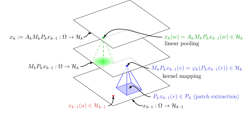
Figure 1: Construction of the $k$-th signal representation from the $k\text{--}1$-th one. Note that while the domain $\Omega$ is depicted as a box in ${\mathbb{R}}^{2}$ here, our construction is supported on $\Omega={\mathbb{R}}^{d}$.

Patch extraction operator.

Given the layer $x_{k\text{--}1}$, we consider a patch shape $S_{k}$, defined as a compact centered subset of ${{\mathbb{R}}^{d}}$, e.g., a box, and we define the Hilbert space ${\mathcal{P}}_{k}:=L^{2}(S_{k},{\mathcal{H}}_{k\text{--}1})$ equipped with the norm $\|z\|^{2}=\int_{S_{k}}\|z(u)\|^{2}d\nu_{k}(u)$, where $d\nu_{k}$ is the normalized uniform measure on $S_{k}$ for every $z$ in ${\mathcal{P}}_{k}$. Specifically, we define the (linear) patch extraction operator $P_{k}:L^{2}({{\mathbb{R}}^{d}},{\mathcal{H}}_{k\text{--}1})\to L^{2}({{\mathbb{R}}^{d}},{\mathcal{P}}_{k})$ such that for all $u$ in ${{\mathbb{R}}^{d}}$,

$$P_{k}x_{k\text{--}1}(u)=(v\mapsto x_{k\text{--}1}(u+v))_{v\in S_{k}}\in{\mathcal{P}}_{k}.$$

Note that by equipping ${\mathcal{P}}_{k}$ with a normalized measure, it is easy to show that the operator $P_{k}$ preserves the norm—that is, $\|P_{k}x_{k\text{--}1}\|=\|x_{k\text{--}1}\|$ and hence $P_{k}x_{k\text{--}1}$ is in $L^{2}({{\mathbb{R}}^{d}},{\mathcal{P}}_{k})$.

Kernel mapping operator.

Then, we map each patch of $x_{k\text{--}1}$ to a RKHS ${\mathcal{H}}_{k}$ thanks to the kernel mapping $\varphi_{k}:{\mathcal{P}}_{k}\to{\mathcal{H}}_{k}$ associated to a positive definite kernel $K_{k}$ that operates on patches. It allows us to define the pointwise operator $M_{k}$ such that for all $u$ in ${{\mathbb{R}}^{d}}$,

$$M_{k}P_{k}x_{k\text{--}1}(u):=\varphi_{k}(P_{k}x_{k\text{--}1}(u))\in{\mathcal{H}}_{k}.$$

In this paper, we consider homogeneous dot-product kernels $K_{k}$ operating on ${\mathcal{P}}_{k}$, defined in terms of a function $\kappa_{k}:[-1,1]\to{\mathbb{R}}$ that satisfies the following constraints:

$$\kappa_{k}(u)=\sum_{j=0}^{+\infty}b_{j}u^{j}\quad\text{s.t.}\quad\forall j,b_{j}\geq 0,\quad\kappa_{k}(1)=1,\quad\kappa_{k}^{\prime}(1)=1,$$ (A1)

assuming convergence of the series $\sum_{j}b_{j}$ and $\sum_{j}jb_{j}$. Then, we define the kernel $K_{k}$ by

$$K_{k}(z,z^{\prime})=\|z\|\|z^{\prime}\|\kappa_{k}\!\left(\frac{\langle z,z^{\prime}\rangle}{\|z\|\|z^{\prime}\|}\right),$$ (2)

if $z,z^{\prime}\in{\mathcal{P}}_{k}\setminus\{0\}$, and $K_{k}(z,z^{\prime})=0$ if $z=0$ or $z^{\prime}=0$. The kernel is positive definite since it admits a Maclaurin expansion with only non-negative coefficients (Schoenberg, 1942; Schölkopf and Smola, 2001). The condition $\kappa_{k}(1)=1$ ensures that the RKHS mapping preserves the norm—that is, $\|\varphi_{k}(z)\|=K_{k}(z,z)^{1/2}=\|z\|$, and thus $\|M_{k}P_{k}x_{k\text{--}1}(u)\|=\|P_{k}x_{k\text{--}1}(u)\|$ for all $u$ in ${{\mathbb{R}}^{d}}$; as a consequence, $M_{k}P_{k}x_{k\text{--}1}$ is always in $L^{2}({{\mathbb{R}}^{d}},{\mathcal{H}}_{k})$. The technical condition $\kappa_{k}^{\prime}(1)=1$, where $\kappa_{k}^{\prime}$ is the first derivative of $\kappa_{k}$, ensures that the kernel mapping $\varphi_{k}$ is non-expansive, according to Lemma 1 below.

Lemma 1 (Non-expansiveness of the kernel mappings)

Consider a positive-definite kernel of the form (2) satisfying (A1) with RKHS mapping $\varphi_{k}:{\mathcal{P}}_{k}\to{\mathcal{H}}_{k}$. Then, $\varphi_{k}$ is non-expansive—that is, for all $z,z^{\prime}$ in ${\mathcal{P}}_{k}$,

$$\|\varphi_{k}(z)-\varphi_{k}(z^{\prime})\|\leq\|z-z^{\prime}\|.$$

Moreover, we remark that the kernel $K_{k}$ is lower-bounded by the linear one

$$K_{k}(z,z^{\prime})\geq\langle z,z^{\prime}\rangle.$$ (3)

From the proof of the lemma, given in Appendix B, one may notice that the assumption $\kappa_{k}^{\prime}(1)=1$ is not critical and may be safely replaced by $\kappa_{k}^{\prime}(1)\leq 1$. Then, the non-expansiveness property would be preserved. Yet, we have chosen a stronger constraint since it yields a few simplifications in the stability analysis, where we use the relation (3) that requires $\kappa_{k}^{\prime}(1)=1$. More generally, the kernel mapping is Lipschitz continuous with constant $\rho_{k}=\max(1,\sqrt{\kappa_{k}^{\prime}(1)})$. Our stability results hold in a setting with $\rho_{k}>1$, but with constants $\prod_{k}\rho_{k}$ that may grow exponentially with the number of layers.

Examples of functions $\kappa_{k}$ that satisfy the properties (A1) are now given below:

exponential	$\kappa_{\text{exp}}(\langle z,z^{\prime}\rangle)=e^{\langle z,z^{\prime}\rangle-1}$
inverse polynomial	$\kappa_{\text{inv-poly}}(\langle z,z^{\prime}\rangle)=\frac{1}{2-\langle z,z^{\prime}\rangle}$
polynomial, degree $p$	$\kappa_{\text{poly}}(\langle z,z^{\prime}\rangle)=\frac{1}{(c+1)^{p}}(c+\langle z,z^{\prime}\rangle)^{p}~{}~{}~{}~{}\text{with}~{}~{}~{}c=p-1$
arc-cosine, degree 1	$\kappa_{\text{acos}}(\langle z,z^{\prime}\rangle)=\frac{1}{\pi}\left(\sin(\theta)+(\pi-\theta)\cos(\theta)\right)~{}\text{with}~{}\theta=\arccos(\langle z,z^{\prime}\rangle)$
Vovk’s, degree 3	$\kappa_{\text{vovk}}(\langle z,z^{\prime}\rangle)=\frac{1}{3}\left(\frac{1-\langle z,z^{\prime}\rangle^{3}}{1-\langle z,z^{\prime}\rangle}\right)=\frac{1}{3}\left(1+\langle z,z^{\prime}\rangle+\langle z,z^{\prime}\rangle^{2}\right)$

We note that the inverse polynomial kernel was used by Zhang et al. (2016, 2017b) to build convex models of fully connected networks and two-layer convolutional neural networks, while the arc-cosine kernel appears in early deep kernel machines (Cho and Saul, 2009). Note that the homogeneous exponential kernel reduces to the Gaussian kernel for unit-norm vectors. Indeed, for all $z,z^{\prime}$ such that $\|z\|=\|z^{\prime}\|=1$, we have

$$\kappa_{\text{exp}}(\langle z,z^{\prime}\rangle)=e^{\langle z,z^{\prime}\rangle-1}=e^{-\frac{1}{2}\|z-z^{\prime}\|^{2}},$$

and thus, we may refer to kernel (2) with the function $\kappa_{\text{exp}}$ as the homogeneous Gaussian kernel. The kernel $\kappa(\langle z,z^{\prime}\rangle)=e^{\alpha(\langle z,z^{\prime}\rangle-1)}=e^{-\frac{\alpha}{2}\|z-z^{\prime}\|^{2}}$ with $\alpha\neq 1$ may also be used here, but we choose $\alpha=1$ for simplicity since $\kappa^{\prime}(1)=\alpha$ (see discussion above).

Pooling operator.

The last step to build the layer $x_{k}$ consists of pooling neighboring values to achieve local shift-invariance. We apply a linear convolution operator $A_{k}$ with a Gaussian filter of scale $\sigma_{k}$, $h_{\sigma_{k}}(u):=\sigma_{k}^{-d}h(u/\sigma_{k})$, where $h(u)=(2\pi)^{-d/2}\exp(-|u|^{2}/2)$. Then, for all $u$ in ${{\mathbb{R}}^{d}}$,

$$x_{k}(u)=A_{k}M_{k}P_{k}x_{k\text{--}1}(u)=\int_{{\mathbb{R}}^{d}}h_{\sigma_{k}}(u-v)M_{k}P_{k}x_{k\text{--}1}(v)dv\in{\mathcal{H}}_{k},$$ (4)

where the integral is a Bochner integral (see, Diestel and Uhl, 1977; Muandet et al., 2017). By applying Schur’s test to the integral operator $A_{k}$ (see Appendix A), we obtain that the operator norm $\|A_{k}\|$ is less than $1$. Thus, $x_{k}$ is in $L^{2}({{\mathbb{R}}^{d}},{\mathcal{H}}_{k})$, with $\|x_{k}\|\leq\|M_{k}P_{k}x_{k\text{--}1}\|$. Note that a similar pooling operator is used in the scattering transform (Mallat, 2012).

Multilayer construction and prediction layer.

Finally, we obtain a multilayer representation by composing multiple times the previous operators. In order to increase invariance with each layer and to increase the size of the receptive fields (that is, the neighborhood of the original signal considered in a given patch), the size of the patch $S_{k}$ and pooling scale $\sigma_{k}$ typically grow exponentially with $k$, with $\sigma_{k}$ and the patch size $\sup_{c\in S_{k}}|c|$ of the same order. With $n$ layers, the maps $x_{n}$ may then be written

$$x_{n}:=A_{n}M_{n}P_{n}A_{n\text{--}1}M_{n\text{--}1}P_{n\text{--}1}\,\cdots\,A_{1}M_{1}P_{1}x_{0}~{}\in~{}L^{2}({{\mathbb{R}}^{d}},{\mathcal{H}}_{n}).$$ (5)

It remains to define a kernel from this representation, that will play the same role as the “fully connected” layer of classical convolutional neural networks. For that purpose, we simply consider the following linear kernel defined for all $x_{0},x_{0}^{\prime}$ in $L^{2}({{\mathbb{R}}^{d}},{\mathcal{H}}_{0})$ by using the corresponding feature maps $x_{n},x_{n}^{\prime}$ in $L^{2}({{\mathbb{R}}^{d}},{\mathcal{H}}_{n})$ given by our multilayer construction (5):

$${\mathcal{K}}_{n}(x_{0},x_{0}^{\prime})=\langle x_{n},x_{n}^{\prime}\rangle=\int_{u\in{{\mathbb{R}}^{d}}}\langle x_{n}(u),x_{n}^{\prime}(u)\rangle du.$$ (6)

Then, the RKHS ${\mathcal{H}}_{\mathcal{K}_{n}}$ of ${\mathcal{K}}_{n}$ contains all functions of the form $f(x_{0})=\langle w,x_{n}\rangle$ with $w$ in $L^{2}({{\mathbb{R}}^{d}},{\mathcal{H}}_{n})$ (see Appendix A).

We note that one may also consider nonlinear kernels, such as a Gaussian kernel:

$${\mathcal{K}}_{n}(x_{0},x_{0}^{\prime})=e^{-\frac{\alpha}{2}\|x_{n}-x_{n}^{\prime}\|^{2}}.$$ (7)

Such kernels are then associated to a RKHS denoted by ${\mathcal{H}}_{n+1}$, along with a kernel mapping $\varphi_{n+1}:L^{2}({{\mathbb{R}}^{d}},{\mathcal{H}}_{n})\to{\mathcal{H}}_{n+1}$ which we call prediction layer, so that the final representation is given by $\varphi_{n+1}(x_{n})$ in ${\mathcal{H}}_{n+1}$. We note that $\varphi_{n+1}$ is non-expansive for the Gaussian kernel when $\alpha\leq 1$ (see Section B.1), and is simply an isometric linear mapping for the linear kernel. Then, we have the relation ${\mathcal{K}}_{n}(x_{0},x_{0}^{\prime}):=\langle\varphi_{n+1}(x_{n}),\varphi_{n+1}(x_{n}^{\prime})\rangle,$ and in particular, the RKHS ${\mathcal{H}}_{\mathcal{K}_{n}}$ of ${\mathcal{K}}_{n}$ contains all functions of the form $f(x_{0})=\langle w,\varphi_{n+1}(x_{n})\rangle$ with $w$ in ${\mathcal{H}}_{n+1}$, see Appendix A.

2.1 Signal Preservation and Discretization

In this section, we show that the multilayer kernel representation preserves all information about the signal at each layer, and besides, each feature map $x_{k}$ can be sampled on a discrete set with no loss of information. This suggests a natural approach for discretization which will be discussed after the following lemma, whose proof is given in Appendix C.

Lemma 2 (Signal recovery from sampling)

Assume that ${\mathcal{H}}_{k}$ contains all linear functions $z\mapsto\langle g,z\rangle$ with $g$ in ${\mathcal{P}}_{k}$ (this is true for all kernels $K_{k}$ described in the previous section, according to Corollary 12 in Section 4.1 later); then, the signal $x_{k\text{--}1}$ can be recovered from a sampling of $x_{k}$ at discrete locations in a set $\Omega$ as soon as $\Omega+S_{k}={{\mathbb{R}}^{d}}$ (i.e., the union of patches centered at these points covers ${{\mathbb{R}}^{d}}$). It follows that $x_{k}$ can be reconstructed from such a sampling.

The previous construction defines a kernel representation for general signals in $L^{2}({{\mathbb{R}}^{d}},{\mathcal{H}}_{0})$, which is an abstract object defined for theoretical purposes. In practice, signals are discrete, and it is thus important to discuss the problem of discretization. For clarity, we limit the presentation to 1-dimensional signals ($d=1$), but the arguments can easily be extended to higher dimensions $d$ when using box-shaped patches. Notation from the previous section is preserved, but we add a bar on top of all discrete analogues of their continuous counterparts. e.g., $\bar{x}_{k}$ is a discrete feature map in $\ell^{2}({\mathbb{Z}},{\bar{\mathcal{H}}_{k}})$ for some RKHS $\bar{\mathcal{H}}_{k}$.

Input signals $x_{0}$ and $\bar{x}_{0}$.

Discrete signals acquired by a physical device may be seen as local integrators of signals defined on a continuous domain (e.g., sensors from digital cameras integrate the pointwise distribution of photons in a spatial and temporal window). Then, consider a signal $x_{0}$ in $L^{2}({{\mathbb{R}}^{d}},{\mathcal{H}}_{0})$ and $s_{0}$ a sampling interval. By defining $\bar{x}_{0}$ in $\ell_{2}({\mathbb{Z}},{\mathcal{H}}_{0})$ such that $\bar{x}_{0}[n]=x_{0}(ns_{0})$ for all $n$ in ${\mathbb{Z}}$, it is thus natural to assume that $x_{0}\!=\!A_{0}x$, where $A_{0}$ is a pooling operator (local integrator) applied to an original continuous signal $x$. The role of $A_{0}$ is to prevent aliasing and reduce high frequencies; typically, the scale $\sigma_{0}$ of $A_{0}$ should be of the same magnitude as $s_{0}$, which we choose to be $s_{0}=1$ without loss of generality. This natural assumption is kept later for the stability analysis.

Multilayer construction.

We now want to build discrete feature maps $\bar{x}_{k}$ in $\ell^{2}({\mathbb{Z}},\bar{\mathcal{H}}_{k})$ at each layer $k$ involving subsampling with a factor $s_{k}$ with respect to $\bar{x}_{k\text{--}1}$. We now define the discrete analogues of the operators $P_{k}$ (patch extraction), $M_{k}$ (kernel mapping), and $A_{k}$ (pooling) as follows: for $n\in{\mathbb{Z}}$,

$$\bar{P}_{k}\bar{x}_{k\text{--}1}[n] :=\frac{1}{\sqrt{e_{k}}}(\bar{x}_{k\text{--}1}[n],\bar{x}_{k\text{--}1}[n+1],\ldots,\bar{x}_{k\text{--}1}[n+e_{k}-1])\in\bar{{\mathcal{P}}}_{k}:=\bar{\mathcal{H}}_{k\text{--}1}^{e_{k}}$$

$$\bar{M}_{k}\bar{P}_{k}\bar{x}_{k\text{--}1}[n] :=\bar{\varphi}_{k}(\bar{P}_{k}\bar{x}_{k\text{--}1}[n])\in\bar{\mathcal{H}}_{k}$$

$$\bar{x}_{k}[n]\!=\!\bar{A}_{k}\bar{M}_{k}\bar{P}_{k}\bar{x}_{k\text{--}1}[n] :=\frac{1}{\sqrt{s_{k}}}\sum_{m\in{\mathbb{Z}}}\bar{h}_{k}[ns_{k}-m]\bar{M}_{k}\bar{P}_{k}\bar{x}_{k\text{--}1}[m]\!=\!(\bar{h}_{k}\ast\bar{M}_{k}\bar{P}_{k}\bar{x}_{k\text{--}1})[ns_{k}]\in\bar{\mathcal{H}}_{k},$$

where (i) $\bar{P}_{k}$ extracts a patch of size $e_{k}$ starting at position $n$ in $\bar{x}_{k\text{--}1}[n]$, which lives in the Hilbert space $\bar{{\mathcal{P}}}_{k}$ defined as the direct sum of $e_{k}$ times $\bar{{\mathcal{H}}}_{k\text{--}1}$; (ii) $\bar{M}_{k}$ is a kernel mapping identical to the continuous case, which preserves the norm, like $M_{k}$; (iii) $\bar{A}_{k}$ performs a convolution with a Gaussian filter and a subsampling operation with factor $s_{k}$. The next lemma shows that under mild assumptions, this construction preserves signal information.

Lemma 3 (Signal recovery with subsampling)

Assume that $\bar{\mathcal{H}}_{k}$ contains the linear functions $z\mapsto\langle w,z\rangle$ for all $w$ in $\bar{{\mathcal{P}}}_{k}$ and that $e_{k}\geq s_{k}$. Then, $\bar{x}_{k\text{--}1}$ can be recovered from $\bar{x}_{k}$.

The proof is given in Appendix C. The result relies on recovering patches using linear “measurement” functions and deconvolution of the pooling operation. While such a deconvolution operation can be unstable, it may be possible to obtain more stable recovery mechanisms by also considering non-linear measurements, a question which we leave open.

Links between the parameters of the discrete and continuous models.

Due to subsampling, the patch size in the continuous and discrete models are related by a multiplicative factor. Specifically, a patch of size $e_{k}$ with discretization corresponds to a patch $S_{k}$ of diameter $e_{k}s_{k-1}s_{k-2}\ldots s_{1}$ in the continuous case. The same holds true for the scale parameter $\sigma_{k}$ of the Gaussian pooling.

2.2 Practical Implementation via Convolutional Kernel Networks

Besides discretization, convolutional kernel networks add two modifications to implement in practice the image representation we have described. First, it uses feature maps with finite spatial support, which introduces border effects that we do not study (like Mallat, 2012), but which are negligible when dealing with large realistic images. Second, CKNs use finite-dimensional approximations of the kernel feature map. Typically, each RKHS’s mapping is approximated by performing a projection onto a subspace of finite dimension, which is a classical approach to make kernel methods work at large scale (Fine and Scheinberg, 2001; Smola and Schölkopf, 2000; Williams and Seeger, 2001). If we consider the kernel mapping $\varphi_{k}:{\mathcal{P}}_{k}\to{\mathcal{H}}_{k}$ at layer $k$, the orthogonal projection onto the finite-dimensional subspace $\mathcal{F}_{k}=\operatorname{span}(\varphi_{k}(z_{1}),\ldots,\varphi_{k}(z_{p_{k}}))\subseteq{\mathcal{H}}_{k}$, where the $z_{i}$’s are $p_{k}$ anchor points in ${\mathcal{P}}_{k}$, is given by the linear operator $\Pi_{k}:{\mathcal{H}}_{k}\to\mathcal{F}_{k}$ defined for $f$ in ${\mathcal{H}}_{k}$ by

$$\Pi_{k}f:=\sum_{1\leq i,j\leq p_{k}}(K_{ZZ}^{-1})_{ij}\langle\varphi_{k}(z_{i}),f\rangle\varphi_{k}(z_{j}),$$ (8)

where $K_{ZZ}^{-1}$ is the inverse (or pseudo-inverse) of the $p_{k}\times p_{k}$ kernel matrix $[K_{k}(z_{i},z_{j})]_{ij}$. As an orthogonal projection operator, $\Pi_{k}$ is non-expansive, i.e., $\|\Pi_{k}\|\leq 1$. We can then define the new approximate version $\tilde{M}_{k}$ of the kernel mapping operator $M_{k}$ by

$$\tilde{M}_{k}P_{k}x_{k\text{--}1}(u):=\Pi_{k}\varphi_{k}(P_{k}x_{k\text{--}1}(u))\in{\mathcal{F}}_{k}.$$ (9)

Note that all points in the feature map $\tilde{M}_{k}P_{k}x_{k\text{--}1}$ lie in the $p_{k}$-dimensional space $\mathcal{F}_{k}\subseteq{\mathcal{H}}_{k}$, which allows us to represent each point $\tilde{M}_{k}P_{k}x_{k\text{--}1}(u)$ by the finite dimensional vector

$$\psi_{k}(P_{k}x_{k\text{--}1}(u)):=K_{ZZ}^{-1/2}K_{Z}(P_{k}x_{k\text{--}1}(u))\in{\mathbb{R}}^{p_{k}},$$ (10)

with $K_{Z}(z):=(K_{k}(z_{1},z),\ldots,K_{k}(z_{p_{k}},z))^{\top}$; this finite-dimensional representation preserves the Hilbertian inner product and norm in ${\mathcal{F}}_{k}$ so that $\|\psi_{k}(P_{k}x_{k\text{--}1}(u))\|^{2}_{2}=\|\tilde{M}_{k}P_{k}x_{k\text{--}1}(u)\|^{2}_{{\mathcal{H}}_{k}}$.

Such a finite-dimensional mapping is compatible with the multilayer construction, which builds ${\mathcal{H}}_{k}$ by manipulating points from ${\mathcal{H}}_{k\text{--}1}$. Here, the approximation provides points in ${\mathcal{F}}_{k}\subseteq{\mathcal{H}}_{k}$, which remain in ${\mathcal{F}}_{k}$ after pooling since ${\mathcal{F}}_{k}$ is a linear subspace. Eventually, the sequence of RKHSs $\{{\mathcal{H}}_{k}\}_{k\geq 0}$ is not affected by the finite-dimensional approximation. Besides, the stability results we will present next are preserved thanks to the non-expansiveness of the projection. In contrast, other kernel approximations such as random Fourier features (Rahimi and Recht, 2007) do not provide points in the RKHS (see Bach, 2017), and their effect on the functional space derived from the multilayer construction is unclear.

It is then possible to derive theoretical results for the CKN model, which appears as a natural implementation of the kernel constructed previously; yet, we will also show in Section 4 that the results apply more broadly to CNNs that are contained in the functional space associated to the kernel. However, the stability of these CNNs depends on their RKHS norm, which is hard to control. In contrast, for CKNs, stability is typically controlled by the norm of the final prediction layer.

3 Stability to Deformations and Group Invariance

In this section, we study the translation invariance and the stability under the action of diffeomorphisms of the kernel representation described in Section 2 for continuous signals. In addition to translation invariance, it is desirable to have a representation that is stable to small local deformations. We describe such deformations using a $C^{1}$-diffeomorphism $\tau:{{\mathbb{R}}^{d}}\to{{\mathbb{R}}^{d}}$, and let $L_{\tau}$ denote the linear operator defined by $L_{\tau}x(u)=x(u-\tau(u))$. We use a similar characterization of stability to the one introduced by Mallat (2012): the representation $\Phi(\cdot)$ is stable under the action of diffeomorphisms if there exist two non-negative constants $C_{1}$ and $C_{2}$ such that

$$\|\Phi(L_{\tau}x)-\Phi(x)\|\leq(C_{1}\|\nabla\tau\|_{\infty}+C_{2}\|\tau\|_{\infty})\|x\|,$$ (11)

where $\nabla\tau$ is the Jacobian of $\tau$, $\|\nabla\tau\|_{\infty}\!:=\!\sup_{u\in{{\mathbb{R}}^{d}}}\|\nabla\tau(u)\|$, and $\|\tau\|_{\infty}\!:=\!\sup_{u\in{{\mathbb{R}}^{d}}}|\tau(u)|$. The quantity $\|\nabla\tau(u)\|$ measures the size of the deformation at a location $u$, and like Mallat (2012), we assume the regularity condition $\|\nabla\tau\|_{\infty}\leq 1/2$, which implies that the deformation is invertible (Allassonnière et al., 2007; Trouvé and Younes, 2005) and helps us avoid degenerate situations. In order to have a near-translation-invariant representation, we want $C_{2}$ to be small (a translation is a diffeomorphism with $\nabla\tau=0$), and indeed we will show that $C_{2}$ is proportional to $1/\sigma_{n}$, where $\sigma_{n}$ is the scale of the last pooling layer, which typically increases exponentially with the number of layers $n$. When $\nabla\tau$ is non-zero, the diffeomorphism deviates from a translation, producing local deformations controlled by $\nabla\tau$.

Additional assumptions.

In order to study the stability of the representation (5), we assume that the input signal $x_{0}$ may be written as $x_{0}=A_{0}x$, where $A_{0}$ is an initial pooling operator at scale $\sigma_{0}$, which allows us to control the high frequencies of the signal in the first layer. As discussed previously in Section 2.1, this assumption is natural and compatible with any physical acquisition device. Note that $\sigma_{0}$ can be taken arbitrarily small, so that this assumption does not limit the generality of our results. Then, we are interested in understanding the stability of the representation

$$\Phi_{n}(x):=A_{n}M_{n}P_{n}A_{n\text{--}1}M_{n\text{--}1}P_{n\text{--}1}\,\cdots\,A_{1}M_{1}P_{1}A_{0}x.$$

We do not consider a prediction layer $\varphi_{n+1}$ here for simplicity, but note that if we add one on top of $\Phi_{n}$, based on a linear of Gaussian kernel, then the stability of the full representation $\varphi_{n+1}\circ\Phi_{n}$ immediately follows from that of $\Phi_{n}$ thanks to the non-expansiveness of $\varphi_{n+1}$ (see Section 2). Then, we make an assumption that relates the scale of the pooling operator at layer $k-1$ with the diameter of the patch $S_{k}$: we assume indeed that there exists $\kappa>0$ such that for all $k\geq 1$,

$$\sup_{c\in S_{k}}|c|\leq\kappa\sigma_{k-1}.$$ (A2)

The scales $\sigma_{k}$ are typically exponentially increasing with the layers $k$, and characterize the “resolution” of each feature map. This assumption corresponds to considering patch sizes that are adapted to these intermediate resolutions. Moreover, the stability bounds we obtain hereafter increase with $\kappa$, which leads us to believe that small patch sizes lead to more stable representations, something which matches well the trend of using small, 3x3 convolution filters at each scale in modern deep architectures (e.g.,  Simonyan and Zisserman, 2014).

Finally, before presenting our stability results, we recall a few properties of the operators involved in the representation $\Phi_{n}$, which are heavily used in the analysis.

1. Patch extraction operator: $P_{k}$ is linear and preserves the norm; 2. Kernel mapping operator: $M_{k}$ preserves the norm and is non-expansive; 3. Pooling operator: $A_{k}$ is linear and non-expansive $\|A_{k}\|\leq 1$;

The rest of this section is organized into three parts. We present the main stability results in Section 3.1, explain their compatibility with kernel approximations in Section 3.3, and provide numerical experiment for demonstrating the stability of the kernel representation in Section 3.4. Finally, we introduce mechanisms to achieve invariance to any group of transformations in Section 3.5.

3.1 Stability Results and Translation Invariance

Here, we show that our kernel representation $\Phi_{n}$ satisfies the stability property (11), with a constant $C_{2}$ inversely proportional to $\sigma_{n}$, thereby achieving near-invariance to translations. The results are then extended to more general transformation groups in Section 3.5.

General bound for stability.

The following result gives an upper bound on the quantity of interest, $\|\Phi_{n}(L_{\tau}x)-\Phi_{n}(x)\|$, in terms of the norm of various linear operators which control how $\tau$ affects each layer. An important object of study is the commutator of linear operators $A$ and $B$, which is denoted by $[A,B]=AB-BA$.

Proposition 4 (Bound with operator norms)

For any $x$ in $L^{2}({{\mathbb{R}}^{d}},{\mathcal{H}}_{0})$, we have

$$\|\Phi_{n}(L_{\tau}x)-\Phi_{n}(x)\|\leq\left(\sum_{k=1}^{n}\|[P_{k}A_{k-1},L_{\tau}]\|+\|[A_{n},L_{\tau}]\|+\|L_{\tau}A_{n}-A_{n}\|\right)\|x\|.$$ (12)

For translations $L_{\tau}x(u)=L_{c}x(u)=x(u-c)$, it is easy to see that patch extraction and pooling operators commute with $L_{c}$ (this is also known as covariance or equivariance to translations), so that we are left with the term $\|L_{c}A_{n}-A_{n}\|$, which should control translation invariance. For general diffeomorphisms $\tau$, we no longer have exact covariance, but we show below that commutators are stable to $\tau$, in the sense that $\|[P_{k}A_{k-1},L_{\tau}]\|$ is controlled by $\|\nabla\tau\|_{\infty}$, while $\|L_{\tau}A_{n}-A_{n}\|$ is controlled by $\|\tau\|_{\infty}$ and decays with the pooling size $\sigma_{n}$.

Bound on $\|[P_{k}A_{k-1},L_{\tau}]\|$.

We note that $P_{k}z$ can be identified with $(L_{c}z)_{c\in S_{k}}$ isometrically for all $z$ in $L^{2}({{\mathbb{R}}^{d}},{\mathcal{H}}_{k\text{--}1})$, since $\|P_{k}z\|^{2}=\int_{S_{k}}\|L_{c}z\|^{2}d\nu_{k}(c)$ by Fubini’s theorem. Then,

$$\|P_{k}A_{k-1}L_{\tau}z-L_{\tau}P_{k}A_{k-1}z\|^{2} =\int_{S_{k}}\|L_{c}A_{k-1}L_{\tau}z-L_{\tau}L_{c}A_{k-1}z\|^{2}d\nu_{k}(c)$$

$$\leq\sup_{c\in S_{k}}\|L_{c}A_{k-1}L_{\tau}z-L_{\tau}L_{c}A_{k-1}z\|^{2},$$

so that $\|[P_{k}A_{k-1},L_{\tau}]\|\leq\sup_{c\in S_{k}}\|[L_{c}A_{k-1},L_{\tau}]\|$. The following result lets us bound the commutator $\|[L_{c}A_{k-1},L_{\tau}]\|$ when $|c|\leq\kappa\sigma_{k-1}$, which is satisfied under assumption (A2).

Lemma 5 (Stability of shifted pooling)

Consider $A_{\sigma}$ the pooling operator with kernel $h_{\sigma}(u)=\sigma^{-d}h(u/\sigma)$. If $\|\nabla\tau\|_{\infty}\leq 1/2$, there exists a constant $C_{1}$ such that for any $\sigma$ and $|c|\leq\kappa\sigma$, we have

$$\|[L_{c}A_{\sigma},L_{\tau}]\|\leq C_{1}\|\nabla\tau\|_{\infty},$$

where $C_{1}$ depends only on $h$ and $\kappa$.

A similar result can be found in Lemma E.1 of Mallat (2012) for commutators of the form $[A_{\sigma},L_{\tau}]$, but we extend it to handle integral operators $L_{c}A_{\sigma}$ with a shifted kernel. The proof (given in Appendix C.4) follows closely Mallat (2012) and relies on the fact that $[L_{c}A_{\sigma},L_{\tau}]$ is an integral operator in order to bound its norm via Schur’s test. Note that $\kappa$ can be made larger, at the cost of an increase of the constant $C_{1}$ of the order $\kappa^{d+1}$.

Bound on $\|L_{\tau}A_{n}-A_{n}\|$.

We bound the operator norm $\|L_{\tau}A_{n}-A_{n}\|$ in terms of $\|\tau\|_{\infty}$ using the following result due to Mallat (2012, Lemma 2.11), with $\sigma=\sigma_{n}$:

Lemma 6 (Translation invariance)

If $\|\nabla\tau\|_{\infty}\leq 1/2$, we have

$$\|L_{\tau}A_{\sigma}-A_{\sigma}\|\leq\frac{C_{2}}{\sigma}\|\tau\|_{\infty},$$

with $C_{2}=2^{d}\cdot\|\nabla h\|_{1}$.

Combining Proposition 4 with Lemmas 5 and 6, we now obtain the following result:

Theorem 7 (Stability bound)

Assume (A2). If $\|\nabla\tau\|_{\infty}\leq 1/2$, we have

$$\|\Phi_{n}(L_{\tau}x)-\Phi_{n}(x)\|\leq\left(C_{1}\left(1+n\right)\|\nabla\tau\|_{\infty}+\frac{C_{2}}{\sigma_{n}}\|\tau\|_{\infty}\right)\|x\|.$$ (13)

This result matches the desired notion of stability in Eq. (11), with a translation-invariance factor that decays with $\sigma_{n}$. We discuss implications of our bound, and compare it with related work on stability in Section 3.2. We also note that our bound yields a worst-case guarantee on stability, in the sense that it holds for any signal $x$. In particular, making additional assumptions on the signal (e.g., smoothness) may lead to improved stability. The predictions for a specific model may also be more stable than applying (1) to our stability bound, for instance if the filters are smooth enough.

Remark 8 (Stability for Lipschitz non-linear mappings)

While the previous results require non-expansive non-linear mappings $\varphi_{k}$, it is easy to extend the result to the following more general condition

$$\|\varphi_{k}(z)-\varphi_{k}(z^{\prime})\|\leq\rho_{k}\|z-z^{\prime}\|\quad\text{ and }\quad\|\varphi_{k}(z)\|\leq\rho_{k}\|z\|.$$

Indeed, the proof of Proposition 4 easily extends to this setting, giving an additional factor $\prod_{k}\rho_{k}$ in the bound (11). The stability bound (13) then becomes

$$\|\Phi_{n}(L_{\tau}x)-\Phi_{n}(x)\|\leq\left(\prod_{k=1}^{n}\rho_{k}\right)\left(C_{1}\left(1+n\right)\|\nabla\tau\|_{\infty}+\frac{C_{2}}{\sigma_{n}}\|\tau\|_{\infty}\right)\|x\|.$$ (14)

This will be useful for obtaining stability of CNNs with generic activations such as ReLU (see Section 4.3), and this also captures the case of kernels with $\kappa_{k}^{\prime}(1)>1$ in Lemma 1.

3.2 Discussion of the Stability Bound (Theorem 7)

In this section, we discuss the implications of our stability bound (13), and compare it to related work on the stability of the scattering transform (Mallat, 2012) as well as the work of (Wiatowski and Bölcskei, 2018) on more general convolutional models.

Role of depth.

Our bound displays a linear dependence on the number of layers $n$ in the stability constant $C_{1}(1+n)$. We note that a dependence on a notion of depth (the number of layers $n$ here) also appears in Mallat (2012), with a factor equal to the maximal length of “scattering paths”, and with the same condition $\|\nabla\tau\|_{\infty}\leq 1/2$. Nevertheless, the number of layers is tightly linked to the patch sizes, and we now show how a deeper architecture can be beneficial for stability. Given a desired level of translation-invariance $\sigma_{f}$ and a given initial resolution $\sigma_{0}$, the above bound together with the discretization results of Section 2.1 suggest that one can obtain a stable representation that preserves signal information by taking small patches at each layer and subsampling with a factor equal to the patch size (assuming a patch size greater than one) until the desired level of invariance is reached: in this case we have $\sigma_{f}/\sigma_{0}\approx\kappa^{n}$, where $\kappa$ is of the order of the patch size, so that $n=O(\log(\sigma_{f}/\sigma_{0})/\log(\kappa))$, and hence the stability constant $C_{1}(1+n)$ grows with $\kappa$ as $\kappa^{d+1}/\log(\kappa)$, explaining the benefit of small patches, and thus of deeper models.

Norm preservation.

While the scattering representation preserves the norm of the input signals when the length of scattering paths goes to infinity, in our setting the norm may decrease with depth due to pooling layers. However, we show in Appendix C.5 that a part of the signal norm is still preserved, particularly for signals with high energy in the low frequencies, as is the case for natural images (e.g., Torralba and Oliva, 2003). This justifies that the bounded quantity in (13) is relevant and non-trivial. Nevertheless, we recall that despite a possible loss in norm, our (infinite-dimensional) representation $\Phi(x)$ preserves signal information, as discussed in Section 2.1.

Dependence on signal bandwidth.

We note that our stability result crucially relies on the assumption $\sigma_{0}>0$, which effectively limits its applicability to signals with frequencies bounded by $\lambda_{0}\approx 1/\sigma_{0}$. While this assumption is realistic in practice for digital signals, our bound degrades as $\sigma_{0}$ approaches 0, since the number of layers $n$ grows as $\log(1/\sigma_{0})$, as explained above. This is in contrast to the stability bound of Mallat (2012), which holds uniformly over any such $\sigma_{0}$, thanks to the use of more powerful tools from harmonic analysis such as the Cotlar-Stein lemma, which allows to control stability simultaneously at all frequencies thanks to the structure of the wavelet transform, something which seems more challenging in our case due to the non-linearities separating different scales.

We note that it may be difficult to obtain meaningful stability results for an unbounded frequency support given a fixed architecture, without making assumptions about the filters of a specific model. In particular, if we consider a model with a high frequency Fourier or cosine filter at the first layer, supported on a large enough patch relative to the corresponding wavelength, this will cause instabilities, particularly if the input signal has isolated high frequencies (see, e.g., Bruna and Mallat, 2013). By the arguments of Section 4, such an unstable model $g$ is in the RKHS, and we then have that the final representation $\Phi(\cdot)$ is also unstable, since

$$\|\Phi(L_{\tau}x)-\Phi(x)\| =\sup_{f\in{\mathcal{H}}_{{\mathcal{K}}_{n}},\|f\|\leq 1}\langle f,\Phi(L_{\tau}x)-\Phi(x)\rangle$$

$$\geq\frac{1}{\|g\|}\langle g,\Phi(L_{\tau}x)-\Phi(x)\rangle=\frac{1}{\|g\|}(g(L_{\tau}x)-g(x)).$$

Comparison with Wiatowski and Bölcskei (2018).

The work of Wiatowski and Bölcskei (2018) also studies deformation stability for generic convolutional network models, however their “deformation sensitivity” result only shows that the representation is as sensitive to deformations as the original signal, something which is also applicable here thanks to the non-expansiveness of our representation. Moreover, their bound does not show the dependence on deformation size (the Jacobian norm), and displays a translation invariance part that degrades linearly with $1/\sigma_{0}$. In contrast, the translation invariance part of our bound is independent of $\sigma_{0}$, and the overall bound only depends logarithmically on $1/\sigma_{0}$, by exploiting architectural choices such as pooling layers and patch sizes.

3.3 Stability with Kernel Approximations

As in the analysis of the scattering transform of Mallat (2012), we have characterized the stability and shift-invariance of the data representation for continuous signals, in order to give some intuition about the properties of the corresponding discrete representation, which we have described in Section 2.1.

Another approximation performed in the CKN model of Mairal (2016) consists of adding projection steps on finite-dimensional subspaces of the RKHS’s layers, as discusssed in Section 2.2. Interestingly, the stability properties we have obtained previously are compatible with these steps. We may indeed replace the operator $M_{k}$ with the operator $\tilde{M}_{k}z(u)=\Pi_{k}\varphi_{k}(z(u))$ for any map $z$ in $L^{2}({{\mathbb{R}}^{d}},{\mathcal{P}}_{k})$, instead of $M_{k}z(u)=\varphi_{k}(z(u))$; $\Pi_{k}:{\mathcal{H}}_{k}\to{\mathcal{F}}_{k}$ is here an orthogonal projection operator onto a linear subspace, given in (8). Then, $\tilde{M}_{k}$ does not necessarily preserve the norm anymore, but $\|\tilde{M}_{k}z\|\leq\|z\|$, with a loss of information equal to $\|M_{k}z-\tilde{M}_{k}z\|$ corresponding to the quality of approximation of the kernel $K_{k}$ on the points $z(u)$. On the other hand, the non-expansiveness of $M_{k}$ is satisfied thanks to the non-expansiveness of the projection. In summary, it is possible to show that the conclusions of Theorem 7 remain valid when adding the CKN projection steps at each layer, but some signal information is lost in the process.

3.4 Empirical Study of Stability

In this section, we provide numerical experiments to demonstrate the stability properties of the kernel representations defined in Section 2 on discrete images.

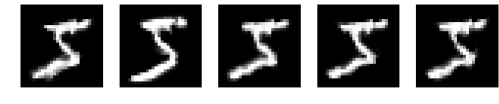
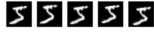
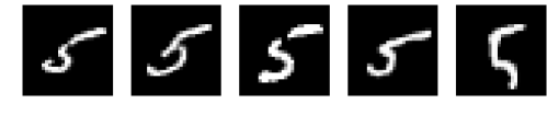
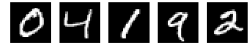
Figure 2: MNIST digits with transformations considered in our numerical study of stability. Each row gives examples of images from a set of digits that are compared to a reference image of a “5”. From top to bottom: deformations with $\alpha=3$; translations and deformations with $\alpha=1$; digits from the training set with the same label “5” as the reference digit; digits from the training set with any label.

We consider images of handwritten digits from the Infinite MNIST dataset of Loosli et al. (2007), which consists of 28x28 grayscale MNIST digits augmented with small translations and deformations. Translations are chosen at random from one of eight possible directions, while deformations are generated by considering small smooth deformations $\tau$, and approximating $L_{\tau}x$ using a tangent vector field $\nabla x$ containing partial derivatives of the signal $x$ along the horizontal and vertical image directions. We introduce a deformation parameter $\alpha$ to control such deformations, which are then given by

$$L_{\alpha\tau}x(u)=x(u-\alpha\tau(u))\approx x(u)-\alpha\tau(u)\cdot\nabla x(u).$$

Figure 2 shows examples of different deformations, with various values of $\alpha$, with or without translations, generated from a reference image of the digit “5”. In addition, one may consider that a given reference image of a handwritten digit can be deformed into different images of the same digit, and perhaps even into a different digit (e.g., a “1” may be deformed into a “7”). Intuitively, the latter transformation corresponds to a “larger” deformation than the former, so that a prediction function that is stable to deformations should be preferable for a classification task. The aim of our experiments is to quantify this stability, and to study how it is affected by architectural choices such as patch sizes and pooling scales.

We consider a full kernel representation, discretized as described in Section 2.1. We limit ourselves to 2 layers in order to make the computation of the full kernel tractable. Patch extraction is performed with zero padding in order to preserve the size of the previous feature map. We use a homogeneous dot-product kernel as in Eq. (2) with $\kappa(z)=e^{\rho(z-1)}$, $\rho=1/(0.65)^{2}$. Note that this choice yields $\kappa^{\prime}(z)=\rho>1$, giving an $\rho$-Lipschitz kernel mapping instead of a non-expansive one as in Lemma 1 which considers $\rho=1$. However, values of $\rho$ larger than one typically lead to better empirical performance for classification (Mairal, 2016), and the stability results of Section 3 are still valid with an additional factor $\rho^{n}$ (with $n=2$ here) in Eq. (13). For a subsampling factor $s$, we apply a Gaussian filter with scale $\sigma=s/\sqrt{2}$ before downsampling. Our C++ implementation for computing the full kernel given two images is available at https://github.com/albietz/ckn_kernel.

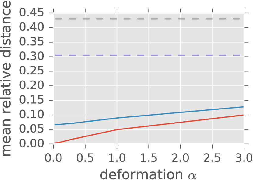
(a)

(b)

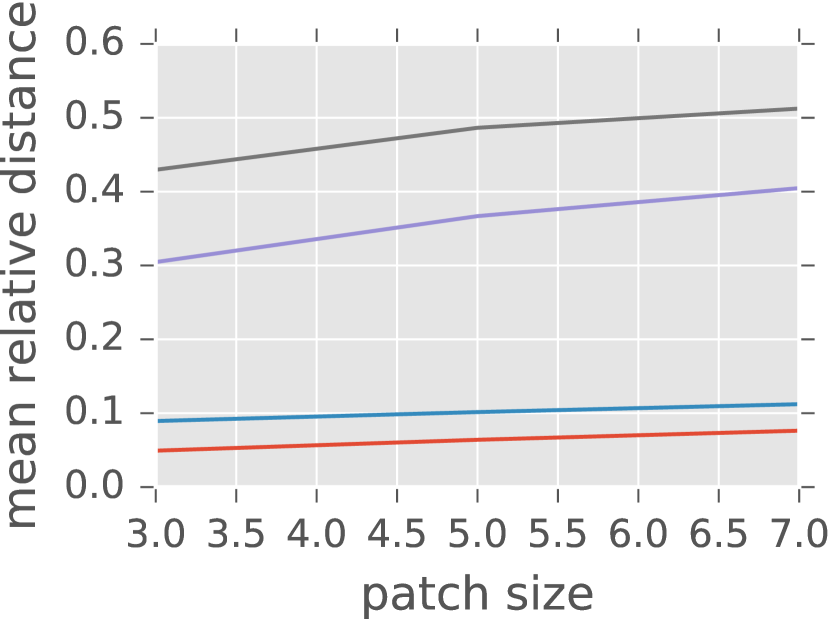
(c)

Figure 3: Average relative representation distance for various 2-layer models. Lines in the legend corresponds to rows of images in Figure 2. In (b-c), deformations are obtained with $\alpha=1$. We show the impact on relative distance of: (a) the value of $\alpha$ in deformations, in $\{0.01,0.03,0.1,0.3,1,3\}$; (b) the subsampling factor of the final pooling layer, in $\{1,3,5\}$; (c) the patch size, in $\{3,5,7\}$.

In Figure 3, we show average relative distance in representation space between a reference image and images from various sets of 20 images (either generated transformations, or images appearing in the training set). For a given architecture $A$ and set $S$ of images, the average relative distance to an image $x$ is given by

$$\frac{1}{|S|}\sum_{x^{\prime}\in S}\frac{\|\Phi_{A}(x^{\prime})-\Phi_{A}(x)\|}{\|\Phi_{A}(x)\|}=\frac{1}{|S|}\sum_{x^{\prime}\in S}\frac{\sqrt{K_{A}(x,x)+K_{A}(x^{\prime},x^{\prime})-2K_{A}(x,x^{\prime})}}{\sqrt{K_{A}(x,x)}},$$

where $\Phi_{A}$ denotes the kernel representation for architecture $A$ and $K_{A}(x,x^{\prime})$ the corresponding kernel. We normalize by $\|\Phi_{A}(x)\|$ in order to reduce sensitivity to the choice of architecture. We start with a $(3,2)$-layer followed by a $(3,5)$-layer, where $(p,s)$ indicates a layer with patch size $p$ and subsampling $s$. In Figure 3(b), we vary the subsampling factor of the second layer, and in Figure 3(c) we vary the patch size of both layers.

Each row of Figure 2 shows digits and deformed versions. Intuitively, it should be easier to deform an image of a handwritten 5 into a different image of a 5, than into a different digit. Indeed, Figure 3 shows that the average relative distance for images with different labels is always larger than for images with the same label, which in turn is larger than for small deformations and translations of the reference image.

Adding translations on top of deformations increases distance in all cases, and Figure 3(b) shows that this gap is smaller when using larger subsampling factors in the last layer. This agrees with the stability bound (13), which shows that a larger pooling scale at the last layer increases translation invariance. Figure 3(a) highlights the dependence of the distance on the deformation size $\alpha$, which is near-linear as in Eq. (13) (note that $\alpha$ controls the Jacobian of the deformation). Finally, Figure 3(c) shows that larger patch sizes can make the representations less stable, as discussed in Section 3.

3.5 Global Invariance to Group Actions

In Section 3.1, we have seen how the kernel representation of Section 2 creates invariance to translations by commuting with the action of translations at intermediate layers, and how the last pooling layer on the translation group governs the final level of invariance. It is often useful to encode invariances to different groups of transformations, such as rotations or reflections (see, e.g.,  Cohen and Welling, 2016; Mallat, 2012; Raj et al., 2017; Sifre and Mallat, 2013). Here, we show how this can be achieved by defining adapted patch extraction and pooling operators that commute with the action of a transformation group $G$ (this is known as group covariance or equivariance). We assume that $G$ is locally compact such that we can define a left-invariant Haar measure $\mu$—that is, a measure on $G$ that satisfies $\mu(gS)=\mu(S)$ for any Borel set $S\subseteq G$ and $g$ in $G$. We assume the initial signal $x(u)$ is defined on $G$, and we define subsequent feature maps on the same domain. The action of an element $g$ in $G$ is denoted by $L_{g}$, where $L_{g}x(u)=x(g^{-1}u)$. In order to keep the presentation simple, we ignore some issues related to the general construction in $L^{2}(G)$ of our signals and operators, which can be made more precise using tools from abstract harmonic analysis (e.g., Folland, 2016).

Extending a signal on $G$.

We note that the original signal is defined on a domain ${{\mathbb{R}}^{d}}$ which may be different from the transformation group $G$ that acts on ${{\mathbb{R}}^{d}}$ (e.g., for 2D images the domain is ${\mathbb{R}}^{2}$ but $G$ may also include a rotation angle). The action of $g$ in $G$ on the original signal defined on ${{\mathbb{R}}^{d}}$, denoted $\tilde{x}(\omega)$ yields a transformed signal $L_{g}\tilde{x}(\omega)=\tilde{x}(g^{-1}\cdot\omega)$, where $\cdot$ denotes group action. This requires an appropriate extension of the signal to $G$ that preserves the meaning of signal transformations. We make the following assumption: every element $\omega$ in ${{\mathbb{R}}^{d}}$ can be reached with a transformation $u_{\omega}$ in $G$ from a neutral element $\epsilon$ in ${{\mathbb{R}}^{d}}$ (e.g., $\epsilon=0$), as $\omega=u_{\omega}\cdot\epsilon$. Note that for 2D images ($d=2$), this typically requires a group $G$ that is “larger” than translations, such as the roto-translation group, while it is not satisfied, for instance, for rotations only. A similar assumption is made by Kondor and Trivedi (2018). Then, one can extend the original signal $\tilde{x}$ by defining $x(u):=\tilde{x}(u\cdot\epsilon)$. Indeed, we then have

$$L_{g}x(u_{\omega})=x(g^{-1}u_{\omega})=\tilde{x}((g^{-1}u_{\omega})\cdot\epsilon)=\tilde{x}(g^{-1}\cdot\omega),$$

so that the signal $(x(u_{\omega}))_{\omega\in{{\mathbb{R}}^{d}}}$ preserves the structure of $\tilde{x}$. We detail this below for the example of roto-translations on 2D images. Then, we are interested in defining a layer—that is, a succession of patch extraction, kernel mapping, and pooling operators—that commutes with $L_{g}$, in order to achieve equivariance to $G$.

Patch extraction.

We define patch extraction as follows

$$Px(u)=(x(uv))_{v\in S}~{}~{}~{}~{}\text{for all}~{}~{}u\in G,$$

where $S\subset G$ is a patch shape centered at the identity element. $P$ commutes with $L_{g}$ since

$$PL_{g}x(u)=(L_{g}x(uv))_{v\in S}=(x(g^{-1}uv))_{v\in S}=Px(g^{-1}u)=L_{g}Px(u).$$

Kernel mapping.

The pointwise operator $M$ is defined exactly as in Section 2, and thus commutes with $L_{g}$.

Pooling.

The pooling operator on the group $G$ is defined by

$$Ax(u)=\int_{G}x(uv)h(v)d\mu(v)=\int_{G}x(v)h(u^{-1}v)d\mu(v),$$

where $h$ is a pooling filter typically localized around the identity element. The construction is similar to Raj et al. (2017) and it is easy to see from the first expression of $Ax(u)$ that $AL_{g}x(u)=L_{g}Ax(u)$, making the pooling operator $G$-equivariant. One may also pool on a subset of the group by only integrating over the subset in the first expression, an operation which is also $G$-equivariant.

In our analysis of stability in Section 3.1, we saw that inner pooling layers are useful to guarantee stability to local deformations, while global invariance is achieved mainly through the last pooling layer. In some cases, one only needs stability to a subgroup of $G$, while achieving invariance to the whole group, e.g., in the roto-translation group (Oyallon and Mallat, 2015; Sifre and Mallat, 2013), one might want invariance to a global rotation but stability to local translations. Then, one can perform patch extraction and pooling just on the subgroup to stabilize (e.g., translations) in intermediate layers, while pooling on the entire group at the last layer to achieve the global group invariance.

Example with the roto-translation group.

We consider a simple example on 2D images where one wants global invariance to rotations in addition to near-invariance and stability to translations as in Section 3.1. For this, we consider the roto-translation group (see, e.g., Sifre and Mallat, 2013), defined as the semi-direct product of translations ${\mathbb{R}}^{2}$ and rotations $SO(2)$, denoted by $G={\mathbb{R}}^{2}\rtimes SO(2)$, with the following group operation

$$gg^{\prime}=(v+R_{\theta}v^{\prime},\theta+\theta^{\prime}),$$

for $g=(v,\theta)$, $g^{\prime}=(v^{\prime},\theta^{\prime})$ in $G$, where $R_{\theta}$ is a rotation matrix in $SO(2)$. The element $g=(v,\theta)$ in $G$ acts on a location $u\in{\mathbb{R}}^{2}$ by combining a rotation and a translation:

$$g\cdot u =v+R_{\theta}u$$

$$g^{-1}\cdot u =(-R_{-\theta}v,-\theta)\cdot u=R_{-\theta}(u-v).$$

For a given image $\tilde{x}$ in $L^{2}({\mathbb{R}}^{2})$, our equivariant construction outlined above requires an extension of the signal to the group $G$. We consider the Haar measure given by $d\mu((v,\theta)):=dvd\mu_{c}(\theta)$, where $dv$ is the Lebesgue measure on ${\mathbb{R}}^{2}$ and $d\mu_{c}$ the normalized Haar measure on the unit circle. Note that $\mu$ is left-invariant, since the determinant of rotation matrices that appears in the change of variables is 1. We can then define $x$ by $x((u,\eta)):=\tilde{x}(u)$ for any angle $\eta$, which is in $L^{2}(G)$ and preserves the definition of group action on the original signal $\tilde{x}$ since

$$L_{g}x((u,\eta))=x(g^{-1}(u,\eta))=x((g^{-1}\cdot u,\eta-\theta))=\tilde{x}(g^{-1}\cdot u)=L_{g}\tilde{x}(u).$$

That is, we can study the action of $G$ on 2D images in $L^{2}({\mathbb{R}}^{2})$ by studying the action on the extended signals in $L^{2}(G)$ defined above.

We can now define patch extraction and pooling operators $P,A:L^{2}(G)\to L^{2}(G)$ only on the translation subgroup, by considering a patch shape $S=\{(v,0)\}_{v\in\tilde{S}}\subset G$ with $\tilde{S}\subset{\mathbb{R}}^{2}$ for $P$, and defining pooling by $Ax(g)=\int_{{\mathbb{R}}^{d}}x(g(v,0))h(v)dv,$ where $h$ is a Gaussian pooling filter with scale $\sigma$ defined on ${\mathbb{R}}^{2}$.

The following result, proved in Appendix C, shows analogous results to the stability lemmas of Section 3.1 for the operators $P$ and $A$. For a diffeomorphism $\tau$, we denote by $L_{\tau}$ the action operator given by $L_{\tau}x((u,\eta))=x((\tau(u),0)^{-1}(u,\eta))=x((u-\tau(u),\eta))$.

Lemma 9 (Stability with roto-translation patches)

If $\|\nabla\tau\|_{\infty}\leq 1/2$, and the following condition holds $\sup_{c\in\tilde{S}}|c|\leq\kappa\sigma$, we have

$$\|[PA,L_{\tau}]\|\leq C_{1}\|\nabla\tau\|_{\infty},$$

with the same constant $C_{1}$ as in Lemma 5, which depends on $h$ and $\kappa$. Similarly, we have

$$\|L_{\tau}A-A\|\leq\frac{C_{2}}{\sigma}\|\tau\|_{\infty},$$

with $C_{2}$ as defined in Lemma 6.

By constructing a multi-layer representation $\Phi_{n}(x)$ in $L^{2}(G)$ using similar operators at each layer, we can obtain a similar stability result to Theorem 7. By adding a global pooling operator $A_{c}:L^{2}(G)\to L^{2}({\mathbb{R}}^{2})$ after the last layer, defined, for $x\in L^{2}(G)$, as

$$A_{c}x(u)=\int x((u,\eta))d\mu_{c}(\eta),$$

we additionally obtain global invariance to rotations, as shown in the following theorem.

Theorem 10 (Stability and global rotation invariance)

Assume (A2) for patches $\tilde{S}$ at each layer. Define the operator $L_{(\tau,\theta)}x((u,\eta))=x((\tau(u),\theta)^{-1}(u,\eta))$, and define the diffeomorphism $\tau_{\theta}:u\mapsto R_{-\theta}\tau(u)$. If $\|\nabla\tau\|_{\infty}\leq 1/2$, we have

$$\|A_{c}\Phi_{n}(L_{(\tau,\theta)}x)-A_{c}\Phi_{n}(x)\| \leq\|\Phi_{n}(L_{R_{\tau_{\theta}}}x)-\Phi_{n}(x)\|$$

$$\leq\left(C_{1}\left(1+n\right)\|\nabla\tau\|_{\infty}+\frac{C_{2}}{\sigma_{n}}\|\tau\|_{\infty}\right)\|x\|.$$

We note that a similar result may be obtained when $G={{\mathbb{R}}^{d}}\rtimes H$, where $H$ is any compact group, with a possible additional dependence on how elements of $H$ affect the size of patches.

4 Link with Existing Convolutional Architectures

In this section, we study the functional spaces (RKHS) that arise from our multilayer kernel representation, and examine the connections with more standard convolutional architectures. The motivation of this study is that if a CNN model $f$ is in the RKHS, then it can be written in a “linearized” form $f(x)=\langle f,\Phi(x)\rangle$, so that our study of stability of the kernel representation $\Phi$ extends to predictions using $|f(x)-f(x^{\prime})|\leq\|f\|\|\Phi(x)-\Phi(x^{\prime})\|$.

We begin by considering in Section 4.1 the intermediate kernels $K_{k}$, showing that their RKHSs contain simple neural-network-like functions defined on patches with smooth activations, while in Section 4.2 we show that a certain class of generic CNNs are contained in the RKHS ${\mathcal{H}}_{{\mathcal{K}}_{n}}$ of the full multilayer kernel ${\mathcal{K}}_{n}$ and characterize their norm. This is achieved by considering particular functions in each intermediate RKHS defined in terms of the convolutional filters of the CNN. A consequence of these results is that our stability and invariance properties from Section 3 are valid for this broad class of CNNs.

4.1 Activation Functions and Kernels $K_{k}$

Before introducing formal links between our kernel representation and classical convolutional architectures, we study in more details the kernels $K_{k}$ described in Section 2 and their RKHSs ${\mathcal{H}}_{k}$. In particular, we are interested in characterizing which types of functions live in ${\mathcal{H}}_{k}$. The next lemma extends some results of Zhang et al. (2016, 2017b), originally developed for the inverse polynomial and Gaussian kernels; it shows that the RKHS may contain simple “neural network” functions with activations $\sigma$ that are smooth enough.

Lemma 11 (Activation functions and RKHSs ${\mathcal{H}}_{k}$)

Let $\sigma:[-1,1]\to{\mathbb{R}}$ be a function that admits a polynomial expansion $\sigma(u):=\sum_{j=0}^{\infty}a_{j}u^{j}$. Consider a kernel $K_{k}$ from Section 2, given in (2), with $\kappa_{k}(u)=\sum_{j=0}^{\infty}b_{j}u^{j}$, and $b_{j}\geq 0$ for all $j$. Assume further that $a_{j}=0$ whenever $b_{j}=0$, and define the function $C_{\sigma}^{2}(\lambda^{2}):=\sum_{j=0}^{\infty}(a_{j}^{2}/b_{j})\lambda^{2j}$. Let $g$ in ${\mathcal{P}}_{k}$ be such that $C_{\sigma}^{2}(\|g\|^{2})<\infty$. Then, the RKHS ${\mathcal{H}}_{k}$ contains the function

$$f:z\mapsto\|z\|\sigma(\langle g,z\rangle/\|z\|),$$ (15)

and its norm satisfies $\|f\|\leq C_{\sigma}(\|g\|^{2})$.

Noting that for all examples of $\kappa_{k}$ given in Section 2, we have $b_{1}>0$, this result implies the next corollary, which was also found to be useful in our analysis.

Corollary 12 (Linear functions and RKHSs)

The RKHSs ${\mathcal{H}}_{k}$ for the examples of $\kappa_{k}$ given in Section 2 contain all linear functions of the form $z\mapsto\langle g,z\rangle$ with $g$ in ${\mathcal{P}}_{k}$.

The previous lemma shows that for many choices of smooth functions $\sigma$, the RKHS ${\mathcal{H}}_{k}$ contains the functions of the form (15). While the non-homogeneous functions $z\mapsto\sigma(\langle g,z\rangle)$ are standard in neural networks, the homogeneous variant is not. Yet, we note that (i) the most successful activation function, namely rectified linear units, is homogeneous—that is, $\text{relu}(\langle g,z\rangle)=\|z\|\text{relu}(\langle g,z\rangle/\|z\|)$; (ii) while relu is nonsmooth and thus not in our RKHSs, there exists a smoothed variant that satisfies the conditions of Lemma 11 for useful kernels. As noticed by Zhang et al. (2016, 2017b), this is for instance the case for the inverse polynomial kernel. In Figure 4, we plot and compare these different variants of ReLU.

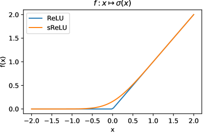
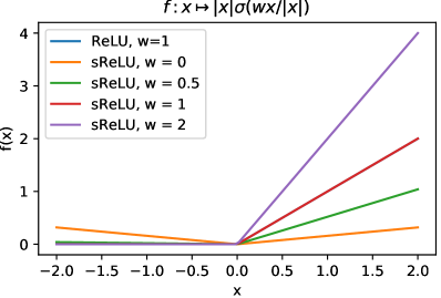
Figure 4: Comparison of one-dimensional functions obtained with relu and smoothed relu (sReLU) activations. (Left) non-homogeneous setting of Zhang et al. (2016, 2017b). (Right) our homogeneous setting, for different values of the parameter $w$. Note that for $w\geq 0.5$, sReLU and ReLU are indistinguishable.

4.2 Convolutional Neural Networks and their Complexity

We now study the connection between the kernel representation defined in Section 2 and CNNs. Specifically, we show that the RKHS of the final kernel ${\mathcal{K}}_{n}$ obtained from our kernel construction contains a set of CNNs on continuous domains with certain types of smooth homogeneous activations. An important consequence is that the stability results of previous sections apply to this class of CNNs, although the stability depends on the RKHS norm, as discussed later in Section 5. This norm also serves as a measure of model complexity, thus controlling both generalization and stability.

CNN maps construction.

We now define a CNN function $f_{\sigma}$ that takes as input an image $z_{0}$ in $L^{2}({{\mathbb{R}}^{d}},{\mathbb{R}}^{p_{0}})$ with $p_{0}$ channels, and build a sequence of feature maps, represented at layer $k$ as a function $z_{k}$ in $L^{2}({{\mathbb{R}}^{d}},{\mathbb{R}}^{p_{k}})$ with $p_{k}$ channels; the map $z_{k}$ is obtained from $z_{k\text{--}1}$ by performing linear convolutions with a set of filters $(w_{k}^{i})_{i=1,\ldots,p_{k}}$, followed by a pointwise activation function $\sigma$ to obtain an intermediate feature map $\tilde{z}_{k}$, then by applying a linear pooling filter. Note that each $w_{k}^{i}$ is in $L^{2}(S_{k},{\mathbb{R}}^{p_{k\text{--}1}})$, with channels denoted by $w_{k}^{ij}$ in $L^{2}(S_{k},{\mathbb{R}})$. Formally, the intermediate map $\tilde{z}_{k}$ in $L^{2}({{\mathbb{R}}^{d}},{\mathbb{R}}^{p_{k}})$ is obtained by

$$\tilde{z}_{k}^{i}(u)=n_{k}(u)\sigma\!\left(\langle w_{k}^{i},P_{k}z_{k\text{--}1}(u)\rangle/n_{k}(u)\right),$$ (16)

where $\tilde{z}_{k}(u)=(\tilde{z}_{k}^{1}(u),\ldots,\tilde{z}_{k}^{p_{k}}(u))$ is in ${\mathbb{R}}^{p_{k}}$, and $P_{k}$ is a patch extraction operator for finite-dimensional maps. The activation involves a pointwise non-linearity $\sigma$ along with a quantity $n_{k}(u):=\|P_{k}x_{k-1}(u)\|$ in (16), which is due to the homogenization, and which is independent of the filters $w_{k}^{i}$. Finally, the map $z_{k}$ is obtained by using a pooling operator as in Section 2, with $z_{k}=A_{k}\tilde{z}_{k}$, and $z_{0}=x_{0}$.

Prediction layer.

For simplicity, we consider the case of a linear fully connected prediction layer. In this case, the final CNN prediction function $f_{\sigma}$ is given by

$$f_{\sigma}(x_{0})=\langle w_{n+1},z_{n}\rangle,$$

with parameters $w_{n+1}$ in $L^{2}({{\mathbb{R}}^{d}},{\mathbb{R}}^{p_{n}})$. We now show that such a CNN function is contained in the RKHS of the kernel ${\mathcal{K}}_{n}$ defined in (6).

Construction in the RKHS.

The function $f_{\sigma}$ can be constructed recursively from intermediate functions that lie in the RKHSs ${\mathcal{H}}_{k}$, of the form (15), for appropriate activations $\sigma$. Specifically, we define initial quantities $f_{1}^{i}$ in $\mathcal{H}_{1}$ and $g^{i}_{1}$ in ${\mathcal{P}}_{1}$ for $i=1,\ldots,p_{1}$ such that

$$g_{1}^{i} =w_{1}^{i}\in L^{2}(S_{1},{\mathbb{R}}^{p_{0}})=L^{2}(S_{1},{\mathcal{H}}_{0})={\mathcal{P}}_{1},$$

$$f_{1}^{i}(z) =\|z\|\sigma(\langle g^{0}_{i},z\rangle/\|z\|)\quad\text{ for }z\in{\mathcal{P}}_{1},$$

and we define, from layer $k\text{--}1$, the quantities $f_{k}^{i}$ in $\mathcal{H}_{k}$ and $g_{k}^{i}$ in ${\mathcal{P}}_{k}$ for $i=1,\ldots,p_{k}$:

$$g_{k}^{i}(v) =\sum_{j=1}^{p_{k\text{--}1}}w_{k}^{ij}(v)f_{k\text{--}1}^{j}~{}~{}~{}\text{where}~{}~{}~{}w_{k}^{i}(v)=(w_{k}^{ij}(v))_{j=1,\ldots,p_{k\text{--}1}},$$

$$f_{k}^{i}(z) =\|z\|\sigma(\langle g_{k}^{i},z\rangle/\|z\|)\quad\text{ for }z\in{\mathcal{P}}_{k}.$$

For the linear prediction layer, we define $g_{\sigma}$ in $L^{2}({{\mathbb{R}}^{d}},{\mathcal{H}}_{n})$ by:

$$g_{\sigma}(u) =\sum_{j=1}^{p_{n}}w_{n+1}^{j}(u)f_{n}^{j}\quad\text{ for all }u\in{{\mathbb{R}}^{d}},$$

so that the function $f:x_{0}\mapsto\langle g_{\sigma},x_{n}\rangle$ is in the RKHS of ${\mathcal{K}}_{n}$, where $x_{n}$ is the final representation given in Eq. (5). In Appendix D.2, we show that $f=f_{\sigma}$, which implies that the CNN function $f_{\sigma}$ is in the RKHS. We note that a similar construction for fully connected multilayer networks with constraints on weights and inputs was given by Zhang et al. (2016).

Norm of the CNN $f_{\sigma}$.

We now study the RKHS norm of the CNN constructed above. This quantity is important as it controls the stability and invariance of the predictions of a learned model through (1). Additionally, the RKHS norm provides a way to control model complexity, and can lead to generalization bounds, e.g., through Rademacher complexity and margin bounds (Boucheron et al., 2005; Shalev-Shwartz and Ben-David, 2014). In particular, such results rely on the following upper bound on the empirical Rademacher complexity of a function class with bounded RKHS norm $\mathcal{F}_{\lambda}=\{f\in{\mathcal{H}}_{\mathcal{K}_{n}}:\|f\|\leq\lambda\}$, for a dataset $\{x^{(1)},\ldots,x^{(N)}\}$:

$$R_{N}(\mathcal{F}_{\lambda})\leq\frac{\lambda\sqrt{\frac{1}{N}\sum_{i=1}^{N}{\mathcal{K}}_{n}(x^{(i)},x^{(i)})}}{\sqrt{N}}.$$ (17)

The bound remains valid when only considering CNN functions in $\mathcal{F}_{\lambda}$ of the form $f_{\sigma}$, since such a function class is contained in $\mathcal{F}_{\lambda}$. If we consider a binary classification task with training labels $y^{(i)}$ in $\{-1,1\}$, on can then obtain a margin-based bound for any function $f_{N}$ in $\mathcal{F}_{\lambda}$ obtained from the training set and any margin $\gamma>0$: with probability $1-\delta$, we have (see, e.g., Boucheron et al., 2005)

$$L(f_{N})\leq L_{N}^{\gamma}(f_{N})+O\left(\frac{\lambda\sqrt{\frac{1}{N}\sum_{i=1}^{N}{\mathcal{K}}_{n}(x^{(i)},x^{(i)})}}{\gamma\sqrt{N}}+\sqrt{\frac{\log(1/\delta)}{N}}\right),$$ (18)

with

$$L(f) =\mathbb{P}_{(x,y)\sim\mathcal{D}}(yf(x)<0)$$

$$L_{N}^{\gamma}(f) =\frac{1}{N}\sum_{i=1}^{N}\operatorname{\mathbf{1}}\{y^{(i)}f(x^{(i)})<\gamma\},$$

where $\mathcal{D}$ is the distribution of data-label pairs $(x^{(i)},y^{(i)})$. Intuitively, the margin $\gamma$ corresponds to a level of confidence, and $L_{N}^{\gamma}$ measures training error when requiring confident predictions. Then, the bound on the gap between this training error and the true expected error $L(f_{N})$ becomes larger for small confidence levels, and is controlled by the model complexity $\lambda$ and the sample size $N$.

Note that the bound requires a fixed value of $\lambda$ used during training, but in practice, learning under a constraint $\|f\|\leq\lambda$ can be difficult, especially for CNNs which are typically trained with stochastic gradient descent with little regularization. However, by considering values of $\lambda$ on a logarithmic scale and taking a union bound, one can obtain a similar bound with $\|f_{N}\|$ instead of $\lambda$, up to logarithmic factors (see, e.g., Shalev-Shwartz and Ben-David, 2014, Theorem 26.14), where $f_{N}$ is obtained from the training data. We note that various authors have recently considered other norm-based complexity measures to control the generalization of neural networks with more standard activations (see, e.g.,  Bartlett et al., 2017; Liang et al., 2017; Neyshabur et al., 2017, 2015). However, their results are typically obtained for fully connected networks on finite-dimensional inputs, while we consider CNNs for input signals defined on continuous domains. The next proposition (proved in Appendix D.2) characterizes the norm of $f_{\sigma}$ in terms of the $L^{2}$ norms of the filters $w_{k}^{ij}$, and follows from the recursive definition of the intermediate RKHS elements $f_{k}^{i}$.

Proposition 13 (RKHS norm of CNNs)

Assume the activation $\sigma$ satisfies $C_{\sigma}(a)<\infty$ for all $a\geq 0$, where $C_{\sigma}$ is defined for a given kernel in Lemma 11. Then, the CNN function $f_{\sigma}$ defined above is in the RKHS ${\mathcal{H}}_{\mathcal{K}_{n}}$, with norm

$$\|f_{\sigma}\|^{2}\leq p_{n}\sum_{i=1}^{p_{n}}\|w_{n+1}^{i}\|_{2}^{2}B_{n,i},$$

where $B_{n,i}$ is defined by $B_{1,i}=C_{\sigma}^{2}(\|w_{1}^{i}\|_{2}^{2})$ and $B_{k,i}=C_{\sigma}^{2}\left(p_{k\text{--}1}\sum_{j=1}^{p_{k\text{--}1}}\|w_{k}^{ij}\|^{2}_{2}B_{k\text{--}1,j}\right)$.

Note that this upper bound need not grow exponentially with depth when the filters have small norm and $C_{\sigma}$ takes small values around zero. However, the dependency of the bound on the number of feature maps $p_{k}$ of each layer $k$ may not be satisfactory in situations where the number of parameters is very large, which is common in successful deep learning architectures. The following proposition removes this dependence, relying instead on matrix spectral norms. Similar quantities have been used recently to obtain useful generalization bounds for neural networks (Bartlett et al., 2017; Neyshabur et al., 2018).

Proposition 14 (RKHS norm of CNNs using spectral norms)

Assume the activation $\sigma$ satisfies $C_{\sigma}(a)<\infty$ for all $a\geq 0$, where $C_{\sigma}$ is defined for a given kernel in Lemma 11. Then, the CNN function $f_{\sigma}$ defined above is in the RKHS ${\mathcal{H}}_{\mathcal{K}_{n}}$, with norm

$$\|f_{\sigma}\|^{2}\leq\|w_{n+1}\|^{2}~{}C_{\sigma}^{2}(\|W_{n}\|_{2}^{2}~{}C_{\sigma}^{2}(\|W_{n-1}\|_{2}^{2}\ldots C_{\sigma}^{2}(\|W_{2}\|_{2}^{2}~{}C_{\sigma}^{2}(\|W_{1}\|_{F}^{2}))\ldots)).$$ (19)

The norms are defined as follows:

$$\|W_{k}\|_{2}^{2} =\int_{S_{k}}\|W_{k}(u)\|_{2}^{2}d\nu_{k}(u),~{}~{}\text{ for }k=2,\ldots,n$$

$$\|W_{1}\|_{F}^{2} =\int_{S_{1}}\|W_{1}(u)\|_{F}^{2}d\nu_{1}(u),$$

where $W_{k}(u)$ is the matrix $(w_{k}^{ij}(u))_{ij}$, $\|\cdot\|_{2}$ the spectral norm, and $\|\cdot\|_{F}$ the Frobenius norm.

As an example, if we consider $\kappa_{1}=\cdots=\kappa_{n}$ to be one of the kernels introduced in Section 2 and take $\sigma=\kappa_{1}$ so that $C_{\sigma}^{2}(\lambda^{2})=\kappa_{1}(\lambda^{2})$, then constraining the norms at each layer to be smaller than 1 ensures $\|f_{\sigma}\|\leq 1$, since for $\lambda\leq 1$ we have $C_{\sigma}^{2}(\lambda^{2})\leq C_{\sigma}^{2}(1)=\kappa_{1}(1)=1$. If we consider linear kernels and $\sigma(u)=u$, we have $C_{\sigma}^{2}(\lambda^{2})=\lambda^{2}$ and the bound becomes $\|f_{\sigma}\|\leq\|w_{n+1}\|\|W_{n}\|_{2}\cdots\|W_{2}\|_{2}\|W_{1}\|_{F}$. If we ignore the convolutional structure (i.e., only taking 1x1 patches on a 1x1 image), the norm involves a product of spectral norms at each layer (ignoring the first layer), a quantity which also appears in recent generalization bounds (Bartlett et al., 2017; Neyshabur et al., 2018). While such quantities have proven useful to explain some generalization phenomena, such as the behavior of networks trained on data with random labels (Bartlett et al., 2017; Zhang et al., 2017a), some authors have pointed out that spectral norms may yield overly pessimistic generalization bounds when comparing with simple parameter counting (Arora et al., 2018), and our results may display similar drawbacks. We note, however, that Proposition 14 only gives an upper bound, and the actual RKHS norm may be smaller in practice. It may also be that the norm is not well controlled during training, and that the obtained bounds may not fully explain the generalization behavior observed in practice. Using such quantities to regularize during training may then yield bounds that are less vacuous (Bietti et al., 2018).

Generalization and stability.

The results of this section imply that our study of the geometry of the kernel representations, and in particular the stability and invariance properties of Section 3, apply to the generic CNNs defined above, thanks to the Lipschitz smoothness relation (1). The smoothness is then controlled by the RKHS norm of these functions, which sheds light on the links between generalization and stability. In particular, functions with low RKHS norm provide better generalization guarantees on unseen data, as shown by the margin bound in Eq. (18). This implies, for instance, that generalization is harder if the task requires classifying two slightly deformed images with different labels, since separating such predictions by some margin requires a function with large RKHS norm according to our stability analysis. In contrast, if a stable function (i.e., with small RKHS norm) is sufficient to do well on a training set, learning becomes “easier” and few samples may be enough for good generalization.

4.3 Stability and Generalization with Generic Activations

Our study of stability and generalization so far has relied on kernel methods, which allows us to separate learned models from data representations in order to establish tight connections between the stability of representations and statistical properties of learned CNNs through RKHS norms. One important caveat, however, is that our study is limited to CNNs with a class of smooth and homogeneous activations described in Section 4.1, which differ from generic activations used in practice such as ReLU or tanh. Indeed, ReLU is homogeneous but lacks the required smoothness, while tanh is not homogeneous. In this section, we show that our stability results can be extended to the predictions of CNNs with such activations, and that stability is controlled by a quantity based on spectral norms, which plays an important role in recent results on generalization. This confirms a strong connection between stability and generalization in this more general context as well.

Stability bound.

We consider an activation function $\sigma:{\mathbb{R}}\to{\mathbb{R}}$ that is $\rho$-Lipschitz and satisfies $\sigma(0)=0$. Examples include ReLU and tanh activations, for which $\rho=1$. The CNN construction is similar to Section 4.2 with feature maps $z_{k}$ in $L^{2}({{\mathbb{R}}^{d}},{\mathbb{R}}^{p_{k}})$, and a final prediction function $f_{\sigma}$ defined with an inner product $\langle w_{n+1},z_{n}\rangle$. The only change is the non-linear mapping in Eq. (16), which is no longer homogeneized, and can be rewritten as

$$\tilde{z}_{k}(u) =\varphi_{k}(P_{k}z_{k\text{--}1}(u)):=\sigma\!\left(\int_{S_{k}}W_{k}(v)(P_{k}z_{k\text{--}1}(u))(v)d\nu_{k}(v)\right),$$

where $\sigma$ is applied component-wise. The non-linear mapping $\varphi_{k}$ on patches satisfies

$$\|\varphi_{k}(z)-\varphi_{k}(z^{\prime})\|\leq\rho_{k}\|z-z^{\prime}\|\quad\text{ and }\quad\|\varphi_{k}(z)\|\leq\rho_{k}\|z\|,$$

where $\rho_{k}=\rho\|W_{k}\|_{2}$ and $\|W_{k}\|_{2}$ is the spectral norm of $W_{k}:L^{2}(S_{k},{\mathbb{R}}^{p_{k}\text{--}1})\to{\mathbb{R}}^{p_{k}}$ defined by

$$\|W_{k}\|_{2}=\sup_{\|z\|\leq 1}\left\|\int_{S_{k}}W_{k}(v)z(v)d\nu_{k}(v)\right\|.$$

We note that this spectral norm is slightly different than the mixed norm used in Proposition 14. By defining an operator $M_{k}$ that applies $\varphi_{k}$ pointwise as in Section 2, the construction of the last feature map takes the same form as that of the multilayer kernel representation, so that the results of Section 3 apply, leading to the following stability bound on the final predictions:

$$|f_{\sigma}(L_{\tau}x)-f_{\sigma}(x)|\leq\rho^{n}\|w_{n+1}\|\left(\prod_{k}\|W_{k}\|_{2}\right)\left(C_{1}\left(1+n\right)\|\nabla\tau\|_{\infty}+\frac{C_{2}}{\sigma_{n}}\|\tau\|_{\infty}\right)\|x\|.$$ (20)

Link with generalization.

The stability bound (20) takes a similar form to the one obtained for CNNs in the RKHS, with the RKHS norm replaced by the product of spectral norms. In contrast to the RKHS norm, such a quantity does not directly lead to generalization bounds; however, a few recent works have provided meaningful generalization bounds for deep neural networks that involve the product of spectral norms (Bartlett et al., 2017; Neyshabur et al., 2018). Thus, this suggests that stable CNNs have better generalization properties, even when considering generic CNNs with ReLU or tanh activations. Nevertheless, these bounds typically involve an additional factor consisting of other matrix norms summed across layers, which may introduce some dependence on the number of parameters, and do not directly support convolutional structure. In contrast, our RKHS norm bound based on spectral norms given in Proposition 14 directly supports convolutional structure, and has no dependence on the number of parameters.

5 Discussion and Concluding Remarks

In this paper, we introduce a multilayer convolutional kernel representation (Section 2); we show that it is stable to the action of diffeomorphisms, and that it can be made invariant to groups of transformations (Section 3); and finally we explain connections between our representation and generic convolutional networks by showing that certain classes of CNNs with smooth activations are contained in the RKHS of the full multilayer kernel (Section 4). A consequence of this last result is that the stability results of Section 3 apply to any CNN function $f$ from that class, by using the relation

$$|f(L_{\tau}x)-f(x)|\leq\|f\|\|\Phi_{n}(L_{\tau}x)-\Phi_{n}(x)\|,$$

which follows from (1), assuming a linear prediction layer. In the case of CNNs with generic activations such as ReLU, the kernel point of view is not applicable, and the separation between model and representation is not as clear. However, we show in Section 4.3 that a similar stability bound can be obtained, with the product of spectral norms at each layer playing a similar role to the RKHS norm of the CNN. In both cases, a quantity that characterizes complexity of a model appears in the final bound on predicted values — either the RKHS norm or the product of spectral norms —, and this complexity measure is also closely related to generalization. This implies that learning with stable CNNs is “easier” in terms of sample complexity, and that the inductive bias of CNNs is thus suitable to tasks that present some invariance under translation and small local deformation, as well as more general transformation groups, when the architecture is appropriately constructed.

In order to ensure stability, the previous bounds suggest that one should control the RKHS norm $\|f\|$, or the product of spectral norms when using generic activations; however, these quantities are difficult to control with standard approaches to learning CNNs, such as backpropagation. In contrast, traditional kernel methods typically control this norm by using it as an explicit regularizer in the learning process, making such a stability guarantee more useful. In order to avoid the scalability issues of such approaches, convolutional kernel networks approximate the full kernel map $\Phi_{n}$ by taking appropriate projections as explained in Section 2.2, leading to a representation $\tilde{\Phi}_{n}$ that can be represented with a practical representation $\psi_{n}$ that preserves the Hilbert space structure isometrically (using the finite-dimensional descriptions of points in the RKHS given in (10)). Section 3.3 shows that such representations satisfy the same stability and invariance results as the full representation, at the cost of losing information. Then, if we consider a CKN function of the form $f_{w}(x)=\langle w,\psi_{n}(x)\rangle$, stability is obtained thanks to the relation

$$|f_{w}(L_{\tau}x)-f_{w}(x)|\leq\|w\|\|\psi_{n}(L_{\tau}x)-\psi_{n}(x)\|=\|w\|\|\tilde{\Phi}_{n}(L_{\tau}x)-\tilde{\Phi}_{n}(x)\|.$$

In particular, learning such a function by controlling the norm of $w$, e.g., with $\ell_{2}$ regularization, provides a natural way to explicitly control stability. In the context of CNNs with generic activations, it has been suggested (see, e.g.,  Zhang et al., 2017a) that optimization algorithms may play an important role in controlling their generalization ability, and it may be plausible that these impact the RKHS norm of a learned CNN, or its spectral norms. A better understanding of such implicit regularization behavior would be interesting, but falls beyond the scope of this paper. Nevertheless, modern CNNs trained with SGD have been found to be highly unstable to small, additive perturbations known as “adversarial examples” (Szegedy et al., 2014), which suggests that the RKHS norm of these models may be quite large, and that controlling it explicitly during learning might be important to learn more stable models (Bietti et al., 2018; Cisse et al., 2017).

Acknowledgments

This work was supported by a grant from ANR (MACARON project under grant number ANR-14-CE23-0003-01), by the ERC grant number 714381 (SOLARIS project), and from the MSR-Inria joint centre.

A Useful Mathematical Tools

In this section, we present preliminary mathematical tools that are used in our analysis.

Harmonic analysis.

We recall a classical result from harmonic analysis (see, e.g.,  Stein, 1993), which was used many times by Mallat (2012) to prove the stability of the scattering transform to the action of diffeomorphisms.

Lemma A.1 (Schur’s test)

Let ${\mathcal{H}}$ be a Hilbert space and $\Omega$ a subset of ${\mathbb{R}}^{d}$. Consider $T$ an integral operator with kernel $k:\Omega\times\Omega\to{\mathbb{R}}$, meaning that for all $u$ in $\Omega$ and $x$ in $L^{2}(\Omega,{\mathcal{H}})$,

$$Tx(u)=\int_{\Omega}k(u,v)x(v)dv,$$ (21)

where the integral is a Bochner integral (see,  Diestel and Uhl, 1977; Muandet et al., 2017) when ${\mathcal{H}}$ is infinite-dimensional. If

$$\forall u\in\Omega,~{}~{}~{}\int|k(u,v)|dv\leq C\quad\text{ and }\quad\forall v\in\Omega,~{}~{}~{}\int|k(u,v)|du\leq C,$$

for some constant $C$, then, $Tx$ is always in $L^{2}(\Omega,{\mathcal{H}})$ for all $x$ in $L^{2}(\Omega,{\mathcal{H}})$ and we have $\|T\|\leq C$.

Note that while the proofs of the lemma above are typically given for real-valued functions in $L^{2}(\Omega,{\mathbb{R}})$, the result can easily be extended to Hilbert space-valued functions $x$ in $L^{2}(\Omega,{\mathcal{H}})$. In order to prove this, we consider the integral operator $|T|$ with kernel $|k|$ that operates on $L^{2}(\Omega,{\mathbb{R}}_{+})$, meaning that $|T|$ is defined as in (21) by replacing $k(u,v)$ by the absolute value $|k(u,v)|$. Then, consider $x$ in $L^{2}(\Omega,{\mathcal{H}})$ and use the triangle inequality property of Bochner integrals:

$$\|Tx\|^{2}=\int_{\Omega}\|Tx(u)\|^{2}du\leq\int_{\Omega}\left(\int_{\Omega}|k(u,v)|\|x(v)\|dv\right)^{2}du=\||T||x|\|^{2},$$

where the function $|x|$ is such that $|x|(u)=\|x(u)\|$ and thus $|x|$ is in $L^{2}(\Omega,{\mathbb{R}}_{+})$. We may now apply Schur’s test to the operator $|T|$ for real-valued functions, which gives $\||T|\|\leq C$. Then, noting that $\||x|\|=\|x\|$, we conclude with the inequality $\|Tx\|^{2}\leq\||T||x|\|^{2}\leq\||T|\|^{2}\|x\|^{2}\leq C^{2}\|x\|^{2}$.

The following lemma shows that the pooling operators $A_{k}$ defined in Section 2 are non-expansive.

Lemma A.2 (Non-expansiveness of pooling operators)

If $h(u):=(2\pi)^{-d/2}\exp(-|u|^{2}/2)$, then the pooling operator $A_{\sigma}$ defined for any $\sigma>0$ by

$$A_{\sigma}x(u)=\int_{{\mathbb{R}}^{d}}\sigma^{-d}h\left(\frac{u-v}{\sigma}\right)x(v)dv,$$

has operator norm $\|A_{\sigma}\|\leq 1$.

Proof  With the notations from above, we have $\|A_{\sigma}x\|\leq\||A_{\sigma}||x|\|=\|h_{\sigma}\ast|x|\|$, where $h_{\sigma}:=\sigma^{-d}h(\cdot/\sigma)$ and $\ast$ denotes convolution. By Young’s inequality, we have $\|h_{\sigma}\ast|x|\|\leq\|h_{\sigma}\|_{1}\cdot\||x|\|=1\cdot\||x|\|=\|x\|$, which concludes the proof.  

Kernel methods.

We now recall a classical result that characterizes the reproducing kernel Hilbert space (RKHS) of functions defined from explicit Hilbert space mappings (see, e.g.,  Saitoh, 1997, §2.1).

Theorem A.1

Let $\psi:{\mathcal{X}}\to H$ be a feature map to a Hilbert space $H$, and let $K(z,z^{\prime}):=\langle\psi(z),\psi(z^{\prime})\rangle_{H}$ for $z,z^{\prime}\in{\mathcal{X}}$. Let ${\mathcal{H}}$ be the linear subspace defined by

$${\mathcal{H}}:=\{f_{w}~{};~{}w\in H\}~{}~{}~{}\text{s.t.}~{}~{}~{}f_{w}:z\mapsto\langle w,\psi(z)\rangle_{H},$$

and consider the norm

$$\|f_{w}\|_{{\mathcal{H}}}^{2}:=\inf_{w^{\prime}\in H}\{\|w^{\prime}\|_{H}^{2}~{}~{}~{}\text{s.t.}~{}~{}~{}f_{w}=f_{w^{\prime}}\}.$$

Then ${\mathcal{H}}$ is the reproducing kernel Hilbert space associated to kernel $K$.

A consequence of this result is that the RKHS of the kernel $\mathcal{K}_{n}(x,x^{\prime})=\langle\Phi(x),\Phi(x^{\prime})\rangle$, defined from a given final representation $\Phi(x)\in{\mathcal{H}}_{n+1}$ such as the one introduced in Section 2, contains functions of the form $f:x\mapsto\langle w,\Phi(x)\rangle$ with $w\in{\mathcal{H}}_{n+1}$, and the RKHS norm of such a function satisfies $\|f\|\leq\|w\|_{{\mathcal{H}}_{n+1}}$.

B Proofs Related to the Multilayer Kernel Construction

B.1 Proof of Lemma 1 and Non-Expansiveness of the Gaussian Kernel

We begin with the proof of Lemma 1 related to homogeneous dot-product kernels (2).

Proof  In this proof, we drop all indices $k$ since there is no ambiguity. We will prove the more general result that $\varphi$ is $\rho_{k}$-Lipschitz with $\rho_{k}=\max(1,\sqrt{\kappa^{\prime}(1)})$ for any value of $\kappa^{\prime}(1)$ (in particular, it is non-expansive when $\kappa^{\prime}(1)\leq 1$).

Let us consider the Maclaurin expansion $\kappa(u)=\sum_{j=0}^{+\infty}b_{j}u^{j}<+\infty$ with $b_{j}\geq 0$ for all $j$ and all $u$ in $[-1,+1]$. Recall that the condition $b_{j}\geq 0$ comes from the positive-definiteness of $K$ (Schoenberg, 1942). Then, we have $\kappa^{\prime}(u)=\sum_{j=1}^{+\infty}jb_{j}u^{j-1}$. Noting that $jb_{j}u^{j-1}\leq jb_{j}$ for $u\in[-1,1]$, we have $\kappa^{\prime}(u)\leq\kappa^{\prime}(1)$ on $[-1,1]$. The fundamental theorem of calculus then yields, for $u\in[-1,1]$,

$$\kappa(u)=\kappa(1)-\int_{u}^{1}\kappa^{\prime}(t)dt\geq\kappa(1)-\kappa^{\prime}(1)(1-u).$$ (22)

Then, if $z,z^{\prime}\neq 0$,

$$\|\varphi(z)-\varphi(z^{\prime})\|^{2}=K(z,z)+K(z^{\prime},z^{\prime})-2K(z,z^{\prime})=\|z\|^{2}+\|z^{\prime}\|^{2}-2\|z\|\|z^{\prime}\|\kappa(u),$$

with $u=\langle z,z^{\prime}\rangle/(\|z\|\|z^{\prime}\|)$. Using (22) with $\kappa(1)=1$, we have

$$\begin{split}\|\varphi(z)-\varphi(z^{\prime})\|^{2}&\leq\|z\|^{2}+\|z^{\prime}\|^{2}-2\|z\|\|z^{\prime}\|\left(1-\kappa^{\prime}(1)+\kappa^{\prime}(1)u\right)\\ &=(1-\kappa^{\prime}(1))\left(\|z\|^{2}+\|z^{\prime}\|^{2}-2\|z\|\|z^{\prime}\|\right)+\kappa^{\prime}(1)\left(\|z\|^{2}+\|z^{\prime}\|^{2}-2\langle z,z^{\prime}\rangle\right)\\ &=(1-\kappa^{\prime}(1))\left|\|z\|-\|z^{\prime}\|\right|^{2}+\kappa^{\prime}(1)\|z-z^{\prime}\|^{2}\\ &\leq\begin{cases}\|z-z^{\prime}\|^{2},&\text{ if }0\leq\kappa^{\prime}(1)\leq 1\\ \kappa^{\prime}(1)\|z-z^{\prime}\|^{2},&\text{ if }\kappa^{\prime}(1)>1\end{cases}\\ &=\rho_{k}^{2}\|z-z^{\prime}\|^{2},\end{split}$$

with $\rho_{k}=\max(1,\sqrt{\kappa^{\prime}(1)})$, which yields the desired result. Finally, we remark that we have shown the relation $\kappa(u)\geq\kappa(1)-\kappa^{\prime}(1)+\kappa^{\prime}(1)u$; when $\kappa^{\prime}(1)=1$, this immediately yields (3).

If $z=0$ or $z^{\prime}=0$, the result also holds trivially. For example,

$$\|\varphi(z)-\varphi(0)\|^{2}=K(z,z)+K(0,0)-2K(z,0)=\|z\|^{2}=\|z-0\|^{2}.$$

 

Non-expansiveness of the Gaussian kernel.

We now consider the Gaussian kernel

$$K(z,z^{\prime}):=e^{-\frac{\alpha}{2}\|z-z^{\prime}\|^{2}},$$

with feature map $\varphi$. We simply use the convexity inequality $e^{u}\geq 1+u$ for all $u$, and

$$\|\varphi(z)-\varphi(z^{\prime})\|^{2}=K(z,z)+K(z^{\prime},z^{\prime})-2K(z,z^{\prime})=2-2e^{-\frac{\alpha}{2}\|z-z^{\prime}\|^{2}}\leq\alpha\|z-z^{\prime}\|^{2}.$$

In particular, $\varphi$ is non-expansive when $\alpha\leq 1$.

C Proofs of Recovery and Stability Results

C.1 Proof of Lemma 2

Proof  We denote by $\bar{\Omega}$ the discrete set of sampling points considered in this lemma. The assumption on $\bar{\Omega}$ can be written as $\{u+v~{};~{}u\in\bar{\Omega},v\in S_{k}\}={{\mathbb{R}}^{d}}$.

Let $B$ denote an orthonormal basis of the Hilbert space ${\mathcal{P}}_{k}=L^{2}(S_{k},{\mathcal{H}}_{k-1})$, and define the linear function $f_{w}$ in ${\mathcal{H}}_{k}$ such that $f_{w}:z\mapsto\langle w,z\rangle$ for $w$ in ${\mathcal{P}}_{k}$. We thus have

$$P_{k}x_{k\text{--}1}(u) =\sum_{w\in B}\langle w,P_{k}x_{k\text{--}1}(u)\rangle w$$

$$=\sum_{w\in B}f_{w}(P_{k}x_{k\text{--}1}(u))w$$

$$=\sum_{w\in B}\langle f_{w},M_{k}P_{k}x_{k\text{--}1}(u)\rangle w,$$

using the reproducing property in the RKHS ${\mathcal{H}}_{k}$. Applying the pooling operator $A_{k}$ yields

$$A_{k}P_{k}x_{k\text{--}1}(u) =\sum_{w\in B}\langle f_{w},A_{k}M_{k}P_{k}x_{k\text{--}1}(u)\rangle w,$$

$$=\sum_{w\in B}\langle f_{w},x_{k}(u)\rangle w.$$

Noting that $A_{k}P_{k}x_{k\text{--}1}=A_{k}(L_{v}x_{k\text{--}1})_{v\in S_{k}}=(A_{k}L_{v}x_{k\text{--}1})_{v\in S_{k}}=(L_{v}A_{k}x_{k\text{--}1})_{v\in S_{k}}=P_{k}A_{k}x_{k\text{--}1}$, with $L_{v}x_{k\text{--}1}(u):=x_{k\text{--}1}(u+v)$, we can choose $v$ in $S_{k}$ and obtain from the previous relations

$$A_{k}x_{k\text{--}1}(u+v)=\sum_{w\in B}\langle f_{w},x_{k}(u)\rangle w(v).$$

Thus, taking all sampling points $u\in\bar{\Omega}$ and all $v\in S_{k}$, we have a full view of the signal $A_{k}x_{k\text{--}1}$ on all of ${{\mathbb{R}}^{d}}$ by our assumption on the set $\bar{\Omega}$.

For $f\in{\mathcal{H}}_{k\text{--}1}$, the signal $\langle f,x_{k\text{--}1}(u)\rangle$ can then be recovered by deconvolution as follows:

$$\langle f,x_{k\text{--}1}(u)\rangle=\mathcal{F}^{-1}\left(\frac{\mathcal{F}(\langle f,A_{k}x_{k\text{--}1}(\cdot)\rangle)}{\mathcal{F}(h_{\sigma_{k}})}\right)(u),$$

where $\mathcal{F}$ denotes the Fourier transform. Note that the inverse Fourier transform is well-defined here because the signal $\langle f,A_{k}x_{k}(\cdot)\rangle$ is itself a convolution with $h_{\sigma_{k}}$, and $\mathcal{F}(h_{\sigma_{k}})$ is strictly positive as the Fourier transform of a Gaussian is also a Gaussian.

By considering all elements $f$ in an orthonormal basis of ${\mathcal{H}}_{k\text{--}1}$, we can recover $x_{k\text{--}1}$. The map $x_{k}$ can then be reconstructed trivially by applying operators $P_{k}$, $M_{k}$ and $A_{k}$ on $x_{k\text{--}1}$.

 

C.2 Proof of Lemma 3

Proof  In this proof, we drop the bar notation on all quantities for simplicity; there is indeed no ambiguity since all signals are discrete here. First, we recall that ${\mathcal{H}}_{k}$ contains all linear functions on ${\mathcal{P}}_{k}={\mathcal{H}}_{k\text{--}1}^{e_{k}}$; thus, we may consider in particular functions $f_{j,w}(z):=e_{k}^{1/2}\langle w,z_{j}\rangle$ for $j\in\{1,\ldots,e_{k}\}$, $w\in{\mathcal{H}}_{k\text{--}1}$, and $z=(z_{1},z_{2},\ldots,z_{e_{k}})$ in ${\mathcal{P}}_{k}$. Then, we may evaluate

$$\langle f_{j,w},s_{k}^{-1/2}x_{k}[n]\rangle =\sum_{m\in{\mathbb{Z}}}{h}_{k}[ns_{k}-m]\langle f_{j,w},{M}_{k}{P}_{k}x_{k\text{--}1}[m]\rangle$$

$$=\sum_{m\in{\mathbb{Z}}}{h}_{k}[ns_{k}-m]\langle f_{j,w},\varphi_{k}({P}_{k}x_{k\text{--}1}[m])\rangle$$

$$=\sum_{m\in{\mathbb{Z}}}{h}_{k}[ns_{k}-m]f_{j,w}({P}_{k}x_{k\text{--}1}[m])$$

$$=\sum_{m\in{\mathbb{Z}}}{h}_{k}[ns_{k}-m]\langle w,x_{k\text{--}1}[m+j]\rangle$$

$$=\sum_{m\in{\mathbb{Z}}}{h}_{k}[ns_{k}+j-m]\langle w,x_{k\text{--}1}[m]\rangle$$

$$=(h_{k}\ast\langle w,x_{k\text{--}1}\rangle)[ns_{k}+j],$$

where, with an abuse of notation, $\langle w,x_{k\text{--}1}\rangle$ is the real-valued discrete signal such that $\langle w,x_{k\text{--}1}\rangle[n]=\langle w,x_{k\text{--}1}[n]\rangle$. Since integers of the form $(ns_{k}+j)$ cover all of ${\mathbb{Z}}$ according to the assumption $e_{k}\geq s_{k}$, we have a full view of the signal $(h_{k}\ast\langle w,x_{k\text{--}1}\rangle)$ on ${\mathbb{Z}}$. We will now follow the same reasoning as in the proof of Lemma 2 to recover $\langle w,x_{k\text{--}1}\rangle$:

$$\langle w,x_{k-1}\rangle=\mathcal{F}^{-1}\left(\frac{\mathcal{F}(h_{k}\ast\langle w,x_{k\text{--}1}\rangle)}{\mathcal{F}({h}_{k})}\right),$$

where $\mathcal{F}$ is the Fourier transform. Since the signals involved there are discrete, their Fourier transform are periodic with period $2\pi$, and we note that $\mathcal{F}({h}_{k})$ is strictly positive and bounded away from zero. The signal $x_{k\text{--}1}$ is then recovered exactly as in the proof of Lemma 2 by considering for $w$ the elements of an orthonormal basis of ${\mathcal{H}}_{k\text{--}1}$.  

C.3 Proof of Proposition 4

Proof  Define $(MPA)_{k:j}:=M_{k}P_{k}A_{k-1}M_{k-1}P_{k-1}A_{k-2}\cdots M_{j}P_{j}A_{j-1}$. Using the fact that $\|A_{k}\|\leq 1$, $\|P_{k}\|=1$ and $M_{k}$ is non-expansive, we obtain

$$\|\Phi_{n}(L_{\tau}x)-\Phi_{n}(x)\| =\|A_{n}(MPA)_{n:2}M_{1}P_{1}A_{0}L_{\tau}x-A_{n}(MPA)_{n:2}M_{1}P_{1}A_{0}x\|$$

$$\leq\|A_{n}(MPA)_{n:2}M_{1}P_{1}A_{0}L_{\tau}x-A_{n}(MPA)_{n:2}M_{1}L_{\tau}P_{1}A_{0}x\|$$

$$\quad+\|A_{n}(MPA)_{n:2}M_{1}L_{\tau}P_{1}A_{0}x-A_{n}(MPA)_{n:2}M_{1}P_{1}A_{0}x\|$$

$$\leq\|[P_{1}A_{0},L_{\tau}]\|\|x\|$$

$$\quad+\|A_{n}(MPA)_{n:2}M_{1}L_{\tau}P_{1}A_{0}x-A_{n}(MPA)_{n:2}M_{1}P_{1}A_{0}x\|.$$

Note that $M_{1}$ is defined point-wise, and thus commutes with $L_{\tau}$:

$$M_{1}L_{\tau}x(u)=\varphi_{1}(L_{\tau}x(u))=\varphi_{1}(x(u-\tau(u))=M_{1}x(u-\tau(u))=L_{\tau}M_{1}x(u).$$

By noticing that $\|M_{1}P_{1}A_{0}x\|\leq\|x\|$, we can expand the second term above in the same way. Repeating this by induction yields

$$\|\Phi_{n}(L_{\tau}x)-\Phi_{n}(x)\| \leq\sum_{k=1}^{n}\|[P_{k}A_{k-1},L_{\tau}]\|\|x\|+\|A_{n}L_{\tau}(MPA)_{n:1}x-A_{n}(MPA)_{n:1}x\|$$

$$\leq\sum_{k=1}^{n}\|[P_{k}A_{k-1},L_{\tau}]\|\|x\|+\|A_{n}L_{\tau}-A_{n}\|\|x\|,$$

and the result follows by decomposing $A_{n}L_{\tau}=[A_{n},L_{\tau}]+L_{\tau}A_{n}$ and applying the triangle inequality.  

C.4 Proof of Lemma 5

Proof  The proof follows in large parts the methodology introduced by Mallat (2012) in the analysis of the stability of the scattering transform. More precisely, we will follow in part the proof of Lemma E.1 of Mallat (2012). The kernel (in the sense of Lemma A.1) of $A_{\sigma}$ is $h_{\sigma}(z-u)=\sigma^{-d}h(\frac{z-u}{\sigma})$. Throughout the proof, we will use the following bounds on the decay of $h$ for simplicity, as in Mallat (2012):

$$|h(u)| \leq\frac{C_{h}}{(1+|u|)^{d+2}}$$

$$|\nabla h(u)| \leq\frac{C^{\prime}_{h}}{(1+|u|)^{d+2}},$$

which are satisfied for the Gaussian function $h$ thanks to its exponential decay.

We now decompose the commutator

$$[L_{c}A_{\sigma},L_{\tau}]=L_{c}A_{\sigma}L_{\tau}-L_{\tau}L_{c}A_{\sigma}=L_{c}(A_{\sigma}-L_{c}^{-1}L_{\tau}L_{c}A_{\sigma}L_{\tau}^{-1})L_{\tau}=L_{c}TL_{\tau},$$

with $T:=A_{\sigma}-L_{c}^{-1}L_{\tau}L_{c}A_{\sigma}L_{\tau}^{-1}$. Hence,

$$\|[L_{c}A_{\sigma},L_{\tau}]\|\leq\|L_{c}\|\|L_{\tau}\|\|T\|.$$

We have $\|L_{c}\|=1$ since the translation operator $L_{c}$ preserves the norm. Note that we have

$$2^{-d}\leq(1-\|\nabla\tau\|_{\infty})^{d}\leq\det(I-\nabla\tau(u))\leq(1+\|\nabla\tau\|_{\infty})^{d}\leq 2^{d},$$ (23)

for all $u\in{{\mathbb{R}}^{d}}$. Thus, for $f\in L^{2}({{\mathbb{R}}^{d}})$,

$$\|L_{\tau}f\|^{2} =\int_{{\mathbb{R}}^{d}}|f(z-\tau(z))|^{2}dz=\int_{{\mathbb{R}}^{d}}|f(u)|^{2}\det(I-\nabla\tau(u))^{-1}du$$

$$\leq(1-\|\nabla\tau\|_{\infty})^{-d}\|f\|^{2},$$

such that $\|L_{\tau}\|\leq(1-\|\nabla\tau\|_{\infty})^{-d/2}\leq 2^{d/2}$. This yields

$$\|[L_{c}A_{\sigma},L_{\tau}]\|\leq 2^{d/2}\|T\|.$$

Kernel of $T$.

We now show that $T$ is an integral operator and describe its kernel. Let $\xi=(I-\tau)^{-1}$, so that $L_{\tau}^{-1}f(z)=f(\xi(z))$ for any function $f$ in $L^{2}({{\mathbb{R}}^{d}})$. We have

$$A_{\sigma}L_{\tau}^{-1}f(z) =\int h_{\sigma}(z-v)f(\xi(v))dv$$

$$=\int h_{\sigma}(z-u+\tau(u))f(u)\det(I-\nabla\tau(u)),du$$

using the change of variable $v=u-\tau(u)$, giving $\left|\frac{dv}{du}\right|=\det(I-\nabla\tau(u))$. Then note that $L_{c}^{-1}L_{\tau}L_{c}f(z)=L_{\tau}L_{c}f(z+c)=L_{c}f(z+c-\tau(z+c))=f(z-\tau(z+c))$. This yields the following kernel for the operator $T$:

$$k(z,u)=h_{\sigma}(z-u)-h_{\sigma}(z-\tau(z+c)-u+\tau(u))\det(I-\nabla\tau(u)).$$ (24)

A similar operator appears in Lemma E.1 of Mallat (2012), whose kernel is identical to (24) when $c=0$.

Like Mallat (2012), we decompose $T=T_{1}+T_{2}$, with kernels

$$k_{1}(z,u) =h_{\sigma}(z-u)-h_{\sigma}((I-\nabla\tau(u))(z-u))\det(I-\nabla\tau(u))$$

$$k_{2}(z,u) =\det(I-\nabla\tau(u))\left(h_{\sigma}((I-\nabla\tau(u))(z-u))-h_{\sigma}(z-\tau(z+c)-u+\tau(u))\right).$$

The kernel $k_{1}(z,u)$ appears in (Mallat, 2012), whereas the kernel $k_{2}(z,u)$ involves a shift $c$ which is not present in (Mallat, 2012). For completeness, we include the proof of the bound for both operators, even though only dealing with $k_{2}$ requires slightly new developments.

Bound on $\|T_{1}\|$.

We can write $k_{1}(z,u)=\sigma^{-d}g(u,(z-u)/\sigma)$ with

$$g(u,v) =h(v)-h((I-\nabla\tau(u))v)\det(I-\nabla\tau(u))$$

$$=(1-\det(I-\nabla\tau(u)))h((I-\nabla\tau(u))v)+h(v)-h((I-\nabla\tau(u))v).$$

Using the fundamental theorem of calculus on $h$, we have

$$h(v)-h((I-\nabla\tau(u))v) =\int_{0}^{1}\langle\nabla h((I+(t-1)\nabla\tau(u))v),\nabla\tau(u)v\rangle dt.$$

Noticing that

$$|(I+(t-1)\nabla\tau(u))v|\geq(1-\|\nabla\tau\|_{\infty})|v|\geq(1/2)|v|,$$

and that $\det(I-\nabla\tau(u)))\geq(1-\|\nabla\tau\|_{\infty})^{d}\geq 1-d\|\nabla\tau\|_{\infty}$, we bound each term as follows

$$|(1-\det(I-\nabla\tau(u)))h((I-\nabla\tau(u))v)| \leq d\|\nabla\tau\|_{\infty}\frac{C_{h}}{(1+\frac{1}{2}|v|)^{d+2}}$$

$$\left|\int_{0}^{1}\langle\nabla h((I+(t-1)\nabla\tau(u))v),\nabla\tau(u)v\rangle dt\right| \leq\|\nabla\tau\|_{\infty}\frac{C^{\prime}_{h}|v|}{(1+\frac{1}{2}|v|)^{d+2}}.$$

We thus have

$$|g(u,v)|\leq\|\nabla\tau\|_{\infty}\frac{C_{h}d+C^{\prime}_{h}|v|}{(1+\frac{1}{2}|v|)^{d+2}}.$$

Using appropriate changes of variables in order to bound $\int|k_{1}(z,u)|du$ and $\int|k_{1}(z,u)|dz$, Schur’s test yields

$$\|T_{1}\|\leq C_{1}\|\nabla\tau\|_{\infty},$$ (25)

with

$$C_{1}=\int_{{\mathbb{R}}^{d}}\frac{C_{h}d+C^{\prime}_{h}|v|}{(1+\frac{1}{2}|v|)^{d+2}}dv$$

Bound on $\|T_{2}\|$.

Let $\alpha(z,u)=\tau(z+c)-\tau(u)-\nabla\tau(u)(z-u)$, and note that we have

$$|\alpha(z,u)| \leq|\tau(z+c)-\tau(u)|+|\nabla\tau(u)(z-u)|$$

$$\leq\|\nabla\tau\|_{\infty}|z+c-u|+\|\nabla\tau\|_{\infty}|z-u|$$

$$\leq\|\nabla\tau\|_{\infty}(|c|+2|z-u|).$$ (26)

The fundamental theorem of calculus yields

$$k_{2}(z,u)=-\det(I-\nabla\tau(u))\int_{0}^{1}\langle\nabla h_{\sigma}(z-\tau(z+c)-u+\tau(u)-t\alpha(z,u)),\alpha(z,u)\rangle dt.$$

We note that $|\det(I-\nabla\tau(u))|\leq 2^{d}$, and $\nabla h_{\sigma}(v)=\sigma^{-d-1}\nabla h(v/\sigma)$. Using the change of variable $z^{\prime}=(z-u)/\sigma$, we obtain

$$\int |k_{2}(z,u)|dz$$

$$\leq 2^{d}\int\int_{0}^{1}\left|\nabla h\left(z^{\prime}+\frac{\tau(u+\sigma z^{\prime}+c)-\tau(u)-t\alpha(u+\sigma z^{\prime},u)}{\sigma}\right)\right|\left|\frac{\alpha(u+\sigma z^{\prime},u)}{\sigma}\right|dtdz^{\prime}.$$

We can use the upper bound (C.4), together with our assumption $|c|\leq\kappa\sigma$:

$$\left|\frac{\alpha(u+\sigma z^{\prime},u)}{\sigma}\right|\leq\|\nabla\tau\|_{\infty}(\kappa+2|z^{\prime}|).$$ (27)

Separately, we have $|\nabla h(v(z^{\prime}))|\leq C^{\prime}_{h}/(1+|v(z^{\prime})|)^{d+2}$, with

$$v(z^{\prime}):=z^{\prime}+\frac{\tau(u+\sigma z^{\prime}+c)-\tau(u)-t\alpha(u+\sigma z^{\prime},u)}{\sigma}.$$

For $|z^{\prime}|>2\kappa$, we have

$$\left|\frac{\tau(u+\sigma z^{\prime}+c)-\tau(u)-t\alpha(u+\sigma z^{\prime},u)}{\sigma}\right| =\left|t\nabla\tau(u)z^{\prime}+(1-t)\frac{\tau(u+\sigma z^{\prime}+c)-\tau(u)}{\sigma}\right|$$

$$\leq t\|\nabla\tau\|_{\infty}|z^{\prime}|+(1-t)\|\nabla\tau\|_{\infty}(|z^{\prime}|+\kappa)$$

$$\leq\frac{3}{2}\|\nabla\tau\|_{\infty}|z^{\prime}|\leq\frac{3}{4}|z^{\prime}|,$$

and hence, using the reverse triangle inequality, $|v(z^{\prime})|\geq|z^{\prime}|-\frac{3}{4}|z^{\prime}|=\frac{1}{4}|z^{\prime}|$. This yields the upper bound

$$|\nabla h(v(z^{\prime}))|\leq\begin{cases}C^{\prime}_{h},&\text{ if }|z^{\prime}|\leq 2\kappa\\ \frac{C^{\prime}_{h}}{(1+\frac{1}{4}|z^{\prime}|)^{d+2}},&\text{ if }|z^{\prime}|>2\kappa.\end{cases}$$ (28)

Combining these two bounds, we obtain

$$\int|k_{2}(z,u)|dz\leq C_{2}\|\nabla\tau\|_{\infty},$$

with

$$C_{2}:=2^{d}C^{\prime}_{h}\left(\int_{|z^{\prime}|<2\kappa}(\kappa+2|z^{\prime}|)dz^{\prime}+\int_{|z^{\prime}|>2\kappa}\frac{\kappa+2|z^{\prime}|}{(1+\frac{1}{4}|z^{\prime}|)^{d+2}}dz^{\prime}\right).$$

Note that the dependence of the first integral on $\kappa$ is of order $k^{d+1}$. Following the same steps with the change of variable $u^{\prime}=(z-u)/\sigma$, we obtain the bound $\int|k_{2}(z,u)|du\leq C_{2}\|\nabla\tau\|_{\infty}$. Schur’s test then yields

$$\|T_{2}\|\leq C_{2}\|\nabla\tau\|_{\infty}.$$ (29)

We have thus proven

$$\|[L_{c}A_{\sigma},L_{\tau}]\|\leq 2^{d/2}\|T\|\leq 2^{d/2}(C_{1}+C_{2})\|\nabla\tau\|_{\infty}.$$

 

C.5 Discussion and Proof of Norm Preservation

We now state a result which shows that while the kernel representation may lose some of the energy of the original signal, it preserves a part of it, ensuring that the stability bound in Theorem 7 is non-trivial. We consider in this section the full kernel representation, including a prediction layer, which is given by $\Phi(x)=\varphi_{n+1}(\Phi_{n}(x))$, where $\varphi_{n+1}$ is the kernel feature map of either a Gaussian kernel (7) with $\alpha=1$, or a linear kernel (6). In both cases, $\varphi_{n+1}$ is non-expansive, which yields

$$\|\Phi(L_{\tau}x)-\Phi(x)\|\leq\|\Phi_{n}(L_{\tau}x)-\Phi_{n}(x)\|,$$

such that the stability result of Theorem 7 also applies to $\Phi$. For the Gaussian case, we trivially have a representation with norm $1$, which trivially shows a preservation of norm, while for the linear case, at least part of the signal energy is preserved, in particular the energy in the low frequencies, which is predominant, for instance, in natural images (Torralba and Oliva, 2003).

Lemma 15 (Norm preservation)

For the two choices of prediction layers, $\Phi(x)$ satisfies

$$\|\Phi(x)\|=1\quad\text{(Gaussian),}\qquad\|\Phi(x)\|\geq\|A_{n}A_{n\text{--}1}\ldots A_{0}x\|\quad\text{(Linear)}.$$

It follows that the representation $\Phi$ is not contractive:

$$\sup_{x,x^{\prime}\in L^{2}({{\mathbb{R}}^{d}},{\mathcal{H}}_{0})}\frac{\|\Phi(x)-\Phi(x^{\prime})\|}{\|x-x^{\prime}\|}=1.$$ (30)

Proof  We begin by studying $\|\Phi(x)\|$. The Gaussian case is trivial since the Gaussian kernel mapping $\varphi_{n+1}$ maps all points to the sphere. In the linear case, we have

$$\|\Phi(x)\|^{2} =\|\Phi_{n}(x)\|^{2}=\|A_{n}M_{n}P_{n}x_{n\text{--}1}\|^{2}$$

$$=\int\|A_{n}M_{n}P_{n}x_{n\text{--}1}(u)\|^{2}du$$

$$=\int\langle\int h_{\sigma_{n}}(u-v)M_{n}P_{n}x_{n\text{--}1}(v)dv,\int h_{\sigma_{n}}(u-v^{\prime})M_{n}P_{n}x_{n\text{--}1}(v^{\prime})dv^{\prime}\rangle du$$

$$=\int\int\int h_{\sigma_{n}}(u-v)h_{\sigma_{n}}(u-v^{\prime})\langle\varphi_{n}(P_{n}x_{n\text{--}1}(v)),\varphi_{n}(P_{n}x_{n\text{--}1}(v^{\prime}))\rangle dvdv^{\prime}du$$

$$\geq\int\int\int h_{\sigma_{n}}(u-v)h_{\sigma_{n}}(u-v^{\prime})\langle P_{n}x_{n\text{--}1}(v),P_{n}x_{n\text{--}1}(v^{\prime})\rangle dvdv^{\prime}du$$

$$=\int\|A_{n}P_{n}x_{n\text{--}1}(u)\|^{2}du=\|A_{n}P_{n}x_{n\text{--}1}\|^{2},$$

where the inequality follows from $\langle\varphi_{n}(z),\varphi_{n}(z^{\prime})\rangle=K_{n}(z,z^{\prime})\geq\langle z,z^{\prime}\rangle$ (see Lemma 1). Using Fubini’s theorem and the fact that $A_{n}$ commutes with translations, we have

$$\|A_{n}P_{n}x_{n\text{--}1}\|^{2} =\int_{S_{n}}\|A_{n}L_{v}x_{n\text{--}1}\|^{2}d\nu_{n}(v)$$

$$=\int_{S_{n}}\|L_{v}A_{n}x_{k\text{--}1}\|^{2}d\nu_{n}(v)$$

$$=\int_{S_{n}}\|A_{n}x_{k\text{--}1}\|^{2}d\nu_{n}(v)$$

$$=\|A_{n}x_{n\text{--}1}\|^{2},$$

where we used the fact that translations $L_{v}$ preserve the norm. Note that we have

$$A_{n}x_{n\text{--}1}=A_{n}A_{n\text{--}1}M_{n\text{--}1}P_{n\text{--}1}x_{n-2}=A_{n,n\text{--}1}M_{n\text{--}1}P_{n\text{--}1}x_{n-2},$$

where $A_{n,n\text{--}1}$ is an integral operator with positive kernel $h_{\sigma_{n}}\ast h_{\sigma_{n\text{--}1}}$. Repeating the above relation then yields

$$\|\Phi(x)\|^{2}\geq\|A_{n}x_{n\text{--}1}\|^{2}\geq\|A_{n}A_{n\text{--}1}x_{n-1}\|^{2}\geq\ldots\geq\|A_{n}A_{n\text{--}1}\ldots A_{0}x\|^{2},$$

and the result follows.

We now show (30). By our assumptions on $\varphi_{n+1}$ and on the operators $A_{k},M_{k},P_{k}$, we have that $\Phi$ is non-expansive, so that

$$\sup_{x,x^{\prime}\in L^{2}({{\mathbb{R}}^{d}},{\mathcal{H}}_{0})}\frac{\|\Phi(x)-\Phi(x^{\prime})\|}{\|x-x^{\prime}\|}\leq 1.$$

It then suffices to show that one can find $x,x^{\prime}$ such that the norm ratio $\frac{\|\Phi(x)-\Phi(x^{\prime})\|}{\|x-x^{\prime}\|}$ is arbitrarily close to 1. In particular, we begin by showing that for any signal $x\neq 0$ we have

$$\lim_{\lambda\to 1}\frac{\|\Phi(\lambda x)-\Phi(x)\|}{\|\lambda x-x\|}\geq\frac{\|A_{\sigma}x\|}{\|x\|},$$ (31)

where $A_{\sigma}$ is the pooling operator with scale $\sigma=(\sigma_{n}^{2}+\sigma_{n\text{--}1}^{2}+\ldots+\sigma_{1}^{2})^{1/2}$, and the result will follow by considering appropriate signals $x$ that make this lower bound arbitrarily close to 1.

Note that by homogeneity of the kernels maps $\varphi_{k}$ (which follows from the homogeneity of kernels $K_{k}$), and by linearity of the operators $A_{k}$ and $P_{k}$, we have $\Phi_{n}(\lambda x)=\lambda\Phi_{n}(x)$ for any $\lambda\geq 0$. Taking $\lambda>0$, we have

$$\|\Phi_{n}(\lambda x)-\Phi_{n}(x)\|=(\lambda-1)\|\Phi_{n}(x)\|\geq(\lambda-1)\|A_{n}A_{n\text{--}1}\ldots A_{0}x\|=(\lambda-1)\|A_{\sigma}x\|,$$

adapting Lemma 15 to the representation $\Phi_{n}$. Thus,

$$\lim_{\lambda\to 1}\frac{\|\Phi_{n}(\lambda x)-\Phi_{n}(x)\|}{\|\lambda x-x\|}\geq\frac{\|A_{\sigma}x\|}{\|x\|}.$$

When $\varphi_{n+1}$ is linear, we immediately obtain (31) since $\|\Phi(\lambda x)-\Phi(x)\|=\|\Phi_{n}(\lambda x)-\Phi_{n}(x)\|$. For the Gaussian case, we have

$$\|\Phi(\lambda x)-\Phi(x)\|^{2} =2-2e^{-\frac{1}{2}\|\Phi_{n}(\lambda x)-\Phi_{n}(x)\|^{2}}$$

$$=2-2e^{-\frac{1}{2}(\lambda-1)^{2}\|\Phi_{n}(x)\|^{2}}$$

$$=(\lambda-1)^{2}\|\Phi_{n}(x)\|^{2}+o((\lambda-1)^{2})$$

$$=\|\Phi_{n}(\lambda x)-\Phi_{n}(x)\|^{2}+o((\lambda-1)^{2}),$$

which yields (31).

By considering a Gaussian signal with scale $\tau\gg\sigma$, we can make $\frac{\|A_{\sigma}x\|}{\|x\|}$ arbitrarily close to $1$ by taking an arbitrarily large $\tau$. It follows that

$$\sup_{x}\lim_{\lambda\to 1}\frac{\|\Phi(\lambda x)-\Phi(x)\|}{\|\lambda x-x\|}=1,$$

which yields the result.  

C.6 Proof of Lemma 9

Proof  We have

$$Px((u,\eta)) =(v\in\tilde{S}\mapsto x((u,\eta)(v,0)))$$

$$=(v\in\tilde{S}\mapsto x((u+R_{\eta}v,\eta)))$$

$$=(v\in R_{\eta}\tilde{S}\mapsto x((u+v,\eta)))$$

$$Ax((u,\eta)) =\int_{{\mathbb{R}}^{2}}x((u,\eta)(v,0))h(v)dv$$

$$=\int_{{\mathbb{R}}^{2}}x((u+R_{\eta}v,\eta))h(v)dv$$

$$=\int_{{\mathbb{R}}^{2}}x((v,\eta))h(R_{-\eta}(v-u))dv$$

$$=\int_{{\mathbb{R}}^{2}}x((v,\eta))h(u-v)dv,$$

where the last equality uses the circular symmetry of a Gaussian around the origin. For a diffeomorphism $\tau$, we denote by $L_{\tau}$ the action operator given by $L_{\tau}x((u,\eta))=x((\tau(u),0)^{-1}(u,\eta))=x((u-\tau(u),\eta))$. If we denote $x(\cdot,\eta)$ the $L^{2}({{\mathbb{R}}^{2}})$ signal obtained from a signal $x\in L^{2}(G)$ at a fixed angle, we have shown

$$(Px)(\cdot,\eta) =\tilde{P}_{\eta}(x(\cdot,\eta))$$

$$(Ax)(\cdot,\eta) =\tilde{A}(x(\cdot,\eta))$$

$$(L_{\tau}x)(\cdot,\eta) =\tilde{L}_{\tau}(x(\cdot,\eta)),$$

where $\tilde{P}_{\eta},\tilde{A},\tilde{L}_{\tau}$ are defined on $L^{2}({{\mathbb{R}}^{2}})$ as in Section 2, with a rotated patch $R_{\eta}\tilde{S}$ for $\tilde{P}_{\eta}$. Then, we have, for a signal $x\in L^{2}(G)$,

$$\|[PA,L_{\tau}]x\|_{L^{2}(G)}^{2} =\int\|([PA,L_{\tau}]x)(\cdot,\eta)\|_{L^{2}({{\mathbb{R}}^{2}})}^{2}d\mu_{c}(\eta)$$

$$=\int\|[\tilde{P}_{\eta}\tilde{A},\tilde{L}_{\tau}](x(\cdot,\eta))\|_{L^{2}({{\mathbb{R}}^{2}})}^{2}d\mu_{c}(\eta)$$

$$\leq\int\|[\tilde{P}_{\eta}\tilde{A},\tilde{L}_{\tau}]\|^{2}\|x(\cdot,\eta)\|_{L^{2}({{\mathbb{R}}^{2}})}^{2}d\mu_{c}(\eta)$$

$$\leq\left(\sup_{\eta}\|[\tilde{P}_{\eta}\tilde{A},\tilde{L}_{\tau}]\|^{2}\right)\|x\|_{L^{2}(G)}^{2},$$

so that $\|[PA,L_{\tau}]\|_{L^{2}(G)}\leq\sup_{\eta}\|[\tilde{P}_{\eta}\tilde{A},\tilde{L}_{\tau}]\|_{L^{2}({{\mathbb{R}}^{2}})}^{2}$. Note that we have $\sup_{c\in R_{\eta}\tilde{S}}|c|=\sup_{c\in\tilde{S}}|c|\leq\kappa\sigma$, since rotations preserve the norm, so that we can bound each $\|[\tilde{P}_{\eta}\tilde{A},\tilde{L}_{\tau}]\|$ as in Section 3.1 to obtain the desired result. Similarly, $\|L_{\tau}A-A\|$ can be bounded as in Section 3.1.

 

C.7 Proof of Theorem 10

Proof  First, note that $A_{c}$ can be written as an integral operator

$$A_{c}x(u)=\int x((v,\eta))k(u,(v,\eta))d\mu((v,\eta)),$$

with $k(u,(v,\eta))=\delta_{u}(v)$, where $\delta$ denotes the Dirac delta function. We have

$$\int|k(u,(v,\eta))|d\mu((v,\eta))=\int|k(u,(v,\eta))|du=1.$$

By Schur’s test, we thus obtain $\|A_{c}\|\leq 1$. Then, note that $(\tau(u),\theta)=(0,\theta)(R_{-\theta}\tau(u),0)$, so that $L_{(\tau,\theta)}=L_{(0,\theta)}L_{\tau_{\theta}}$, where we write $\tau_{\theta}(u)=R_{-\theta}\tau(u)$. Additionally, it is easy to see that $A_{c}L_{(0,\theta)}=A_{c}$. We have

$$\|A_{c}\Phi_{n}(L_{(\tau,\theta)}x)-A_{c}\Phi_{n}(x)\| =\|A_{c}\Phi_{n}(L_{(0,\theta)}L_{\tau_{\theta}}x)-A_{c}\Phi_{n}(x)\|$$

$$=\|A_{c}L_{(0,\theta)}\Phi_{n}(L_{\tau_{\theta}}x)-A_{c}\Phi_{n}(x)\|$$

$$=\|A_{c}\Phi_{n}(L_{\tau_{\theta}}x)-A_{c}\Phi_{n}(x)\|$$

$$\leq\|\Phi_{n}(L_{\tau_{\theta}}x)-\Phi_{n}(x)\|,$$

using the fact that the representation $\Phi_{n}$ is equivariant to roto-translations by construction.

We conclude by using Lemma 9 together with an adapted version of Proposition 4, and by noticing that $\|\nabla\tau_{\theta}\|_{\infty}=\|\nabla\tau\|_{\infty}$ and $\|\tau_{\theta}\|_{\infty}=\|\tau\|_{\infty}$.  

D Proofs Related to the Construction of CNNs in the RKHS

D.1 Proof of Lemma 11

Proof  Here, we drop all indices $k$ since there is no ambiguity. We will now characterize the functional space ${\mathcal{H}}$ by following the same strategy as Zhang et al. (2016, 2017b) for the non-homogeneous Gaussian and inverse polynomial kernels on Euclidean spaces. Using the Maclaurin expansion of $\kappa$, we can define the following explicit feature map for the dot-product kernel $K_{\text{dp}}(z,z^{\prime}):=\kappa(\langle z,z^{\prime}\rangle)$, for any $z$ in the unit-ball of ${\mathcal{P}}$:

$$\begin{split}\psi_{\text{dp}}(z)&=\left(\sqrt{b_{0}},\sqrt{b_{1}}z,\sqrt{b_{2}}z\otimes z,\sqrt{b_{3}}z\otimes z\otimes z,\ldots\right)\\ &=\left(\sqrt{b_{j}}z^{\otimes j}\right)_{j\in{\mathbb{N}}},\end{split}$$ (32)

where $z^{\otimes j}$ denotes the tensor product of order $j$ of the vector $z$. Technically, the explicit mapping lives in the Hilbert space $\oplus_{j=0}^{n}\otimes^{j}{\mathcal{P}}$, where $\oplus$ denotes the direct sum of Hilbert spaces, and with the abuse of notation that $\otimes^{0}{\mathcal{P}}$ is simply ${\mathbb{R}}$. Then, we have that $K_{\text{dp}}(z,z^{\prime})=\langle\psi(z),\psi(z^{\prime})\rangle$ for all $z,z^{\prime}$ in the unit ball of ${\mathcal{P}}$. Similarly, we can construct an explicit feature map for the homogeneous dot-product kernels (2):

$$\begin{split}\psi_{\text{hdp}}(z)&=\left(\sqrt{b_{0}}\|z\|,\sqrt{b_{1}}z,\sqrt{b_{2}}\|z\|^{-1}z\otimes z,\sqrt{b_{3}}\|z\|^{-2}z\otimes z\otimes z,\ldots\right)\\ &=\left(\sqrt{b_{j}}\|z\|^{1-j}z^{\otimes j}\right)_{j\in{\mathbb{N}}}.\end{split}$$ (33)

From these mappings, we may now conclude the proof by following the same strategy as Zhang et al. (2016, 2017b). By first considering the restriction of $K$ to unit-norm vectors $z$,

$$\sigma(\langle w,z\rangle)=\sum_{j=0}^{+\infty}a_{j}\langle w,z\rangle^{j}=\sum_{j=0}^{+\infty}a_{j}\langle w^{\otimes j},z^{\otimes j}\rangle=\langle\bar{w},\psi(z)\rangle,$$

where

$$\bar{w}=\left(\frac{a_{j}}{\sqrt{b_{j}}}w^{\otimes j}\right)_{j\in{\mathbb{N}}}.$$

Then, the norm of $\bar{w}$ is

$$\|\bar{w}\|^{2}=\sum_{j=0}^{+\infty}\frac{a_{j}^{2}}{b_{j}}\|w^{\otimes j}\|^{2}=\sum_{j=0}^{+\infty}\frac{a_{j}^{2}}{b_{j}}\|w\|^{2j}=C_{\sigma}^{2}(\|w\|^{2})<+\infty.$$

Using Theorem A.1, we conclude that $f$ is in the RKHS of $K$, with norm $\|f\|\leq C_{\sigma}(\|w\|^{2})$. Finally, we extend the result to non unit-norm vectors $z$ with similar calculations and we obtain the desired result.  

D.2 CNN construction and RKHS norm

In this section, we describe the space of functions (RKHS) ${\mathcal{H}}_{\mathcal{K}_{n}}$ associated to the kernel $\mathcal{K}_{n}(x_{0},x_{0}^{\prime})=\langle x_{n},x_{n}^{\prime}\rangle$ defined in (6), where $x_{n}$, $x_{n}^{\prime}$ are the final representations given by Eq. (5), in particular showing it contains the set of CNNs with activations described in Section 4.1.

D.2.1 Construction of a CNN in the RKHS.

Let us consider the definition of the CNN presented in Section 4. We will show that it can be seen as a point in the RKHS of ${\mathcal{K}}_{n}$. According to Lemma 11, we consider ${\mathcal{H}}_{k}$ that contains all functions of the form $z\in{\mathcal{P}}_{k}\mapsto\|z\|\sigma(\langle w,z\rangle/\|z\|)$, with $w\in{\mathcal{P}}_{k}$.

We recall the intermediate quantities introduced in Section 4. That is, we define the initial quantities $f_{1}^{i}\in\mathcal{H}_{1},g^{i}_{1}\in{\mathcal{P}}_{1}$ for $i=1,\ldots,p_{1}$ such that

$$g_{1}^{i} =w_{1}^{i}\in L^{2}(S_{1},{\mathbb{R}}^{p_{0}})=L^{2}(S_{1},{\mathcal{H}}_{0})={\mathcal{P}}_{1}$$

$$f_{1}^{i}(z) =\|z\|\sigma(\langle g^{0}_{i},z\rangle/\|z\|)\quad\text{ for }z\in{\mathcal{P}}_{1},$$

and we recursively define, from layer $k\text{--}1$, the quantities $f_{k}^{i}\in\mathcal{H}_{k},g_{k}^{i}\in{\mathcal{P}}_{k}$ for $i=1,\ldots,p_{k}$:

$$g_{k}^{i}(v) =\sum_{j=1}^{p_{k\text{--}1}}w_{k}^{ij}(v)f_{k\text{--}1}^{j}~{}~{}~{}\text{where}~{}~{}~{}w_{k}^{i}(v)=(w_{k}^{ij}(v))_{j=1,\ldots,p_{k\text{--}1}}$$

$$f_{k}^{i}(z) =\|z\|\sigma(\langle g_{k}^{i},z\rangle/\|z\|)\quad\text{ for }z\in{\mathcal{P}}_{k}.$$

Then, we will show that $\tilde{z}_{k}^{i}(u)=f_{k}^{i}(P_{k}x_{k\text{--}1}(u))=\langle f_{k}^{i},M_{k}P_{k}x_{k\text{--}1}(u)\rangle$, which correspond to feature maps at layer $k$ and index $i$ in a CNN. Indeed, this is easy to see for $k=1$ by construction with filters $w_{1}^{i}(v)$, and for $k\geq 2$, we have

$$\tilde{z}_{k}^{i}(u) =n_{k}(u)\sigma\!\left(\langle w_{k}^{i},P_{k}z_{k\text{--}1}(u)\rangle/n_{k}(u)\right)$$

$$=n_{k}(u)\sigma\!\left(\langle w_{k}^{i},P_{k}A_{k\text{--}1}\tilde{z}_{k\text{--}1}(u)\rangle/n_{k}(u)\right)$$

$$=n_{k}(u)\sigma\left(\frac{1}{n_{k}(u)}\sum_{j=1}^{p_{k\text{--}1}}\int_{S_{k}}w_{k}^{ij}(v)A_{k\text{--}1}\tilde{z}_{k\text{--}1}^{j}(u+v)d\nu_{k}(v)\right)$$

$$=n_{k}(u)\sigma\left(\frac{1}{n_{k}(u)}\sum_{j=1}^{p_{k\text{--}1}}\int_{S_{k}}w_{k}^{ij}(v)\langle f_{k\text{--}1}^{j},A_{k\text{--}1}M_{k\text{--}1}P_{k\text{--}1}x_{k\text{--}2}(u+v)\rangle d\nu_{k}(v)\right)$$

$$=n_{k}(u)\sigma\left(\frac{1}{n_{k}(u)}\int_{S_{k}}\langle g_{k}^{i}(v),A_{k\text{--}1}M_{k\text{--}1}P_{k\text{--}1}x_{k\text{--}2}(u+v)\rangle d\nu_{k}(v)\right)$$

$$=n_{k}(u)\sigma\left(\frac{1}{n_{k}(u)}\int_{S_{k}}\langle g_{k}^{i}(v),x_{k\text{--}1}(u+v)\rangle d\nu_{k}(v)\right)$$

$$=n_{k}(u)\sigma\left(\frac{1}{n_{k}(u)}\langle g_{k}^{i}(v),P_{k}x_{k\text{--}1}(u)\rangle\right)$$

$$=f_{k}^{i}(P_{k}x_{k\text{--}1}(u)),$$

where $n_{k}(u):=\|P_{k}x_{k\text{--}1}(u)\|$. Note that we have used many times the fact that $A_{k}$ operates on each channel independently when applied to a finite-dimensional map.

The final prediction function is of the form $f_{\sigma}(x_{0})=\langle w_{n+1},z_{n}\rangle$ with $w_{n+1}$ in $L^{2}({{\mathbb{R}}^{d}},{\mathbb{R}}^{p_{n}})$. Then, we can define the following function $g_{\sigma}$ in $L^{2}({{\mathbb{R}}^{d}},{\mathcal{H}}_{n})$ such that

$$g_{\sigma}(u)=\sum_{j=1}^{p_{n}}w_{n+1}^{j}(u)f_{n}^{j},$$

which yields

$$\langle g_{\sigma},x_{n}\rangle =\sum_{j=1}^{p_{n}}\int_{{\mathbb{R}}^{d}}w_{n+1}^{j}(u)\langle f_{n}^{j},x_{n}(u)\rangle du$$

$$=\sum_{j=1}^{p_{n}}\int_{{\mathbb{R}}^{d}}w_{n+1}^{j}(u)\langle f_{n}^{j},A_{n}M_{n}P_{n}x_{n-1}(u)\rangle du$$

$$=\sum_{j=1}^{p_{n}}\int_{{\mathbb{R}}^{d}}w_{n+1}^{j}(u)A_{n}\tilde{z}_{n}^{j}(u)du$$

$$=\sum_{j=1}^{p_{n}}\int_{{\mathbb{R}}^{d}}w_{n+1}^{j}(u){z}_{n}^{j}(u)du$$

$$=\sum_{j=1}^{p_{n}}\langle w_{n+1}^{j},z_{n}^{j}\rangle=f_{\sigma}(x_{0}),$$

which corresponds to a linear layer after pooling. Since the RKHS of ${\mathcal{K}}_{n}$ in the linear case (6) contains all functions of the form $f(x_{0})=\langle g,x_{n}\rangle$, for $g$ in $L^{2}({{\mathbb{R}}^{d}},{\mathcal{H}}_{n})$, we have that $f_{\sigma}$ is in the RKHS.

D.2.2 Proof of Proposition 13

Proof  As shown in Lemma 11, the RKHS norm of a function $f:z\in{\mathcal{P}}_{k}\mapsto\|z\|\sigma(\langle w,z\rangle/\|z\|)$ in ${\mathcal{H}}_{k}$ is bounded by $C_{\sigma}(\|w\|^{2})$, where $C_{\sigma}$ depends on the activation $\sigma$. We then have

$$\|f_{1}^{i}\|^{2} \leq C_{\sigma}^{2}(\|w_{1}^{i}\|_{2}^{2})\quad\text{where}\quad\|w_{1}^{i}\|_{2}^{2}=\int_{S_{1}}\|w_{1}^{i}(v)\|^{2}d\nu_{1}(v)$$

$$\|f_{k}^{i}\|^{2} \leq C_{\sigma}^{2}(\|g_{k}^{i}\|^{2})$$

$$\|g_{k}^{i}\|^{2} =\int_{S_{k}}\|\sum_{j=1}^{p_{k\text{--}1}}w_{k}^{ij}(v)f_{k\text{--}1}^{j}\|^{2}d\nu_{k}(v)$$

$$\leq p_{k\text{--}1}\sum_{j=1}^{p_{k\text{--}1}}\left(\int_{S_{k}}|w_{k}^{ij}(v)|^{2}d\nu_{k}(v)\right)\|f_{k\text{--}1}^{j}\|^{2}$$

$$=p_{k\text{--}1}\sum_{j=1}^{p_{k\text{--}1}}\|w_{k}^{ij}\|^{2}_{2}\|f_{k\text{--}1}^{j}\|^{2},$$

where in the last inequality we use $\|a_{1}+\ldots+a_{n}\|^{2}\leq n(\|a_{1}\|^{2}+\ldots+\|a_{n}\|^{2})$. Since $C_{\sigma}^{2}$ is monotonically increasing (typically exponentially in its argument), we have for $k=1,\ldots,n-1$ the recursive relation

$$\|f_{k}^{i}\|^{2}\leq C_{\sigma}^{2}\left(p_{k\text{--}1}\sum_{j=1}^{p_{k\text{--}1}}\|w_{k}^{ij}\|^{2}_{2}\|f_{k\text{--}1}^{j}\|^{2}\right).$$

The norm of the final prediction function $f\in L^{2}({{\mathbb{R}}^{d}},{\mathcal{H}}_{n})$ is bounded as follows, using similar arguments as well as Theorem A.1:

$$\|f_{\sigma}\|^{2}\leq\|g_{\sigma}\|^{2}\leq p_{n}\sum_{j=1}^{p_{n}}\left(\int_{{\mathbb{R}}^{d}}|w_{n+1}^{j}(u)|^{2}du\right)\|f_{n}^{j}\|^{2}.$$

This yields the desired result.  

D.2.3 Proof of Proposition 14

Proof  Define

$$F_{k} =(f_{k}^{1},\ldots,f_{k}^{p_{k}})\in{\mathcal{H}}_{k}^{p_{k}}$$

$$G_{k} =(g_{k}^{1},\ldots,g_{k}^{p_{k}})\in{\mathcal{P}}_{k}^{p_{k}}$$

$$W_{k}(u) =(w_{k}^{ij}(u))_{ij}\in{\mathbb{R}}^{p_{k}\times p_{k\text{--}1}}\quad\text{ for }u\in S_{k}.$$

We will write, by abuse of notation, $G_{k}(u)=(g_{k}^{1}(u),\ldots,g_{k}^{p_{k}}(u))$ for $u\in S_{k}$, so that we can write $G_{k}(u)=W_{k}(u)F_{k\text{--}1}$. In particular, we have $\|G_{k}(u)\|\leq\|W_{k}(u)\|_{2}\|F_{k\text{--}1}\|$. This can be seen by considering an orthonormal basis $B$ of ${\mathcal{H}}_{k}$, and defining real-valued vectors $F_{k}^{w}=(\langle w,f_{k}^{1}\rangle,\ldots,\langle w,f_{k}^{p_{k}}\rangle)$, $G_{k}^{w}(u)=(\langle w,g_{k}^{1}(u)\rangle,\ldots,\langle w,g_{k}^{p_{k}}(u)\rangle)$ for $w\in B$. Indeed, we have $G_{k}^{w}(u)=W_{k}(u)F_{k\text{--}1}^{w}$ and hence $\|G_{k}^{w}(u)\|\leq\|W_{k}(u)\|_{2}\|F^{w}_{k\text{--}1}\|$ for all $w\in B$, and we conclude using

$$\|G_{k}(u)\|^{2}=\sum_{w\in B}\|G_{k}^{w}(u)\|^{2}\leq\|W_{k}(u)\|_{2}^{2}\sum_{w\in B}\|F^{w}_{k\text{--}1}\|^{2}=\|W_{k}(u)\|_{2}^{2}~{}\|F_{k\text{--}1}\|^{2}.$$

Then, we have

$$\|G_{k}\|^{2} =\sum_{i}\|g_{k}^{i}\|^{2}=\sum_{i}\int_{S_{k}}\|g_{k}^{i}(u)\|^{2}d\nu_{k}(u)=\int_{S_{k}}\|G_{k}(u)\|^{2}d\nu_{k}(u)$$

$$\leq\int_{S_{k}}\|W_{k}(u)\|_{2}^{2}~{}\|F_{k\text{--}1}\|^{2}\nu_{k}(u)=\|W_{k}\|_{2}^{2}~{}\|F_{k\text{--}1}\|^{2}.$$

Separately, we notice that $C_{\sigma}^{2}$ is super-additive, i.e.,

$$C_{\sigma}^{2}(\lambda_{1}^{2}+\ldots+\lambda_{n}^{2})\geq C_{\sigma}^{2}(\lambda_{1}^{2})+\ldots+C_{\sigma}^{2}(\lambda_{n}^{2}).$$

Indeed, this follows from the definition of $C_{\sigma}^{2}$, noting that polynomials with non-negative coefficients are super-additive on non-negative numbers. Thus, we have

$$\|F_{1}\|^{2} =\sum_{i=1}^{p_{1}}\|f_{1}^{i}\|^{2}\leq\sum_{i=1}^{p_{1}}C_{\sigma}^{2}(\|w_{1}^{i}\|^{2})\leq C_{\sigma}^{2}(\|W_{1}\|_{F}^{2})$$

$$\|F_{k}\|^{2} \leq\sum_{i=1}^{p_{k}}C_{\sigma}^{2}(\|g_{k}^{i}\|^{2})\leq C_{\sigma}^{2}(\|G_{k}\|^{2}),\quad\text{ for }k=2,\ldots,n.$$

Finally, note that

$$\|g_{\sigma}(u)\|^{2}\leq\left(\sum_{j=1}^{p_{n}}|w_{n+1}^{j}(u)|\|f_{n}^{j}\|\right)^{2}\leq\|w_{n+1}(u)\|^{2}\|F_{n}\|^{2},$$

by using Cauchy-Schwarz, so that $\|g_{\sigma}\|^{2}\leq\|w_{n+1}\|^{2}\|F_{n}\|^{2}$. Thus, combining the previous relations yields

$$\|f_{\sigma}\|^{2} \leq\|g_{\sigma}\|^{2}\leq\|w_{n+1}\|^{2}~{}C_{\sigma}^{2}(\|W_{n}\|_{2}^{2}~{}C_{\sigma}^{2}(\|W_{n-1}\|_{2}^{2}\ldots C_{\sigma}^{2}(\|W_{1}\|_{F}^{2})\ldots)),$$

which is the desired result.

References

- Allassonnière et al. (2007) S. Allassonnière, Y. Amit, and A. Trouvé. Towards a coherent statistical framework for dense deformable template estimation. Journal of the Royal Statistical Society: Series B (Statistical Methodology), 69(1):3–29, 2007.
- Anselmi et al. (2015) F. Anselmi, L. Rosasco, C. Tan, and T. Poggio. Deep convolutional networks are hierarchical kernel machines. preprint arXiv:1508.01084, 2015.
- Anselmi et al. (2016) F. Anselmi, L. Rosasco, and T. Poggio. On invariance and selectivity in representation learning. Information and Inference, 5(2):134–158, 2016.
- Arora et al. (2018) S. Arora, R. Ge, B. Neyshabur, and Y. Zhang. Stronger generalization bounds for deep nets via a compression approach. In Proceedings of the International Conference on Machine Learning (ICML), 2018.
- Bach (2017) F. Bach. On the equivalence between kernel quadrature rules and random feature expansions. Journal of Machine Learning Research (JMLR), 18:1–38, 2017.
- Bartlett et al. (2017) P. Bartlett, D. J. Foster, and M. Telgarsky. Spectrally-normalized margin bounds for neural networks. In Advances in Neural Information Processing Systems (NIPS), 2017.
- Bietti and Mairal (2017) A. Bietti and J. Mairal. Invariance and stability of deep convolutional representations. In Advances in Neural Information Processing Systems (NIPS), 2017.
- Bietti et al. (2018) A. Bietti, G. Mialon, and J. Mairal. On regularization and robustness of deep neural networks. preprint arXiv:1810.00363, 2018.
- Bo et al. (2011) L. Bo, K. Lai, X. Ren, and D. Fox. Object recognition with hierarchical kernel descriptors. In Proceedings of the IEEE Conference on Computer Vision and Pattern Recognition (CVPR), 2011.
- Boucheron et al. (2005) S. Boucheron, O. Bousquet, and G. Lugosi. Theory of classification: A survey of some recent advances. ESAIM: probability and statistics, 9:323–375, 2005.
- Bruna and Mallat (2013) J. Bruna and S. Mallat. Invariant scattering convolution networks. IEEE Transactions on pattern analysis and machine intelligence (PAMI), 35(8):1872–1886, 2013.
- Bruna et al. (2013) J. Bruna, A. Szlam, and Y. LeCun. Learning stable group invariant representations with convolutional networks. preprint arXiv:1301.3537, 2013.
- Cho and Saul (2009) Y. Cho and L. K. Saul. Kernel methods for deep learning. In Advances in Neural Information Processing Systems (NIPS), 2009.
- Cisse et al. (2017) M. Cisse, P. Bojanowski, E. Grave, Y. Dauphin, and N. Usunier. Parseval networks: Improving robustness to adversarial examples. In International Conference on Machine Learning (ICML), 2017.
- Cohen and Welling (2016) T. Cohen and M. Welling. Group equivariant convolutional networks. In International Conference on Machine Learning (ICML), 2016.
- Daniely et al. (2016) A. Daniely, R. Frostig, and Y. Singer. Toward deeper understanding of neural networks: The power of initialization and a dual view on expressivity. In Advances in Neural Information Processing Systems (NIPS), 2016.
- Daniely et al. (2017) A. Daniely, R. Frostig, V. Gupta, and Y. Singer. Random features for compositional kernels. preprint arXiv:1703.07872, 2017.
- Diestel and Uhl (1977) J. Diestel and J. J. Uhl. Vector Measures. American Mathematical Society, 1977.
- Fine and Scheinberg (2001) S. Fine and K. Scheinberg. Efficient SVM training using low-rank kernel representations. Journal of Machine Learning Research (JMLR), 2:243–264, 2001.
- Folland (2016) G. B. Folland. A course in abstract harmonic analysis. Chapman and Hall/CRC, 2016.
- Haasdonk and Burkhardt (2007) B. Haasdonk and H. Burkhardt. Invariant kernel functions for pattern analysis and machine learning. Machine learning, 68(1):35–61, 2007.
- Kondor and Trivedi (2018) R. Kondor and S. Trivedi. On the generalization of equivariance and convolution in neural networks to the action of compact groups. In Proceedings of the International Conference on Machine Learning (ICML), 2018.
- LeCun et al. (1989) Y. LeCun, B. Boser, J. S. Denker, D. Henderson, R. E. Howard, W. Hubbard, and L. D. Jackel. Backpropagation applied to handwritten zip code recognition. Neural computation, 1(4):541–551, 1989.
- Liang et al. (2017) T. Liang, T. Poggio, A. Rakhlin, and J. Stokes. Fisher-Rao metric, geometry, and complexity of neural networks. preprint arXiv:1711.01530, 2017.
- Loosli et al. (2007) G. Loosli, S. Canu, and L. Bottou. Training invariant support vector machines using selective sampling. In Large Scale Kernel Machines, pages 301–320. MIT Press, Cambridge, MA., 2007.
- Mairal (2016) J. Mairal. End-to-End Kernel Learning with Supervised Convolutional Kernel Networks. In Advances in Neural Information Processing Systems (NIPS), 2016.
- Mairal et al. (2014) J. Mairal, P. Koniusz, Z. Harchaoui, and C. Schmid. Convolutional kernel networks. In Advances in Neural Information Processing Systems (NIPS), 2014.
- Mallat (2012) S. Mallat. Group invariant scattering. Communications on Pure and Applied Mathematics, 65(10):1331–1398, 2012.
- Montavon et al. (2011) G. Montavon, M. L. Braun, and K.-R. Müller. Kernel analysis of deep networks. Journal of Machine Learning Research (JMLR), 12:2563–2581, 2011.
- Mroueh et al. (2015) Y. Mroueh, S. Voinea, and T. A. Poggio. Learning with group invariant features: A kernel perspective. In Advances in Neural Information Processing Systems (NIPS), 2015.
- Muandet et al. (2017) K. Muandet, K. Fukumizu, B. Sriperumbudur, B. Schölkopf, et al. Kernel mean embedding of distributions: A review and beyond. Foundations and Trends in Machine Learning, 10(1-2):1–141, 2017.
- Neyshabur et al. (2015) B. Neyshabur, R. Tomioka, and N. Srebro. Norm-based capacity control in neural networks. In Conference on Learning Theory (COLT), 2015.
- Neyshabur et al. (2017) B. Neyshabur, S. Bhojanapalli, D. McAllester, and N. Srebro. Exploring generalization in deep learning. In Advances in Neural Information Processing Systems (NIPS), 2017.
- Neyshabur et al. (2018) B. Neyshabur, S. Bhojanapalli, D. McAllester, and N. Srebro. A PAC-Bayesian approach to spectrally-normalized margin bounds for neural networks. In Proceedings of the International Conference on Learning Representations (ICLR), 2018.
- Oyallon and Mallat (2015) E. Oyallon and S. Mallat. Deep roto-translation scattering for object classification. In Proceedings of the IEEE Conference on Computer Vision and Pattern Recognition (CVPR), 2015.
- Rahimi and Recht (2007) A. Rahimi and B. Recht. Random features for large-scale kernel machines. In Advances in Neural Information Processing Systems (NIPS), 2007.
- Raj et al. (2017) A. Raj, A. Kumar, Y. Mroueh, T. Fletcher, and B. Schoelkopf. Local group invariant representations via orbit embeddings. In International Conference on Artificial Intelligence and Statistics (AISTATS), 2017.
- Saitoh (1997) S. Saitoh. Integral transforms, reproducing kernels and their applications, volume 369. CRC Press, 1997.
- Schoenberg (1942) I. J. Schoenberg. Positive definite functions on spheres. Duke Mathematical Journal, 9(1):96–108, 1942.
- Schölkopf (1997) B. Schölkopf. Support Vector Learning. PhD thesis, Technischen Universität Berlin, 1997.
- Schölkopf and Smola (2001) B. Schölkopf and A. J. Smola. Learning with kernels: support vector machines, regularization, optimization, and beyond. 2001.
- Schölkopf et al. (1998) B. Schölkopf, A. Smola, and K.-R. Müller. Nonlinear component analysis as a kernel eigenvalue problem. Neural Computation, 10(5):1299–1319, 1998.
- Shalev-Shwartz and Ben-David (2014) S. Shalev-Shwartz and S. Ben-David. Understanding machine learning: From theory to algorithms. Cambridge university press, 2014.
- Sifre and Mallat (2013) L. Sifre and S. Mallat. Rotation, scaling and deformation invariant scattering for texture discrimination. In Proceedings of the IEEE conference on computer vision and pattern recognition (CVPR), 2013.
- Simonyan and Zisserman (2014) K. Simonyan and A. Zisserman. Very deep convolutional networks for large-scale image recognition. In International Conference on Learning Representations (ICLR), 2014.
- Smola and Schölkopf (2000) A. J. Smola and B. Schölkopf. Sparse greedy matrix approximation for machine learning. In Proceedings of the International Conference on Machine Learning (ICML), 2000.
- Stein (1993) E. M. Stein. Harmonic Analysis: Real-variable Methods, Orthogonality, and Oscillatory Integrals. Princeton University Press, 1993.
- Steinwart et al. (2016) I. Steinwart, P. Thomann, and N. Schmid. Learning with hierarchical gaussian kernels. preprint arXiv:1612.00824, 2016.
- Szegedy et al. (2014) C. Szegedy, W. Zaremba, I. Sutskever, J. Bruna, D. Erhan, I. Goodfellow, and R. Fergus. Intriguing properties of neural networks. In International Conference on Learning Representations (ICLR), 2014.
- Torralba and Oliva (2003) A. Torralba and A. Oliva. Statistics of natural image categories. Network: computation in neural systems, 14(3):391–412, 2003.
- Trouvé and Younes (2005) A. Trouvé and L. Younes. Local geometry of deformable templates. SIAM journal on mathematical analysis, 37(1):17–59, 2005.
- Wiatowski and Bölcskei (2018) T. Wiatowski and H. Bölcskei. A mathematical theory of deep convolutional neural networks for feature extraction. IEEE Transactions on Information Theory, 64(3):1845–1866, 2018.
- Williams and Seeger (2001) C. Williams and M. Seeger. Using the Nyström method to speed up kernel machines. In Advances in Neural Information Processing Systems (NIPS), 2001.
- Zhang et al. (2017a) C. Zhang, S. Bengio, M. Hardt, B. Recht, and O. Vinyals. Understanding deep learning requires rethinking generalization. In International Conference on Learning Representations (ICLR), 2017a.
- Zhang et al. (2016) Y. Zhang, J. D. Lee, and M. I. Jordan. -regularized neural networks are improperly learnable in polynomial time. In International Conference on Machine Learning (ICML), 2016.
- Zhang et al. (2017b) Y. Zhang, P. Liang, and M. J. Wainwright. Convexified convolutional neural networks. In International Conference on Machine Learning (ICML), 2017b.