Large time-asymmetric quantum fluctuations in amplitude-intensity correlation
measurements of a V-type three-level atom resonance fluorescence

Abstract

In this paper we show that the scattered field of a bichromatically driven V-type three-level atom exhibit asymmetry and large violation of classical bounds in amplitude-intensity correlations. These features result from the noncommutativity of amplitude and intensity field operators, and the strong non-Gaussian fluctuations in this system. The amplitude-intensity correlations of resonance fluorescence, with its large third-order fluctuations, describe the nonclassical features of the emitted field more accurately than the second-order measure related to squeezing. Spectra and variances of these correlations, along intensity-intensity correlations, provide a wealth of supporting information.

PACS number(s)

42.50.Pq, 42.50.Lc, 42.50.Ct, 32.80.-t

I Introduction

The correlation among the intensity $I$ and a delayed quadrature amplitude $E_{\phi}$ of a quantum field, $\langle I(0)E_{\phi}(\tau)\rangle$, has been recently established as a genuine and powerful tool to study, observe, and identify quantum fluctuations of light. Given the conditional nature of this measurement, it can reduce the issues of low quantum and collection efficiencies of detectors which affect weak squeezed light emitters, such as cavity QED and resonance fluorescence. There are two main approaches to the amplitude-intensity correlation (AIC), both being variants of the Hanbury-Brown-Twiss setup of intensity-intensity correlations HBT56 : One is conditional homodyne detection (CHD) CCFO00 ; FOCC00 ; CFO+04 , where the stop detector is replaced by a balanced homodyne detection setup; here, the AIC is explicitly and directly measured. In the other approach, homodyne correlation measurement Vogel91 ; Vogel95 ; KVM+17 , the input field to the Hanbury-Brown-Twiss setup consists of the source field mixed with a phase-selected reference field. In this case the AIC is one measured term and the variance is another; addition and subtraction of measurements for several phases, however, are necessary to extract the desired quadrature amplitude.

Since the field’s amplitude and intensity operators do not commute and have distinctive noise properties, time-asymmetric correlations, and hence non-Gaussian fluctuations (nonzero odd-order correlations) of the field, can be naturally detected by the AIC measurement scheme DeCC02 ; MaCa08 ; CaGM14 ; XGJM15 ; XuMo15 ; WaFO16 . Indeed, asymmetric amplitude-intensity correlations were initially spotted in CHD simulations CCFO00 ; DeCC02 and experiments FOCC00 in cavity QED. Due to the relatively weak driving, the asymmetry observed in the correlation was small, meaning that the light fluctuations were approximately Gaussian. However, notoriously asymmetric and giant correlations have been predicted for the light scattered from the often ignored weak transition in a bichromatically driven V-type three-level atom (V3LA) MaCa08 ; CaGM14 ; XGJM15 . For the strong transition there is little deviation from the symmetry of the CHD correlation of a two-level atom hmcb10 ; CaGH15 or a single-laser driven 3LA with electron shelving CaRG16 , where the small Hilbert space inhibits the asymmetry. Large asymmetric correlations have also been predicted for a 3LA in the ladder configuration XGJM15 , for a pair of Rydberg atoms with blockade effect XuMo15 , and for a superconducting artificial atom WaFO16 .

Mølmer and coworkers have approached the asymmetry from the viewpoint of quantum measurement theory XGJM15 ; GaJM13 . They have demonstrated the value of working out the past state of a quantum system based on a photo-detection event in the present. In particular, they have described the properties of forward and backward time evolutions surrounding a photo-detection event and computed the amplitude-correlation function for a resonantly driven V3LA. It was clear from this work that the initial state of forward and backward time evolutions are very different because of the distinct initial conditions and because of the different steady states obtained from the forward and backward time evolution dynamics. Mølmer and coworkers explained why the past quantum state is a better predictor of a photon counting event than the density matrix of the system alone.

In this paper, we investigate how the different fluctuations of the amplitude and intensity of the emitted field manifest in the asymmetry of the AIC. In particular, we employ this method within the CHD theory to study the role of the atomic level configuration and driving field conditions in a bichromatically driven single V3LA. We focus mainly on the weak transition, which displays asymmetry in a more striking way than the strong transition MaCa08 . To access the signature of non-Gaussian fluctuations we decompose the dipole field into average and noise terms to distill the third-order noise operator from the AIC. From this we explore the connection between AIC correlations and more typical measures of fluctuations such as spectra and variances. We use the third-order noise operator as a new tool to explore squeezing (or, more precisely, its deviation from it), the lack of detailed balance WCGS78 , and non-Gaussian atom-field fluctuations.

We organize this paper as follows: We outline the atom-laser system in Section 2. In Section 3 we consider intensity correlations of two photons from a single transition in a V3LA. In Section 4 we study the AIC by CHD and deal with the asymmetry, and second and third-order fluctuations. In Section 5 we consider measures of noise such as quadrature spectra and variance. Conclusions are given in Section 6 and a brief appendix contains additional analytical results.

II Atom-Laser Interaction

We consider a single V3LA with one ground state $|g\rangle$ coupled to two excited states $|s\rangle$ and $|w\rangle$ by monochromatic lasers with Rabi frequencies $\Omega_{s}$ and $\Omega_{s}$, see Fig. 1(a). We assume that the transition frequencies are very different so that each laser couples two levels only. Hence, the transitions are coupled to independent reservoirs, thus neglecting effects of coherence among the excited states. In this configuration we can use broadband detectors that are able to distinguish light from the separate transitions. Two-time correlations for each of these decay channels have been calculated separately in this paper.

Figure 1: (a) V-type three-level atom driven bichromatically (see main text for details). Since $\gamma_{s}>\gamma_{w}$ we call $|g\rangle-|s\rangle$ $\left(|g\rangle-|w\rangle\right)$ the strong (weak) transition. (b) If $\Omega_{s}\gg\gamma_{s}$ the strong transition experiences AC Stark splittings (dashed lines).

This system is prototypical in studies of electron shelving PlKn97 , where only the light emitted in the strong dipole transition $|g\rangle-|s\rangle$ is detected; the light from the dipole-forbidden $|g\rangle-|w\rangle$ transition is so dilute that it would be buried in photo detection noise. In this paper, in contrast, we are interested in the light from a weaker electric dipole transition $|g\rangle-|w\rangle$, where $\gamma_{w}$ is smaller than $\gamma_{s}$ by only one or two orders of magnitude, and excited above saturation to allow for a measurable fluorescence rate. For the strong transition we consider two excitation regimes: it is either excited (i) moderately, $\Omega_{s}=\gamma_{s}/2$, or (ii) strongly, $\Omega_{s}=3.5\gamma_{s}$. We consider a Rabi frequency of the weak transition, $\Omega_{w}\sim\gamma_{w}$, that is strong enough to compete with the strong transition in case (i), but acts as a probe in case (ii). In case (ii) the $|g\rangle-|s\rangle$ transition experiences an AC Stark splitting, see Fig. 1(b), where the detuning from the weak transition $|g\rangle-|w\rangle$ takes the system into the Autler-Townes regime AuTo55 ; ZSAW00 .

The master equation in a frame rotating at the laser frequencies is given by

$$\dot{\rho} = -i\sum_{e=s,w}\frac{\Omega_{e}}{2}\left[\sigma_{eg}+\sigma_{ge},\rho\right]-i\sum_{e=s,w}\Delta_{e}\left[\sigma_{ee},\rho\right]$$ (1)

$$+\sum_{e=s,w}\frac{\gamma_{e}}{2}(2\sigma_{ge}\rho\sigma_{eg}-\sigma_{ee}\rho-\rho\sigma_{ee})\,,$$

where $\sigma_{jk}=|j\rangle\langle k|$ are Pauli pseudospin operators. For later reference, we define the steady state values of the atomic operators as $\alpha_{jk}=\langle\sigma_{jk}\rangle_{st}$. $\Delta_{e}$ are the laser detunings (which we set equal to zero through the rest of the paper). Due to the complexity of the parameter space, we refrain from trying analytical solutions, but it is not particularly difficult to extract conclusions from the observations.

III Intensity-Intensity Correlation

We begin our investigation of the quantum fluctuations of the V3LA resonance fluorescence with a brief analysis of the intensity fluctuations, usually studied via the Hanbury-Brown-Twiss correlation, that is, the normalized probability of detection of two photons separated by a time delay $\tau$ CaWa76 ; KiMa76 ,

$$g_{ee}^{(2)}(\tau)=\frac{\langle\sigma_{eg}(0)\sigma_{eg}(\tau)\sigma_{ge}(\tau)\sigma_{ge}(0)\rangle}{\alpha_{ee}^{2}}\,.$$ (2)

For simplicity, we only consider the case where both photons come from the same transition, thus this correlation is intrinsically time-symmetric DeCC02 . For the V3LA this correlation has been considered in Ref. PeLK86 in the electron shelving regime. We, as mentioned above, consider a less stringent situation for the weak transition.

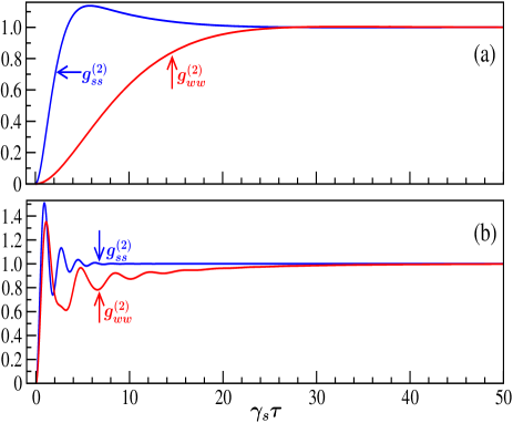
Figure 2: Intensity-intensity correlations $g_{ss}^{(2)}(\tau)$ (blue) and $g_{ww}^{(2)}(\tau)$ (red). The parameters used are: $\gamma_{w}=\Omega_{w}=0.1\gamma_{s}$, $\Delta_{s}=\Delta_{w}=0$, and (a) $\Omega_{s}=0.5\gamma_{s}$, (b) $\Omega_{s}=3.5\gamma_{s}$.

Figure 2 shows intensity correlations when the Rabi frequency of the weak transition is fixed at a value above saturation, $\Omega_{w}=\gamma_{w}$, and the strong transition is driven either moderately, Fig. 2(a), or strongly, Fig. 2(b). For instance, there is the well-known nonclassical feature of antibunching: the atom cannot emit two photons simultaneously, $g^{(2)}(0)=0$ CaWa76 ; KiMa76 . More generally, $g^{(2)}(\tau)<1$ means that the atom is in the nonclassical state of antibunching. For the V3LA we observe this feature because the two transitions feed from the common ground state. However, there are notable differences in their evolution not observed in Ref. PeLK86 .

In Fig. 2(a) $\Omega_{s}/\gamma_{s}=0.5$ and $\Omega_{w}/\gamma_{w}=1$, that is, the weak transition is apparently more strongly driven but its net emission rate $\gamma_{w}\alpha_{ww}$ is smaller than that of the strong transition $\gamma_{s}\alpha_{ss}$. The strong transition (the one with larger $\gamma_{s}$) competes advantageously for transition probability with the weak transition; the average separation among photons in the strong transition is shorter than that for the weak transition. This explains the longer approach towards the value $g_{ww}^{(2)}=1$, which characterizes independent photon emissions.

In Fig. 2(b) we have $\Omega_{s}/\gamma_{s}=3.5$ and $\Omega_{w}/\gamma_{w}=1$. For the strong transition the transient period of $g_{ss}^{(2)}$ shows oscillations at a frequency near $\Omega_{s}$, damped at the approximate rate $3\gamma_{s}/4$, just as it occurs for a two-level atom CaWa76 ; KiMa76 . The dressing of the strong transition, see Fig. 1(b), forces the dynamics of the weak one to evolve at a frequency $\sim\Omega_{s}/2$. Interestingly and unusually, the oscillation regime of $g_{ww}^{(2)}$ occurs mostly below unity, with a long term decay at the rate $\gamma_{w}$, more clearly manifested than in the case of $g_{ss}^{(2)}$. The weak transition is thus in a highly nonclassical state, which certainly calls for a deeper study, such as of its phase-dependent fluctuations.

IV Amplitude-Intensity Correlation

We study the AIC via conditional homodyne detection, see Fig. 3. In this method, the amplitude of a quadrature of the emitted field, $E_{\phi}\propto\sigma_{\phi}=(\sigma_{eg}e^{-i\phi}+\sigma_{ge}e^{i\phi})/2$, for the local oscillator (LO) phase $\phi$, is measured by balanced homodyne detection (BHD) on the condition that the fluorescence intensity $I\propto\sigma_{ee}$ is measured at the detector $\mathrm{D}_{I}$. Assuming stationary dynamics, the normalized AIC function takes the following form

$$h_{\phi}(\tau)=\frac{\langle:\sigma_{eg}(0)\sigma_{ge}(0)\sigma_{\phi}(\tau):\rangle}{\alpha_{ee}\alpha_{\phi}}\,,$$ (3)

where the steady state values of the intensity and the dipole quadrature amplitude are $\alpha_{ee}$ and $\alpha_{\phi}=\langle\sigma_{\phi}\rangle_{st}$, respectively, and the dots $::$ indicate normal and time operator ordering. For positive and negative time intervals we have

$$h_{\phi}(\tau\geq 0) = \frac{\langle\sigma_{eg}(0)\sigma_{\phi}(\tau)\sigma_{ge}(0)\rangle}{\alpha_{ee}\alpha_{\phi}}\,,$$ (4a)

$$h_{\phi}(\tau\leq 0) = \frac{\mathrm{Re}\left[e^{-i\phi}\langle\sigma_{eg}(0)\sigma_{ee}(-\tau)\rangle\right]}{\alpha_{ee}\alpha_{\phi}}\,.$$ (4b)

For $\tau\geq 0$ a photon is detected at $\tau=0$, triggering the detection of a quadrature by balanced homodyne detection. For $\tau\leq 0$, on the other hand, it is the photon detection that follows the quadrature detection. Since the amplitude and intensity operators do not commute, there is no guarantee for symmetry to hold, that is, $h_{\phi}(-\tau)\neq h_{\phi}(\tau)$. The asymmetry results from the different fluctuations of the light’s amplitude and intensity thanks to the breakdown of detailed balance in this system DeCC02 .

Figure 3: Sketch of a conditional homodyne detection setup. See main text for details. The excitation is bichromatic but the local oscillator’s frequency is only that of the observed transition.

We address this issue by analyzing noise properties of the fluorescence. We split the atomic operator dynamics into its mean plus fluctuations, $\sigma_{jk}=\alpha_{jk}+\Delta\sigma_{jk}$, where $\langle\Delta\sigma_{jk}\rangle=0$. The AIC correlation (3) is split as hmcb10

$$h_{\phi}(\tau)=1+h_{\phi}^{(2)}(\tau)+h_{\phi}^{(3)}(\tau)\,,$$ (5)

where $h_{\phi}^{(2)}(\tau)$ and $h_{\phi}^{(3)}(\tau)$ are terms of second and third-order dipole fluctuations $\Delta\sigma_{jk}$ . For positive time intervals between photon and quadrature detection we have

$$h_{\phi}^{(2)}(\tau\geq 0) = \frac{2\mathrm{Re}[\alpha_{ge}\langle\Delta\sigma_{eg}(0)\Delta\sigma_{\phi}(\tau)\rangle]}{\alpha_{ee}\alpha_{\phi}}\,,$$ (6a)

$$h_{\phi}^{(3)}(\tau\geq 0) = \frac{\langle\Delta\sigma_{eg}(0)\Delta\sigma_{\phi}(\tau)\Delta\sigma_{ge}(0)\rangle}{\alpha_{ee}\alpha_{\phi}}\,,$$ (6b)

where $\Delta\sigma_{\phi}=(\Delta\sigma_{eg}e^{-i\phi}+\Delta\sigma_{ge}e^{i\phi})/2$ is the dipole quadrature fluctuation operator. For negative intervals, for which we reinforce notation with the superscript $(N)$, we have

$$h_{\phi}^{(N)}(\tau\leq 0)=1+\frac{\mathrm{Re}[e^{-i\phi}\langle\Delta\sigma_{eg}(0)\Delta\sigma_{ee}(-\tau)\rangle]}{\alpha_{ee}\alpha_{\phi}}\,.$$ (7)

This correlation is only of second-order in the dipole fluctuations. This differs from Eq. (6a), however, by the presence of the time-dependent population noise operator $\Delta\sigma_{ee}$ instead of the time-dependent coherence fluctuation operators $\Delta\sigma_{eg}$ and $\Delta\sigma_{ge}$.

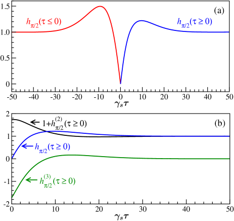
Figure 4: (a) Time-asymmetric AIC of light from the weak transition, for $\phi=\pi/2$. (b) Decomposition of $h_{\pi/2}(\tau\geq 0)$ (blue) into $1+h_{\pi/2}^{(2)}$ (black) and $h_{\pi/2}^{(3)}$ (green). The parameters used are: $\Omega_{s}=0.5\gamma_{s}$, $\Omega_{w}=\gamma_{w}=0.1\gamma_{s}$, $\Delta_{s}=\Delta_{w}=0$.

Figures 4 and 5 show the AIC of the $\phi=\pi/2$ quadrature of the light from the weak transition for $\gamma_{w}=0.1\gamma_{s}$. In Fig. 4 the Rabi frequency for the fast-decaying transition is moderately strong, $\Omega_{s}=0.5\gamma_{s}$, and the Rabi frequency for the weak transition is $\Omega_{w}=0.1\gamma_{s}$ (strong relative to $\gamma_{w}$). In Fig. 4(a) the time asymmetry is evident. Fig. 4(b) shows the AIC decomposition for $\tau\geq 0$ where the second and third-order terms have similar size; this is a signature of a large deviation from Gaussian fluctuations.

Figure 5 shows the effect of the strong transition driven high above saturation, $\Omega_{s}=3.5\gamma_{s}$. In Figure 5(a) the asymmetry is still very clear and its size is increased compared to Fig. 4 due to the smaller values of $\alpha_{ww}$ and $\alpha_{\pi/2}$ used for the normalization; they are smaller because the system is in the regime of large quantum fluctuations due to the dressing of the ground state by the driving on the strong transition which detunes the weak transition laser by $\Omega_{s}/2$. As seen in the $g_{ww}^{(2)}$ photon correlation of Fig. 2(b), and in the frequency spectrum of Fig. 7, these are the dominant frequencies of oscillations of $h_{\pi/2}(\tau)$ of the weak transition. There is a fast decay at $\sim 3\gamma_{s}/4$, while the slow decay due to $\gamma_{w}$ can be seen only for long negative intervals. Figure 5(b) shows the dominance of the third-order term, $h_{\pi/2}(\tau\geq 0)\approx h_{\pi/2}^{(3)}(\tau\geq 0)$, that gives a strong signature of nonlinearity in the weak transition for $\Omega_{w}=\gamma_{w}$. It can be seen how well $h_{\pi/2}^{(3)}(\tau\geq 0)$ compares in size to $h_{\pi/2}^{(N)}(\tau\leq 0)$, which reflect population fluctuations.

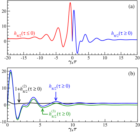
Figure 5: Same as in Fig. 4 except for the stronger driving of the strong transition, with $\Omega_{s}=3.5\gamma_{s}$.

A comment regarding the AIC for the strong transition is in order, but it is not essential to show graphics here. It strongly resembles the cases of the two-level atom hmcb10 and of a different 3LA system CaRG16 . There is asymmetry, but very slight, and occurs in only two regimes: 1) just above saturation, $\Omega_{s}/\gamma_{s}\sim 1/4$, and 2) when the strong laser is detuned a few $\gamma_{s}$ from resonance. In the former the correlation looks like a more symmetric version of Fig. 4. This is approximately the case in the AIC measurement of Ref. GRS+09 for the strong transition of a $\Lambda$-type 3LA. In the latter the asymmetry is noticed only for long correlation time intervals, near the end of oscillations, as seen in Fig. 3(b) of Ref. MaCa08 . In this case experimental background noise may hide the asymmetry.

The AIC provides a strong assessment of the quantum nature of the emitted field through the violation of the classical inequalities CCFO00 ; FOCC00 :

$$0 \leq h_{\phi}(\tau)-1\leq 1\,,$$ (8a)

$$|h_{\phi}(\tau)-1| \leq |h_{\phi}(0)-1|\leq 1\,.$$ (8b)

Clearly, the AIC shown in Figs. 4 and 5 break several of these inequalities MaCa08 ; hmcb10 ; CaGH15 . One of them results from $h_{\pi/2}(0)=0$, which shows the emitted light’s antibunching behavior; there is no field emitted when the atom is in the ground state. Thus, for short intervals $\tau$ the AIC is nonclassical. The other case is concerned with how large this correlation is by exceeding the classical bounds by orders of magnitude, as shown in Fig. 5, due to the small denominator in Eq. 3. Its origin lies in the low photon emission rate that places the system in the regime of large quantum fluctuations.

As shown in Refs. CCFO00 ; FOCC00 , the above classical bounds are stronger criteria for nonclassicality of the emitted field than squeezed light measurements, which provide a more familiar standard for probing phase-dependent fluctuations. We briefly consider this in the next Section. Detailed discussions on the hierarchy of measures of nonclassicality for higher-order correlation functions are presented in Refs. ScVo05 ; ScVo06 .

We close this Section with a discussion on the AIC for the $\phi=0$ quadrature. For nonzero detuning ($\Delta_{w}\neq 0$) the results are qualitatively similar to those of Figs. 4 and 5 but with a smaller amplitude. However, if $\Delta_{w}=0$, the mean dipole quadrature $\langle\sigma_{0}\rangle_{st}=\alpha_{0}$ vanishes for all times, and so is the AIC (via the quantum regression formula). Thus, in order to have a nonzero signal, the dipole field must be mixed with a coherent offset before entering the detection setup CCFO00 . The resulting correlation, however, has a classical character, where features such as antibunching and the violation of classical inequalities, Eqs. (8), are absent.

V Spectra and Variances of Quadratures

In this Section we analyze noise properties in a quadrature of the emitted light field. The variance and the spectrum of squeezing had been the standard measures of quadrature fluctuations, hence it is convenient to include them in our analysis. More precisely, they are a natural part of the study of the AIC in the spectral domain CCFO00 ; FOCC00 ; hmcb10 ; CaGH15 ; CaRG16 . The AIC asymmetry and the large role of third-order fluctuations in resonance fluorescence clearly make the second-order correlation measurements for squeezing insufficient to explore most of the non-classical features of this and other quantum systems.

V.1 Spectral Fluctuations

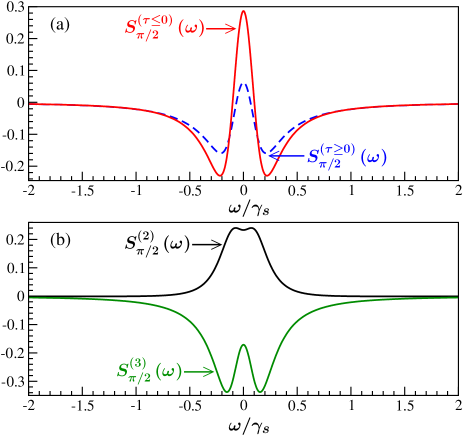
Figure 6: (a) Spectra, Eqs. 9(a,b), for $\phi=\pi/2$ of the AIC of the weak transition plotted in Fig. 4(a). (b) Decomposition of $S_{\pi/2}^{(\tau\geq 0)}$ into its terms of second and third order, Eqs. 9(c). The parameters are: $\Omega_{s}=0.5\gamma_{s}$, $\Omega_{w}=\gamma_{w}=0.1\gamma_{s}$, $\Delta_{s}=\Delta_{w}=0$.

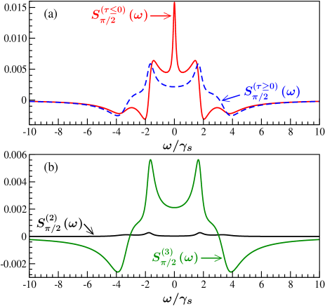
Figure 7: (a) Spectra, Eqs. 9(a,b), for $\phi=\pi/2$ of the AIC of the weak transition plotted in Fig. 5(a). (b) Decomposition of $S_{\pi/2}^{(\tau\geq 0)}$ into its terms of second and third order, Eqs. 9(c). The parameters are: $\Omega_{s}=3.5\gamma_{s}$, $\Omega_{w}=\gamma_{w}=0.1\gamma_{s}$, $\Delta_{s}=\Delta_{w}=0$.

The spectral representation of fluctuations in the AIC provides complementary system information such as oscillation frequencies and decay rates and allows direct comparisons with measures of squeezed light. For the particular problem in this paper, the asymmetry of $h_{\phi}(\tau)$ would suggest the use of the Fourier exponential transform, $\int_{-\infty}^{\infty}\left[h_{\phi}(\tau)-1\right]e^{i\omega\tau}\,d\tau$. However, the fact that the AIC carries different information for positive and negative time intervals $\tau$, spectra should be obtained separately by the Fourier cosine transform,

$$S_{\phi}^{(\tau\leq 0)}(\omega) = 4\gamma_{e}\alpha_{ee}\int_{0}^{\infty}\left[h_{\phi}(\tau\leq 0)-1\right]\cos{\omega\tau}\,d\tau\,,$$ (9a)

$$S_{\phi}^{(\tau\geq 0)}(\omega) = 4\gamma_{e}\alpha_{ee}\int_{0}^{\infty}\left[h_{\phi}(\tau\geq 0)-1\right]\cos{\omega\tau}\,d\tau\,,$$ (9b)

$$= S_{\phi}^{(2)}(\omega)+S_{\phi}^{(3)}(\omega)\,,$$ (9c)

where we took into account the splitting of $h_{\phi}(\tau\geq 0)$ into its second- and third-order terms. A Fourier exponential transform would only average the spectra of both sides of $h_{\phi}(\tau)$, so incorrect information would be given.

A signature of squeezed light is represented by the negative values of the frequency spectral function. Likewise, negative values in the AIC spectra indicate nonclassical light, beyond squeezing. It has been shown that the so-called spectrum of squeezing CoWZ84 ; RiCa88 and the second-order spectrum are related as $S_{\phi}^{sq}(\omega)=\eta S_{\phi}^{(2)}(\omega)$ CCFO00 ; FOCC00 , where $\eta$ is a combined collection and detection efficiency. The AIC, due to its conditional detection nature, is independent of this $\eta$ factor.

Figure 6 shows the spectra of the AIC of Fig. 4, with the strong transition excited moderately. The spectrum $S_{\pi/2}^{(\tau\geq 0)}(\omega)$ has a large central peak over a broad negative feature that reveals nonclassical features of the emitted light. Its decomposition, Fig. 6(b), shows that there is no squeezing, $S_{\pi/2}^{(2)}(\omega)\geq 0$, but a fully nonclassical (negative) bimodal feature is present in the third-order spectrum. The peaks are located around $\omega=\pm\Omega_{s}/2=\pm 0.25\gamma_{s}$. The spectrum $S_{\pi/2}^{(\tau\leq 0)}$ has a larger central peak, which reflects the larger amplitude of $h_{\pi/2}(\tau\leq 0)$. In both cases, the fact that the spectra have negative values reflects the presence of nonclassical effects such as antibunching and large fluctuations that lead to the violation of the inequalities in Eq. (8).

A stronger excitation of the $|g\rangle-|s\rangle$ transition makes it easier to extract spectral and transition dynamic information. Figure 7 gives the spectra of the AIC presented in Fig. 5. The peaks near $\pm\Omega_{s}/2\,(\simeq\pm 1.75)$, due to the dressing of the strong transition, are reminiscent of the Autler-Townes effect, with slightly different splittings. For $S_{\pi/2}^{(\tau\leq 0)}$ in Fig. 7(a), there is the outstanding feature of a narrow central peak, which reflects the slow decay at the rate $\gamma_{w}$, a remnant of electron shelving in the system CaRG16 . Such narrow peak is absent in $S_{\pi/2}^{(\tau\geq 0)}$, that is, there is no slow decay of $h_{\pi/2}(\tau\geq 0)$. The spectra $S_{\pi/2}^{(\tau\geq 0)}$ and $S_{\pi/2}^{(\tau\leq 0)}$ have a strong dispersive component because of the nonlinearity induced by driving the transition $|g\rangle-|w\rangle$ high above saturation. Fig. 7(b) clearly shows the dominance of the third-order fluctuations hmcb10 .

Figure 8: (a) Variance of fluorescence of the strong transition for $\phi=\pi/2$. The parameters used are: i) $\gamma_{w}=0.01\gamma_{s}$, $\Omega_{w}=0.05\gamma_{s}$, ii) $\gamma_{w}=0.01\gamma_{s}$, $\Omega_{w}=0.1\gamma_{s}$, iii) $\gamma_{w}=0.1\gamma_{s}$, $\Omega_{w}=0.1\gamma_{s}$. (b) Variance of fluorescence of the weak transition for $\phi=\pi/2$, $\gamma_{w}=0.1\gamma_{s}$, and: i) $\Omega_{s}=0.1\gamma_{s}$, ii) $\Omega_{s}=0.2\gamma_{s}$, iii) $\Omega_{s}=0.5\gamma_{s}$. For all cases detunings are zero.

V.2 Variance and Total Quadrature Noise

The noise in a quadrature is usually given by the variance

$$V_{\phi}=\langle:(\Delta\sigma_{\phi})^{2}:\rangle=\mathrm{Re}\left[e^{-i\phi}\langle\Delta\sigma_{eg}\Delta\sigma_{\phi}\rangle\right]\,,$$ (10)

which is the unnormalized second-order amplitude-intensity correlation. The variance is related to the integrated spectrum of squeezing as $\int_{-\infty}{\infty}S_{\phi}^{(2)}(\omega)\,d\omega=4\pi\gamma_{e}\eta V_{\phi}$. Negative values of the variance are a signature of squeezed fluctuations. For the strong transition, the squeezing for $\phi=\pi/2$ is small or null, Fig. 8(a), compared to the case of a two-level atom RiCa88 ; CaRG16 ; SHJ+15 . The reduction of squeezing is due to the added incoherent emission in the weak transition. The weak transition also features squeezing, Fig. 8(b), but not much larger than for the strong transition.

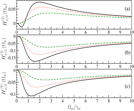
Figure 9: Noise for $\phi=\pi/2$ from CHD of the weak transition in (a) second order, (b) third order for $\tau\geq 0$, and (c) for $\tau\leq 0$. Parameters are: $\gamma_{w}=0.1\gamma_{s}$, $\Omega_{s}=0.1\gamma_{s}$ (solid-black), $\Omega_{s}=0.5\gamma_{s}$ (dotted-red), $\Omega_{s}=0.9\gamma_{s}$ (dashed-green). For all curves detunings are zero.

As for the spectrum of squeezing, the variance is not the right measure of noise for the AIC. It has two problems. The first is the asymmetry itself, which forces us to consider the noise from the positive and the negative time interval parts of the correlation separately. The second is that it is not possible to separate experimentally the second- and third-order terms in the $\tau\geq 0$ part. We have, however, found it useful to perform such separation in order to explain the origin of nonclassical features of the AIC correlation functions. A natural choice to measure the noise is to integrate the spectra of Figs. 6 and 7, which are proportional to the initial values of the unnormalized correlations (6) and (7),

$$H_{\phi}^{(2)} = 2\mathrm{Re}[\alpha_{ge}\langle\Delta\sigma_{eg}\Delta\sigma_{\phi}\rangle]\,,$$ (11a)

$$H_{\phi}^{(3)} = \langle\Delta\sigma_{eg}\Delta\sigma_{\phi}\Delta\sigma_{ge}\rangle\,,$$ (11b)

$$H_{\phi}^{(N)} = \mathrm{Re}[e^{-i\phi}\langle\Delta\sigma_{eg}\Delta\sigma_{ee}\rangle]\,,$$ (11c)

where the noise correlations $\langle\cdots\rangle$ are given in Eqs. (12).

In Fig. 9 we plot such noise functions of the $\phi=\pi/2$ quadrature of the weak transition. Since the variance is proportional to $H_{\phi}^{(2)}$, there is a narrow range of Rabi frequencies $\Omega_{w}$ where the noise is negative [compare line (i) in Fig. 8(b) and solid line in Fig. 9(a)]. Stronger driving in both transitions destroys squeezing. The third-order term is seen to be nonclassical for a wider range of Rabi frequencies, Fig. 9(b), and it is the dominant term of the total noise. Since these noise functions are evaluated at $\tau=0$, we obtain $H_{\phi}^{(N)}(0)=H_{\phi}^{(2)}(0)+H_{\phi}^{(3)}(0)$, which can be readily seen in Fig. 9(c).

VI Conclusions

We have investigated quantum fluctuations of the scattered light from two monochromatically driven transitions of a V-type 3LA, mainly using phase-dependent amplitude-intensity correlations. The noncommutativity of amplitude and intensity operators and the competition among transitions make the correlation asymmetric and large, more pronounced for the weak transition, which has larger quantum fluctuations than the strong one. The asymmetry is a signature of nonclassical and non-Gaussian fluctuations (hence the breakdown of detailed balance) which manifest as different oscillation frequencies and decays in the spectra (and integrated spectra) associated with the positive and negative time intervals of the AIC correlations. Third-order fluctuations, with their dispersive spectral shape, are dominant for strong excitation of a transition. We also showed that the correlation of two photons from the weak transition has enhanced nonclassical behavior of intensity fluctuations: even for strong excitation, the correlation evolves most of the time below the level of a coherent state. CHD is a valuable tool to study the AIC to reveal not only nonclassical states of the field fluctuations but also to explore nonequilibrium physics in microscopic systems.

Appendix

To calculate correlations, spectra, variances, and noise, we evaluate the zero interval, steady state, correlations:

$$\langle\Delta\sigma_{eg}\Delta\sigma_{ge}\rangle = \alpha_{ee}-|\alpha_{eg}|^{2}\,,$$ (12a)

$$\langle\Delta\sigma_{eg}\Delta\sigma_{eg}\rangle = -\alpha_{eg}^{2}\,,$$ (12b)

$$\langle\Delta\sigma_{eg}\Delta\sigma_{ee}\rangle = -\alpha_{eg}\alpha_{ee}\,,$$ (12c)

$$\langle\Delta\sigma_{eg}\Delta\sigma_{ge}\Delta\sigma_{ge}\rangle = 2\alpha_{ge}(|\alpha_{eg}|^{2}-\alpha_{ee})\,,$$ (12d)

$$\langle\Delta\sigma_{eg}\Delta\sigma_{eg}\Delta\sigma_{ge}\rangle = 2\alpha_{eg}(|\alpha_{eg}|^{2}-\alpha_{ee})\,,$$ (12e)

where $\Delta\sigma_{jk}=\sigma_{jk}-\alpha_{jk}$.

Additionally, we observe that $h_{\phi}(0)=0$ (as for antibunching, given the fermionic character of the dipole operators). From Eqs. (6) and (12), we can calculate the third-order AIC correlation for $\tau=0$,

$$h_{\phi}^{(3)}(0)=-\left[1+h_{\phi}^{(2)}(0)\right]=\frac{2(|\alpha_{eg}|^{2}-\alpha_{ee})}{\alpha_{ee}}\,.$$ (13)

For strong driving $h_{\phi}^{(3)}(0)\to-2$, whether it is the strong transition or the weak one. In this regime, the stationary excited state population is bound as $\alpha_{ee}<0.5$, while the coherence is very small, $|\alpha_{eg}|^{2}\sim\Omega_{e}^{-2}\to 0$.

References

- (1) R. Hanbury-Brown and R. Q. Twiss, “Correlation between photons in two coherent beams of light,” Nature 177, 27-29 (1956).
- (2) H. J. Carmichael, H. M. Castro-Beltran, G. T. Foster, and L. A. Orozco, “Giant violations of classical inequalities through conditional homodyne detection of the quadrature amplitudes of light,” Phys. Rev. Lett. 85, 1855-1858 (2000).
- (3) G. T. Foster, L. A. Orozco, H. M. Castro-Beltran, and H. J. Carmichael, “Quantum state reduction and conditional time evolution of wave-particle correlations in cavity QED,” Phys. Rev. Lett. 85, 3149-3152 (2000).
- (4) For a review on CHD see H. J. Carmichael, G. T. Foster, L. A. Orozco, J. E. Reiner, and P. R. Rice, “Intensity-field correlations of non-classical light,” in Progress in Optics 46, E. Wolf, ed. (Elsevier, 2004).
- (5) W. Vogel, “Squeezing and anomalous moments in resonance fluorescence,” Phys. Rev. Lett. 67, 2450-2452 (1991).
- (6) W. Vogel, “Homodyne correlation measurements with weak local oscillators,” Phys. Rev. A 51, 41-60 (1995).
- (7) B. Kühn, W. Vogel, M. Mraz, S. Köhnke, and B. Hage, “Anomalous quantum correlations of squeezed light,” Phys. Rev. Lett. 118, 153601 (2017).
- (8) A. Denisov, H. M. Castro-Beltran, and H. J. Carmichael, “Time-asymmetric fluctuations of light and the breakdown of detailed balance,” Phys. Rev. Lett. 88, 243601 (2002).
- (9) E. R. Marquina-Cruz and H. M. Castro-Beltran, ‘Nonclassicality of resonance fluorescence via amplitude-intensity correlations,” Laser Phys. 18, 157-164 (2008).
- (10) H. M. Castro-Beltrán, L. Gutiérrez, and E. R. Marquina-Cruz, in “Latin America Optics and Photonics, Cancun, Mexico, 2014,” OSA Technical Digest, paper LM4A.38 (Optical Society of America, Washington, D.C. 2014).
- (11) Q. Xu, E. Greplova, B. Julsgaard, and K. Mølmer, “Correlation functions and conditioned quantum dynamics in photodetection theory,” Phys. Scripta 90, 128004 (2015).
- (12) Q. Xu and K. Mølmer, “Intensity and amplitude correlations in the fluorescence from atoms with interacting Rydberg states,” Phys. Rev. A 92, 033830 (2015).
- (13) F. Wang, X. Feng, and C. H. Oh, “Intensity-intensity and intensity-amplitude correlation of microwave photons from a superconducting artificial atom,” Laser Phys. Lett. 13, 105201 (2016).
- (14) H. M. Castro-Beltran, “Phase-dependent fluctuations of resonance fluorescence beyond the squeezing regime,” Optics Commun. 283, 4680-4684 (2010).
- (15) H. M. Castro-Beltran, L. Gutierrez, and L. Horvath, “Squeezed versus non-Gaussian fluctuations in resonance fluorescence,” Appl. Math. Inf. Sci. 9, 2849-2857 (2015).
- (16) H. M. Castro-Beltrán, R. Román-Ancheyta, and L. Gutiérrez, “Phase-dependent fluctuations of intermittent resonance fluorescence,” Phys. Rev. A 93, 033801 (2016).
- (17) S. Gammelmark, B. Julsgaard, and K. Mølmer, “Past quantum states of a monitored system,” Phys. Rev. Lett. 111, 160401 (2013).
- (18) The breakdown of detailed balance in two-level atom resonance fluorescence was demonstrated in D. F. Walls, H. J. Carmichael, R. F. Gragg, and W. C. Schieve, “Detailed balance, Liapounov stability, and entropy in resonance fluorescence,” Phys. Rev. A 18, 1622-1627 (1978).
- (19) M. B. Plenio and P. L. Knight, “The quantum-jump approach to dissipative dynamics in quantum optics,” Rev. Mod. Phys. 70, 101-144 (1997).
- (20) S. H. Autler and C. H. Townes, “Stark effect in rapidly varying fields,” Phys. Rev. 100, 703-722 (1955).
- (21) J. von Zanthier, C. Skornia, G. S. Agarwal, and H. Walther, “Quantum coherence in a single ion due to strong excitation of a metastable transition,” Phys. Rev. A 63, 013816 (2000).
- (22) H. J. Carmichael and D. F. Walls, “A quantum-mechanical master equation treatment of the dynamical Stark effect,” J. Phys. B 9, 1199-1219 (1976).
- (23) H. J. Kimble and L. Mandel, “Theory of resonance fluorescence,” Phys. Rev. A 13, 2123-2144 (1976).
- (24) D. T. Pegg, R. Loudon, and P. L. Knight, “Correlations in light emitted by three-level atoms,” Phys. Rev. A 33, 4085-4091 (1986).
- (25) S. Gerber, D. Rotter, L. Slodička, J. Eschner, H. J. Carmichael, and R. Blatt, “Intensity-field correlation of single-atom resonance fluorescence,” Phys. Rev. Lett. 102, 183601 (2009).
- (26) E. V. Shchukin and W. Vogel, “Nonclassical moments and their measurement,” Phys. Rev. A 72, 043808 (2005).
- (27) E. V. Shchukin and W. Vogel, “Universal measurement of quantum correlations of radiation,” Phys. Rev. Lett. 96, 200403 (2006).
- (28) M. J. Collett, D. F. Walls, P. Zoller, “Spectrum of squeezing in resonance fluorescence,” Optics Commun. 52, 145-149 (1984).
- (29) P. R. Rice and H. J. Carmichael, “Nonclassical effects in optical spectra,” J. Opt. Soc. Am. B 5, 1661-1668 (1988).
- (30) C. H. H. Schulte, J. Hansom, A. E. Jones, C. Matthiesen, C. Le Gall, and M. Atatüre, “Quadrature squeezed photons from a two-level system,” Nature 525, 222-226 (2015).