Discovery of a Synchrotron Bubble Associated with PSR J1015$-$5719

Abstract

We report the discovery of a synchrotron nebula, G283.1$-$0.59, associated with PSR J1015$-$5719. Radio observations using the Molonglo Observatory Synthesis Telescope and the Australia Telescope Compact Array at 36, 16, 6, and 3 cm reveal a complex morphology. The pulsar is embedded in the “head” of the nebula with fan-shaped diffuse emission. This is connected to a circular bubble of 20″ radius and a collimated tail extending over 1′. Polarization measurements show a highly ordered magnetic field in the nebula. It wraps around the edge of the head and shows an azimuthal configuration near the pulsar, then switches direction quasi-periodically near the bubble and in the tail. Together with the flat radio spectrum observed, we suggest that this system is most plausibly a pulsar wind nebula (PWN), with the head as a bow shock that has a low Mach number and the bubble as a shell expanding in a dense environment. The bubble could act as a magnetic bottle trapping the relativistic particles. A comparison with other bow-shock PWNe with higher Mach numbers shows similar structure and $B$-field geometry, implying that pulsar velocity may not be the most critical factor in determining the properties of these systems.

We also derive analytic expressions for the projected standoff distance and shape of an inclined bow shock. It is found that the projected distance is always larger than the true distance in three dimensions. On the other hand, the projected shape is not sensitive to the inclination after rescaling with the projected standoff distance.

1. Introduction

As a pulsar spins down, most of its rotational energy is carried away by a relativistic particle and magnetic field outflows known as a pulsar wind. The interaction of the wind with the ambient medium results in a pulsar wind nebula (PWN), emitting broadband synchrotron radiation from radio to X-ray bands. As an aged pulsar generally travels in the interstellar medium (ISM) faster than the local sound speed, the wind is confined by the ram pressure, giving rise to a bow-shock PWN. There are over a dozen of such systems known and most of them are moving at a high Mach number (see Kargaltsev & Pavlov, 2008). They are characterized by a long collimated tail with a small bow-shock standoff distance, which makes them easier to identify than low-velocity examples.

While bow shocks are governed by simple boundary conditions, they exhibit diverse properties. Observations reveal a peculiar structure with a bubble or a central bulge (e.g. Cordes et al., 1993; Ng et al., 2010) and different magnetic field geometry (e.g., Yusef-Zadeh & Gaensler, 2005; Ng et al., 2010, 2012). The exact origin of these features remains unclear. It could be related to the pulsar age, velocity, flow condition of the wind, the relative orientation of the pulsar spin, etc. To identify which factor plays a critical role, it is essential to expand the sample. We present here the discovery of a new bow-shock PWN, G283.1$-$0.59 (catalog ), associated with PSR J1015$-$5719 (catalog ) (hereafter, J1015). As we argue, this is an unusual system traveling at a low Mach number and showing many remarkable properties, thus offering an important example for understanding bow shocks.

Table 1Radio Observations of J1015 Used in This Study

Obs. Date	Array	Wavelength	Center Freq.	No. of	Usable Band-	Integration
	Config.	(cm)	(MHz)	Channels	width (MHz)	Time (hr)
MOST
2008 Apr 6, 13, 19, 20	$\cdots$	36	843	1	3	48
ATCA
2008 Dec 13	750B	6, 3	4800, 8640	13	104	12.5
2009 Feb 17	EW352	6, 3	4800, 8640	13	104	12.5
2009 Aug 2	1.5A	6, 3	5500, 9000	2048	1848	11.5
2010 Feb 5	6A	6, 3	5500, 9000	2048	1848	10
2011 Nov 17	1.5D	16	2100, 2102	2048, 256	1848	1

The MOST data reduction followed the custom procedure outlined in Bock et al. (1999) and Green et al. (1999). We first removed those data samples most strongly affected by radio frequency interference (RFI), then calibrated the pointing and flux density scale using sources listed in Campbell-Wilson & Hunstead (1994). Finally, we formed an intensity map and performed deconvolution with a CLEAN algorithm (Högbom, 1974). This was straightforward because of the nearly continuous $u$–$v$ coverage of the MOST observation. The final radio image at 843 MHz was formed using the task IMCOMB in MIRIAD (Sault et al., 1995) to co-add the four separate images; the beam size was $43\arcsec\times 51\arcsec$ FWHM and the rms noise in regions away from the diffuse emission was $\sim 2$ mJy beam^-1.

J1015 is an energetic pulsar discovered in the Parkes Multibeam Pulsar Survey (Kramer et al., 2003). It has spin period $P=0.14$ s, spin-down luminosity $\dot{E}=8.3\times 10^{35}$ erg s^-1, and characteristic age $\tau_{c}=39$ kyr. The dispersion measure (DM) gives a distance estimate of 5.1 kpc (Cordes & Lazio, 2002). Johnston & Weisberg (2006) performed polarization measurements of the pulsar, and found that the swing of the position angle (PA) across phase can be well fitted by the rotating vector model. They inferred a PA of 62° (north through east) for the projected pulsar spin axis on the plane of the sky. The pulsar is located near the gamma-ray source 3EG J1014$-$5705 detected with EGRET. Although an association had been suggested (Torres et al., 2001), recent Fermi LAT observations identified the gamma-ray source as 3FGL J1013.6$-$5734 and the refined position is over 20′ from J1015 (Acero et al., 2015). J1015 now lies beyond the 95% error ellipse of the gamma-ray position, making the association unlikely. So far there is no detection of pulsed or persistent gamma-ray emission at the pulsar position. Infrared, optical, and X-ray observations also found no counterparts (Wang et al., 2014).

A radio image of the field from the second epoch Molonglo Galactic Plane Survey (MGPS2; Murphy et al., 2007; Green et al., 2014) shows extended emission near J1015 at 36 cm. In this study we present deeper radio observations with the Molonglo Observatory Synthesis Telescope (MOST), and higher-resolution observations taken with the Australia Telescope Compact Array (ATCA). The observations and data reduction are described in Section 2. The results are reported in Section 3 and are discussed in Section 4. We summarize the findings in Section 5. Finally, we derive analytic expressions of the projected standoff distance and shape of an inclined bow shock in Appendix A, and we present an evolution model of a bubble with continuous energy injection in a uniform medium in Appendix B. The new images resolved the extended emission and revealed a bubble-like structure, with a high degree of linear polarization and a flat spectrum. We suggest that this is a newly identified bow-shock PWN associated with J1015.

2. Observations and Data Reduction

Radio continuum observations of the field of J1015 were made with MOST and ATCA, and the details are listed in Table 1. MOST operated at a wavelength of 36 cm with a bandwidth of 3 MHz, and it only recorded the right-hand circular polarization. For ATCA, J1015 was observed at 3 and 6 cm with a 4-pointing mosaic in different array configurations. Two early observations had a useful bandwidth of $\sim$100 MHz, and two later ones were taken after the compact array broadband backend upgrade (Wilson et al., 2011), which provided a much larger bandwidth of 2 GHz. Further data obtained on 2009 August 8 were not usable due to an instrumental problem. At 16 cm, the ATCA observation was part of a snapshot survey, and the total integration time on J1015 was 1 hr spread over 12 hr. It was done simultaneously in both the standard observing mode and the pulsar binning mode. The latter provided a high time resolution and the pulse period of J1015 was divided into 32 phase bins to measure the pulse profile and to form on- and off-pulsed images. All ATCA data had full Stokes parameters recorded. PKS B1934$-$638 was used as the flux and bandpass calibrator. PKS B1036$-$52 was used as the phase calibrator at 3 and 6 cm, while PKS B1049$-$53 was used at 16 cm.

We carried out the ATCA data reduction and analysis using MIRIAD. We first removed edge channels and flagged bad visibility data points affected by RFI, then employed the standard procedure to determine and apply the bandpass, gain, flux, and polarization calibration corrections. The 3 and 6 cm images were formed with natural weighting, multifrequency synthesis, and a Gaussian taper of FWHM 4″ to boost the signal-to-noise ratio (S/N). We deconvolved the mosaicked images in Stokes I, Q, and U jointly using a maximum entropy algorithm (PMOSMEM; Sault et al., 1999) and restored them with a circular Gaussian beam of FWHM 4″. The final 3 and 6 cm maps had rms noise of 20 $\mu$Jy beam^-1 and 15 $\mu$Jy beam^-1, respectively, consistent with the theoretical values.

For the 16 cm observation, we applied the same flagging and calibration procedures as above. The pulsar binning data were corrected for dispersion using the DM value for J1015. Since the fractional bandwidth is very large, we divided the data into eight bands of 256 MHz to form separate images. The Briggs (1995) weighting scheme was employed with the robust parameter of 0.5, which optimizes the weighting between resolution and noise level. Images were deconvolved using the CLEAN algorithm and restored with a gaussian beam. The results were combined to form final images in Stokes I, Q, and U. After averaging, the center frequency was 2.2 GHz and the images had beams of FWHM $8\arcsec\times 7\arcsec$ and rms noise of 50 $\mu$Jy beam^-1.

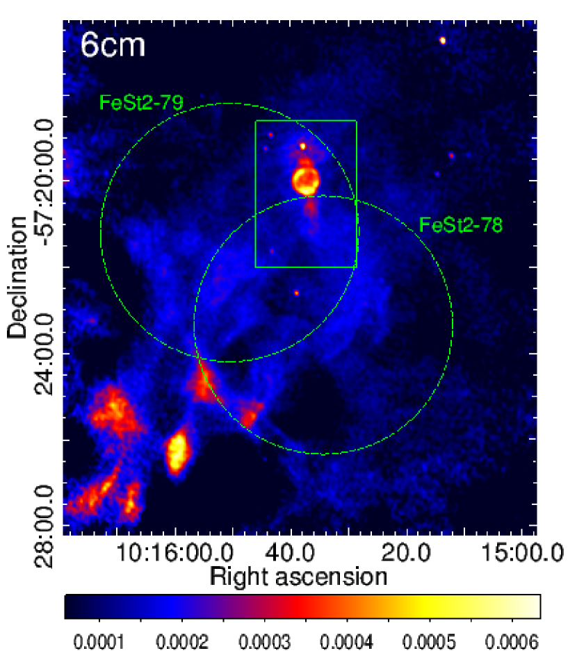
Figure 1.— Radio intensity maps of the field of J1015 at 36 and 6 cm taken with MOST and ATCA, respectively. In the MOST image, the cross marks the pulsar position and the beam size is shown in the lower left. In the ATCA image, the dashed circles indicate the location of two optical dust clouds, FeSt2-78 and FeSt2-79 (Feitzinger & Stuewe, 1984; Dutra & Bica, 2002). The circle diameters of 6′ illustrate the resolution of the optical survey and the actual extents of the clouds are likely smaller. The boxes show the field of view of Figure 2. The color bars are in units of Jy beam^-1.

3. Results

3.1. Morphology

Figure 1 shows the radio intensity maps of the field of J1015. The MOST 36 cm image indicates a compact nebula, which we designate G283.1$-$0.59, extending $\sim$2$\farcm$5 south from the pulsar position. Further southeast, there is large-scale diffuse emission over 4′ in size. The compact nebula is resolved by the higher-resolution ATCA images at 16, 6, and 3 cm in Figure 2, revealing a complex morphology. J1015 is detected in all the bands. It is surrounded by faint fan-shaped emission that we refer to as the “head” of the nebula. The head is $\sim$1$\farcm$5 wide and its apex is 20″ north of the pulsar. It connects to a circular bubble-like structure in the south. The latter has a radius of 20″ and the center is $\sim$50″ away from the pulsar. Beyond the bubble, there is a faint collimated tail extending 1′ further south, such that the entire nebula elongates in the north–south direction with a PA of $\sim$185°.

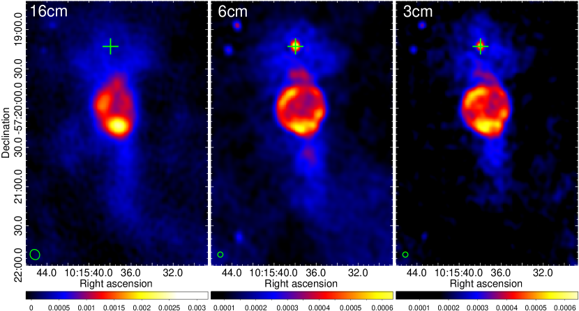
Figure 2.— ATCA radio intensity maps zoomed in at J1015 and the nebula G283.1$-$0.59 at 16, 6, and 3 cm. The 16 cm image is obtained from the off-pulse phase bins with the pulsar binning data (see Figure 4 for the pulse profile of J1015.) The crosses mark the pulsar position and the beam sizes are shown in the lower left. The color bars are in units of Jy beam^-1.

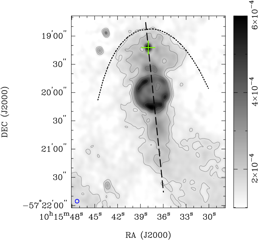
Figure 3.— The same 6 cm intensity map of J1015 and G283.1$-$0.59 as in Figure 2, overlaid with intensity contours at levels of 0.15, 0.2, 0.35, and 0.5 mJy beam^-1. The dotted curve shows a theoretical model of a classical bow shock (Wilkin, 1996) and the dashed line indicates its axis of symmetry. The cross marks the pulsar position and the beam size is shown in the lower left. The gray scale is linear and the color bar is in units of Jy beam^-1.

The morphology of the head resembles the shape of a classical bow shock. We therefore compared the image with a theoretical model given by Wilkin (1996). The result is plotted in Figure 3, which indicates a very good match and suggests a projected stand-off distance of $\sim$20″. The bubble exhibits a similar morphology in all ATCA images and is much brighter around the rim than in the interior. The emission peaks in the south and northeast rim with comparable flux density at 6 and 3 cm, while the northeast rim is fainter than the south one at 16 cm. The bright emission at the south rim seems to extend further to the southwest in the 6 and 3 cm images, although less obvious at 16 cm.

We examined the infrared, optical, and X-ray images of the field using the same data as in Wang et al. (2014), but found no counterparts of G283.1$-$0.59. There are two optical dark clouds, FeSt2-78 and FeSt2-79 (Feitzinger & Stuewe, 1984) overlapping with the nebula. Their locations are shown in Figure 1 and their reported sizes are no larger than the survey resolution of 6′ (Dutra & Bica, 2002). We attempted to identify the clouds in CO and H i surveys (Dame et al., 2001; Ben Bekhti et al., 2016), but the resolution of these radio maps was too low to be useful. Finally, in Figure 4 we plot the pulse profile of J1015 obtained from the 16 cm pulsar binning data. It exhibits a double peak feature similar to that at 21 cm (Johnston & Weisberg, 2006), while the two peaks have comparable intensity. Using the off-pulse data between phase 0.11 and 0.70, we formed an intensity map of the nebula and it is shown in Figure 2.

Figure 4.— Pulse profile of J1015 obtained with the 16 cm pulsar binning observation. Two cycles are plotted and the shaded and unshaded regions denote the on- and off-pulse phases, respectively, chosen for the pulsed flux density measurement. An image formed with the off-pulse phase is shown in Figure 2.

3.2. Spectroscopy

We estimated the flux densities of G283.1$-$0.59 from our radio maps and the Southern Galactic Plane Survey (SGPS; Haverkorn et al., 2006) 21 cm image. The lower-resolution MOST and SGPS images only allow us to measure the total flux density of the entire nebula including the pulsar, while the higher-resolution ATCA maps provide flux density measurements of different regions. At 16 cm we obtained the nebula flux density from the standard mode observation since it has more channels than the pulsar binning data, thus better rejects the RFI and gives a higher S/N image. The pulsar binning data were used to measure the pulsar flux density, by subtracting the off-pulsed data from the on-pulsed ones using the MIRIAD task psrbl (see Figure 4 for the definition of the phase ranges). All results are listed in Table 2 and plotted in Figure 5. The uncertainties are mostly due to strong variations of the background. We also list the pulsar flux density measured with single-dish observations for comparison. Note that the updated value of 3.5 mJy at 21 cm (Johnston & Weisberg, 2006) is adopted here, instead of $0.9\pm 0.1$ mJy reported in the discovery paper (Kramer et al., 2003).

The spectral indices of different regions are determined from simple fits with a power law $S_{\nu}\propto\nu^{\alpha}$. The overall spectrum of the nebula plus pulsar is rather flat with an index $\alpha=-0.3$, while that of the pulsar is much steeper ($\alpha=-1.04$) and that of the bubble is flatter ($\alpha=-0.13$). The south rim exhibits a steeper spectrum than the northeast one ($\alpha=-0.24$ vs. $-0.10$). The head and tail generally show flat spectra, albeit with large uncertainties since these features are faint. We attempted to generate a spectral map of the field, but the S/N was too low to be useful.

Table 2Background-subtracted Flux Densities and Best-fit Spectral Indices of Different Regions in G283.1$-$0.59

Region		Flux Density (mJy)									Spectral Index
		36 cm	20 cm	16 cm		6 cm		3 cm
All (pulsar+PWN)		$110\pm 30$	$90\pm 20$	65$\pm$	10	65$\pm$	10	45$\pm$	6		$-0.3$$\pm$	0.1
Pulsar		$\cdots$	3.5	2.00$\pm$	0.05	1.0$\pm$	0.1	0.6$\pm$	0.1		$-1.04$$\pm$	0.04
Bubble		$\cdots$	$\cdots$	28$\pm$	2	26.5$\pm$	1	23.5$\pm$	1		$-0.13$$\pm$	0.06
Head (excl. pulsar)		$\cdots$	$\cdots$	16$\pm$	3	16$\pm$	2	15$\pm$	2		0.0$\pm$	0.2
Tail		$\cdots$	$\cdots$	9$\pm$	2	8$\pm$	2	6$\pm$	2		$-0.2$$\pm$	0.3
Bubble northeast rim		$\cdots$	$\cdots$	5.8$\pm$	0.3	5.5$\pm$	0.2	5.0$\pm$	0.2		$-0.10$$\pm$	0.05
Bubble south rim		$\cdots$	$\cdots$	6.5$\pm$	0.2	5.4$\pm$	0.2	4.6$\pm$	0.2		$-0.24$$\pm$	0.04

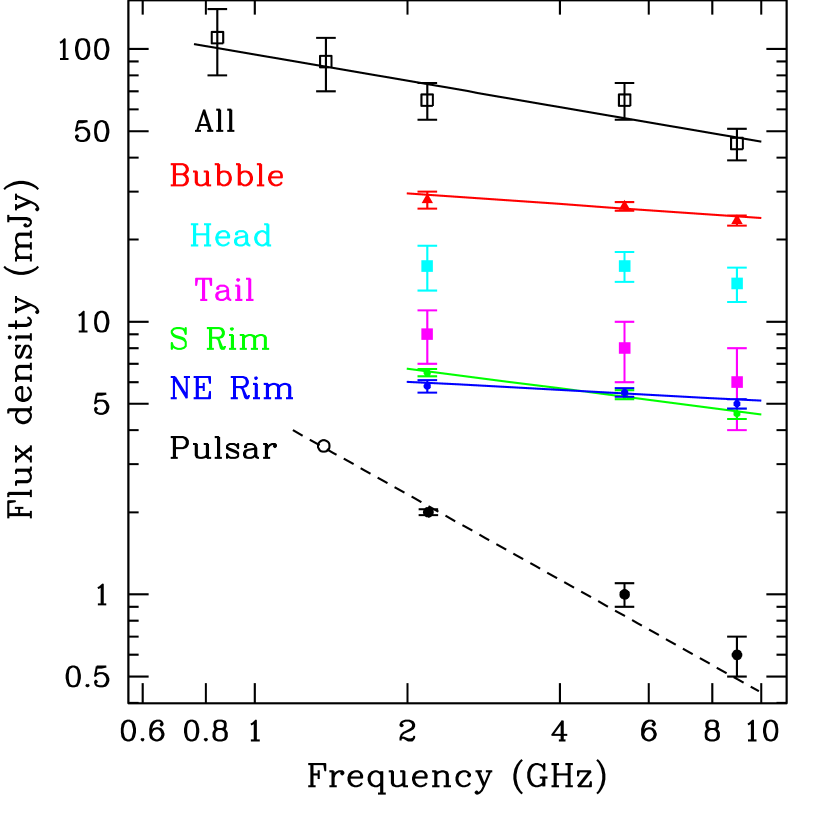
Figure 5.— Radio spectrum of J1015 and different regions of G283.1$-$0.59 as listed in Table 2. The open circle is the pulsed flux obtained with single-dish observations (Johnston & Weisberg, 2006). We do not show the fits for the head and tail here due to the large uncertainties.

3.3. Polarimetry

Figure 6 shows the 6 and 3 cm linearly polarized intensity maps. The emission of G283.1$-$0.59 is highly polarized, and the polarized flux generally follows the total intensity, except it is enhanced near the bubble center and rather faint in the west rim of the bubble. The fractional polarization of the nebula is over 30% in both bands. In particular, it is $\sim$50% at the bubble center and $\sim$30% near the rim. The large-scale diffuse emission in the southeast (see Figure 1) is unpolarized, hence it could be background emission unrelated to the nebula. We do not show the 16 cm result, since only a very low degree of polarization was found. This can be attributed to beam depolarization due to rapid variation in rotation measure (RM) across the field (see below).

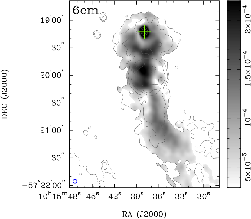
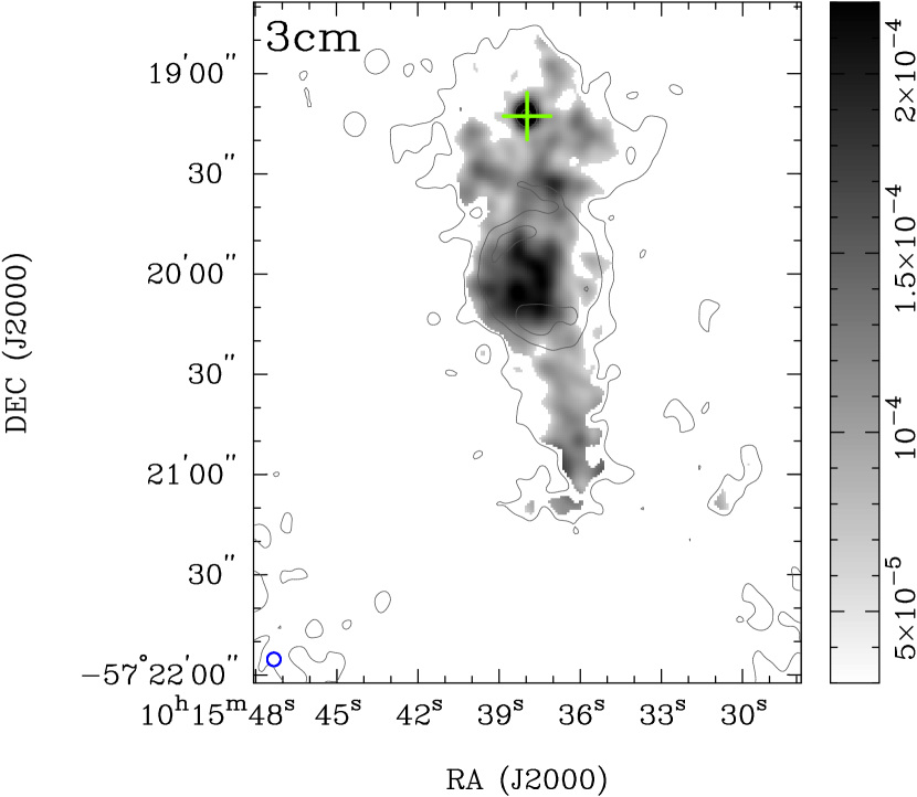
Figure 6.— Linearly polarized intensity of G283.1$-$0.59 at 3 and 6 cm, overlaid with total intensity contours at levels of 0.15, 0.2, 0.35, and 0.5 mJy beam^-1. The maps are clipped where the polarized intensity has S/N$<3$ or the total intensity has S/N$<10$. The gray scales are linear, ranging from 0.03 to 0.22 mJy beam^-1 The crosses mark the pulsar position and the beam sizes are shown in the lower left.

We estimated the foreground RM by comparing the polarization angles at 3 and 6 cm, and the result is shown in Figure 7. The RM changes significantly across the nebula, from $\sim$100 rad m^-2 in the head to $\sim$300 rad m^-2 near the bubble. It then drops rapidly to 0 rad m^-2 in the tail. We found RM$\sim$100 rad m^-2 near the pulsar, consistent with the previously reported value of $96\pm 2$ rad m^-2 (Johnston & Weisberg, 2006). One potential issue with determining RM from only two wavebands is the so-called n–$\pi$ ambiguity problem, which arises when the polarization vectors rotate more than 180° between the two bands. We argue that this is not the case here, since otherwise it would imply RM values over 1000 rad m^-2, incompatible with the pulsar RM. This is also supported by the lack of an abrupt jump in the RM map.

Figure 7.— RM distribution in G283.1$-$0.59 obtained by comparing the 6 and 3 cm polarization angles. The contours are from the 6 cm total intensity map at levels of 0.2, 0.35, and 0.5 mJy beam^-1. The typical uncertainty is about $50$ rad m^-2 and the map is clipped where the uncertainty $>80$ rad m^-2. The gray scale is linear, ranging from $-50$ to 500 rad m^-2. The cross marks the pulsar position.

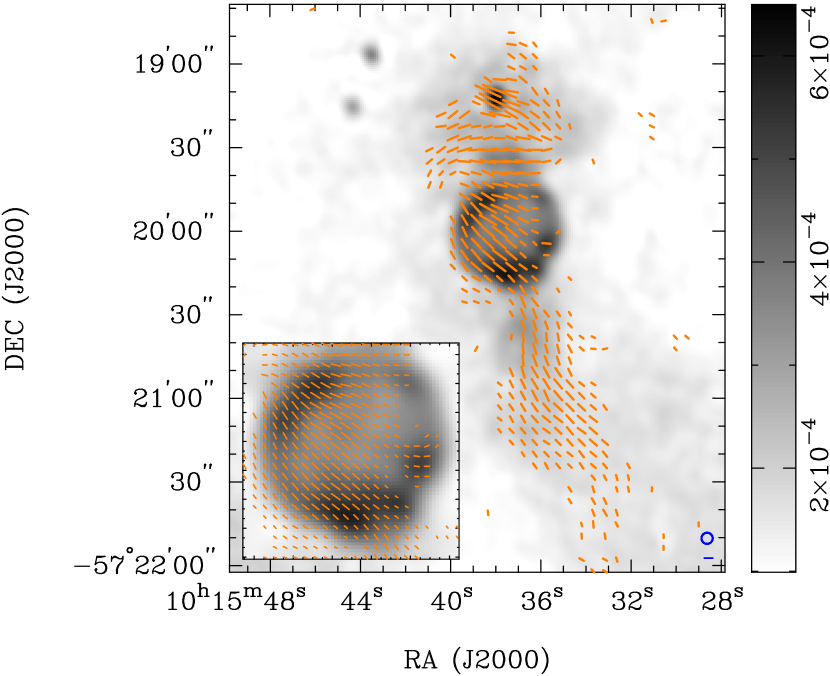
Figure 8.— The same 6 cm intensity map of J1015 and G283.1$-$0.59 as in Figure 3, overlaid with polarization $B$-vectors that indicate the intrinsic magnetic field orientation. The vector lengths are proportional to the polarized intensity at 6 cm, with the scale bar in the lower right representing of 0.1 mJy beam^-1. Vectors with uncertainties $>10\arcdeg$ in PA are clipped. The beam size is shown in the lower right. The inset is the same map zoomed in at the bubble.

The RM map was then used to correct for the Faraday rotation of the polarization vectors. The resulting map is shown in Figure 8, indicating the intrinsic orientation of the nebular magnetic field. The field appears to wrap around the head in the north and runs orthogonal to the overall nebular elongation in the interior of the head. Note that the field orientation is somewhat different at the position of J1015 than in its surroundings, which could be due to contamination by the pulsar emission. Inside the bubble, the $B$-field changes direction for $\sim$45° and runs northeast–southwest, i.e. perpendicular to the northeast rim. Intriguingly, the field follows closely the curvature of the southeast rim. It is unclear if the west rim shows the same behavior, because the degree of polarization there is too low. Just beyond the south rim, the field turns for another $\sim$45° and becomes parallel to the nebular elongation. Further south, two similar switches of the field orientation are observed. Altogether the changes in field direction seem quasi-periodic with a scale of $\sim$30″.

Finally, we simulated a polarization observation at 16 cm using the RM and intrinsic polarization maps above. We found that, due to large RM values and long wavelength, the polarization vectors rotate rapidly across the nebula. The beam depolarization effect is therefore severe for the relatively low angular resolution 16 cm observation, resulting in a very low degree of polarization, as observed.

4. Discussion

Our new radio observations reveal a remarkable nebula, G283.1$-$0.59  surrounding J1015. Its high degree of linear polarization and power-law spectrum indicate a synchrotron nature for the emission. Fundamental questions are whether this nebula is physically associated with the pulsar and what its nature is. We argue that this is a PWN system powered by J1015 based on the following results: (1) the nebula is very close in projection to the pulsar and, given its peculiar properties, a chance coincidence seems very unlikely; (2) the head of the nebula and the pulsar have comparable RM values, and the intrinsic $B$-field shows a continuous pattern across the nebula; (3) the nebular morphology is broadly similar to that of other PWNe, namely with a head that can be interpreted as a bow shock, and a circular body like the one in the Guitar Nebula (Cordes et al., 1993); and (4) the large polarization fraction and a flat spectrum are both common characteristics of radio PWNe (see Gaensler & Slane, 2006).

We should note that another possible (although less likely) interpretation of the circular structure is a supernova remnant (SNR) with fresh electrons provided by J1015. However, as we will show below, this implies an evolved and highly sub-energetic SNR, and the “tail” of the nebula as part of the remnant, which is not commonly observed. In the following discussion, we will extract the physical parameters of the nebula according to these models.

4.1. The “Head” of the Nebula as a Pulsar Bow Shock

The shape of the head is well fit by the analytic model of a bow shock with an angular separation $\theta_{0}=20\arcsec$ between the pulsar and the apex (see Figure 3). For an inclined system, we show in Appendix A that the projected shape can also be described by the same model, but the true standoff distance is always smaller than $\theta_{0}$, e.g., with inclination angles $i=60\arcdeg$, $45\arcdeg$, and $20\arcdeg$ between the bow-shock axis and the line of sight (LOS), the true standoff distance is smaller than the projected value by about 10%, 20%, and 50%, respectively (see Figure 11 in Appendix A). In our case, this implies a standoff distance $r_{0}\lesssim\theta_{0}d\approx 0.5\,$pc at the pulsar distance of $d=5$ kpc. While the exact equality holds only for a side view of the bow shock (i.e. $i=90\arcdeg$), this should be a good estimate except when its axis is very close to the LOS.

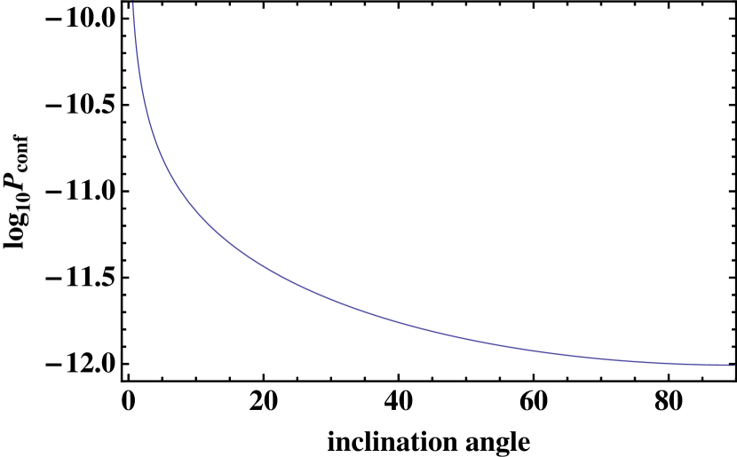
Figure 9.— Bow shock confinement pressure as a function of inclination angle.

We can then estimate the confinement pressure of the pulsar wind to be

$$P_{\rm conf}=\frac{\dot{E}}{4\pi cr_{0}^{2}}\gtrsim 10^{-12}\,\mathrm{dyn\,cm}^{-2}$$ (1)

based on the pulsar spin-down luminosity $\dot{E}=8.3\times 10^{35}$ erg s^-1. Its dependence on $i$ is plotted in Figure 9. For $i\sim 90\arcdeg$, $P_{\rm conf}$ is comparable to the typical ISM pressure in the Galactic plane (Ferrière, 2001), suggesting that the ram pressure is relatively unimportant and hence the pulsar is moving at a low Mach number. Only if the pulsar moves toward or away from us (i.e. small values of $i$), could the confinement pressure be sensibly higher. Indeed, the head shows a very diffuse morphology without a sharp boundary, which could indicate a weak confinement and support the low Mach number scenario.

4.2. Magnetic Field of G283.1$-$0.59

Since G283.1$-$0.59 is not detected in other wavebands, we estimate the average magnetic field strength based on the radio luminosity. By minimizing the total energy of the particles and the field, we obtained the so-called equipartition field

$$B_{\rm eq}=(6\pi c_{12}L/V)^{2/7},$$ (2)

where $L$ is the synchrotron luminosity, $V$ is the emission volume, and $c_{12}$ is a constant depending on the spectral index (Pacholczyk, 1970). We adopted the standard frequency range of $10^{7}$–$10^{13}$ Hz and considered only leptons in the wind with a filling factor of order unity. Taking the bubble as a sphere and the head as a cone in 3D, we estimated $B_{\rm eq}\sim 70\,\mu$G and $\lesssim 60\,\mu$G, respectively. These values are similar to those found in other systems (e.g., Ng et al., 2010, 2012). Their associated total energies are both about $E_{\rm eq}\sim 10^{46}\,$erg. Note that any deviations from equipartition would imply higher total energies.

If these structures are efficiently powered by the spin-down of J1015, the time scale to fill them could be very short $\sim(E_{\rm eq}^{\rm bubble}+E_{\rm eq}^{\rm head})/\dot{E}\sim 700$ yr. The synchrotron cooling time, on the other hand, is much longer. Even for particles emitting at the highest observed frequency of $\nu\approx 10$ GHz (Figure 5), the cooling time

$$\tau_{\rm syn}=45\left(\frac{B}{\rm 10\,\mu G}\right)^{-3/2}\left(\frac{\nu}{\rm 10\,GHz}\right)^{-1/2}\,\mbox{Myr}$$ (3)

exceeds the pulsar’s characteristic age of $\tau_{c}=39$ kyr by three orders of magnitude. It is therefore justified to neglect synchrotron loss and the radio morphology of G283.1$-$0.59 traces the motion of J1015, i.e. moving north at a PA of $\sim$5°. We can then infer another time scale from the offset $r_{\rm offset}$ between the pulsar’s current location and the bubble center (assuming the bubble is at rest)

$$\tau_{\rm offs}=\frac{r_{\rm offset}}{v_{\rm psr,\perp}}\simeq 1.2\times 10^{4}\left(\frac{v_{\rm psr,\perp}}{\rm 100\,km\,s^{-1}}\right)^{-1}\,\mbox{yr}.$$ (4)

The pulsar projected velocity $v_{\rm psr,\perp}$ has not yet been measured, and the only inference we can make about it from all the clues is a low Mach number. If this is the case, $\tau_{\rm offset}$ could easily be of the order of $\tau_{c}$. Incidentally, this coincidence seems to suggest that the bubble started forming when the pulsar was much younger than now, which opens the way to an alternative scenario, namely that the bubble coincides with the position of an associated SNR. This scenario will be considered in Section 4.5 below.

Interestingly, the projected spin axis of J1015 has a PA of 62° (or 152° if the pulsar emission is in the orthogonal mode) (Johnston & Weisberg, 2006). Either case shows a significant misalignment with the pulsar motion direction (PA $\sim$5°) inferred from the nebular elongation. While this may seem uncommon among young isolated neutron stars (see e.g., Johnston et al., 2005; Noutsos et al., 2012), simulations of neutrino kicks indicate that a large misalignment angle is more likely to be found in low-velocity pulsars (Ng & Romani, 2007). This provides an indirect support for the low Mach number we argued above.

Our radio polarization measurement revealed a highly ordered magnetic field structure in G283.1$-$0.59. As shown in Figure 8, the intrinsic $B$-field wraps around the northern edge of the nebula. This is the first time such a structure has been observed in bow shocks. It could indicate that the magnetic field follows the shocked pulsar wind to sweep back due to the pulsar motion. For bow shocks with high Mach number, the opening angle of the head is generally much smaller. This structure is therefore more difficult to be resolved by the observations. Inside the head, the $B$-field exhibits an azimuthal geometry perpendicular to the nebular elongation, implying a helical field trailing the pulsar. Unlike the more common case of a parallel configuration, e.g., the Mouse and the Frying Pan (Yusef-Zadeh & Gaensler, 2005; Ng et al., 2012), a helical field has only previously been found in one bow shock PWN, namely, G319.9$-$0.7 (Ng et al., 2010). The latter is believed to be moving faster than J1015, at a few hundred  km s^-1 (Klingler et al., 2016). While an azimuthal field could be generated by a supersonically moving pulsar with aligned spin and velocity (Romanova et al., 2005), this may not apply to J1015 as we have evidence for a large misalignment angle. Our results imply that the $B$-field configuration in bow shocks may depend more on the flow condition and other physical parameters rather than the Mach number or the pulsar spin–velocity alignment. Unfortunately the flow speed in G283.1$-$0.59 is not easy to determine since no synchrotron loss is observed in the radio band. It is essential to expand the bow shock sample for further investigation.

The magnetic field changes direction quasi-periodically south of the bubble and along the tail. Similar behavior has been found in two other bow shock PWNe: the Mouse and G319.9$-$0.7 (Yusef-Zadeh & Bally, 1987; Ng et al., 2010). Intriguingly, the latter also exhibits a bulge morphology and the intrinsic field orientation switches from azimuthal to parallel configuration near the bulge, as in our case. The switches could be related to instabilities in the flow, which may have created the bubble and the bulge, although the exact mechanism is still unclear. We note that instabilities generally lead to a turbulent environment and it remains to be explained how the high observed degree of polarization is preserved. One possible solution is a large characteristic scale for the turbulence, similar to what was found in the Snail (Ma et al., 2016). Further studies with magnetohydrodynamic simulations are needed to understand the cause and scale of the instabilities. Finally, turbulence in the interstellar environment could also cause kinks in the tail and change the $B$-field direction (e.g., the Frying Pan; Ng et al., 2012), but it cannot produce the bubble structure.

4.3. The Bubble as an Expanding Shell

The equipartition $B$-field strengths in Section 4.2 imply total (magnetic + particle) pressures of at least $\sim 200\times 10^{-12}$ dyn cm^-2 and $\sim 300\times 10^{-12}$ dyn cm^-2 inside the head and the bubble respectively, both much larger than the typical ISM pressure of $\sim 10^{-12}$ dyn cm^-2. While in the head this could still be consistent with a low pulsar Mach number (around 8–10), the overpressure issue in the bubble is very significant (and could be even more severe in the case of deviations from equipartition). Indeed as Figure 8 shows, the $B$-field generally follows the curvature of the bubble rim in the southeast, indicating that it could be swept up by an expanding shell (see e.g., Kothes & Brown, 2009; Bandiera & Petruk, 2016). This would compress the field at the rim and result in higher emissivity than in the interior. Together with projection effects, these lead to the limb-brightened structure of the bubble. The surface brightness of the bubble peaks in the northeast and the southwest where the rim is perpendicular to the $B$-field. Similar behavior is typically observed in young SNRs (e.g., Dubner & Giacani, 2015) and the enhanced radio emission is interpreted as evidence of efficient particle acceleration when the magnetic field is quasi-parallel to the shock direction. However this does not work in our case, since it would induce a strongly turbulent field and re-acceleration of the pulsar wind, resulting in a very low degree of polarization and a steep radio spectrum incompatible with the observations.

We instead propose another scenario: that the bubble acts as a “magnetic bottle” and traps the relativistic particles. Due to conservation of magnetic flux, the expansion of the bubble creates a gradient in the magnetic field along the northeast–southwest direction. A particle moving toward the equatorial zone would then show a decrease in the pitch angle and an increase in the longitudinal velocity. The opposite occurs when it moves away from the equatorial zone. Particles entering from one side of the bubble should, in principle, be able to exit from the other side. However, the presence of scattering broadens the pitch angle distribution. Some particles could therefore have pitch angles over 90° before exiting the bubble, i.e. they would be mirrored back. The lower polarization fraction observed near the rim of the bubble could suggest a mild level of turbulence, providing some degree of scattering and helping the confinement.

Note that in order for the electrons to bounce back and forth, the mean free path parallel to the direction of the ordered magnetic field ($\lambda_{\parallel}$) should be no smaller than the bubble radius ($R_{\rm bubble}$). The former is proportional to the gyroradius ($r_{g}$) with

$$\lambda_{\parallel}=\eta r_{g}\sim 3.5\times 10^{12}\left(\frac{\nu}{\rm 5\,GHz}\right)\left(\frac{B}{\rm 10\,\mu G}\right)^{-3/2}\eta\,\mbox{cm},$$ (5)

where $\eta=(\delta B/B)_{\rm res}^{-2}$ is related to the perturbation of the magnetic field resonant with the radio emitting particles (Reynolds, 1998). The condition $\lambda_{\parallel}\gtrsim R_{\rm bubble}$ implies

$$\left(\frac{\delta B}{B}\right)_{\rm res}\lesssim 1.5\times 10^{-3}\left(\frac{\nu}{\rm 5\,GHz}\right)^{1/4}\left(\frac{B}{\rm 10\,\mu G}\right)^{-3/4}.$$ (6)

This in not unreasonable, considering that in a (Kolmogorov-like) turbulent cascade $(\delta B/B)_{\rm res}$ decreases at smaller scales. This suggests $\eta\gg 1$, hence diffusion perpendicular to the magnetic field has a small mean free path ($r_{\perp}\approx r_{g}/\eta$) and is very inefficient. As a result, electrons can be considered as frozen into their original flux tubes.

The synchrotron emission of the bubble primarily comes from particles injected by the pulsar wind with the magnetic field mostly swept-up from the surroundings. The observed limb brightening can be explained by: (1) particles near the center emit mostly in directions off the observer LOS, due to the geometry of the magnetic bottle, (2) they also emit less effectively due to generally lower pitch angles, and (3) the higher longitudinal velocities of the particles in the equatorial zone imply a lower number density and hence a lower emissivity compared with the polar regions.

From a dynamical point of view, these trapped particles would be responsible for most of the pressure inflating the bubble. It can be shown that, for a Kolmogorov-like power spectrum of magnetic fluctuations, the parallel mean free path of particles is proportional to their Lorentz factor as $\gamma^{-2/3}$; i.e. higher-energy electrons (than the radio-emitting ones), which carry most of the energy, reach an isotropic velocity distribution more efficiently inside the bubble, likely providing the required pressure. The expansion of the bubble can only be balanced by the inertia of the ambient medium. A simple dimensional argument suggests that in this case the total energy of the bubble must be comparable with $\sim$$\rho_{0}R_{\rm bubble}^{5}/t_{\rm exp}^{2}$, where $\rho_{0}$ is the ambient density and $t_{\rm exp}$ is the bubble expansion time. We can then use the equipartition $B$-field result in Equation (2) to estimate the ambient density

$$n_{0}\sim 10^{3}\left(\frac{t_{\rm exp}}{\tau_{c}}\right)^{2}\,\mbox{cm}^{-3}.$$ (7)

If $t_{\rm exp}\approx\tau_{\rm offs}$ is of the order of $\tau_{c}$, the environment must be very dense to keep the bubble confined. Otherwise a very young bubble would imply a high pulsar velocity to explain the observed offset, and this is in contrast to what was previously deduced on the basis of the properties of the nebular head. It is therefore more likely that the bubble is expanding into a dense medium.

Driven by the above considerations, we have then checked whether there is evidence of a dense surrounding medium. In the optical catalogs (Feitzinger & Stuewe, 1984; Dutra & Bica, 2002), we found two dark clouds, FeSt2-78 and FeSt2-79, coinciding with G283.1$-$0.59 (see Figure 1). This LOS is near the Sagittarius–Carina arm tangent ($l=282\arcdeg$), which has a distance of $\sim$4 kpc (Graham, 1970), broadly consistent with that of J1015. Hence, the clouds are possibly in the pulsar vicinity. Based on the difference between the central and background reddening of the clouds (Dutra & Bica, 2002), we estimate their optical extinction and hydrogen column densities using empirical relations (Fitzpatrick, 2004; Güver & Özel, 2009). The latter give densities of $n_{0}\sim 450$ cm^-3 and $\sim$680 cm^-3 for FeSt2-78 and FeSt2-79, respectively, assuming spherical clouds with 6′ angular diameter (Dutra & Bica, 2002) at the pulsar distance of 5 kpc. Following the same procedure, we estimate the density of all dark clouds in the above catalogs with $\Delta l=\pm 20\arcdeg$ from J1015 and $|b|<1\arcdeg$. There are only five objects with density higher than 450 cm^-3 and their total area in the sky suggests a chance coincidence of 0.1% to have a dense cloud overlapping with G283.1$-$0.59. We argue that the PWN is in a dense environment with $n_{0}$ of a few hundred cm^-3, as inferred from our analysis.

4.4. Origin of the Bubble

We now turn to the origin of the bubble. The flat radio spectrum of the bubble indicates that it is part of the PWN structure. There are several possible scenarios in which an extended nebula could be formed at a distance from the pulsar: (1) a relic nebula crushed by the supernova reverse shock, (2) injection of pulsar wind into a pre-existing cavity such as a stellar wind bubble, (3) sudden expansion of the flow due to mass loading (Morlino et al., 2015), and (4) an expanding bubble driven by flow instabilities (e.g., van Kerkwijk & Ingle, 2008). The first two scenarios would be viable only if the associated shell-type SNR no longer emits in radio and the ordered longitudinal magnetic field between the pulsar and the bubble could be explained. The $B$-field and the limb brightness structure of the bubble do not seem to match what is seen in a relic PWN, such as G327.1$-$1.1 (Temim et al., 2015; Ma et al., 2016). Also in this case the “tail” of the nebula would be a blowout of the SNR and happen to be in the opposite direction to the pulsar by chance. Finally, mass loading generally does not produce a circular structure.

To explore the instabilities scenario, we follow van Kerkwijk & Ingle (2008) to assume that the post-shock flow became unstable downstream, injecting a fraction $f_{\dot{E}}$ of the spin-down energy into the bubble. The total injected energy into the bubble is

$$E_{0}\simeq f_{\dot{E}}\dot{E}t_{\rm exp}\simeq 10^{48}f_{\dot{E}}\left(\frac{t_{\rm exp}}{\tau_{c}}\right)\,\mbox{erg}.$$ (8)

If the flow instability occurred in a short timescale and the bulk of the energy was released a long time ago, the evolution should be similar to that of an SNR, in spite of the different energy scale. We employed an analytic model developed by Bandiera & Petruk (2004) to follow both the adiabatic and radiative phases of the SNR evolution (Truelove & McKee, 1999). The bubble radius in the adiabatic phase can be described by the standard Sedov–Taylor solution,

$$R_{\rm bubble}(t_{\rm exp})=1.152\left(\frac{\mbox{$\dot{E}$}}{\rho_{0}}\right)^{1/5}t_{\rm exp}^{2/5}.$$ (9)

The transition to the radiative phase occurs at time and radius of

$$t_{\rm tran}\simeq 2.9\times 10^{4}\left(\frac{E_{0}}{\rm 10^{51}\,erg}\right)^{4/17}\left(\frac{n_{0}}{\rm 1\,cm^{-3}}\right)^{-9/17}\mbox{yr}\quad\mbox{and}$$ (10)

$$R_{\rm tran}\simeq 19.1\left(\frac{E_{0}}{\rm 10^{51}\,erg}\right)^{5/17}\left(\frac{n_{0}}{\rm 1\,cm^{-3}}\right)^{-7/17}\mbox{pc},$$ (11)

and the radiative phase can be described by the inverse evolutionary relation

$$t^{\prime}(R^{\prime})=\frac{2}{35}\sqrt{R^{\prime}-1}\left(5R^{\prime 3}+6R^{\prime 2}+8R^{\prime}+16\right)-0.248,$$ (12)

where $t^{\prime}=t/(1.14\,t_{\rm tran})$ and $R^{\prime}=R/(0.85\,R_{\rm tran})$. Figure 10 (left) shows a diagnostic plot of the ambient density and age that gives the observed $R_{\rm bubble}=0.5$ pc. For $n_{0}\sim 500$ cm^-3 and $t_{\rm exp}\sim 4\times 10^{4}$ yr, a total energy of $\sim 10^{47}$ erg is sufficient to give rise to the bubble, i.e. $f_{\dot{E}}$ of the order of 10%. We also illustrate in the plot estimates with only the Sedov–Taylor solution: in this case the constraints on $n_{0}$ are overestimated by an order of magnitude for a given age. This highlights the importance of correctly accounting for the transition to the radiative phase.

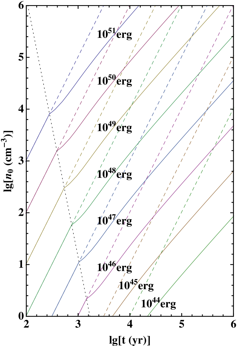
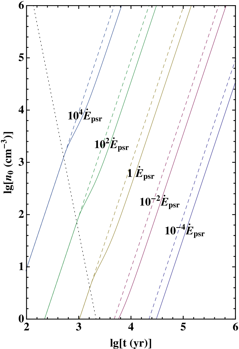
Figure 10.— Bubble expansion time ($t$) and ambient density ($n_{0}$) that give the observed bubble radius of 0.5 pc. Left: the case of sudden initial energy release as in an SNR, according to the evolution model by Bandiera & Petruk (2004). The solid color lines represent different total energies. The transition from the Sedov phase to the radiative phase, which is indicated by the black dotted line, leads to a power-law evolution with a different slope. The dashed lines show the extrapolation of the adiabatic evolution. It is apparent that using the adiabatic extrapolation largely overestimates $n_{0}$ for a given $t$. Right: the same for a bubble with constant energy injection rates. The evolution curves transit from adiabatic to radiative regimes smoothly, and eventually approach a trend parallel to the original one.

If instead the bubble has been constantly powered by J1015 with constant $\dot{E}$ until the present time, Dokuchaev (2002) developed the adiabatic solution

$$R_{\rm bubble}(t_{\rm exp})=0.929\left(\frac{\mbox{$\dot{E}$}}{\rho_{0}}\right)^{1/5}t_{\rm exp}^{3/5}.$$ (13)

We show in Appendix B that this solution also applies to the asymptotic radiative phase with a scaling factor of 0.821. The result is plotted in Figure 10 (right). For $n_{0}\sim 500$ cm^-3 and $t_{\rm exp}\sim 4\times 10^{4}$ yr, $f_{\dot{E}}\sim 1\%$ is sufficient.

4.5. Where is the SNR?

With a characteristic age of only 39 kyr, the true age of J1015 should be of the same order or smaller, such that the parent SNR may still be visible. As discussed, the elongation of G283.1$-$0.59 indicates the pulsar’s direction of motion. In this region of the sky there are only SNR G284.3$-$1.8 (Williams et al., 2015) and a candidate SNR G282.8$-$1.2 (Misanovic et al., 2002). However, neither of them aligns with the nebula. There is also no known massive star cluster in the general direction. As we argued in Section 4.1, the pulsar could be traveling at a low velocity, hence the supernova site should not be too far from the pulsar’s current location, possibly within the same dense clouds we found in the catalog. If this is the case, the SNR could have already evolved to a late stage and become unobservable.

Another possibility to investigate is whether the radio bubble is indeed the parent SNR of J1015. If the pulsar were born at the bubble center, the offset to its current location would imply a traverse velocity significantly larger than the SNR expansion rate, with $v_{\rm psr,\perp}/v_{\rm snr}=r_{\rm offset}/R_{\rm bubble}=2.5$. A more serious issue with this picture is that the high ambient density observed is not sufficient by itself to account for the small physical size of the bubble if it is an SNR; an exceptionally sub-energetic supernova explosion is also required. As we discussed in Section 4.3 and showed in Figure 10, the observed bubble size implies a total energy of $\sim 10^{47}$ erg. This is much lower than the typical supernova energy of $10^{51}$ erg.

In this scenario, the sub-energetic SNR has evolved well beyond the Sedov phase, thus the particle acceleration efficiency should have decreased considerably (Bandiera & Petruk, 2010). Although the magnetic structure of G283.1$-$0.59 belongs to the relic SNR, it is only detectable in radio because leptons are provided by the pulsar to power the synchrotron emission. This is also what the flat radio spectrum seems to suggest. This situation could be similar to the case of SNR G5.4$-$1.2, which shows a pulsar and associated PWN outside (while not far from) the SNR boundary. The radio spectral index of the SNR limb is flatter when close to the pulsar position (Frail et al., 1994), a fact that could be attributed to the radio emission from leptons with a hard energy distribution leaking from the PWN. In short, the interpretation of the bubble as an SNR would be tenable under various aspects, except for the requirement of $E_{0}$ about $10^{4}$ times smaller than the average, making it rather unlikely.

5. Conclusion

We presented radio observations of the field of PSR J1015$-$5719 at 36, 16, 6, and 3 cm taken with MOST and ATCA. The radio images revealed a nebula, G283.1$-$0.59, consisting of a diffuse head, a circular bubble, and a collimated tail. Based on its positional coincidence with the pulsar, its flat spectrum, and high degree of linear polarization, we suggest that the source is a newly discovered PWN system with the head as a bow shock moving at a low Mach number and the bubble as a shell expanding in a dense medium. We also considered an alternative scenario with the bubble as the parent SNR of the pulsar. However, this requires a supernova explosion energy much smaller than the canonical value, which does not seem plausible.

G283.1$-$0.59 presents a rare example of a slow-moving bow-shock PWN, in which the pulsar spin axis misaligns with the proper motion direction. On the other hand, it shows similar $B$-field geometry and expanding bubble feature as in other higher Mach number systems. This implies that the bow shock properties could depend more on other factors, such as the flow condition, instead of the pulsar velocity.

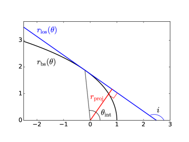
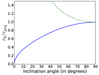
Figure 11.— Left: illustration of the projected bow-shock standoff distance $r_{\mathrm{proj}}$. The black line is the bow-shock model given by Wilkin (1996) and the blue line shows the line of sight with an inclination angle $i$. The axes are in units of $r_{0}$, the true standoff distance. Right: the ratio between $r_{0}$ and $r_{\mathrm{proj}}$ as a function of inclination angle (blue solid line). Note that the $r_{\mathrm{proj}}$ is always larger than $r_{0}$ and the result is invariant under a transform of $i$ to $180\arcdeg-i$. A simple $1/\sin i$ relation is plotted by the green dashed line for comparison.

Appendix A Projected Standoff Distance and Shape of an Inclined Bow Shock

We start from the analytic formula derived by Wilkin (1996), which describes a bow shock shape in polar coordinates:

$$r_{\mathrm{bs}}(\theta)=r_{0}|\csc\theta|\sqrt{3(1-\theta\cot\theta)},$$ (A14)

where $r_{\mathrm{bs}}$ is the radial distance from the origin (i.e. the position of the star) and $-\pi<\theta<\pi$ is the polar angle from the direction of the standoff point, expressed in radians. The shape described by the above equation is universal, while the relative strength of the stellar wind and the ambient ram pressure determine only the spatial scale of the bow shock, namely $r_{0}$. Of course, the exact shape described by Equation (A14) could actually be observed only when the viewing angle is orthogonal to the stellar velocity direction (i.e. inclination angle $i=90^{\circ}$). We investigate here how the projected standoff distance, $r_{\mathrm{proj}}$, as well as the projected shape of an inclined bow shock, depend on the inclination angle.

We first limit our analysis to the symmetry plane identified by the direction of the standoff point and the LOS and passing through the origin. The LOS with slope $b=\tan i$ ($i$ is defined modulo $\pi$ radians) and a generic projected displacement $a_{\mathrm{proj}}$ from the origin can be described by

$$r_{\mathrm{los}}(\theta)=\frac{a_{\mathrm{proj}}\sqrt{1+b^{2}}}{b\cos\theta-\sin\theta}$$ (A15)

in polar coordinates. Note that $r_{\mathrm{los}}$ changes sign if $\theta$ shifts by $\pi$ radians. However, in polar coordinates it identifies the same point. For a given value of $b$, if the bow shock and the LOS intersect at $r_{\mathrm{bs}}(\theta_{\rm int})=r_{\mathrm{los}}(\theta_{\rm int})$, the projected distance from the origin is then

$$a_{\mathrm{proj}}(\theta_{\rm int})=r_{0}\,{\rm sgn}(\theta_{\rm int})(b\cot\theta_{\rm int}-1)\sqrt{\frac{3(1-\theta_{\rm int}\cot\theta_{\rm int})}{1+b^{2}}}.$$ (A16)

Consider a family of LOS with the same slope $b$ but intersecting the bow shock at different $\theta_{\rm int}$; the one tangent to the bow shock should have largest $a_{\mathrm{proj}}$ and hence $a_{\mathrm{proj}}=r_{\mathrm{proj}}$ in this case (see Figure 11 left). This can be done analytically by putting ${\rm d}a_{\mathrm{proj}}(\theta_{\rm int})/{\rm d}\theta_{\rm int}=0$. The resulting formula is rather cumbersome, but it can be simplified to

$$(\sin\theta_{\rm int})(\theta_{\rm int}-\sin\theta_{\rm int}\cos\theta_{\rm int})-b\left[3\cos\theta_{\rm int}\right.$$

$$\times\left.(\theta_{\rm int}-\sin\theta_{\rm int}\cos\theta_{\rm int})-2\sin^{3}\theta_{\rm int}\right]=0.$$ (A17)

Solving this equation for $\theta_{\rm int}$ is very complex, but the solution for $b$ is trivial:

$$b( \theta_{\rm int} )=\tan[i(\theta_{\rm int})]$$ (A18)

$$= \frac{\sin\theta_{\rm int}(\theta_{\rm int}-\sin\theta_{\rm int}\cos\theta_{\rm int})}{3\cos\theta_{\rm int}(\theta_{\rm int}-\sin\theta_{\rm int}\cos\theta_{\rm int})-2\sin^{3}\theta_{\rm int}}$$

(a sign change in $\theta_{\rm int}$ implies a sign change in $b$ and hence in $i$). Hence, for any values of intersection $\theta_{\rm int}$, we can easily derive the related inclination angle: for that angle, and only for that, Equation (A16) actually gives $r_{\mathrm{proj}}$. Figure 11 (right) shows the resulting $r_{\mathrm{proj}}$ as a function of $i$, obtained from a parametric plot with $\theta_{\rm int}$ as the variable and the $x$ and $y$ values from Equations (A18) and (A16). The result indicates that $r_{\mathrm{proj}}$ is always larger than the true standoff distance $r_{0}$ for any $i$ (except for $i=\pm 90\arcdeg$, when it is equal to $r_{0}$) and it is different from the simple $\sin i$ dependence. The latter, which was used by some authors in previous studies to correct for the orientation, is therefore not even qualitatively correct.

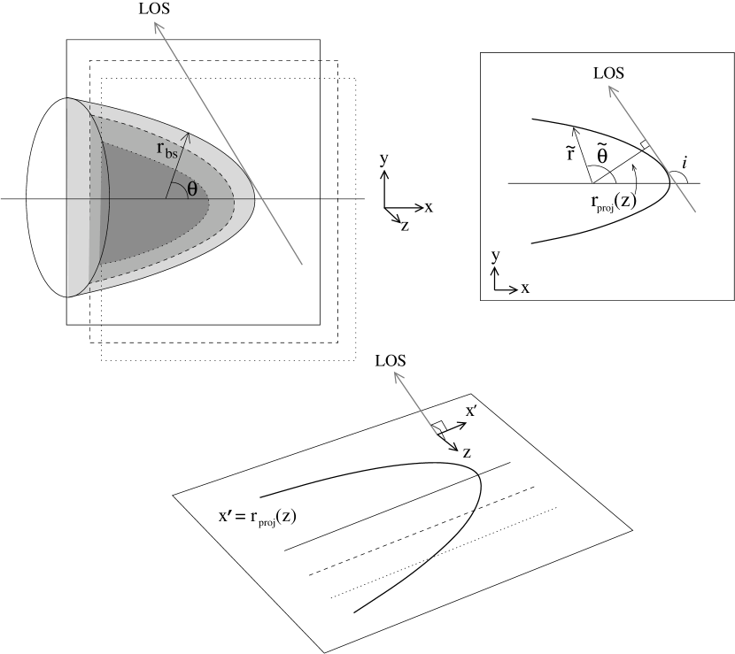
Figure 12.— Illustration of a bow shock projected onto the plane of the sky and sliced in the $z$ direction. This also indicates the choice of coordinate system and symbols used in the calculation.

A similar approach can also be used to derive the position of the projected limb along any LOS, and ultimately, to derive the shape of the bow shock projected at a generic inclination angle. We define a coordinate system such that: $x$ is directed along the bow shock axis, toward its apex; $y$ is the orthogonal axis lying on the plane defined by $\hat{x}$ and the LOS; and $z$ is orthogonal to the previous two. Define $x^{\prime}$ as the $x$-axis projected onto the plane of the sky, then the shape of the projected bow shock is given by a function $x^{\prime}=r_{\mathrm{proj}}(z)$, where the $z$ coordinate of a point gives the displacement from the projected axis (see Figure 12). We first slice the bow shock along the $z$ direction. For a given $z$ value, the slice of the bow shock in the $x$–$y$ plane can be described by a function $\tilde{r}(\tilde{\theta})$, where $\tilde{\theta}$ is the 2D polar angle. $\tilde{r}$ is related to $r_{\mathrm{bs}}$ and $z$ by

$$r_{\mathrm{bs}}^{2}=\tilde{r}^{2}+z^{2}\quad\mbox{and}$$ (A19)

$$r_{\mathrm{bs}}\cos\theta=\tilde{r}\cos\tilde{\theta}.$$ (A20)

In Equation (A20), the condition to have a solution for $\tilde{\theta}$ is

$$z^{2}\leqslant r_{\mathrm{bs}}^{2}\sin^{2}\theta=3(1-\theta\cot\theta).$$ (A21)

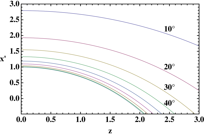
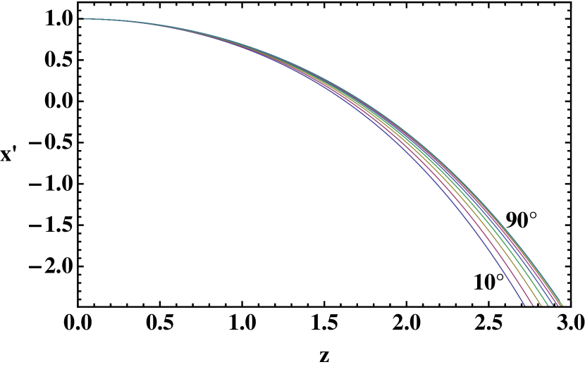
Figure 13.— Left: projected shapes of a bow-shock model by Wilkin (1996) with different inclination angles. Right: the same plot scaled by $1/r_{\mathrm{proj}}(\theta_{\rm int},0)$ to match the projected standoff distance. In both plots, the axes are in units of $r_{0}$ and the lines represent different inclination angles of from 10° to 90°. (See Figure 11 for the definition of the inclination angle, $r_{0}$, and $r_{\mathrm{proj}}$.)

In an analogous way as we did with Equation (A15), we define

$$x_{\mathrm{los}}(\tilde{\theta})=\frac{a_{\mathrm{proj}}\sqrt{1+b^{2}}}{b\cos\tilde{\theta}-\sin\tilde{\theta}}$$ (A22)

and take its intersection with $\tilde{r}$ at $\tilde{\theta}_{\rm int}$, i.e. $\tilde{r}(\tilde{\theta}_{\rm int})=x_{\mathrm{los}}(\tilde{\theta}_{\rm int})$. After some simplification, we obtain the projected elongation (the equivalent in 3D of Equation (A16))

$$a_{\mathrm{proj}}(\theta_{\rm int},z)=r_{0}\left[b\cot\theta_{\rm int}\sqrt{3(1-\theta_{\rm int}\cot\theta_{\rm int})}\right.$$

$$-\left.\sqrt{3(1-\theta_{\rm int}\cot\theta_{\rm int})-z^{2}/r_{0}^{2}}\right]\bigg{/}\sqrt{1+b^{2}}.$$ (A23)

Following the same procedure as before, we take the derivative and finally derive

$$b( \theta_{\rm int} ,z)=\tan[i(\theta_{\rm int},z)]=\sqrt{\frac{3(1-\theta_{\rm int}\cot\theta_{\rm int})}{3(1-\theta_{\rm int}\cot\theta_{\rm int})-z^{2}/r_{0}^{2}}}$$ (A24)

$$\times \frac{\sin\theta_{\rm int}(\theta_{\rm int}-\sin\theta_{\rm int}\cos\theta_{\rm int})}{3\cos\theta_{\rm int}(\theta_{\rm int}-\sin\theta_{\rm int}\cos\theta_{\rm int})-2\sin^{3}\theta_{\rm int}}.$$

As a check, for $z=0$, the factor within the square root reduces to unity, and hence Equation A18 is recovered.

As illustrated in Figure 12, for a given offset $z$, figures equivalent to Figure 11 (right) can now be easily obtained as parametric plots of the variable $\theta_{\rm int}$ (where $\theta_{\rm int}$ satisfies the condition in Equation (A21)) using Equations (A24) and (A23). This gives $r_{\mathrm{proj}}(\theta_{\rm int},z)$, the coordinate of the projected limb along the $x^{\prime}$ axis. By performing this calculation for all $z$ and $\theta_{\rm int}$ values, $r_{\mathrm{proj}}$ for all values of $i$ can be obtained. On the other hand if $i$ is given, we need to solve Equation (A24) to get $\theta_{\rm int}(z,i)$ (this is the only part of the procedure that still needs to be done numerically). The projected profiles of different inclination angles are shown in Figure 13 (left). As $i$ decreases from 90°, $r_{\mathrm{proj}}$ increases but the overall shape remains similar. In real life, $r_{\mathrm{proj}}$ is often the only observable while $i$ or $r_{0}$ are unknown; we therefore scale the plot by $1/r_{\mathrm{proj}}(\theta_{\rm int},0)$ for comparison and the result is shown in Figure 13 (right). Obviously, the change in the projected shape is minimal and thus very difficult to distinguish between them from observations. Hence, we conclude that the same analytic solution is a sufficiently good approximation also for inclined cases with $i$ different from 90°.

Appendix B Expansion of a Bubble with Continuous Injection in a Uniform Medium

We present here a thin-shell model of an expanding bubble in a homogeneous ambient medium, in the case of a continuous energy release at a constant rate $\dot{E}$. The approach is similar to that presented by Bandiera & Petruk (2004), for an initial energy of the bubble. We will also model the transition from adiabatic to radiative phases.

The basic assumptions are that matter is confined to a thin, spherically symmetric shell at the boundary of the bubble, which contains all the kinetic energy of the system, while all the thermal energy is contained in the homogeneous interior of the bubble. The conservation of mass and momentum in the shell are described by the equations

$$\frac{{\rm d}M}{{\rm d}t}=4\pi\rho_{0}R^{2}\dot{R}\quad\mbox{and}$$ (B1)

$$\frac{{\rm d}(M\dot{R})}{{\rm d}t}=4\pi PR^{2},$$ (B2)

where $M$ and $R$ are the mass and the radius of the shell, respectively, $P$ is the pressure, and $\rho_{0}$ is the ambient density. The above equations can be rearranged into

$$M=\frac{4\pi}{3}\rho_{0}R^{3}\quad\mbox{and}$$ (B3)

$$\ddot{R}+\frac{3\dot{R}^{2}}{R}=\frac{3}{\rho_{0}}\frac{P}{R}.$$ (B4)

Conservation of energy (total energy of the bubble in the adiabatic phase) leads to the following equation for the pressure (we adopt an adiabatic index $\gamma=5/3$)

$$\frac{{\rm d}P}{{\rm d}t}=\frac{\dot{E}}{2\pi R^{3}}-5P\frac{\dot{R}}{R}+\frac{\rho_{0}\dot{R}^{3}}{R}.$$ (B5)

Instead, in the so-called radiative phase, only the internal energy of the bubble is conserved, leading to

$$\frac{{\rm d}P}{{\rm d}t}=\frac{\dot{E}}{2\pi R^{3}}-5P\frac{\dot{R}}{R}~{}.$$ (B6)

In Bandiera & Petruk (2004) the energy was injected just at the initial time by the supernova, so that $\dot{E}$ is zero, while here we consider the case of vanishing initial energy but with a constant $\dot{E}>0$, which is more suitable to describe a PWN powered by a long-lived pulsar. By introducing the quantity

$$y(R)=R^{6}\dot{R}^{2},$$ (B7)

one can transform the equations above into

$$y^{\prime\prime}(R)=\frac{3\dot{E}R^{5}}{\pi\rho_{0}\sqrt{y}}+\left(\frac{6y}{R^{2}}\right)_{\rm ad},$$ (B8)

where the term with suffix “ad” is added only when treating the adiabatic phase. One can show that $y(R)=Q^{2}R^{14/3}$ is a special solution for both the adiabatic and the radiative equations, with

$$Q_{\rm ad}=\frac{3}{5^{2/3}}\left(\frac{\dot{E}}{4\pi\rho_{0}}\right)^{1/3}\quad\mbox{and}$$ (B9)

$$Q_{\rm rad}=\frac{3\cdot 2^{1/3}}{77^{1/3}}\left(\frac{\dot{E}}{4\pi\rho_{0}}\right)^{1/3},$$ (B10)

respectively. The full transition from the adiabatic to the asymptotic radiative case requires us to solve (numerically) Equation (B8), by imposing the continuity of $y(R)$ and $y^{\prime}(R)$ at the transition. Finally, given $y(R)$, the time evolution can be computed by solving (numerically also in this case) Equation (B7) for $R(t)$. In the asymptotic cases i.e. Equations (B9) and (B10) above, the solutions are:

$$R(t)=\left(\frac{5}{3}Qt\right)^{3/5}.$$ (B11)

Figure 14.— Transition from the adiabatic phase to the radiative phase for a bubble expanding in a uniform medium with continuous energy injection. The asymptotic behavior in these cases only differs by a small constant factor of 0.821 (see Dokuchaev, 2002, and Equations (B9)–(B11)).

Therefore, it is apparent that here, apart from a small offset, both the adiabatic and the asymptotic radiative phases have the same power-law dependence on time. This is qualitatively different from the case with an energy release at the initial time, in which the adiabatic (Sedov) phase has $R(t)\propto t^{2/5}$, while the asymptotic radiative (or “pressure-driven snowplow”) phase has $R(t)\propto t^{2/7}$. This is also different from the behavior of a PWN expanding inside an SNR (e.g., Reynolds & Chevalier, 1984), since we assumed a static ambient medium. For the adiabatic regime, the radius estimated here in the thin-layer approximation is only about 10% smaller (a factor 0.895) than the true value, as computed by Dokuchaev (2002); for the radiative phase, as the layer of matter is thinner, we expect the true value of the radius to be approximated even better. Using the correct coefficient for adiabatic evolution, the asymptotic radiative solution is smaller than the extrapolation of the adiabatic one by a constant factor 0.821. Figure 14 shows the radial evolution at intermediate times.

References

- Acero et al. (2015) Acero, F., Ackermann, M., Ajello, M., et al. 2015, ApJS, 218, 23
- Bandiera & Petruk (2004) Bandiera, R., & Petruk, O. 2004, A&A, 419, 419
- Bandiera & Petruk (2010) —. 2010, A&A, 509, A34
- Bandiera & Petruk (2016) —. 2016, MNRAS, 459, 178
- Ben Bekhti et al. (2016) Ben Bekhti, N., Flöer, L., Keller, R., et al. 2016, A&A, 594, A116
- Bock et al. (1999) Bock, D. C.-J., Large, M. I., & Sadler, E. M. 1999, AJ, 117, 1578
- Briggs (1995) Briggs, D. S. 1995, BAAS, 27, 1444
- Campbell-Wilson & Hunstead (1994) Campbell-Wilson, D., & Hunstead, R. W. 1994, PASA, 11, 33
- Cordes & Lazio (2002) Cordes, J. M., & Lazio, T. J. W. 2002, astro-ph/0207156
- Cordes et al. (1993) Cordes, J. M., Romani, R. W., & Lundgren, S. C. 1993, Nature, 362, 133
- Dame et al. (2001) Dame, T. M., Hartmann, D., & Thaddeus, P. 2001, ApJ, 547, 792
- Dokuchaev (2002) Dokuchaev, V. I. 2002, A&A, 395, 1023
- Dubner & Giacani (2015) Dubner, G., & Giacani, E. 2015, A&A Rev., 23, 3
- Dutra & Bica (2002) Dutra, C. M., & Bica, E. 2002, A&A, 383, 631
- Feitzinger & Stuewe (1984) Feitzinger, J. V., & Stuewe, J. A. 1984, A&AS, 58, 365
- Ferrière (2001) Ferrière, K. M. 2001, Reviews of Modern Physics, 73, 1031
- Fitzpatrick (2004) Fitzpatrick, E. L. 2004, in Ast. Soc. of the Pac. Conference Series, 309, Astrophysics of Dust, ed. A. N. Witt, G. C. Clayton, & B. T. Draine, 33
- Frail et al. (1994) Frail, D. A., Kassim, N. E., & Weiler, K. W. 1994, AJ, 107, 1120
- Gaensler & Slane (2006) Gaensler, B. M., & Slane, P. O. 2006, ARA&A, 44, 17
- Graham (1970) Graham, J. A. 1970, AJ, 75, 703
- Green et al. (1999) Green, A. J., Cram, L. E., Large, M. I., & Ye, T. 1999, ApJS, 122, 207
- Green et al. (2014) Green, A. J., Reeves, S. N., & Murphy, T. 2014, PASA, 31, e042
- Güver & Özel (2009) Güver, T., & Özel, F. 2009, MNRAS, 400, 2050
- Haverkorn et al. (2006) Haverkorn, M., Gaensler, B. M., McClure-Griffiths, N. M., Dickey, J. M., & Green, A. J. 2006, ApJS, 167, 230
- Högbom (1974) Högbom, J. A. 1974, A&AS, 15, 417
- Johnston et al. (2005) Johnston, S., Hobbs, G., Vigeland, S., et al. 2005, MNRAS, 364, 1397
- Johnston & Weisberg (2006) Johnston, S., & Weisberg, J. M. 2006, MNRAS, 368, 1856
- Kargaltsev & Pavlov (2008) Kargaltsev, O., & Pavlov, G. G. 2008, in AIP Conf. Proc., 983, 40 Years of Pulsars: Millisecond Pulsars, Magnetars and More, ed. C. Bassa, Z. Wang, A. Cumming, & V. M. Kaspi (Melville, NY: AIP), 171
- Klingler et al. (2016) Klingler, N., Kargaltsev, O., Rangelov, B., et al. 2016, ApJ, 828, 70
- Kothes & Brown (2009) Kothes, R., & Brown, J.-A. 2009, in IAU Symp., 259, Cosmic Magnetic Fields: From Planets, to Stars and Galaxies, ed. K. G. Strassmeier, A. G. Kosovichev, & J. E. Beckman (New York: Cambridge Univ. Press), 75
- Kramer et al. (2003) Kramer, M., Bell, J. F., Manchester, R. N., et al. 2003, MNRAS, 342, 1299
- Ma et al. (2016) Ma, Y. K., Ng, C.-Y., Bucciantini, N., et al. 2016, ApJ, 820, 100
- Misanovic et al. (2002) Misanovic, Z., Cram, L., & Green, A. 2002, MNRAS, 335, 114
- Morlino et al. (2015) Morlino, G., Lyutikov, M., & Vorster, M. 2015, MNRAS, 454, 3886
- Murphy et al. (2007) Murphy, T., Mauch, T., Green, A., et al. 2007, MNRAS, 382, 382
- Ng et al. (2012) Ng, C.-Y., Bucciantini, N., Gaensler, B. M., et al. 2012, ApJ, 746, 105
- Ng et al. (2010) Ng, C.-Y., Gaensler, B. M., Chatterjee, S., & Johnston, S. 2010, ApJ, 712, 596
- Ng & Romani (2007) Ng, C.-Y., & Romani, R. W. 2007, ApJ, 660, 1357
- Noutsos et al. (2012) Noutsos, A., Kramer, M., Carr, P., & Johnston, S. 2012, MNRAS, 423, 2736
- Pacholczyk (1970) Pacholczyk, A. G. 1970, Radio Astrophysics. Nonthermal Processes in Galactic and Extragalactic Sources (San Francisco: Freeman)
- Reynolds (1998) Reynolds, S. P. 1998, ApJ, 493, 375
- Reynolds & Chevalier (1984) Reynolds, S. P., & Chevalier, R. A. 1984, ApJ, 278, 630
- Romanova et al. (2005) Romanova, M. M., Chulsky, G. A., & Lovelace, R. V. E. 2005, ApJ, 630, 1020
- Sault et al. (1999) Sault, R. J., Bock, D. C.-J., & Duncan, A. R. 1999, A&AS, 139, 387
- Sault et al. (1995) Sault, R. J., Teuben, P. J., & Wright, M. C. H. 1995, in ASP Conf. Ser., 77, Astronomical Data Analysis Software and Systems IV, ed. R. A. Shaw, H. E. Payne, & J. J. E. Hayes (San Francisco, CA: ASP), 433
- Temim et al. (2015) Temim, T., Slane, P., Kolb, C., et al. 2015, ApJ, 808, 100
- Torres et al. (2001) Torres, D. F., Butt, Y. M., & Camilo, F. 2001, ApJ, 560, L155
- Truelove & McKee (1999) Truelove, J. K., & McKee, C. F. 1999, ApJS, 120, 299
- van Kerkwijk & Ingle (2008) van Kerkwijk, M. H., & Ingle, A. 2008, ApJ, 683, L159
- Wang et al. (2014) Wang, Z., Ng, C.-Y., Wang, X., Li, A., & Kaplan, D. L. 2014, ApJ, 793, 89
- Wilkin (1996) Wilkin, F. P. 1996, ApJ, 459, L31
- Williams et al. (2015) Williams, B. J., Rangelov, B., Kargaltsev, O., & Pavlov, G. G. 2015, ApJ, 808, L19
- Wilson et al. (2011) Wilson, W. E., Ferris, R. H., Axtens, P., et al. 2011, MNRAS, 416, 832
- Yusef-Zadeh & Bally (1987) Yusef-Zadeh, F., & Bally, J. 1987, Nature, 330, 455
- Yusef-Zadeh & Gaensler (2005) Yusef-Zadeh, F., & Gaensler, B. M. 2005, Advances in Space Research, 35, 1129