On the Strong Scaling of the Spectral Element Solver Nek5000 on Petascale Systems

Abstract

The present work is targeted at performing a strong scaling study of the high-order spectral element fluid dynamics solver Nek5000. Prior studies such as [5] indicated a recommendable metric for strong scalability from a theoretical viewpoint, which we test here extensively on three parallel machines with different performance characteristics and interconnect networks, namely Mira (IBM Blue Gene/Q), Beskow (Cray XC40) and Titan (Cray XK7). The test cases considered for the simulations correspond to a turbulent flow in a straight pipe at four different friction Reynolds numbers $Re_{\tau}=180$, $360$, $550$ and $1000$. Considering the linear model for parallel communication we quantify the machine characteristics in order to better assess the scaling behaviors of the code. Subsequently sampling and profiling tools are used to measure the computation and communication times over a large range of compute cores. We also study the effect of the two coarse grid solvers XXT and AMG on the computational time. Super-linear scaling due to a reduction in cache misses is observed on each computer. The strong scaling limit is attained for roughly $5000-10,000$ degrees of freedom per core on Mira, $30,000-50,0000$ on Beskow, with only a small impact of the problem size for both machines, and ranges between $10,000$ and $220,000$ depending on the problem size on Titan. This work aims at being a reference for Nek5000 users and also serves as a basis for potential issues to address as the community heads towards exascale supercomputers.

1 Introduction

The development of highly scalable codes that perform well on different architectures has been a daunting task ever since the advent of high performance computing, due to the interplay between computation and communication, inescapable global operations but foremost due to the nature of this research field constantly redefining its path. In the current work we explore the parallelism of Nek5000, which is one of the oldest legacy codes (celebrating 30 years this year) and thus has experienced many trends and changes in high performance computing strategies.

Nek5000 is a code based on the spectral element method, intended to solve problems from thermal hydraulics, which performs best on complex geometries, wall-bounded problems (although it can handle the most common types of boundary conditions), at large scales on any commonly used parallel computer architecture. The present study is aimed at providing users a handle on parameter choices for performance and scalability, and relies on previous work , such as [5] and [14]. Hereby we benchmark the code on a canonical flow case, a direct numerical simulation (DNS) of the incompressible flow in a pipe at increasingly high Reynolds numbers [9]. Solving a Poisson-like equation for the pressure is commonly the most challenging computational part of an incompressible flow solver. Nek5000 relies on the construction of an efficient preconditioner to solving the Poisson subproblem. This preconditioner is obtained by combining a domain decomposition approach and a coarse grid solve being computed either via XXT [13] or AMG [10]. We explore both approaches and quantify the regimes in which either of them is recommendable.

In the rest of the paper, we start by giving a short description of the numerical method and implementation. Then we describe the hardware employed, focusing particularly on the architecture, interconnect network technology and associated latency and bandwidth. We also present the performance analysis tools we used for profiling the code as well as the test cases considered for performing the tests. We finish with a description of results, we identify the strong scaling limit, discuss about the observed super-linearity and compare the two coarse grid solvers XXT and AMG. For a more complete interpretation of the results we assess also load balancing, mesh partitioning, cache misses etc.

2 Code description

Nek5000 supports a wide set of options that speed up the time to solution, such as the method of characteristics which decouples the pressure solve from the restrictive CFL condition for the nonlinear advection operator, or orthogonal projections of the solution to reduce the iteration count of the algebraic solver etc. Here we focus only on one track to solution which is consistent with the physical case we study and the way it was initially performed, i.e. fully resolved DNS of a turbulent pipe flow [9].

2.1 Numerical method

The incompressible Navier–Stokes equations are given here by

$$\frac{\partial\mathbf{u}}{\partial t}+(\mathbf{u\cdot\nabla})\mathbf{u} =-\nabla p+\frac{1}{Re}\nabla^{2}\mathbf{u}+\mathbf{f},$$ (1)

$$\nabla\cdot\mathbf{u} =0,$$ (2)

where $\mathbf{u}$ is the velocity, $p$ the pressure and $\mathbf{f}$ a forcing term. The Reynolds number $Re=\frac{UL}{\nu}$ is expressed as a function of a typical velocity scale $U$, length scale $L$ and kinematic viscosity $\nu$. Eq. (1) and Eq. (2) are called the continuity and momentum equations respectively. There are two main solvers, called PNPN ($\mathbb{P}_{N}-\mathbb{P}_{N}$) and PNPN-2 ($\mathbb{P}_{N}-\mathbb{P}_{N-2}$), available within Nek5000 for computing the solution of the incompressible Navier-Stokes equations, and of these one is also amenable to non-divergence free flows, as available in [12], namely $\mathbb{P}_{N}-\mathbb{P}_{N}$. Although we operate in the incompressible regime we picked this solver to preserve generality.

The momentum equation is time integrated via an implicit-explicit scheme, also known as BDFk-EXTk (Backward Difference formula and EXTrapolation of order k). We illustrate it semi-discretely as

$$\sum\limits_{j=0}^{k}\frac{b_{j}}{\Delta t}\mathbf{u}^{n-j}=-\nabla p^{n}+\frac{1}{Re}\nabla^{2}\mathbf{u}^{n}+\underbrace{\sum\limits_{j=1}^{k}a_{j}[N(\mathbf{u}^{n-j})+\mathbf{f}^{n}]}_{\mathbf{F}_{n}(\mathbf{u},\mathbf{f})},$$ (3)

where we denoted the nonlinear operator $\mathbf{u}\cdot\nabla\mathbf{u}=N(\mathbf{u})$ and $b_{k}$, $a_{k}$ are the coefficients of the implicit time derivative discretization, and explicit extrapolation respectively.

Ignoring boundary conditions and other numerical technicalities available in [12] we end up solving

$$\Delta p^{n} = \nabla\cdot\mathbf{F}_{n}\left(\mathbf{u},\mathbf{f}\right),$$ (4)

$$\frac{1}{Re}\Delta\mathbf{u}^{n}-\frac{b_{0}}{\Delta t}\mathbf{u}^{n} = \nabla p^{n}+\mathbf{F}_{n}(\mathbf{u},\mathbf{f})+\sum\limits_{j=1}^{k}\frac{b_{j}}{\Delta t}\mathbf{u}^{n-j}.$$ (5)

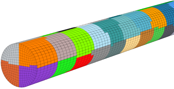
(a) Partition

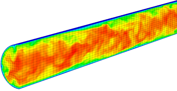
(b) Velocity magnitude

Figure 1: Partition of the elements on $64$ processes and velocity magnitude in the pipe ($Re_{\tau}=180$).

As it can be observed, solving the incompressible Navier-Stokes equations is reduced to the evaluation of $\mathbf{F}_{n}$ in Eq. (3), followed by one Poisson equation and a Helmholtz equation thereafter for each velocity component (2 in 2D and 3 in 3D). Eq. (4), the Poisson equation for the pressure, is the main source of stiffness and its efficient resolution by an iterative solver is preceded by two steps. First of all, the pressure at each time step is projected onto a subspace of previous solutions, and as described in [4] has been shown to reduce the iteration count by a factor $2.5-5$, which we also verify in Sect. 4. Then, a pressure preconditioner is built based on the additive overlapping Schwarz method, given by

$$M_{0}^{-1}:=R_{0}^{T}A_{0}^{-1}R_{0}+\sum_{k=1}^{K}R_{k}^{T}\tilde{A}_{k}^{-1}R_{k}.$$ (6)

The overlapping part requires local solves on each subdomain and is naturally parallelizable despite a fairly complex practical implementation [3, 6]. The coarse grid solve is in essence more difficult to parallelize and this can be performed in two different ways. The first method is a Cholesky factorization of the matrix $A_{0}^{-1}$ into $XX^{T}$ with a convenient refactoring of the underlying matrix to maximize the sparsity pattern of $X^{T}$. This factorization is subsequently referred to as XXT and details regarding complexity and implementation are available in [13]. The second method is a single V-cycle of a highly-tuned AMG solver that is designed specifically to be communication minimal and optimal for coarse-grid problems where one anticipates very few degrees of freedom per processor [10].

2.2 Implementation

2.2.1 Mesh and mapping

The geometry is meshed using hexahedral elements, partitioned for parallel computation using a spectral bisection algorithm as implemented in “genmap” which accompanies the code Nek5000 [2]. An example of the partitioning for the case $Re_{\tau}=180$ run on $64$ cores is shown in Fig. 1(a), where each element is colored according to the MPI rank it belongs to. We note that the partitioning is done at the element level and not finer.

2.2.2 Code structure

The sequence of operations leading to the solution of the incompressible Navier–Stokes equations is summed up algorithmically in Algorithm 1. First of all, note that both Eq. (4) and Eq. (5) can be summed up in discrete form as

$$H\phi=(h_{1}A+h_{2}B)[\phi],$$

where $A$ is the stiffness matrix stemming from the discretization of the Laplacian and $B$ is the mass matrix. Different choices for the factors $h_{1}$ and $h_{2}$ yield either the Poisson equation, or the Helmholtz equation

$$Hp = (A)[p]=f_{p},\quad(h_{1}=1,h_{2}=0)$$ (7)

$$Hu = (\frac{1}{Re}A-\frac{b_{0}}{\Delta t}B)[u]=f_{u},\quad(h_{1}=1,h_{2}=-\frac{b_{0}}{\Delta t}).$$ (8)

procedure Solver

     for k=1,…,nsteps do

         # Compute Pressure

         $f_{p}\leftarrow rhs_{p}(u,\mathbf{f})$

         $\delta f_{p}\leftarrow f_{p}-\text{proj}_{X_{f_{p}}}(f_{p})$

         $\delta p\leftarrow\text{Helmholtz}(H_{p},\delta f_{p})$

         $p\leftarrow p+\delta p$

         $X_{p}\leftarrow\left\{X_{p},\text{proj}_{X_{p}}(p)\right\}$

         $X_{f_{p}}\leftarrow\left\{X_{f_{p}},\text{proj}_{X_{f_{p}}}(H_{p}p)\right\}$

         # Compute Velocity

         $f_{u}\leftarrow rhs_{u}(p,u,\mathbf{f})$

         $\delta f_{u}\leftarrow f_{u}-\text{proj}_{X_{f_{u}}}(f_{u})$

         $\delta{u}\leftarrow\text{Helmholtz}(H_{u},\delta f_{u})$

         ${u}\leftarrow u+\delta u$

         $X_{u}\leftarrow\left\{X_{u},\text{proj}_{X_{u}}(u)\right\}$

         $X_{r_{u}}\leftarrow\left\{X_{f_{u}},\text{proj}_{X_{f_{u}}}(H_{u}u)\right\}$      

Algorithm 1 Main solver.

By virtue of the method of projections, we do not solve $Hp=f_{p}$ or $Hu=f_{u}$, but rather $H\delta p=\delta f_{p}$ and $H\delta u=\delta f_{u}$, where $\delta f_{p}$ and $\delta f_{u}$ are the rejections of $f_{p}$ and $f_{u}$ respectively. Details on the technicalities of this are abundant in [4]. The first step is to compute the corresponding right hand sides and then project them onto a subspace of previous solutions (subspaces are denoted by $X$ and the size of the space is $L$). The corrections $\delta p$ and $\delta u$ are then computed by solving the Helmholtz equation for the rejections and added to the previous solution. A simplified structure for the Helmholtz solver is shown in Algorithm 2. The Poisson equation for the pressure is solved with the GMRES method. The pressure solve also includes the computation of the preconditioner based on the Schwarz overlapping method and coarse grid solve, which is not the case for the velocity and constitutes an important part of the work and communication. The Helmholtz equation is solved using the CG method for each component of the velocity.

procedure Helmholtz($H,r$)

     if Velocity then

         $x\leftarrow CG(H,r)$

     else if Pressure then

         $\left(M_{0}^{-1}\right)_{\text{Sch}}\leftarrow$ Overlapping Schwarz()

         $\left(M_{0}^{-1}\right)_{\text{cgs}}\leftarrow$ Coarse grid solve()

         $M_{0}^{-1}\leftarrow\left(M_{0}^{-1}\right)_{\text{Sch}}+\left(M_{0}^{-1}\right)_{\text{cgs}}$

         $x\leftarrow GMRES(M_{0}^{-1},H,r)$      

     return x

Algorithm 2 Helmholtz solver.

3 Benchmarking

3.1 Hardware

The test cases were run on three different supercomputers, namely Mira from the Argonne National Laboratory, USA, Titan from the Oak Ridge National Laboratory, USA, and Beskow from the PDC Center for High Performance Computing, KTH, Sweden. A quick overview of the characteristics of each computer is summarized in Tab. 1.

Table 1: Overview of the characteristics of the different supercomputers.

	System arch.	Core arch.	Number of cores	Cores/node	Topology	Processes/core
Mira	IBM BG/Q	PowerPC A2	$786,432$	$16$	5D torus	2
Titan	Cray XK7	AMD Opteron	$299,008$	$16$	3D torus	1
Beskow	Cray XC40	Intel Haswell	$53,632$	$32$	DragonFly	1

The systems vary from small to large petascale and are meant to establish an overview of the Nek5000 scaling. On Mira, Nek5000 achieves its maximum performance when run with two processes per BG/Q core, being 32 processes per node which was noted already in [5]. Although Titan is a machine aimed at hybrid parallelism using graphics processing units (GPUs), which Nek5000 supports marginally as mentioned in [11], no production runs were performed outside the MPI environment and we shall restrict the use of Titan to CPU parallelism and rely solely on the 16 Opteron cores per node with one process each. The same setup of 1 process per CPU core, i.e. not using hyperthreading, was applied to the smallest system Beskow, a Cray XC40. Indeed, some tests performed on a single Haswell core showed that hyperthreading did not improve time to solution.

Table 2: Overview of the latencies and bandwidths. A word (wd) is 64 bits long.

	$\alpha^{*}(\mathrm{\mu s})$	$\beta^{*}(\mathrm{\mu s/wd})$	$t_{a}(\mathrm{\mu s})$	$\alpha$	$\beta$
Mira	$4$	$5\cdot 10^{-3}$	$1.1\cdot 10^{-3}$	$3600$	$5$
Titan	$2.25$	$1.42\cdot 10^{-3}$	$6.5\cdot 10^{-4}$	$3500$	$2.2$
Beskow	$2.55$	$8.25\cdot 10^{-4}$	$1.5\cdot 10^{-4}$	$17000$	$5.5$

In order to assess the performance of the machines at hand, we computed some of the network characteristics that determine the communication. In particular Beskow, which is a relatively new machine, had no such parameters provided to users. The performance study conducted here relies on the linear interprocessor communication model

$$t_{c}(m)=(\alpha+\beta m)t_{a},$$ (9)

where $t_{c}$ is the communication time, $m$ is the message length (number of 64-bit words) and $t_{a}$ is the inverse of the observed flop rate. The relevant quantities here are $\alpha$ and $\beta$, the non-dimensional latency and inverse bandwidth. We denote by $\alpha^{*}$ and $\beta^{*}$ the corresponding dimensional latency and inverse bandwidth. The relation between dimensional and non-dimensional parameters is given by

$$\alpha=\frac{\alpha^{*}}{t_{a}}\qquad\text{and}\qquad\beta=\frac{\beta^{*}}{t_{a}}.$$

The values of $\alpha^{*}$ and $\beta^{*}$ are computed following a “ping-pong" test as described in [5]. During this test, the time required to send and receive messages of various sizes between 512 processors (default value for the test in Nek5000) is measured and subsequently the values of $\alpha$ and $\beta$ are computed as the best fit for the linear model Eq. (9). The value of $t_{a}$ is determined by performing a number of matrix-matrix multiplications streamed from memory representing the tensor products that are at the core of a spectral element solver [1] and accounting for a big part of the solve time [8]. The tensor products considered imply 3D elements with polynomial order ranging from $10$ to $13$. Three different interpretations of the memory layout for the matrices are considered leading to a total of $12$ tests. For each test, the time and number of operations are measured and flop rate is computed. Data are then averaged and $t_{a}$ is taken as the inverse of the mean flop rate. Results for the ping-pong test are shown in Fig. 2 along with the linear model for all computers. An overview of the latencies, bandwidths and inverse flop rates is presented in Tab. 2. The non-dimensional parameters $\alpha$ and $\beta$ are a relative measure of the communication to computation cost. High values for these parameters imply that the limitation in parallel efficiency will arise earlier due to a relatively high communication cost. Consistent throughout all our studies is that all machines are strongly limited by the latency, already a noted common feature of modern computers. This limitation is strongest on Beskow, which is the newest of the three machines and has fastest CPUs. Therefore, it is expected that Beskow will not scale as well as the two others.

A drawback of our performance model is that it does not capture system noise. Furthermore, it assumes that all communication between two processes is homogeneous; it does not distinguish for example between on node and off node communication. This model works well for Mira. This work will also point out its weakness when dealing with system noise. For a better understanding of the impact of system noise, a relevant discussion about noise at scale can be found in [7].

As a side note, hardware might not be the only responsible for the high noise in communication and we would like to mention as an indication that we used the Cray programming environment version $5.2.26$.

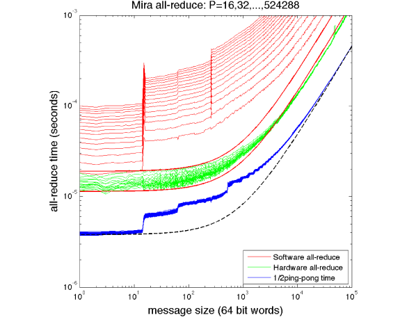
(a) Ping-pong and all-reduce on Mira as illustrated in [5]

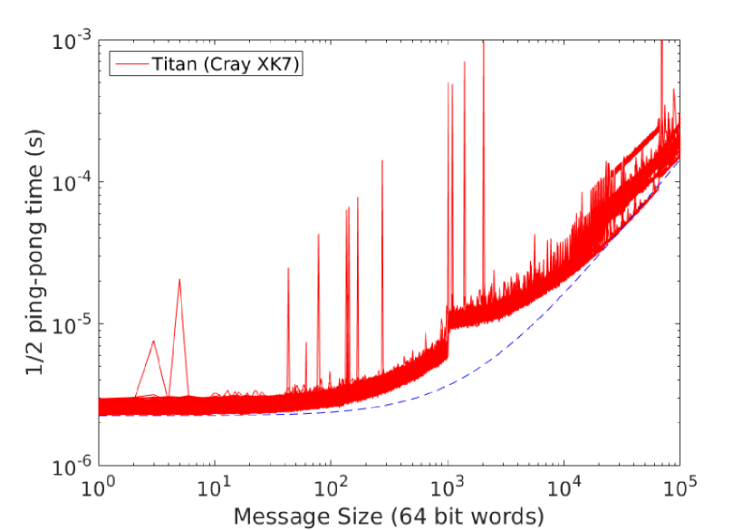
(b) Ping-pong on Titan

(c) Ping-pong on Beskow

Figure 2: Latency and bandwidth tests.

3.2 Code instrumentation for profiling

We assess the scalability and parallel efficiency of Nek5000 by studying the distribution between the time spent in communication and the time spent in computation for each simulation. These measurements are performed with performance tools adapted to each computer. The tools are set to start counting after the initial setup stage is completed, in our case after timestep 30, lasting for an extra 20 timesteps. The initial stage is meant to allow for the high-order restart, proper initialization of the projection space (i.e. the size of the projection space $X$ is $L=5$, thus requiring 5 consecutive solutions). In order to measure the time spent in communication we relied on Craypat for Beskow and Titan and on Hardware Performance Monitor (HPM) for Mira. Both tools allow us to measure the total time spent in communication during the targeted 20 time steps. HPM gives additional information on the cache misses and the load imbalance. The CrayPat performance analysis framework is used to sample the code during execution at a default frequency of $100\,\mathrm{Hz}$ and reports in which function each sample was taken. Then, we assume that the proportion of the total time spent in a given function is equal to the proportion of samples within this function. The sampling procedure ensures a very low overhead. We also tested the tracing procedure, where all function calls are traced, available with Craypat but overhead in time was about $50\%$ and the method was abandoned.

3.3 Test case : pipe flow

The test case considered is the turbulent flow in a straight pipe. A thorough description of the flow configuration as well as a detailed analysis of the physical results can be found in [9]. The flow was run at four different friction Reynolds numbers $Re_{\tau}=180$, $360$, $550$ and $1000$. A summary of the different simulations and associated number of elements, polynomial order and number of grid points $N$ is presented in Tab. 3. The friction Reynolds number is defined as $Re_{\tau}=u_{\tau}R/\nu$, where $u_{\tau}$ is the friction velocity, $R$ is the radius of the pipe and $\nu$ is the kinematic viscosity. The bulk Reynolds number is defined as $Re_{b}=2U_{b}R/\nu$, where $U_{b}$ is the mean bulk velocity. A pressure gradient is imposed inside the pipe through a forcing term and periodic boundary conditions are imposed at the inlet and the outlet. A snapshot of the velocity magnitude for the case $Re_{\tau}=180$ is illustrated in Fig. 1(b).

Table 3: Summary of the different pipe flows configurations.

$Re_{\tau}$	$Re_{b}$	# elements	pol. order	# grid points
$180$	$5300$	$36,480$	$8$	$18.67\times 10^{6}$
$360$	$11,700$	$237,120$	$8$	$121.4\times 10^{6}$
$550$	$19,000$	$823,632$	$8$	$437.0\times 10^{6}$
$1000$	$37,700$	$1,264,032$	$12$	$2.184\times 10^{9}$

4 Performance and Scaling Analysis

Our abstraction assumes that large scale runtime performance is mainly composed of

1. system hardware parameters consisting of the network topology, latency and bandwidth, and flops per second of matrix matrix products (usually memory bandwidth bound),

2. time $T_{a}$ and $T_{c}$ spent in computation and communication for the measured $20$ timesteps largely dependent on point 1 and on their respective algorithmic complexities,

3. partitioning.

The partitioning for our test case (see Sect. 3.3) is considered to be topologically equivalent to a cube. The resulting runtime complexities are extensively described in [5] for the Mira system. Based on these theoretical results we use profiling tools and wall clock timers to measure the load imbalance, cache misses, as well as weak and strong scaling. Load imbalance and cache misses are only measured on Mira via the HPM profiling library. We want in particular to verify experimentally the strong scaling limit for a given problem of size $N$. In this paper, the strong scaling limit for a problem of size $N$ is defined as the minimal number of grid points per process $\frac{N}{P}$ by finding $P$, the number of processes, such that

$$\dfrac{T_{a}(N,P)}{T_{c}(N,P)}=1,\mbox{ for problem size }N.$$ (10)

Alternatively, the strong scaling limit is commonly described by the derivative $\frac{dT}{dP}$ of the total time $T(N,P)$ being equal to $0$, i.e. the point where the runtime starts increasing again with increasing $P$. That point represents the fastest time to solution. This is rather an upper bound of the strong scaling limit that would in most of our test runs never be observed. For Nek5000 on Mira it has little practical meaning to the user, as that limit always implies the usage of all of Mira, which is in most cases too costly. Without a cost model, Eq. (10) gives us a much lower and practical bound of the strong scaling limit. If communication takes longer than computation, the code is deemed to be at the strong scaling limit where the scaling starts diverging significantly from the perfect linear scaling.

The test case used to explore the scaling behavior of Nek5000 is the one of a turbulent flow in a straight pipe, a generic and widely known case across the CFD community. This should allow potential users to estimate and compare the scaling of Nek5000 to other CFD software. Our test case is run in four different regimes for 4 different problem sizes denoted by $Re_{\tau}=180$, $360$, $550$ and $1000$, described more in detail in Sect. 3.3. These cases were run with various processor counts on three systems. The lower bound of the processor count is dictated by the size of the random access memory (RAM) of each machine, i.e. the smallest number of nodes on which the problem can be packed. Nek5000 has roughly a memory requirement of 500 fields times the number of degrees of freedom. The upper bound was either set by the administrative limit of getting access to the maximum number of processors (Beskow and Titan) or by the algorithmic limit of having at least one element per process, since as noted in Sect. 2.2.2, the smallest parallelizable unit in Nek5000 is one spectral element. Of the 20 timesteps along which the statistics are taken we consider the mean communication time reported over all processes.

In [5] the strong scaling limit Eq. (10) was estimated to be around $\frac{N}{P}=2000$ for the conjugate gradients (CG) and $7000$ for the geometric multigrid (MG) on Mira when using finite differences. These values are given as an indication but we remind that Nek5000 is an incompressible flow solver and gathers several different algebraic solvers each with its own customized preconditioning strategy. Indeed CG is implemented with Jacobi preconditioning for velocity and GMRES is used with XXT and AMG (which is different from the geometric multigrid) preconditioning for pressure. Taking also the added computational effort from projections, right hand side evaluations and the heavy communication of the coarse grid solver our values deviate slightly from the theoretical results in [5].

5 Results

The core of the present analysis relies on the data in Fig. 3, Fig. 4 and Fig. 5 for each one of the three machines discussed here. The compute time and communication time are illustrated along with the total time for both XXT and AMG across all test cases. Since each independent measurement is taken at powers of $2$ number of processes $P$ the plots are presented in logarithmic scale. However, in order to help identify linear scaling of the compute time, the optimal linear scaling line of the compute time was added, i.e.

$$T_{ideal}(N,P)=\frac{T(N,P_{1})P_{1}}{P}$$

where $P_{1}$ is the lowest process count possible for the given problem size. It is noteworthy that we do not compare to linear scaling of the total time as we operate in the strong scaling limit regime, where parallel efficiency is supposed to be well below unity.

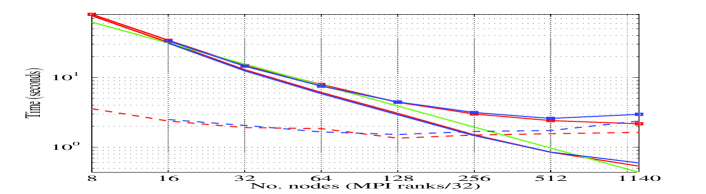
(a) $Re_{\tau}=180$

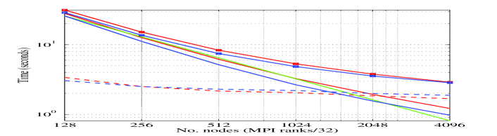
(b) $Re_{\tau}=360$

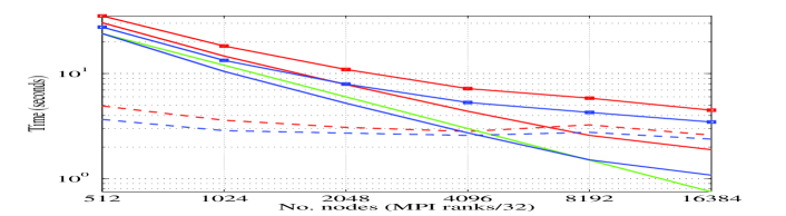
(c) $Re_{\tau}=550$

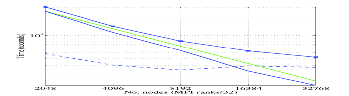
(d) $Re_{\tau}=1000$

Figure 3: Total time for 20 timesteps on BG/Q Mira: AMG (blue), XXT (red), communication (dashed), computation (solid), total time ($\square$), computational linear scaling (green).

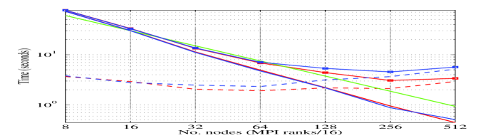
(a) $Re_{\tau}=180$

(b) $Re_{\tau}=360$

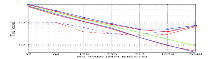
(c) $Re_{\tau}=550$

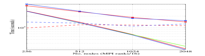
(d) $Re_{\tau}=1000$

Figure 4: Total mean time for 20 timesteps on Titan: AMG (blue), XXT (red), communication (dashed), computation (solid), total time ($\square$), computational linear scaling (green).

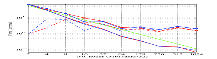
(a) $Re_{\tau}=180$

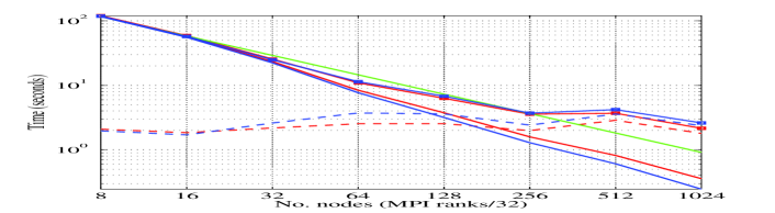
(b) $Re_{\tau}=360$

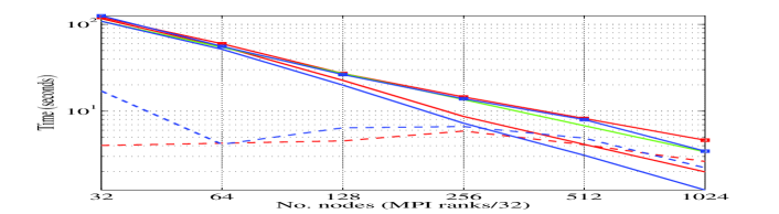
(c) $Re_{\tau}=550$

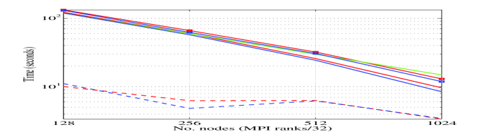
(d) $Re_{\tau}=1000$

Figure 5: Total mean time for 20 timesteps on Beskow: AMG (blue), XXT (red), communication (dashed), computation (solid), total time ($\square$), computational linear scaling (green).

5.1 Strong scaling limit

For both XXT and AMG the strong scaling limit, i.e. Eq. (10), can be readily extracted from the plots by examining the intersection of the computation time and the communication time. For the given intersection point we can identify the values of $\frac{N}{P}$ through linear interpolation and they are reported them in Tab. 4.

Table 4: Strong Scaling Limit for all 4 test cases on Beskow, Titan and Mira in degrees of freedom per core $\frac{N}{P}$ with 2 processes per core on Mira, 1 process per core on Beskow and Titan.

Mira	$Re_{\tau}180$	$Re_{\tau}360$	$Re_{\tau}550$	$Re_{\tau}1000$
XXT	4496	3412	4192	-
AMG	5040	5578	6200	9750
Titan	$Re_{\tau}180$	$Re_{\tau}360$	$Re_{\tau}550$	$Re_{\tau}1000$
XXT	9000	24000	65000	228000
AMG	11000	36000	68000	132000
Beskow	$Re_{\tau}180$	$Re_{\tau}360$	$Re_{\tau}550$	$Re_{\tau}1000$
XXT	45700	19200	26000	-
AMG	24800	33000	48000	-

In practice we observed a strong scaling limit for XXT at roughly $1900<\frac{N}{P}<2300$ and for AMG at $2300<\frac{N}{P}<4000$ on Mira, below the $7000$ anticipated in [5].

On Beskow, the scalability limit is more difficult to locate with confidence due to the high variance in communication times (see Fig. 2(c)), in particular for small cases. Nevertheless we present it given in Fig. 5, while keeping in mind that this is the result of a single run and not averaged across several samples. The scalability limit on Beskow is roughly one order of magnitude higher than on Mira in terms of degrees of freedom per core and is located around $\frac{N}{P}\sim 20,000-50,000$. This is consistent with the values for the non-dimensional latency $\alpha$ from Tab. 2. Indeed Beskow has faster CPUs, thus having a lower value for $t_{a}$. This leads to a higher $\alpha$, although the values for $\alpha*$ are relatively comparable for Titan, Mira and Beskow.

As an intermediate conclusion, we note that the scalability limit on Mira and Beskow is almost independent of the problem size and number of cores that are used.

On Titan, the scalability limit exhibits a different behavior. The strong scaling limit for $\frac{N}{P}$ increases significantly with bigger cases as we see from Tab. 4. The limit goes from $\frac{N}{P}\sim 9000$ to $\frac{N}{P}\sim 228,000$ across the cases $Re_{\tau}=180$ to $Re_{\tau}=1000$ for XXT. Similarly for AMG $\frac{N}{P}\sim 11,000$ increases sharply to $\frac{N}{P}\sim 132,000$ from the smallest case $Re_{\tau}=180$ to $Re_{\tau}=1000$. This limitation cannot be fully explained from the non-dimensional latencies and bandwidths from Tab. 2.

The first plausible explanation is the occasional, random latency spikes seen in the ping-pong tests. If one process experiences this, the created imbalance has repercussions for all processes in a parallelized CFD code. We see that these spikes increase communication by an order of magnitude or higher. The more compute nodes are involved, the higher the risk of a latency spike. This may partially explain Titan’s strong scaling limit in grid points per process $\frac{N}{P}$ increase with increasing $P$.

Secondly the ping-pong test used to compute the parameters $\alpha$ and $\beta$ is performed on $512$ cores only. During this test, the cores are very likely to lie close to each other on the computer. However, this ideal situation does not hold any more when a high number of cores is considered, as they are probably split on many remote nodes. A poor interconnect network between cabinets or a high network load on Titan could be a valid reason for the observed deterioration and an analysis based on the linear communication model given by $\alpha$ and $\beta$ becomes irrelevant on Titan at a high core count.

5.2 Super-Linearity

In theory the computational time should match exactly the linear scaling as work is distributed according to the ratio $\frac{N}{P}$.

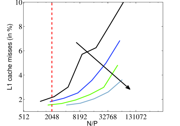
Figure 6: Cache misses on Mira for all 4 test cases (low to high degrees of freedom in direction of the arrow). Percentage of load operations for data and instructions. Dashed red line: L1 cache size.

All test cases on all the systems show a super-linear scaling. This observation holds true with all timers and profilers switched off.

The usual explanation for super-linear scaling is a sudden decrease of the cache misses for decreasing $\frac{N}{P}$, as parts of the solver can entirely work on data that lies in the cache. To investigate this, we extracted the cache misses on Mira as provided through HPM by accessing hardware counters (see Fig. 6). Mira is equipped with both a L1 data cache and instruction cache of 16kB each. The cache misses account for both data and instruction cache misses. The L2 cache of 32MB, that is located at the node level, becomes irrelevant as HPM consistently reported over 97% cache misses. The L1 cache can be filled with $2048$ double precision numbers, see Fig. 6 the vertical dashed red line which indicates the cache size of 16kB below which all gridpoints would theoretically fit into data cache. As we run with 2 processes per core, this would be at roughly $1000$ degrees of freedom per process. Although the data fields achieve those sizes only at the strong scaling limit we do observe a general decrease in cache misses with decreasing $\frac{N}{P}$ and thus a better cache exploitation. We cannot explain this behavior as that would require a more granular analysis of the computational kernels. Measuring the cache misses over the entire timestep with mixed data and instruction misses, gives us only a general overview of the cache behavior. In summary, we attribute the super-linear scaling to cache management and pipelining on the CPU of Mira. We do not possess profiling results for Beskow or Titan and cannot study the cache misses there but we assume that the reason for super-linearity is similar as for Mira.

5.3 Comparison between XXT and AMG

For smaller problem sizes ($Re_{\tau}=180$), XXT slightly outperforms AMG on all machines for a large number of cores, after the strong scaling limit has been reached. For this case, computation time is almost unaffected by the method and the better perfomance of XXT is attributed to a lower communication. For the cases $Re_{\tau}=360$ and $550$ on Mira and Beskow, compute time is noticeably lower for AMG than XXT by about $5-10\%$. For $Re_{\tau}=550$ on Mira, computation time is also lower for AMG. This leads to the clear conclusion that AMG for this case on this computer is systematically better by about $10\%$. However, no such incisive conclusion can be drawn for the other cases because of varying communication times. For $Re_{\tau}=1000$ on Beskow, AMG is once again faster in terms of computation and communication time, but the gain is hardly a few percents and we are still far from the strong scaling limit. On Titan, the difference between AMG and XXT is marginal even if AMG seems overall slightly slower.

Interesting data are the total number of MPI calls and associated message length for both methods. In Tab. 5 we compare XXT and AMG on $Re_{\tau}=550$ at the strong scaling limit of AMG (4096 nodes). The amount of data communicated by XXT is by an order of magnitude higher, while AMG uses twice as many MPI calls. Therefore, AMG should leap ahead if the systems rely on a low latency network combined with a high element count.

Table 5: Number of MPI calls and data communicated on $P=131,072$ at $Re_{\tau}=550$.

	AMG		XXT
MPI Routine	#calls	bytes	#calls	bytes
MPI_Isend	96638	360.5	62336	6363.8
MPI_Irecv	96638	362.7	5916	61885.4
MPI_Waitall	38971	0.0	56420	542.0
MPI_Allreduce	10956	5921.0	5848	10.0
Total	252312		130520

5.4 Load balancing

Beyond the strong scaling limit, the computation time increases and approaches the linear scaling line again. This is attributed to the load imbalance as in the extreme case some processes have to work on one element and some processes on two elements. This can be observed in Fig. 7 where the imbalance for $Re_{\tau}=1000$ on 32,768 nodes creates two spikes in the distribution of the execution time. The histogram includes the imbalance of the workload as well as the resulting imbalance in the communication.

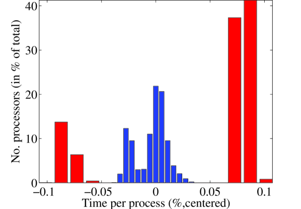
Figure 7: Histogram of the load imbalance at $2.184\times 10^{9}$ degrees of freedom: number of processes per time spent in communication. Red bins: % of processes at the lowest per core load, blue bins: % of processes at highest per core load.

5.5 Weak scaling

As a byproduct of our analysis we can mimic a weak scaling analysis by stacking up all problem sizes at every MPI rank count. On Mira the communication is mostly latency bound with a small influence from the bandwidth. This holds also true for peer to peer communication as well as for the all-reduce (see Fig. 2). Across the four test cases we can observe a weak scaling in Fig. 8. It proves that the scaling on Mira is mainly dependent on the ratio $\frac{N}{P}$.

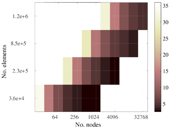
Figure 8: Weak Scaling: For a fixed $\frac{N}{P}$, the same runtime is observed across the four test cases, colorbar : total time (seconds).

5.6 Time to solution

Although we focus on parallelism and performance across a high number of processes the most important feature of a CFD code remains, in practice, the ability to minimize the time to solution. The parallelsim is not the sole contributor to fast time to solution, but also secondary strategies such as projections mentioned in Sect. 2.1. Here we assessed a recent upgraded implementation of the projections scheme, see Fig. 9, where we note that the number of iterations per solve decreases around 3.5 times as we increase the projections space $L$. Compared to the reported results in [4] an improved reusability of the projection space data eliminates the spikes in convergence. As we mentioned before, the memory footprint of Nek5000 is roughly 500 fields. Thus the additional memory requirement of the projections is currently of little relevance.

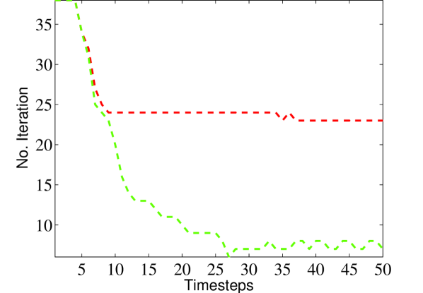
Figure 9: Convergence of solution with increase of projections space $L$ (green: $L=5$, red $L=0$).

6 Conclusion

Our four test cases from 18 million to 2 billion degrees of freedom were successfully run on three different petascale system architectures from the lowest, memory bound, processor count to the granularity limit in order to assess the strong scaling of Nek5000. We can confirm on Mira that we can match the theoretical limits established in [5]. However on the Cray systems we observed one to two orders of magnitude lower strong scaling limits due to higher latency and high noise across the network. Our results point at the regimes under which to choose AMG or XXT; AMG for low latency and high element count, XXT for high latency, high bandwidth and low element count. The linear communication model proved itself insuficient for explaining the difference in the strong scaling limit between Titan and Mira. Including a quantity for the network noise may improve scaling predictions on noisy systems. We confirmed that a synchronized and low latency global communication remains crucial for strong scaling of a spectral element based CFD solver.

7 Acknowledgments

This research used resources provided by the Swedish National Infrastructure for Computing (SNIC) at PDC Centre for High Performance Computing (PDC-HPC). This research used resources of the Argonne Leadership Computing Facility, which is a DOE Office of Science User Facility supported under Contract DE-AC02-06CH11357. This research used resources of the Oak Ridge Leadership Computing Facility at the Oak Ridge National Laboratory, which is supported by the Office of Science of the U.S. Department of Energy under Contract No. DE-AC05-00OR22725. This research used resources of the Argonne Leadership Computing Facility, which is a DOE Office of Science User Facility supported under Contract DE-AC02-06CH11357. We thank Scott Parker and Kevin Harms from ALCF at Argonne for their invaluable suggestions and insights into performance analysis on Mira. We also thank the Nuclear Energy Advanced Modeling and Simulation (NEAMS) program and the Linné FLOW Center that funded part of this research.

The submitted manuscript has been created by the University of Chicago as Operator of Argonne National Laboratory (“Argonne”) under Contract No. DE-AC02-06CH11357 with the U.S. Department of Energy. The U.S. Government retains for itself, and others acting on its behalf, a paid-up, nonexclusive, irrevocable worldwide license in said article to reproduce, prepare derivative works, distribute copies to the public, and perform publicly and display publicly, by or on behalf of the Government.

References

- [1] M. O. Deville, P. F. Fischer, and E. H. Mund. High-Order Methods for Incompressible Fluid Flow. Cambridge University Press, 2002. Cambridge Books Online.
- [2] P. Fischer, J. Lottes, S. Kerkemeier, O. Marin, K. Heisey, A. Obabko, E. Merzari, and Y. Peet. Nek5000: User’s manual. Technical Report ANL/MCS-TM-351, Argonne National Laboratory, 2015.
- [3] P. F. Fischer. An overlapping schwarz method for spectral element solution of the incompressible Navier-Stokes equations. Journal of Computational Physics, 133(1):84 – 101, 1997.
- [4] P. F. Fischer. Projection techniques for iterative solution of Ax = b with successive right-hand sides. Computer Methods in Applied Mechanics and Engineering, 163(1-4):193–204, 1998.
- [5] P. F. Fischer, K. Heisey, and M. Min. Scaling Limits for PDE-Based Simulation (Invited). AIAA Aviation. American Institute of Aeronautics and Astronautics, jun 2015. doi:10.2514/6.2015-3049.
- [6] P. F. Fischer and J. W. Lottes. Domain Decomposition Methods in Science and Engineering, chapter Hybrid Schwarz-Multigrid Methods for the Spectral Element Method: Extensions to Navier-Stokes, pages 35–49. Springer Berlin Heidelberg, Berlin, Heidelberg, 2005.
- [7] T. Hoefler, T. Schneider, and A. Lumsdaine. Characterizing the influence of system noise on large-scale applications by simulation. In Proceedings of the 2010 ACM/IEEE International Conference for High Performance Computing, Networking, Storage and Analysis, SC ’10, pages 1–11, Washington, DC, USA, 2010. IEEE Computer Society.
- [8] M. Hutchinson, A. Heinecke, H. Pabst, G. Henry, M. Parsani, and D. Keyes. Efficiency of high order spectral element methods on petascale architectures. ISC High Performance, 2016.
- [9] G. K. Khoury, P. Schlatter, A. Noorani, P. F. Fischer, G. Brethouwer, and A. V. Johansson. Direct numerical simulation of turbulent pipe flow at moderately high Reynolds numbers. Flow, Turbulence and Combustion, 91(3):475–495, 2013.
- [10] J. Lottes. Independent quality measures for symmetric algebraic multigrid components. Argonne National Laboratory, Mathematics & Computer Science Division, 2005.
- [11] M. Otten, J. Gong, A. Mametjanov, A. Vose, J. Levesque, P. Fischer, and M. Min. An mpi/openacc implementation of a high-order electromagnetics solver with gpudirect communication. International Journal of High Performance Computing Applications, 2016.
- [12] A. G. Tomboulides, J. C. Y. Lee, and S. A. Orszag. Numerical simulation of low Mach number reactive flows. Journal of Scientific Computing, 12(2):139–167, 1997.
- [13] H. Tufo and P. Fischer. Fast parallel direct solvers for coarse grid problems. Journal of Parallel and Distributed Computing, 61(2):151 – 177, 2001.
- [14] H. M. Tufo and P. F. Fischer. Terascale spectral element algorithms and implementations. In Proceedings of the 1999 ACM/IEEE Conference on Supercomputing, SC ’99, New York, NY, USA, 1999. ACM.