RAVE J203843.2$-$002333 (catalog ): The First Highly R-process-Enhanced Star
Identified in the RAVE Survey.

Abstract

We report the discovery of RAVE J203843.2$-$002333 (catalog ), a bright ($V=12.73$), very metal-poor ($[\mathrm{Fe}/\mathrm{H}]$ = $-$2.91), r-process-enhanced ($[\mathrm{Eu}/\mathrm{Fe}]$ = $+$1.64 and $[\mathrm{Ba}/\mathrm{Eu}]$ = $-$0.81) star selected from the RAVE survey. This star was identified as a metal-poor candidate based on its medium-resolution ($R\sim 1,600$) spectrum obtained with the KPNO/Mayall Telescope, and followed-up with high-resolution ($R\sim 66,000$) spectroscopy with the Magellan/Clay Telescope, allowing for the determination of elemental abundances for 24 neutron-capture elements, including thorium and uranium. RAVE J2038$-$0023 (catalog ) is only the fourth metal-poor star with a clearly measured U abundance. The derived chemical-abundance pattern exhibits good agreement with those of other known highly r-process-enhanced stars, and evidence in hand suggests that it is not an actinide-boost star. Age estimates were calculated using Th/X and U/X abundance ratios, yielding a mean age of $13.0\pm 1.1$ Gyr.

1 Introduction

Advances in observations and theory in the past few years are converging on identifying the likely astrophysical site(s) of the rapid neutron-capture process (r-process), some sixty years after it was first suggested to account for the production of roughly half of the heavy elements beyond iron (Burbidge et al., 1957; Cameron, 1957). The recent discovery of highly r-process-enhanced stars in the ultra-faint dwarf galaxy Reticulum II (Ji et al., 2016; Roederer et al., 2016) opens a new observational window on the origin of the r-process. The observed enhancements point to enrichment by a rare astrophysical event that copiously produces r-process elements. The presently favored site that fits these characteristics (high temperatures, densities, and flux of free neutrons on short timescales; Burbidge et al., 1957) is the outflow from binary neutron star mergers (NSMs; Meyer, 1989; Bauswein et al., 2013; Rosswog et al., 2014). This environment has been argued to be a possible source of the r-process since the work of Lattimer & Schramm (1974). If this hypothesis is correct, it would be possible to link all the r-process-enhanced stars observed to date (including those in the halo field) to a common formation site and/or class of parent progenitors, which would add important constraints to theoretical predictions for the chemical evolution of the Galaxy and the Universe. Other possible sites of the r-process, including the so-called magneto-rotational supernovae (MR-SNe), which address several concerns raised about NSMs as the single site (e.g., Cescutti et al. 2015; Tsujimoto & Nishimura 2015; Wehmeyer et al. 2015; Beniamini et al. 2016), are currently being explored (Nishimura et al., 2017).

Observations of stars in ultra-faint dwarf galaxies are challenging due to their faint magnitudes ($g\gtrsim 17$). Because of that, (brighter) field halo stars can provide more detailed information on the r-process element abundances, to help better constrain its origins. The modern era of detailed exploration of this question opened with the discovery of the highly r-process-enhanced star CS 22892-052 (Sneden et al., 1994), an extremely metal-poor star (originally identified in the HK Survey of Beers and collaborators; Beers et al., 1985, 1992) with r-process elemental-abundance ratios exceeding ten times the solar values. These stars are known as r-II stars ($[\mathrm{Eu}/\mathrm{Fe}]$ $>+1.0$ and $[\mathrm{Ba}/\mathrm{Eu}]$ $<0.0$; Beers & Christlieb, 2005). Other examples of such stars have been identified over the past few decades, as the result of dedicated searches (e.g., HERES, the Hamburg/ESO R-process Enhanced Star survey, see Christlieb et al., 2004; Barklem et al., 2005) and other large high-resolution spectroscopic studies of very metal-poor (VMP; $[\mathrm{Fe}/\mathrm{H}]$ $<-2.0$; Beers & Christlieb, 2005; Frebel & Norris, 2015) and extremely metal-poor (EMP; [Fe/H] $<-3.0$) stars in the Galactic halo (e.g., Cayrel et al., 2004; Roederer et al., 2014b), and now number on the order of 25 stars.

The remarkable agreement between the r-process-element pattern observed in r-II stars and the Solar System suggests that either the r-process elements were well-mixed into the interstellar medium, or more likely, that the production of r-process elements resulted from the contribution by a unique astrophysical site in the early Galaxy. Furthermore, suggestions that the r-process enhancement in stars could be the result of peculiarities in the atmospheres of evolved stars or associated with mass-transfer binaries have been disproven as a result of (i) The identification of r-process-enhanced stars in essentially all stages of stellar evolution (Roederer et al., 2014a) and (ii) The binary frequency of such stars revealed by long-term radial-velocity monitoring (18 $\pm$ 6 %; Hansen et al., 2015) being similar to the frequency of other halo stars lacking this signature (16 $\pm$ 4 %; Carney et al., 2003).

The identification of r-II stars requires high-resolution spectroscopy. Among the $\sim$25 r-II stars with published analyses (Suda et al., 2008; Frebel, 2010), the abundances of both thorium and uranium could only be measured in three cases (CS 31082-001; Hill et al. 2002, HE 1523-0901; Frebel et al. 2007, and CS 29497-004; Hill et al. 2016). The star BD+17^∘3248 ($[\mathrm{Eu}/\mathrm{Fe}]$ = $+0.9$; Cowan et al., 2002) is considered by the authors to have a tentative U detection. A higher quality spectrum of this star is needed to better constrain the U abundance. The abundances of radioactive isotopes of elements such as Th and U can also place constraints on the age of the Universe, and be used to validate their early production, within the first $\sim$0.5-1.5 Gyr following the Big Bang. Age estimates are obtained by application of the nucleo-chronometry technique, pioneered for metal-poor stars by Butcher (1987), using theoretical production ratios and abundance ratios of stable r-process elements and radioactive isotopes (e.g., ²³²Th, half-life $14.0$ Gyr, and ²³⁸U, half-life $4.5$ Gyr). In the case that both U and Th are measured in the star, the U/Th chronometer pair can be used (Cayrel et al., 2001; Hill et al., 2002, 2016).

Table 1: Observational Data

RAVE J2038$-$0023 (catalog )			Mayall	Magellan 2014	Magellan 2016	RAVE
$\alpha$ (J2000)	20:38:43.2	Date	2014 09 15	2014 09 25	2016 04 16	$\cdots$
$\delta$ (J2000)	$-$00:23:33	UT	02:19:52	04:17:03	08:46:14	$\cdots$
$V$ (mag)	12.73	Exptime (s)	600	900	5,400	$\cdots$
$B-V$	0.99	R	2,000	38,000	66,000	8,000
$g$ (mag)	13.32	Vr(km/s)	$-$332.9	$-$321.7	$-$321.6	$-$319.6
$g-r$	0.87	S/N (3860Å)	50	30	100	$\cdots$
$J$ (mag)	10.73	S/N (4550Å)	80	90	220	$\cdots$
$J-K$	0.41	S/N (7900Å)	$\cdots$	150	$\cdots$	$\cdots$

In this paper we report the discovery of the r-II star RAVE J203843.2$-$002333 (catalog ) (hereafter RAVE J2038$-$0023 (catalog ); $[\mathrm{Fe}/\mathrm{H}]$$=-2.91$), the fourth low-metallicity star where abundances of both Th and U could be confidently measured. This star was originally selected as a bright ($V=12.7$) VMP candidate from the RAVE (RAdial Velocity Experiment; Steinmetz et al., 2006) fourth data release (DR4; Kordopatis et al., 2013), and medium-resolution spectroscopy with the KPNO/Mayall telescope revealed that this target is indeed a low-metallicity giant without carbon enhancement. Subsequent high-resolution follow-up with the MIKE spectrograph on the Magellan/Clay Telescope confirmed the presence of enhancements in r-process elements, such as Ba, Eu, Th, and U, which are reported here.

This paper is outlined as follows. Section 2 describes the target selection for the medium-resolution spectroscopic investigation and the high-resolution follow-up observations, followed by the determinations of the stellar parameters in Section 3. Section 4 provides details on the abundance determinations. Section 5 discusses the r-process abundance pattern of RAVE J2038$-$0023 (catalog ) compared with other r-II stars, including those with previously detected U, and obtains age estimates for RAVE J2038$-$0023 (catalog ) based on selected chronometry pairs. Our conclusions and a brief discussion are provided in Section 6.

2 Target Selection and Observations

RAVE J2038$-$0023 (catalog ) was selected as a metal-poor candidate star from RAVE DR4, part of a sub-sample with $4500<T_{\mathrm{eff}}<5750$ and $[\mathrm{Fe}/\mathrm{H}]$ $<-1.8$. These targets were then followed up with medium-resolution spectroscopy on a variety of telescopes, in order to validate their atmospheric parameters and obtain carbon abundance estimates. High-resolution spectroscopic follow-up was then carried out for the most interesting candidates. The full description of the target selection and spectroscopic follow-up will be provided in a forthcoming paper.

2.1 Medium-Resolution Spectroscopy

Medium-resolution spectroscopic follow-up was carried out with the Mayall 4-m Telescope at Kitt Peak National Observatory. The observations were obtained in semester 2014B, using the R-C spectrograph, with the KPC007 grating (632 l mm^-1), the blue setting, a 1$\farcs$0 slit, and covering the wavelength range [3500,6000] Å. This combination yielded a resolving power of $R\sim 1,600$, and signal-to-noise ratio S/N $\sim 80$ per pixel at 4550  Å. The calibration frames included FeAr exposures (taken following the science observation), quartz-lamp flat-fields, and bias frames. All reduction tasks were performed using standard IRAF packages. Table 1 lists details of the observations from RAVE, and also the medium- and high-resolution spectroscopic follow-ups.

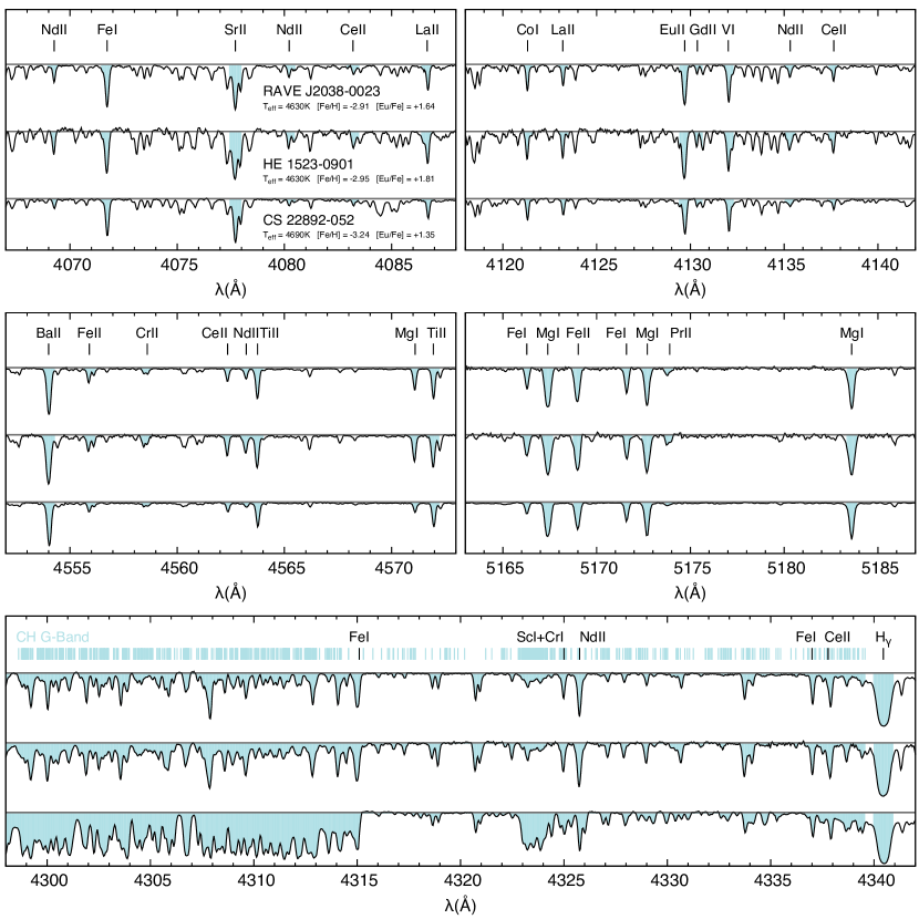
Figure 1: Selected regions of the spectrum of RAVE J2038$-$0023 (catalog ), compared with the r-II stars HE 1523$-$0901 (Frebel et al., 2007) and CS 22892$-$052 (Roederer et al., 2014b). The upper and middle panels show regions where absorption features of Fe, Mg, and neutron-capture elements are present. The lower panel shows the CH $G$-band, used for carbon abundance determinations.

2.2 High-Resolution Spectroscopy

High-resolution spectroscopic data were obtained during the 2014B and 2016A semesters, using the Magellan Inamori Kyocera Echelle (MIKE; Bernstein et al., 2003) spectrograph on the Magellan/Clay Telescope at Las Campanas Observatory. For the 2014B run, the observing setup included a $0\farcs 7$ slit with $2\times 2$ on-chip binning, yielding a resolving power of $R\sim 38,000$ (blue spectral range) and $R\sim 30,000$ (red spectral range), measured from the arc lamp spectral features. The S/N at $4550\,$Å is $\sim$90. MIKE spectra have nearly full optical wavelength coverage ([$\sim$3500,9000] Å). For the 2016A run, the observations were carried out using the $0\farcs 35$ slit with $2\times 2$ on-chip binning, yielding a resolving power of $R\sim 66,000$. The S/N at $3860\,$Å (close to the U spectral feature) is $\sim$100, and $\sim$220 at $4550\,$Å (near a prominent Ba II feature). The data were reduced using the data reduction pipeline developed for MIKE spectra, described by Kelson (2003). Figure 1 shows the spectrum of RAVE J2038$-$0023 (catalog ), compared with the r-II stars HE 1523$-$0901 ($T_{\mathrm{eff}}$=4630 K, $[\mathrm{Fe}/\mathrm{H}]$=$-2.95$, and $[\mathrm{Eu}/\mathrm{Fe}]$=$+1.81$; Frebel et al., 2007) and CS 22892$-$052 ($T_{\mathrm{eff}}$=4690 K, $[\mathrm{Fe}/\mathrm{H}]$=$-3.24$, and $[\mathrm{Eu}/\mathrm{Fe}]$=$+1.35$; Roederer et al., 2014b), in regions where absorption features of neutron-capture elements are present (upper and middle panels), as well as in the region of the molecular CH $G$-band feature (lower panel).

3 Stellar Parameters

3.1 Medium-Resolution Spectrum

The stellar atmospheric parameters ($T_{\mathrm{eff}}$, $\log\,g$, and [Fe/H]), and the carbon abundance from the medium-resolution spectrum were obtained using the n-SSPP, a modified version of the SEGUE Stellar Parameter Pipeline (SSPP; Lee et al., 2008a, b, 2013). The values for $T_{\mathrm{eff}}$, $\log\,g$, and $[\mathrm{Fe}/\mathrm{H}]$, determined from photometry, line-indices, and matching with a synthetic spectral library (see Beers et al., 2014, for further details), were used as first estimates for the high-resolution analysis. Results are listed in Table 2.

3.2 High-Resolution Spectra

From the high-resolution MIKE spectrum, we determined the stellar parameters spectroscopically (see details below), using the SMH software developed by Casey (2014). Equivalent-width measurements were obtained by fitting Gaussian profiles to the observed absorption lines within SMH. Table 3 lists the lines used in this work, their measured equivalent widths, and the derived abundance from each line. We employed one-dimensional plane-parallel model atmospheres with no overshooting (Castelli & Kurucz, 2004), computed under the assumption of local thermodynamic equilibrium (LTE).

Table 2: Derived Stellar Parameters for RAVE J2038$-$0023 (catalog )

	$T_{\mathrm{eff}}$(K)	$\log\,g$(cgs)	$[\mathrm{Fe}/\mathrm{H}]$	$\xi$(km/s)
RAVE (DR4)	4315 (105)	0.82 (0.40)	$-$2.17 (0.10)	$\cdots$
RAVE (DR5)	4502 (51)	1.18 (0.21)	$-$2.60 (0.14)	$\cdots$
RAVE-on	4801 (82)	1.49 (0.15)	$-$2.74 (0.07)	$\cdots$
KPNO	4655 (150)	0.85 (0.35)	$-$3.10 (0.20)	$\cdots$
Magellan	4630 (100)	1.20 (0.20)	$-$2.91 (0.10)	2.15 (0.20)

The effective temperature of RAVE J2038$-$0023 (catalog ) was determined by minimizing trends between the abundances of 202 Fe I lines and their excitation potentials, and applying the temperature correction to the photometric scale suggested by Frebel et al. (2013). The microturbulent velocity was determined by minimizing the trend between the abundances of Fe I lines and their reduced equivalent widths. The surface gravity was determined from the balance of the two ionization stages of iron, Fe I and Fe II. RAVE J2038$-$0023 (catalog ) also had its stellar atmospheric parameters determined from the moderate-resolution ($R\sim 8,000$) RAVE spectrum by Kordopatis et al. (2013). These values, together with our determinations from the medium- and high-resolution spectra, are listed in Table 2. For completeness, we also include the parameters from the most recent release, RAVE DR5 (Kunder et al., 2017), and also from the RAVE-on catalog (Casey et al., 2016).

There is very good agreement between the effective temperatures derived from the medium- and high-resolution spectra used in this work; the RAVE DR5 value is less than $\sim$150 K cooler. The surface gravities are all within 1$\sigma$, and the high-resolution and RAVE DR5 $\log g$ values are nearly identical. The surface gravity estimates from RAVE DR4 and KPNO ($\log\,g$ = 0.82 and 0.85 respectively) are expected to be similar, as both of these estimates come from isochrone matching, while the high-resolution estimate ($\log\,g$ = 1.20) was determined spectroscopically. The $[\mathrm{Fe}/\mathrm{H}]$ estimate from RAVE DR4 appear significantly higher than those reported from RAVE DR5 and the medium- and high-resolution results; the latter two of which are in good agreement with one another. The RAVE-on metallicity is in better agreement with our high-resolution estimate than either DR4 or DR5 from RAVE. However, despite the RAVE-on result having a reduced chi-squared value of 0.63, this star was excluded from the RAVE-on release because the RAVE pre-processing pipeline, SPARV, flagged RAVE J2038$-$0023 (catalog ) as being a star with much higher temperature ($T_{\mathrm{eff}}$$>$10,000 K).

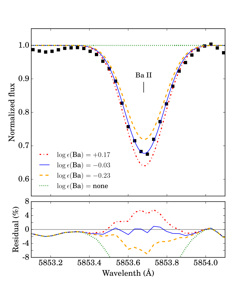
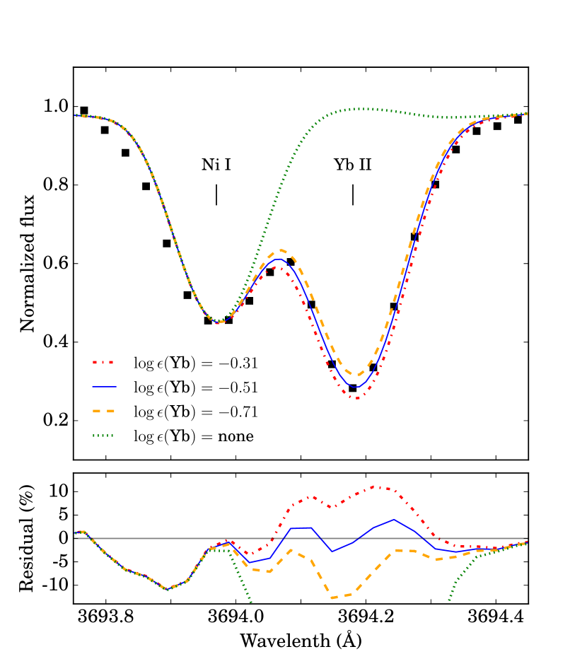
Figure 2: Observed spectra (squares) and synthesis (lines) for varying abundances of Sr II (left panel), Ba II (middle panel), and Yb II (right panel).

4 Chemical Abundances

Chemical abundances for RAVE J2038$-$0023 (catalog ) were calculated by equivalent-width analysis and spectral synthesis, using the MOOG code (July 2014 version; Sneden, 1973), which includes a proper treatment of scattering (see Sobeck et al., 2011, for details). The set of atmospheric parameters used for the abundance analysis is the one derived from the Magellan spectra. Tables 3 and 4 list the derived abundances for individual lines for light elements (C–Zn) and neutron-capture elements (Sr–U), respectively. The excitation potentials and oscillator strengths for the lines employed are taken from a variety of sources, including the compilations of Aoki et al. (2002), Barklem et al. (2005), and Roederer et al. (2012), as well as from the VALD database (Kupka et al., 1999) and the National Institute of Standards and Technology Atomic Spectra Database (NIST; Kramida et al., 2013). Elemental-abundance ratios, $[\mathrm{X}/\mathrm{Fe}]$, are calculated adopting solar photospheric abundances from Asplund et al. (2009). The average abundances for $39$ elements, derived from the Magellan/MIKE spectra, are listed in Table 5. The $\sigma$ values are the standard deviation and the $\overline{\sigma}$ are the standard error of the mean. For elements where $\overline{\sigma}$ is lower than 0.10, we adopt a fixed value of 0.10 (see discussion in Section 4.6 of Placco et al., 2013).

Uncertainties in the abundance determinations, as well as the systematic uncertainties due to changes in the atmospheric parameters, were treated using the same procedures described in Placco et al. (2013, 2015). Table 6 shows the changes in the derived chemical abundances due to variations (within the quoted uncertainties) in each atmospheric parameter. Also listed is the total uncertainty, calculated from the quadratic sum of the individual estimates. This calculation used only spectral features with abundances determined by equivalent-width analysis. The variations are $+$100 K for $T_{\mathrm{eff}}$, $+$0.2 dex for $\log\,g$, and $+$0.2 km s^-1 for $\xi$.

4.1 C to Zn

The carbon abundance for RAVE J2038$-$0023 (catalog ) was derived from the CH molecular feature at $\lambda$4313 ($[\mathrm{C}/\mathrm{Fe}]$ $=-0.44$). Since this star is on the upper red-giant branch, the measured carbon abundance does not reflect the chemical composition of its natal gas cloud. Using the procedure described in Placco et al. (2014a), we determined that the expected carbon depletion due to CN processing for RAVE J2038$-$0023 (catalog ) is 0.67 dex. Taking this into account, the corrected value for the carbon abundance is $[\mathrm{C}/\mathrm{Fe}]$ = $+0.23$. Abundances of Na, Mg, Al, Si, Ca, Sc, Ti, V, Cr, Mn, Co, Ni, and Zn were determined by equivalent-width analysis and spectral synthesis. Individual line determinations are listed in Table 3, and final abundances are provided in Table 5.

4.2 Neutron-Capture Elements

The chemical abundances for the neutron-capture elements were determined via spectral synthesis performed using MOOG. The results for individual lines are given in Table 4. Below we provide details on these measurements. Note that the uncertainty on individual synthesis measurements is typically set as $\pm$0.2 dex, as the measured abundance is well-bound between these limits (see, e.g., Figure 2).

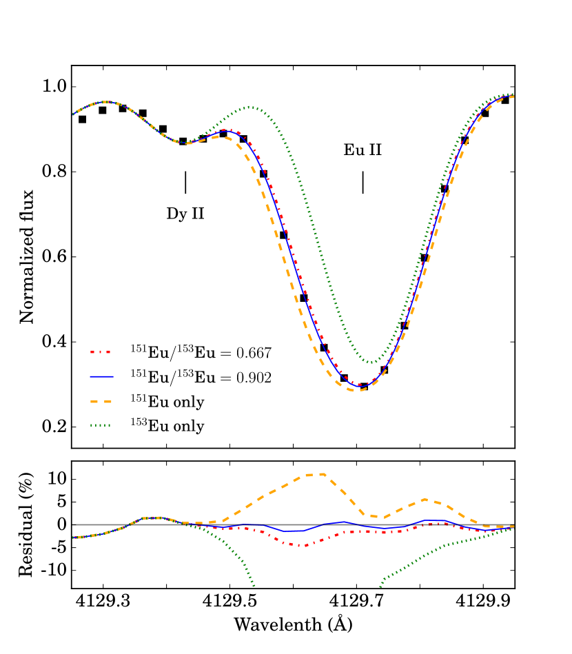
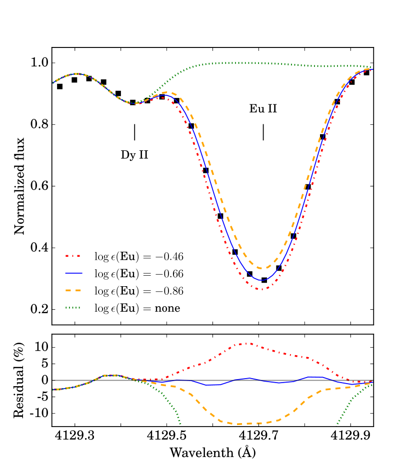
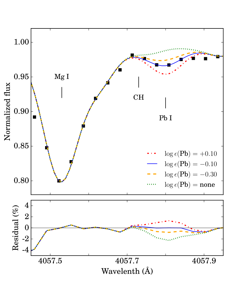
Figure 3: Observed spectra (squares) and synthesis (lines) for varying isotopic ratios of Eu II (left panel), and varying abundances of Eu II (middle panel), and Pb I (right panel).

Strontium, Yttrium, Zirconium

These three elements belong to the first r-process peak, and are often attributed to the weak r-process (Wanajo & Ishimaru, 2006). Their abundances are mostly determined from absorption lines in blue spectral regions, which can be affected by the presence of carbon features in CEMP stars, which does not apply to our current analysis. Siqueira Mello et al. (2014) have contrasted the behavior of these elements in r-I and r-II stars, finding that they are generally more enhanced in r-I stars, and suggested the possible existence of different nucleosynthesis pathways for these two sub-classes of r-process-enhanced stars.

The Sr $\lambda$4077 is saturated, but $\lambda$4215 could be successfully synthesized. The Sr line at $\lambda$4161 is a much weaker feature, and yields a slightly higher abundance than the $\lambda$4215 line. The left panel of Figure 2 shows the spectral synthesis of the Sr $\lambda$4215 line for three different abundances, and also for the absence of Sr.

The Y $\lambda$4398, $\lambda$4682, $\lambda$4883, and $\lambda$4900 lines are strong, well-isolated, and unsaturated. The feature at $\lambda$4982 is weak, but its abundance agrees well with the other four features.

Although most features of Zr are weak in the spectrum of RAVE J2038$-$0023 (catalog ), they are of sufficient strength to extract an abundance estimate from spectral synthesis; a total of six Zr features were used.

The final adopted abundances for the first peak elements are $[\mathrm{Sr}/\mathrm{Fe}]=+0.54$, $[\mathrm{Y}/\mathrm{Fe}]=+0.21$, and $[\mathrm{Zr}/\mathrm{Fe}]=+0.70$.

Barium, Lanthanum

These elements constitute the second r-process peak. The Ba lines on the blue spectral range were mostly saturated, so only the three lines at $\lambda$5853, $\lambda$6141, and $\lambda$6496 were used to determine the overall Ba abundance. Hyperfine splitting was accounted for in the spectral synthesis. The middle panel of Figure 2 shows the spectral synthesis of the Ba $\lambda$5853 line for three different abundances, and also for the absence of Ba. r-process isotopic fractions derived from solar abundances (Arlandini et al., 1999). These approximate the isotopic splitting of barium in RAVE J2038$-$0023 (catalog ) in order to produce a more accurate synthetic fit.

Six lines of La II were identified, and their derived abundances agree within 0.3 dex.

Final abundances of the second-peak elements are $[\mathrm{Ba}/\mathrm{Fe}]=+0.83$ and $[\mathrm{La}/\mathrm{Fe}]=+1.05$.

Cerium, Praseodymium, Neodymium, Samarium

A total of twelve Ce II lines were used to determine the abundance of cerium, more features than for any other neutron-capture element in RAVE J2038$-$0023 (catalog ). All Ce lines agree with the adopted abundance of $[\mathrm{Ce}/\mathrm{Fe}]=+0.98$ within 0.2 dex.

Seven strong praseodymium lines were used to find the Pr II abundance. There are two Pr II lines near the wings of the wide Ca II H feature at $\lambda$3968, but abundances derived from these lines still agree with the final abundance of $[\mathrm{Pr}/\mathrm{Fe}]=+1.30$. Similarly, the feature at $\lambda$4179 shows a blend with Nd II, but still agrees well with the adopted abundance.

There are many strong lines of neodymium, but several are blended with absorption features of other elements. In total, eleven Nd II features were used to determine the final abundance $[\mathrm{Nd}/\mathrm{Fe}]=+1.30$.

Five strong lines of samarium were used to determine the Sm II abundance. Although some lines showed a blend with other elements, all were taken into account, and the derived abundances agree with the final abundance $[\mathrm{Sm}/\mathrm{Fe}]=+1.42$ within 0.2 dex.

Europium

There are six europium lines with good agreement in their derived abundances, yielding an average $[\mathrm{Eu}/\mathrm{Fe}]=+1.64$. The middle panel of Figure 3 shows the spectral syntheses of the Eu $\lambda$4129 line for three different abundances, and also for the absence of Eu. Similarly to Ba, the strong lines of Eu are sensitive to hyperfine splitting between the isotopes ¹⁵¹Eu and ¹⁵³Eu. With high-resolution spectroscopy, this splitting has to be accounted for in spectral synthesis in order to fit the Eu II absorption features and measure the abundance. An isotopic ratio of ${}^{151}\text{Eu}/^{153}\text{Eu}=0.902$ (from solar r-process residuals; Arlandini et al., 1999) was used to approximate the effect of hyperfine splitting on the Eu II absorption features. For example, the left panel of Figure 3 shows the effect of varying the isotopic fraction ${}^{151}\text{Eu}/^{153}\text{Eu}$ at constant overall $\log\epsilon(\text{Eu})$ abundance. Clearly, only considering one isotope of Eu is not sufficient to describe the line shape. However the specific isotopic fraction cannot be measured this way. We only used it to calculate the Eu II abundance.

Gadolinium, Terbium, Dysprosium, Holmium, Erbium

Gadolinium features are often blended with neighboring lines or are located in the wings of strong hydrogen features, making their abundance measurements difficult. Still, all nine features agree within 0.2 dex of the adopted value of $[\mathrm{Gd}/\mathrm{Fe}]=+1.47$.

Five lines of terbium were used to estimate the Tb II abundance. The three Tb II lines at $\lambda$3702, $\lambda$3747, and $\lambda$3848 are blended with other features. However, two clean features at $\lambda$3874 and $\lambda$4002 yield similar abundances as those derived from the other three lines. The final adopted abundance is $[\mathrm{Tb}/\mathrm{Fe}]=+1.38$.

The dysprosium abundances derived from eight Dy II absorption features show a spread of 0.24 dex, yielding abundances around either $\log\epsilon\,(\mathrm{Dy})=-0.42$ or $\log\epsilon\,(\mathrm{Dy})=-0.25$. The final abundance is taken to be $[\mathrm{Dy}/\mathrm{Fe}]=+1.48$ by averaging all eight lines.

Three features of holmium were used to estimate its abundance. The Ho II lines at $\lambda$3810 and $\lambda$3890 in particular are blended with Fe features. However, since the estimates for the three lines agree within less than 0.1 dex, all were used for determining the final abundance, $[\mathrm{Ho}/\mathrm{Fe}]=+1.40$.

The abundance of erbium was estimated from seven Er II lines, all agreeing to within 0.2 dex of the adopted value, $[\mathrm{Er}/\mathrm{Fe}]=+1.60$.

Thulium, Ytterbium, Lutetium, Hafnium

Many Tm II features are found in the blue ($\lambda<4000$ Å) region of the spectrum. Five lines were used, and their estimates are in good agreement, yielding $[\mathrm{Tm}/\mathrm{Fe}]=+1.60$.

Only one strong Yb II line can be measured in the spectrum of RAVE J2038$-$0023 (catalog ). It neighbors a blended Fe-Ni feature to the blue. Regardless, the line at $\lambda$3694 was sufficiently strong to measure a ytterbium abundance with confidence ($[\mathrm{Yb}/\mathrm{Fe}]=+1.56$). The right panel of Figure 2 shows the spectral synthesis of the Yb $\lambda$3694 line for three different abundances, and also for the absence of Yb. Since the Yb II feature is well-described within a $\pm$0.2 dex variation from the adopted values, an uncertainty of $\pm$0.2 dex is assigned to the Yb II abundance.

Similarly, only two Lu II lines could be accurately fit with spectral synthesis. Both lines appear far in the blue, around 3500 Å, near the edge of the spectrum. The line at $\lambda$3472 appears blueward of a strong Ni I feature, so the line was fit by analyzing the asymmetry of the blended feature and fitting the blue wing. The line at $\lambda$3507 is blended with an iron feature, but its synthetic abundance agrees with that of the line at $\lambda$3472 Å, yielding a lutetium abundance of $[\mathrm{Lu}/\mathrm{Fe}]=+1.39$.

Four hafnium lines were used to etimate the final abundance of Hf II. The cleanest feature at $\lambda$3719 yielded the highest abundance, $\log\epsilon\,(\mathrm{Hf})=-0.5$. The two features at $\lambda$3793 and 3918 are uncertain, but agree with each other. The feature at $\lambda$4093 has the lowest derived abundance, $\log\epsilon\,(\mathrm{Hf})=-0.79$. The adopted hafnium abundance, from an average of all four lines, is $[\mathrm{Hf}/\mathrm{Fe}]=+1.40$.

Osmium and Iridium

Osmium and iridium represent the third r-process peak.

Three lines of Os I were used. The individual abundances calculated from these lines disagree (range of 0.45 dex), but it is still clear that the features are present. We obtain a final estimate of $[\mathrm{Os}/\mathrm{Fe}]=+1.60$ by averaging the three individual measurements.

Only the line at $\lambda$3800 could be used to estimate the iridium abundance. This feature appears in a crowded part of the spectrum, but the line is unblended, and could be well-fit by spectral synthesis. The adopted abundance of Ir I from this line is $[\mathrm{Ir}/\mathrm{Fe}]=+1.51$.

Lead

This third-peak element is typically largely produced by the s-process (Travaglio et al., 2001) in metal-poor stars. However, since RAVE J2038$-$0023 (catalog ) exhibits no s-process enhancement, and its neutron-capture elements likely result from only r-process events, the presence of Pb in RAVE J2038$-$0023 (catalog ) is not indicative of s-process enrichment. Rather, Wanajo et al. (2002) call attention to the importance of the third-peak element Pb for understanding the nature of the r-process, since it is mainly synthesized by the same $\alpha$-decay chains as Th and U.

Only the line at $\lambda$4057 was used to obtain the Pb I abundance. The right panel of Figure 3 shows the spectral synthesis of this line for three different abundances, and also for the absence of Pb. The final abundance is $[\mathrm{Pb}/\mathrm{Fe}]=+1.06$.

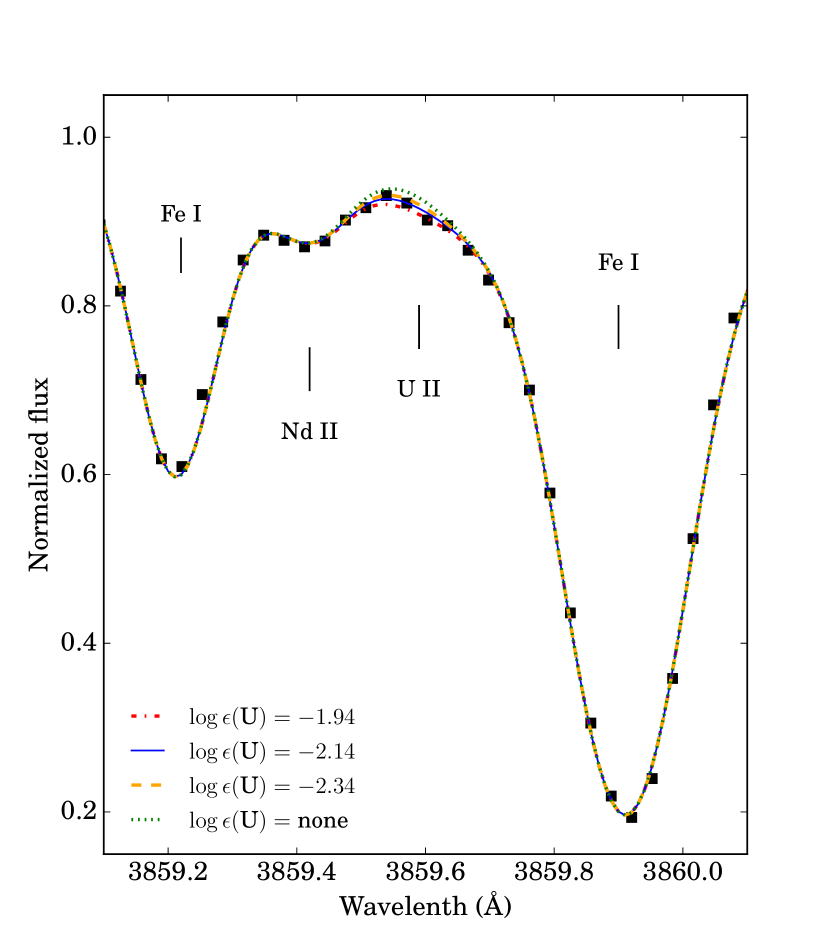
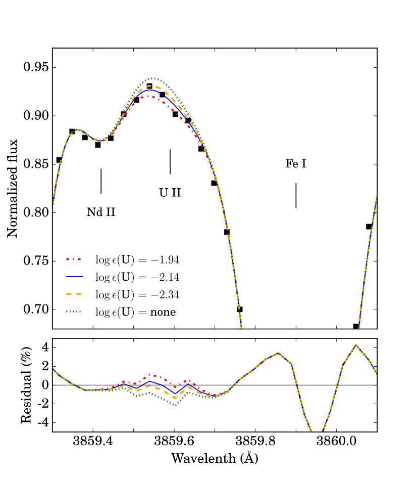
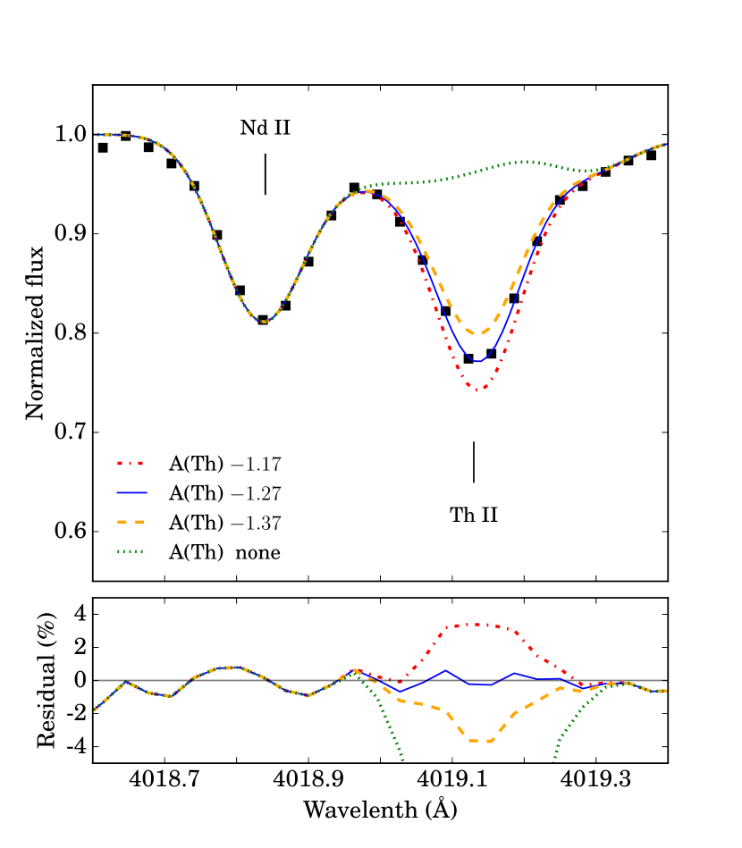
Figure 4: Observed spectra (squares) and synthesis (lines) of varying abundances of U II $\lambda$3859 (left and middle panels) and Th II $\lambda$4019 (right panel).

Thorium and Uranium

Thorium and uranium are radioactive actinides, and the heaviest observable elements in a stellar spectrum. These can only be synthesized in an r-process event. Furthermore, their presence allow the calculation of stellar ages (see Section 5.2).

Three lines of Th II were used to determine the final abundance. The feature at $\lambda$4019 (right panel of Figure 4) is the strongest, and blended with CH, Ni, and Pr features, which were accounted for in the synthesis. The other two Th features at $\lambda$4086 and $\lambda$4094 agree well with the adopted abundance, $[\mathrm{Th}/\mathrm{Fe}]=+1.65$.

Only one U II feature could be measured with accuracy. The $\lambda$3859 line appears at the far edge of a strong iron line, between a Nd II and a CN feature. After the abundances of neodymium and carbon are well-determined, the uranium feature was fit, and an abundance of $[\mathrm{U}/\mathrm{Fe}]=+1.31$ fits the data most accurately (see left and middle panels of Figure 4). From inspection of this figure, it is clear that a higher S/N spectrum would be useful to better constrain this determination.

5 Discussion

5.1 Heavy-Element Pattern for RAVE J2038$-$0023 (catalog )

The top panel of Figure 5 compares the measured neutron-capture elemental-abundance pattern with the scaled Solar System r-process pattern, normalized to the Eu abundance. The abundances of RAVE J2038$-$0023 (catalog ) agree well, and deviations from the Solar System r-process pattern (shown in the middle panel of Figure 5, normalized to Eu) indicate a suppression in the first r-process peak (elements Sr, Y, and Zr).

The first-peak elements are of particular interest, as they have been suggested by Siqueira Mello et al. (2014) and others to be associated with production by the weak, rather than the main, r-process (perhaps by neutrino-driven winds in core-collapse SNe - Arcones et al., 2007; Wanajo, 2007; Arcones & Thielemann, 2013). The slight under-abundance of the first-peak elements in RAVE J2038$-$0023 (catalog ) may support the argument for multiple r-process sites in which a weak r-process efficiently produces first-peak neutron-capture elements, but cannot robustly synthesize elements beyond the second peak. Furthermore, Siqueira Mello et al. (2014) have also presented evidence that the first-peak elements for moderately r-process-enhanced (r-I) stars generally exceed the levels found for r-II stars, and that this may indicate the operation of different nucleosynthesis pathways for these classes of stars.

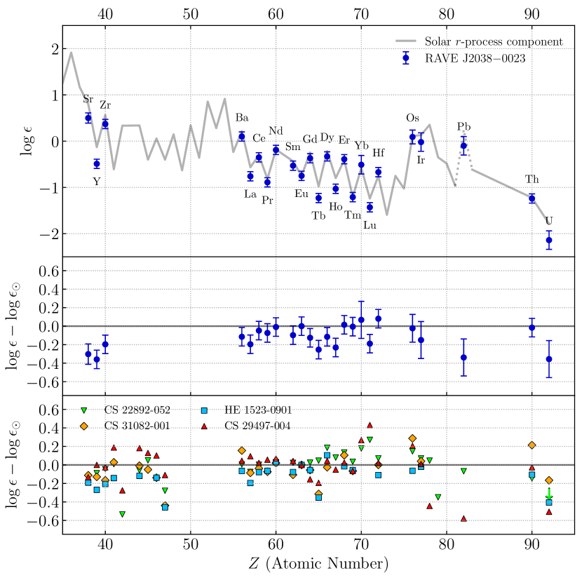
Figure 5: Top: Full neutron-capture elemental-abundance pattern for RAVE J2038$-$0023 (catalog ) compared with the Solar System r-process component (Arlandini et al., 1999), normalized to Eu. Middle: Difference between RAVE J2038$-$0023 (catalog ) abundances and the Solar System r-process component, normalized to Eu. Bottom: Same as middle panel, for the stars: CS 22892$-$052 (Sneden et al., 2008), CS 29497$-$004 (Hill et al., 2016), CS 31082$-$001 (Hill et al., 2002), and HE 1523$-$0901 (Frebel et al., 2007).

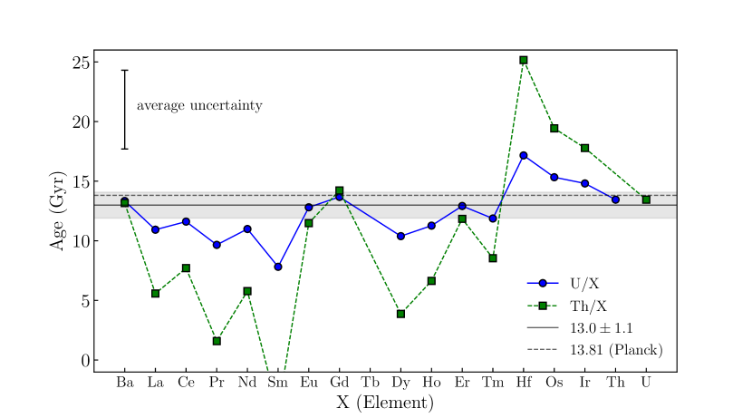
Figure 6: Radioactive-decay ages using PRs from Hill et al. (2016) for U/X (blue, solid, circles) and Th/X (green, dashed, squares). The solid horizontal line marks the mean age for RAVE J2038$-$0023 (catalog ) (see text for details), the shaded area represents its uncertainty, and the dashed horizontal line is the age of the Universe (Planck Collaboration et al., 2016). Also shown on the top left is a typical error bar for the individual age determinations. The production ratios and derived ages for individual chronometer pairs are listed Table 7.

Among the heaviest stable neutron-capture elements, it is worth noting that Pb is most discrepant from the scaled Solar System r-process pattern, for both RAVE J2038$-$0023 (catalog ) and CS 29407$−$004. This is due to the fact the the solar r-process pattern is derived from subtracting the s-process component of the total solar abundance pattern. The s-process at higher metallicity produces less Pb compared to other neutron-capture elements. This leads to an overestimated r-process Pb contribution when comparing a scaled solar r-process pattern and a low-metallicity star, as seen in Figure 5. For a more accurate comparison, a “low-metallicity” solar-process pattern would have to be derived. RAVE J2038$-$0023 (catalog ) has a $[\mathrm{Pb}/\mathrm{Eu}]$$=-0.68$, which is consistent with the production by the r-process at low metallicities (see Roederer et al. 2010 and Figure 15 of Placco et al. 2013).

The bottom panel of Figure 5 compares the residual abundances of four other r-II stars with reported measurements (and upper limits) of U. Although there appears to be some small differences in the derived abundances between the U stars, their patterns largely agree within the uncertainties. Even among the r-II stars, there appears to be some real scatter in the first-peak elements Sr, Y, and Zr, with RAVE J2038$-$0023 (catalog ) being generally lower than the other U stars. For Th and U, RAVE J2038$-$0023 (catalog ) appears commensurate with CS 29407$-$004 and HE 1523$-$0901, which are not actinide-boost stars, and all three are lower than the one U star known to exhibit an actinide boost, CS 31082$-$001. The actinide boost has also been recognized in HE 1219$-$0312, another r-II star with measurable Th, but lacking a detectable uranium feature (Barklem et al., 2005), given its faint magnitude. The over-abundance of the actinides in some r-II stars might suggest different r-process formation scenarios involving one or multiple r-process from sources, such as a high-entropy wind from SNII and the ejecta from neutron star mergers (see Mashonkina et al., 2010, for further details).

5.2 Age Determinations

The presence of radioactive elements Th and U in RAVE J2038$-$0023 (catalog ) allows for the determination of the star’s age (or more correctly, the time that has passed since the production of these elements) through radioactive decay dating. Radioactive decay ages are estimated by measuring the relative abundances of long-lived radioactive elements (i.e., ²³²Th: $t_{1/2}=14.0$ Gyr, and ²³⁸U: $t_{1/2}=4.5$ Gyr) to stable elements (i.e., the ratios Th/X and U/X, where X is a stable element) or the ratio between the radioactive elements themselves (Th/U).

To make use of radioactive decay dating, a set of initial production ratios (PRs: $\text{Th/X}_{0}$, $\text{U/X}_{0}$, and $\text{Th/U}_{0}$) must be estimated. For the present work, we use PRs from (i) the r-process waiting-point calculations of Schatz et al. (2002) and from (ii) Hill et al. (2016) based on the high-entropy wind model of Farouqi et al. (2010). With PRs in hand, the ages $t$ are calculated as follows:

$$t= 46.67\mbox{ Gyr }\left[\log\epsilon\left(\text{Th/X}\right)_{0}-\log\epsilon\left(\text{Th/X}\right)_{\text{obs}}\right],$$ (1)

$$t= 14.84\mbox{ Gyr }\left[\log\epsilon\left(\text{U/X}\right)_{0}-\log\epsilon\left(\text{U/X}\right)_{\text{obs}}\right],$$ (2)

and

$$t= 21.80\mbox{ Gyr }\left[\log\epsilon\left(\text{U/Th}\right)_{0}-\log\epsilon\left(\text{U/Th}\right)_{\text{obs}}\right],$$ (3)

where $\log\epsilon\left(\text{Th/X}\right)_{0}$ is the initial PR corresponding to element formation at $t=0$, and $\log\epsilon\left(\text{Th/X}\right)_{\text{obs}}$ is the observed ratio after the radioactive elements Th and U have decayed for a time $t$. The half-lives of Th and U are contained in the constant. Table 7 lists the PRs used in the above equations and the ages derived from these abundance ratios. The calculated U/X and Th/X ages using the PRs from Hill et al. (2016) are shown in Figure 6. The solid horizontal line marks the mean age for RAVE J2038$-$0023 (catalog ) (see details below), and the dashed horizontal line is the age of the Universe, determined by the Planck mission (Planck Collaboration et al., 2016).

Arithmetic means were taken for all four sets of ages: U/X and Th/X, each using the two different sets of PRs described above. All U/X and Th/X ages agree within $2\sigma$ of their arithmetic means except for ages calculated from Hf ratios in the Schatz et al. (2002) model (see Table 7). The small uncertainty on the Hf abundance suggests that the discrepancy between X/Hf and other ages is driven by the predicted production ratio for this chronometer pair by both r-process models considered above. The same inconsistency of X/Hf ages was also noticed by Hill et al. (2016) in their analysis of the U star CS 29497$-$004.

The uncertainties in Table 7 reflect only the propagated error from the abundance measurement uncertainty; systematic errors from the model atmosphere parameters as well as uncertainties from the r-process models considered here were not included. Since only one U II feature could be measured, the uncertainty associated with the U II abundance is set to 0.2 dex. The syntheses in Figure 4 show the best-fit abundance as well as $\pm 0.2$ dex from the best fit. Since the feature is well-described within these limits, an uncertainty of 0.2 dex is suitable for the uranium abundance.

Although the uncertainty on the uranium abundance is larger than that of thorium (0.2 and 0.04 dex, respectively), the individual U/X ages vary much less than the Th/X ages. This apparent contradiction results primarily from the longer half-life of ²³²Th (and therefore the larger constant in Equation 1), causing Th/X ages to be much more sensitive to variations on the measured Th/X abundance ratios. On the other hand, U/X ages—albeit carrying large uncertainties—agree with the expected ages of VMP/EMP stars.

From Figure 6, it is interesting to note that the ages calculated for Ba, Eu, Gd, and Er, using both Th/X and U/X ratios, agree with each other and with the Th/U age of $13.4$ Gyr, using the PRs of Hill et al. (2016). The mean age for Th/X, using Ba, Eu, Gd, and Er, is $12.7\pm 1.6$ Gyr, while the mean age for U/X with the same four elements is $13.2\pm 1.5$ Gyr. The fact that these elements present a much smaller scatter between the Th/X and U/X ratios suggests that these are more likely to represent a realistic age for RAVE J2038$-$0023 (catalog ). Then, by averaging Th/X and U/X ratios for Ba, Eu, Gd, and Er, and Th/U (with PRs from Hill et al., 2016), we adopt an age of $13.0\pm 1.1$ Gyr for RAVE J2038$-$0023 (catalog ).

6 Conclusions

We have presented results for the first r-II star discovered from the RAVE survey, RAVE J2038$-$0023 (catalog ), and only the fourth r-II star with measured Th and U. This star was first identified as a metal-poor candidate from the RAVE DR4, and then followed-up with medium- and high-resolution spectroscopy with the Mayall and Magellan telescopes, respectively.

A detailed high-resolution abundance analysis reveals that the chemical abundance pattern of RAVE J2038$-$0023 (catalog ) nearly duplicates the scaled Solar System r-process pattern, similar to the other three known U stars and other r-II stars. With measured abundances for the actinides thorium and uranium, we were able to determine radioactive-decay ages for RAVE J2038$-$0023 (catalog ) from Th/X and U/X abundance ratios, using initial production ratios from an r-process high-entropy wind model. The estimated age for RAVE J2038$-$0023 (catalog ) (13.0$\pm$1.1 Gyr) is consistent with expectations for the epoch in which VMP/EMP stars formed. We note that the yields of a neutron star merger r-process may differ from the standard scenarios considered here. We plan to update our age estimates as realistic yields from these events become available.

We are presently extending our effort to identify large numbers of r-II (and r-I) stars, based on medium-resolution spectroscopy of a large number ($\sim 2000-2500$) of bright targets with [Fe/H] $<-2.0$ from a number of sources, in addition to RAVE. High-resolution spectroscopic follow-up of these targets, already underway, should identify on the order of 75 new r-II (and 350 new r-I) stars. This would provide a sufficiently large sample to carry out detailed tests of the likely astrophysical site(s) of the production of the r-process elements in the early Galaxy, and tests of the association of r-II (and r-I) stars in the field with particular environments, such as the ultra-faint and canonical dwarf galaxies in which similar stars have been previously identified (see Hansen et al., 2017, and references therein).

Table 3: Equivalent-Width Measurements for RAVE J2038$-$0023 (catalog )

Ion	$\lambda$	$\chi$	$\log\,gf$	$W$	$\log\epsilon$ (X)
	(Å)	(eV)		(mÅ)
Na I	5889.950	0.00	0.108	171.69	3.72
Mg I	3829.355	2.71	$-$0.208	153.47	5.08
Mg I	3832.304	2.71	0.270	192.31	4.97
Mg I	3986.753	4.35	$-$1.030	21.60	5.10
Mg I	4057.505	4.35	$-$0.890	23.68	5.00
Mg I	4167.271	4.35	$-$0.710	35.18	5.05
Mg I	4571.096	0.00	$-$5.688	62.43	5.13
Mg I	4702.990	4.33	$-$0.380	60.66	5.02
Mg I	5172.684	2.71	$-$0.450	182.51	5.04
Mg I	5183.604	2.72	$-$0.239	208.96	5.08
Mg I	5528.405	4.34	$-$0.498	60.46	5.06
Al I	3961.520	0.01	$-$0.340	122.10	3.09
Si I	3905.523	1.91	$-$1.092	192.86	5.17
Si I	4102.936	1.91	$-$3.140	74.50	5.21
Ca I	4226.730	0.00	0.244	187.14	3.47
Ca I	4283.010	1.89	$-$0.224	36.01	3.51
Ca I	4318.650	1.89	$-$0.210	39.49	3.56
Ca I	4425.440	1.88	$-$0.358	30.44	3.50
Ca I	4455.890	1.90	$-$0.530	24.40	3.55
Ca I	5588.760	2.52	0.210	34.30	3.64
Ca I	5594.468	2.52	0.097	31.59	3.69
Ca I	5598.487	2.52	$-$0.087	20.71	3.63
Ca I	5857.450	2.93	0.230	15.88	3.65
Ca I	6102.720	1.88	$-$0.790	23.66	3.61
Ca I	6122.220	1.89	$-$0.315	52.46	3.67
Ca I	6162.170	1.90	$-$0.089	63.69	3.63
Ca I	6439.070	2.52	0.470	48.99	3.58
Sc II	4314.083	0.62	$-$0.100	87.86	0.27
Sc II	4324.998	0.59	$-$0.440	70.00	0.18
Sc II	4400.389	0.61	$-$0.540	63.60	0.17
Sc II	4415.544	0.59	$-$0.670	59.26	0.19
Sc II	5031.010	1.36	$-$0.400	28.79	0.23
Sc II	5526.785	1.77	0.020	24.65	0.17
Sc II	5657.907	1.51	$-$0.600	16.86	0.26
Sc II	6604.578	1.36	$-$1.310	5.94	0.21
Ti I	3989.760	0.02	$-$0.062	60.52	2.17
Ti I	3998.640	0.05	0.010	59.89	2.12
Ti I	4533.249	0.85	0.532	44.80	2.12
Ti I	4534.780	0.84	0.336	32.51	2.07
Ti I	4535.567	0.83	0.120	24.87	2.12
Ti I	4656.470	0.00	$-$1.289	12.26	2.12
Ti I	4681.910	0.05	$-$1.015	18.01	2.09
Ti I	4981.730	0.84	0.560	51.75	2.12
Ti I	4991.070	0.84	0.436	43.39	2.10
Ti I	4999.500	0.83	0.306	40.33	2.16
Ti I	5039.960	0.02	$-$1.130	17.85	2.12
Ti I	5210.390	0.05	$-$0.828	29.14	2.11
Ti II	3813.394	0.61	$-$2.020	59.03	2.19
Ti II	4025.120	0.61	$-$1.980	65.52	2.18
Ti II	4053.829	1.89	$-$1.210	26.32	2.19
Ti II	4161.527	1.08	$-$2.160	28.86	2.18
Ti II	4290.219	1.16	$-$0.930	84.74	2.11
Ti II	4300.049	1.18	$-$0.490	102.20	2.12
Ti II	4330.723	1.18	$-$2.060	30.50	2.20
Ti II	4337.914	1.08	$-$0.960	89.61	2.14
Ti II	4394.059	1.22	$-$1.780	44.15	2.21
Ti II	4395.031	1.08	$-$0.540	109.36	2.17
Ti II	4395.839	1.24	$-$1.930	31.59	2.15
Ti II	4399.765	1.24	$-$1.190	70.75	2.13
Ti II	4417.714	1.17	$-$1.190	74.65	2.12
Ti II	4418.331	1.24	$-$1.970	29.85	2.15
Ti II	4443.801	1.08	$-$0.720	102.84	2.15
Ti II	4444.554	1.12	$-$2.240	25.48	2.18
Ti II	4450.482	1.08	$-$1.520	62.62	2.09
Ti II	4464.448	1.16	$-$1.810	45.36	2.17
Ti II	4468.517	1.13	$-$0.600	107.79	2.20
Ti II	4470.853	1.17	$-$2.020	35.00	2.21
Ti II	4501.270	1.12	$-$0.770	98.75	2.13
Ti II	4533.960	1.24	$-$0.530	101.99	2.10
Ti II	4563.770	1.22	$-$0.960	89.70	2.21
Ti II	4571.971	1.57	$-$0.320	96.06	2.15
Ti II	4589.915	1.24	$-$1.790	43.05	2.19
Ti II	4657.200	1.24	$-$2.240	19.14	2.13
Ti II	4708.662	1.24	$-$2.340	18.37	2.20
Ti II	4779.979	2.05	$-$1.370	17.26	2.18
Ti II	4805.089	2.06	$-$1.100	27.86	2.18
Ti II	5129.156	1.89	$-$1.240	31.65	2.15
Ti II	5185.902	1.89	$-$1.490	22.26	2.19
Ti II	5336.786	1.58	$-$1.590	36.34	2.18
Ti II	5381.021	1.57	$-$1.920	21.86	2.19
Ti II	5418.768	1.58	$-$2.000	17.70	2.17
V II	3951.960	1.48	$-$0.784	30.75	1.28
V II	4035.622	1.79	$-$0.767	18.53	1.33
Cr I	3578.680	0.00	0.420	97.67	2.38
Cr I	4254.332	0.00	$-$0.114	108.51	2.45
Cr I	4274.800	0.00	$-$0.220	105.31	2.46
Cr I	4545.950	0.94	$-$1.370	8.53	2.38
Cr I	4600.752	1.00	$-$1.260	11.89	2.50
Cr I	4616.137	0.98	$-$1.190	13.15	2.45
Cr I	4626.188	0.97	$-$1.320	10.36	2.45
Cr I	4646.150	1.03	$-$0.740	27.92	2.46
Cr I	4651.280	0.98	$-$1.460	7.80	2.46
Cr I	4652.158	1.00	$-$1.030	15.28	2.39
Cr I	5206.040	0.94	0.020	82.59	2.49
Cr I	5296.690	0.98	$-$1.360	10.83	2.44
Cr I	5298.280	0.98	$-$1.140	17.81	2.47
Cr I	5345.800	1.00	$-$0.950	24.19	2.46
Cr I	5348.310	1.00	$-$1.210	13.40	2.42
Cr I	5409.770	1.03	$-$0.670	38.95	2.50
Mn I	4030.753	0.00	$-$0.480	98.98	1.98
Mn I	4033.062	0.00	$-$0.618	95.43	2.01
Mn I	4034.483	0.00	$-$0.811	89.39	2.03
Mn I	4041.357	2.11	0.285	23.28	2.02
Mn I	4754.048	2.28	$-$0.086	9.47	2.00
Mn I	4783.432	2.30	0.042	11.95	2.00
Mn I	4823.528	2.32	0.144	14.06	2.00
Fe I	3608.859	1.01	$-$0.090	149.26	4.48
Fe I	3767.192	1.01	$-$0.390	145.10	4.48
Fe I	3787.880	1.01	$-$0.838	125.95	4.60
Fe I	3815.840	1.48	0.237	155.99	4.49
Fe I	3840.438	0.99	$-$0.497	157.67	4.61
Fe I	3841.048	1.61	$-$0.044	132.50	4.58
Fe I	3845.169	2.42	$-$1.390	27.87	4.41
Fe I	3846.800	3.25	$-$0.020	52.97	4.60
Fe I	3849.967	1.01	$-$0.863	118.69	4.38
Fe I	3863.741	2.69	$-$1.430	18.18	4.51
Fe I	3865.523	1.01	$-$0.950	119.79	4.48
Fe I	3867.216	3.02	$-$0.450	42.76	4.51
Fe I	3885.510	2.42	$-$1.090	34.42	4.24
Fe I	3886.282	0.05	$-$1.080	179.35	4.55
Fe I	3895.656	0.11	$-$1.668	136.17	4.56
Fe I	3902.946	1.56	$-$0.442	119.56	4.62
Fe I	3920.258	0.12	$-$1.734	135.98	4.60
Fe I	3977.741	2.20	$-$1.120	66.77	4.68
Fe I	4001.661	2.18	$-$1.900	20.70	4.40
Fe I	4005.242	1.56	$-$0.583	114.09	4.56
Fe I	4007.272	2.76	$-$1.280	22.20	4.52
Fe I	4032.627	1.49	$-$2.380	36.85	4.40
Fe I	4044.609	2.83	$-$1.220	21.78	4.52
Fe I	4045.812	1.49	0.284	176.21	4.56
Fe I	4058.217	3.21	$-$1.110	12.93	4.58
Fe I	4062.441	2.85	$-$0.860	37.19	4.53
Fe I	4063.594	1.56	0.062	148.94	4.53
Fe I	4067.978	3.21	$-$0.470	31.54	4.45
Fe I	4070.769	3.24	$-$0.790	18.86	4.50
Fe I	4071.738	1.61	$-$0.008	146.48	4.62
Fe I	4073.763	3.27	$-$0.900	16.39	4.56
Fe I	4098.176	3.24	$-$0.880	18.97	4.58
Fe I	4114.445	2.83	$-$1.303	20.31	4.54
Fe I	4120.207	2.99	$-$1.270	16.12	4.58
Fe I	4121.802	2.83	$-$1.450	15.30	4.54
Fe I	4132.899	2.85	$-$1.010	24.62	4.38
Fe I	4134.678	2.83	$-$0.649	45.52	4.44
Fe I	4136.998	3.42	$-$0.450	24.65	4.51
Fe I	4139.927	0.99	$-$3.629	20.16	4.63
Fe I	4143.414	3.05	$-$0.200	52.61	4.40
Fe I	4143.868	1.56	$-$0.511	123.11	4.59
Fe I	4153.899	3.40	$-$0.320	26.19	4.39
Fe I	4154.498	2.83	$-$0.688	42.67	4.42
Fe I	4154.805	3.37	$-$0.400	25.64	4.42
Fe I	4156.799	2.83	$-$0.808	35.35	4.39
Fe I	4157.780	3.42	$-$0.403	23.58	4.42
Fe I	4158.793	3.43	$-$0.670	17.00	4.52
Fe I	4174.913	0.91	$-$2.938	54.65	4.55
Fe I	4181.755	2.83	$-$0.371	62.65	4.50
Fe I	4182.382	3.02	$-$1.180	15.52	4.49
Fe I	4184.892	2.83	$-$0.869	42.12	4.58
Fe I	4187.039	2.45	$-$0.514	81.84	4.61
Fe I	4187.795	2.42	$-$0.510	81.71	4.57
Fe I	4191.430	2.47	$-$0.666	65.71	4.42
Fe I	4195.329	3.33	$-$0.492	24.83	4.43
Fe I	4199.095	3.05	0.156	74.15	4.50
Fe I	4202.029	1.49	$-$0.689	115.75	4.48
Fe I	4217.545	3.43	$-$0.484	22.96	4.49
Fe I	4222.213	2.45	$-$0.914	59.17	4.48
Fe I	4227.427	3.33	0.266	65.76	4.52
Fe I	4233.603	2.48	$-$0.579	73.99	4.50
Fe I	4238.810	3.40	$-$0.233	35.90	4.49
Fe I	4250.119	2.47	$-$0.380	83.66	4.51
Fe I	4250.787	1.56	$-$0.713	119.93	4.65
Fe I	4260.474	2.40	0.077	109.20	4.56
Fe I	4271.154	2.45	$-$0.337	91.65	4.62
Fe I	4271.760	1.49	$-$0.173	145.53	4.51
Fe I	4325.762	1.61	0.006	149.85	4.52
Fe I	4337.046	1.56	$-$1.695	75.15	4.48
Fe I	4352.735	2.22	$-$1.290	56.59	4.49
Fe I	4375.930	0.00	$-$3.005	109.99	4.70
Fe I	4383.545	1.48	0.200	177.72	4.49
Fe I	4388.407	3.60	$-$0.681	11.49	4.49
Fe I	4404.750	1.56	$-$0.147	155.74	4.64
Fe I	4407.709	2.18	$-$1.970	34.42	4.68
Fe I	4415.122	1.61	$-$0.621	121.77	4.55
Fe I	4427.310	0.05	$-$2.924	109.71	4.65
Fe I	4430.614	2.22	$-$1.659	40.74	4.54
Fe I	4442.339	2.20	$-$1.228	67.20	4.58
Fe I	4443.194	2.86	$-$1.043	27.12	4.42
Fe I	4447.717	2.22	$-$1.339	55.97	4.50
Fe I	4454.381	2.83	$-$1.300	25.98	4.62
Fe I	4459.118	2.18	$-$1.279	66.05	4.58
Fe I	4461.653	0.09	$-$3.194	100.87	4.71
Fe I	4476.019	2.85	$-$0.820	46.66	4.57
Fe I	4484.220	3.60	$-$0.860	10.23	4.60
Fe I	4489.739	0.12	$-$3.899	66.33	4.65
Fe I	4494.563	2.20	$-$1.143	70.78	4.55
Fe I	4531.148	1.48	$-$2.101	69.10	4.58
Fe I	4592.651	1.56	$-$2.462	52.22	4.71
Fe I	4602.941	1.49	$-$2.208	66.23	4.63
Fe I	4630.120	2.28	$-$2.587	8.70	4.65
Fe I	4632.912	1.61	$-$2.913	23.49	4.66
Fe I	4647.434	2.95	$-$1.351	20.30	4.64
Fe I	4678.846	3.60	$-$0.830	12.03	4.62
Fe I	4691.411	2.99	$-$1.520	13.24	4.63
Fe I	4707.274	3.24	$-$1.080	17.19	4.62
Fe I	4710.283	3.02	$-$1.610	9.42	4.59
Fe I	4733.591	1.49	$-$2.988	26.27	4.64
Fe I	4736.772	3.21	$-$0.752	31.04	4.59
Fe I	4786.806	3.00	$-$1.606	10.75	4.62
Fe I	4859.741	2.88	$-$0.760	53.00	4.58
Fe I	4871.318	2.87	$-$0.362	72.14	4.52
Fe I	4872.137	2.88	$-$0.567	54.38	4.42
Fe I	4890.755	2.88	$-$0.394	72.42	4.56
Fe I	4891.492	2.85	$-$0.111	85.16	4.50
Fe I	4903.310	2.88	$-$0.926	37.13	4.46
Fe I	4918.994	2.85	$-$0.342	73.33	4.48
Fe I	4924.770	2.28	$-$2.114	24.33	4.65
Fe I	4938.814	2.88	$-$1.077	30.63	4.48
Fe I	4939.687	0.86	$-$3.252	57.14	4.65
Fe I	4946.388	3.37	$-$1.170	11.59	4.64
Fe I	4966.089	3.33	$-$0.871	20.26	4.58
Fe I	4994.130	0.92	$-$2.969	69.41	4.65
Fe I	5001.870	3.88	0.050	30.48	4.55
Fe I	5012.068	0.86	$-$2.642	96.10	4.79
Fe I	5041.072	0.96	$-$3.090	60.04	4.64
Fe I	5041.756	1.49	$-$2.200	75.76	4.70
Fe I	5049.820	2.28	$-$1.355	59.37	4.52
Fe I	5051.634	0.92	$-$2.764	85.91	4.75
Fe I	5068.766	2.94	$-$1.041	29.33	4.47
Fe I	5074.749	4.22	$-$0.200	10.07	4.60
Fe I	5079.224	2.20	$-$2.105	24.55	4.53
Fe I	5079.740	0.99	$-$3.245	57.51	4.79
Fe I	5083.339	0.96	$-$2.842	73.53	4.63
Fe I	5098.697	2.18	$-$2.030	43.97	4.81
Fe I	5110.413	0.00	$-$3.760	95.98	4.79
Fe I	5127.360	0.92	$-$3.249	56.69	4.68
Fe I	5131.468	2.22	$-$2.515	12.58	4.62
Fe I	5133.689	4.18	0.140	18.84	4.52
Fe I	5142.929	0.96	$-$3.080	66.14	4.73
Fe I	5150.839	0.99	$-$3.037	59.45	4.60
Fe I	5151.911	1.01	$-$3.321	51.73	4.78
Fe I	5166.282	0.00	$-$4.123	78.79	4.79
Fe I	5171.596	1.49	$-$1.721	96.70	4.62
Fe I	5191.455	3.04	$-$0.551	56.08	4.57
Fe I	5192.344	3.00	$-$0.421	56.61	4.40
Fe I	5194.942	1.56	$-$2.021	83.02	4.72
Fe I	5198.711	2.22	$-$2.091	24.66	4.53
Fe I	5202.336	2.18	$-$1.871	42.80	4.62
Fe I	5216.274	1.61	$-$2.082	66.28	4.52
Fe I	5225.526	0.11	$-$4.755	33.12	4.76
Fe I	5232.940	2.94	$-$0.057	82.71	4.43
Fe I	5242.491	3.63	$-$0.967	8.44	4.56
Fe I	5247.050	0.09	$-$4.946	28.26	4.84
Fe I	5250.210	0.12	$-$4.938	21.48	4.71
Fe I	5250.646	2.20	$-$2.180	34.67	4.80
Fe I	5254.956	0.11	$-$4.764	37.38	4.85
Fe I	5266.555	3.00	$-$0.385	65.34	4.51
Fe I	5269.537	0.86	$-$1.333	159.43	4.76
Fe I	5281.790	3.04	$-$0.833	41.05	4.58
Fe I	5283.621	3.24	$-$0.524	41.32	4.52
Fe I	5302.300	3.28	$-$0.720	30.24	4.56
Fe I	5307.361	1.61	$-$2.912	25.00	4.60
Fe I	5324.179	3.21	$-$0.103	61.72	4.40
Fe I	5328.039	0.92	$-$1.466	152.54	4.82
Fe I	5328.531	1.56	$-$1.850	92.61	4.71
Fe I	5332.900	1.55	$-$2.776	31.82	4.54
Fe I	5339.930	3.27	$-$0.720	30.56	4.55
Fe I	5364.871	4.45	0.228	12.87	4.54
Fe I	5365.400	3.56	$-$1.020	11.05	4.65
Fe I	5371.489	0.96	$-$1.644	148.24	4.95
Fe I	5383.369	4.31	0.645	35.53	4.52
Fe I	5393.168	3.24	$-$0.910	32.33	4.73
Fe I	5397.128	0.92	$-$1.982	129.30	4.83
Fe I	5405.775	0.99	$-$1.852	136.75	4.95
Fe I	5415.199	4.39	0.643	35.76	4.63
Fe I	5424.068	4.32	0.520	33.18	4.61
Fe I	5429.696	0.96	$-$1.881	132.11	4.84
Fe I	5434.524	1.01	$-$2.126	116.05	4.79
Fe I	5446.917	0.99	$-$1.910	132.28	4.90
Fe I	5455.609	1.01	$-$2.090	123.53	4.90
Fe I	5497.516	1.01	$-$2.825	80.46	4.74
Fe I	5501.465	0.96	$-$3.046	75.60	4.80
Fe I	5506.779	0.99	$-$2.789	81.84	4.69
Fe I	5569.618	3.42	$-$0.540	29.34	4.50
Fe I	5572.842	3.40	$-$0.275	45.50	4.52
Fe I	5576.088	3.43	$-$1.000	14.19	4.58
Fe I	5586.756	3.37	$-$0.144	55.13	4.50
Fe I	5615.644	3.33	0.050	70.83	4.53
Fe I	5658.816	3.40	$-$0.793	22.66	4.58
Fe I	5662.516	4.18	$-$0.573	6.78	4.69
Fe I	5701.544	2.56	$-$2.143	12.34	4.59
Fe I	6065.481	2.61	$-$1.410	37.90	4.51
Fe I	6136.615	2.45	$-$1.410	52.64	4.55
Fe I	6137.691	2.59	$-$1.346	41.54	4.49
Fe I	6191.558	2.43	$-$1.416	56.39	4.59
Fe I	6219.280	2.20	$-$2.448	21.40	4.70
Fe I	6230.723	2.56	$-$1.276	51.97	4.54
Fe I	6252.555	2.40	$-$1.687	42.20	4.59
Fe I	6254.257	2.28	$-$2.443	24.66	4.86
Fe I	6265.134	2.18	$-$2.540	24.31	4.83
Fe I	6335.330	2.20	$-$2.180	32.04	4.65
Fe I	6393.601	2.43	$-$1.576	46.87	4.59
Fe I	6411.649	3.65	$-$0.595	21.03	4.58
Fe I	6421.350	2.28	$-$2.014	33.60	4.60
Fe I	6430.846	2.18	$-$1.946	43.03	4.58
Fe I	6494.980	2.40	$-$1.239	76.18	4.67
Fe I	6592.912	2.73	$-$1.473	30.35	4.54
Fe I	6663.440	2.42	$-$2.479	11.55	4.66
Fe I	6677.986	2.69	$-$1.418	37.18	4.56
Fe I	6978.850	2.48	$-$2.452	10.98	4.66
Fe II	4489.185	2.83	$-$2.970	14.64	4.59
Fe II	4491.410	2.86	$-$2.710	19.12	4.51
Fe II	4515.340	2.84	$-$2.600	28.14	4.59
Fe II	4520.224	2.81	$-$2.600	31.25	4.62
Fe II	4541.523	2.86	$-$3.050	10.75	4.54
Fe II	4555.890	2.83	$-$2.400	35.36	4.52
Fe II	4576.340	2.84	$-$2.950	16.37	4.63
Fe II	4583.840	2.81	$-$1.930	60.14	4.47
Fe II	4923.930	2.89	$-$1.320	93.25	4.53
Fe II	5197.580	3.23	$-$2.220	26.54	4.56
Fe II	5234.630	3.22	$-$2.180	32.27	4.62
Fe II	5276.000	3.20	$-$2.010	42.66	4.61
Fe II	5284.080	2.89	$-$3.190	10.78	4.64
Co I	3842.047	0.92	$-$0.770	47.49	2.23
Co I	3845.468	0.92	0.010	81.12	2.30
Co I	3881.869	0.58	$-$1.130	52.85	2.27
Co I	3995.306	0.92	$-$0.220	73.10	2.19
Co I	4118.767	1.05	$-$0.490	60.17	2.26
Co I	4121.318	0.92	$-$0.320	74.45	2.25
Ni I	3500.850	0.17	$-$1.294	88.63	3.30
Ni I	3524.540	0.03	0.007	171.36	3.21
Ni I	3566.370	0.42	$-$0.251	116.06	3.20
Ni I	3597.710	0.21	$-$1.115	99.47	3.31
Ni I	3807.140	0.42	$-$1.220	97.22	3.29
Ni I	3858.301	0.42	$-$0.951	108.26	3.25
Ni I	4648.659	3.42	$-$0.160	8.30	3.27
Ni I	4714.421	3.38	0.230	17.96	3.21
Ni I	4904.410	3.54	$-$0.170	6.04	3.24
Ni I	4980.161	3.61	$-$0.110	6.33	3.28
Ni I	5080.523	3.65	0.130	7.95	3.19
Ni I	5084.080	3.68	0.030	5.35	3.14
Ni I	5476.900	1.83	$-$0.890	60.32	3.18
Ni I	5754.675	1.94	$-$2.330	3.10	3.09
Ni I	6108.121	1.68	$-$2.450	5.53	3.12
Zn I	4722.150	4.03	$-$0.390	7.68	1.75
Zn I	4810.528	4.08	$-$0.137	10.51	1.70

Table 4: Individual Abundance Measurements of Neutron-Capture Elements for RAVE J2038$-$0023 (catalog )

Ion	$\lambda$	$\chi$	$\log\,gf$	$\log\epsilon$ (X)
	(Å)	(eV)
Sr II	4161.792	2.94	$-$0.502	0.56
Sr II	4215.519	0.00	$-$0.170	0.43
Y II	3747.556	0.10	$-$0.910	$-$0.34
Y II	4398.013	0.13	$-$1.000	$-$0.49
Y II	4682.324	0.41	$-$1.510	$-$0.38
Y II	4883.684	1.08	0.070	$-$0.52
Y II	4900.120	1.03	$-$0.090	$-$0.72
Zr II	3573.055	0.32	$-$1.041	0.42
Zr II	3836.761	0.56	$-$0.120	0.38
Zr II	3991.127	0.76	$-$0.310	0.28
Zr II	3998.954	0.56	$-$0.520	0.36
Zr II	4317.299	0.71	$-$1.450	0.38
Zr II	4050.316	0.71	$-$1.060	0.38
Ba II	5853.675	0.60	$-$1.010	$-$0.03
Ba II	6141.713	0.70	$-$0.077	0.08
Ba II	6496.898	0.60	$-$0.380	0.25
La II	3794.774	0.24	0.140	$-$0.60
La II	3988.515	0.40	0.170	$-$0.80
La II	3995.745	0.17	$-$0.100	$-$0.70
La II	4086.709	0.00	0.230	$-$0.70
La II	4123.218	0.32	0.110	$-$0.85
La II	4429.905	0.24	$-$1.490	$-$0.90
Ce II	3940.330	0.32	$-$0.270	$-$0.35
Ce II	3942.151	0.000	$-$0.22	$-$0.37
Ce II	3999.237	0.30	0.090	$-$0.23
Ce II	4014.897	0.53	0.140	$-$0.48
Ce II	4072.918	0.33	$-$0.710	$-$0.14
Ce II	4073.474	0.48	0.230	$-$0.32
Ce II	4137.645	0.52	0.440	$-$0.35
Ce II	4138.096	0.924	$-$0.08	$-$0.32
Ce II	4165.599	0.91	1.420	$-$0.36
Ce II	4222.597	0.12	0.020	$-$0.41
Ce II	4562.359	0.48	0.381	$-$0.37
Ce II	4449.330	0.61	0.080	$-$0.51
Pr II	3964.812	0.06	$-$0.180	$-$0.93
Pr II	3965.253	0.20	$-$0.195	$-$0.88
Pr II	4179.393	0.20	0.293	$-$0.88
Pr II	4189.479	0.37	0.175	$-$0.86
Pr II	4222.934	0.06	0.018	$-$0.88
Pr II	4408.819	0.00	$-$0.278	$-$0.92
Pr II	4449.823	0.20	$-$0.436	$-$0.90
Nd II	3862.566	0.18	$-$0.760	$-$0.18
Nd II	3863.408	0.00	$-$0.010	$-$0.23
Nd II	3900.215	0.47	0.100	$-$0.24
Nd II	3991.735	0.00	$-$0.260	$-$0.14
Nd II	4021.728	0.18	$-$0.310	$-$0.37
Nd II	4051.139	0.38	$-$0.300	$-$0.12
Nd II	4061.080	0.47	1.380	$-$0.12
Nd II	4110.470	0.00	$-$0.710	$-$0.18
Nd II	4179.580	0.18	$-$0.640	$-$0.23
Nd II	4178.635	0.18	$-$1.030	$-$0.14
Nd II	4177.320	0.06	$-$0.100	$-$0.12
Sm II	3896.970	0.04	$-$0.670	$-$0.56
Sm II	4188.128	0.54	$-$0.440	$-$0.40
Sm II	4318.926	0.28	$-$0.250	$-$0.55
Sm II	4424.337	0.49	0.140	$-$0.58
Sm II	4421.126	0.38	$-$0.490	$-$0.58
Eu II	3724.930	0.00	$-$0.090	$-$0.74
Eu II	3907.107	0.21	0.170	$-$0.78
Eu II	4129.720	0.00	0.220	$-$0.66
Eu II	4205.040	0.00	0.210	$-$0.73
Eu II	4435.578	0.21	$-$0.110	$-$0.86
Eu II	6645.060	1.38	0.120	$-$0.78
Gd II	3549.359	0.24	0.290	$-$0.39
Gd II	3697.733	0.03	$-$0.340	$-$0.40
Gd II	3768.396	0.08	0.210	$-$0.35
Gd II	3796.384	0.03	0.020	$-$0.29
Gd II	3844.578	0.14	$-$0.460	$-$0.33
Gd II	4191.075	0.43	$-$0.480	$-$0.29
Gd II	4215.022	0.43	$-$0.440	$-$0.39
Gd II	4251.731	0.38	$-$0.220	$-$0.49
Tb II	3702.850	0.13	0.440	$-$1.30
Tb II	3747.380	0.40	0.130	$-$1.30
Tb II	3848.730	0.00	0.280	$-$1.20
Tb II	3874.168	0.00	0.270	$-$1.26
Tb II	4002.566	0.64	0.100	$-$1.08
Dy II	3757.368	0.10	$-$0.170	$-$0.20
Dy II	3944.680	0.00	0.110	$-$0.24
Dy II	3996.689	0.59	$-$0.260	$-$0.42
Dy II	4050.565	0.59	$-$0.470	$-$0.40
Dy II	4073.120	0.54	$-$0.320	$-$0.44
Dy II	4077.966	0.10	$-$0.040	$-$0.26
Dy II	4103.306	0.10	$-$0.380	$-$0.26
Dy II	4449.700	0.00	$-$1.030	$-$0.42
Ho II	3796.730	0.00	0.160	$-$1.02
Ho II	3810.738	0.00	0.142	$-$1.00
Ho II	3890.970	0.08	0.460	$-$1.06
Er II	3692.649	0.06	0.138	$-$0.28
Er II	3906.311	0.00	$-$0.052	$-$0.28
Er II	3729.524	0.00	$-$0.488	$-$0.47
Er II	3786.836	0.00	$-$0.644	$-$0.35
Er II	3830.481	0.00	$-$0.365	$-$0.47
Er II	3896.233	0.06	$-$0.241	$-$0.48
Er II	3938.626	0.00	$-$0.610	$-$0.43
Tm II	3700.255	0.03	$-$0.380	$-$1.19
Tm II	3701.362	0.00	$-$0.540	$-$1.20
Tm II	3795.759	0.03	$-$0.230	$-$1.21
Tm II	3848.019	0.00	$-$0.140	$-$1.26
Tm II	3996.510	0.00	$-$1.200	$-$1.20
Yb II	3694.190	0.00	$-$0.320	$-$0.51
Lu II	3472.476	1.54	$-$0.220	$-$1.35
Lu II	3507.380	0.00	$-$1.160	$-$1.50
Hf II	3719.276	0.61	$-$0.810	$-$0.50
Hf II	3793.379	0.37	$-$1.110	$-$0.68
Hf II	3918.090	0.45	$-$1.140	$-$0.69
Hf II	4093.150	0.45	$-$1.150	$-$0.79
Os I	4135.775	0.52	$-$1.260	0.31
Os I	4260.848	0.00	$-$1.440	$-$0.14
Os I	4420.520	0.33	$-$0.430	0.11
Ir I	3800.120	0.00	$-$1.450	$-$0.02
Pb I	4057.807	1.32	$-$0.170	0.12
Th II	4094.747	0.00	$-$0.885	$-$1.17
Th II	4086.521	0.00	$-$0.929	$-$1.28
Th II	4019.129	0.00	$-$0.228	$-$1.27
U II	3859.571	0.036	$-$0.07	$-$2.14

Table 5: Final Abundance Estimates for RAVE J2038$-$0023 (catalog )

Ion	$\log\epsilon_{\odot}$ (X)	$\log\epsilon$ (X)	[X/H]	[X/Fe]	$\sigma$	$\overline{\sigma}$	$n$
C (CH)	8.43	5.08	$-$3.35	$-$0.44	0.20	0.20	1
C (CH)	8.43	5.75	$-$2.68	$+$0.23	0.20	0.20	1
Na I	6.24	3.72	$-$2.52	$+$0.39	0.10	0.10	1
Mg I	7.60	5.05	$-$2.55	$+$0.36	0.05	0.10	10
Al I	6.45	3.09	$-$3.36	$-$0.45	0.10	0.10	1
Si I	7.51	5.19	$-$2.32	$+$0.59	0.03	0.10	2
Ca I	6.34	3.59	$-$2.75	$+$0.16	0.07	0.10	13
Sc II	3.15	0.21	$-$2.94	$-$0.03	0.04	0.10	8
Ti I	4.95	2.12	$-$2.83	$+$0.08	0.03	0.10	12
Ti II	4.95	2.16	$-$2.79	$+$0.12	0.03	0.10	34
V II	3.93	1.30	$-$2.63	$+$0.28	0.04	0.10	2
Cr I	5.64	2.45	$-$3.19	$-$0.28	0.04	0.10	16
Mn I	5.43	2.01	$-$3.42	$-$0.51	0.02	0.10	7
Fe I	7.50	4.59	$-$2.91	$+$0.00	0.12	0.10	202
Fe II	7.50	4.57	$-$2.93	$-$0.02	0.05	0.10	13
Co I	4.99	2.25	$-$2.74	$+$0.17	0.04	0.10	6
Ni I	6.22	3.22	$-$3.00	$-$0.09	0.07	0.10	15
Zn I	4.56	1.73	$-$2.83	$+$0.08	0.04	0.10	2
Sr II	2.87	0.50	$-$2.38	$+$0.54	0.11	0.11	2
Y II	2.21	$-$0.49	$-$2.70	$+$0.21	0.07	0.10	5
Zr II	2.58	0.37	$-$2.21	$+$0.70	0.02	0.10	6
Ba II	2.18	0.10	$-$2.08	$+$0.83	0.10	0.10	3
La II	1.10	$-$0.76	$-$1.86	$+$1.05	0.07	0.10	6
Ce II	1.58	$-$0.35	$-$1.93	$+$0.98	0.04	0.10	12
Pr II	0.72	$-$0.89	$-$1.61	$+$1.30	0.01	0.10	7
Nd II	1.42	$-$0.19	$-$1.61	$+$1.30	0.03	0.10	11
Sm II	0.96	$-$0.53	$-$1.49	$+$1.42	0.03	0.10	5
Eu II	0.52	$-$0.75	$-$1.27	$+$1.64	0.04	0.10	6
Gd II	1.07	$-$0.37	$-$1.44	$+$1.47	0.02	0.10	8
Tb II	0.30	$-$1.23	$-$1.53	$+$1.38	0.04	0.10	5
Dy II	1.10	$-$0.33	$-$1.43	$+$1.48	0.03	0.10	8
Ho II	0.48	$-$1.03	$-$1.51	$+$1.40	0.02	0.10	3
Er II	0.92	$-$0.39	$-$1.31	$+$1.60	0.03	0.10	7
Tm II	0.10	$-$1.21	$-$1.31	$+$1.60	0.01	0.10	5
Yb II	0.84	$-$0.51	$-$1.35	$+$1.56	0.20	0.20	1
Lu II	0.10	$-$1.43	$-$1.53	$+$1.39	0.09	0.10	2
Hf II	0.85	$-$0.67	$-$1.52	$+$1.40	0.07	0.10	4
Os I	1.40	0.09	$-$1.31	$+$1.60	0.15	0.15	3
Ir I	1.38	$-$0.02	$-$1.40	$+$1.51	0.20	0.20	1
Pb I	1.75	$-$0.10	$-$1.85	$+$1.06	0.20	0.20	1
Th II	0.02	$-$1.24	$-$1.26	$+$1.65	0.04	0.10	3
U II	$-$0.54	$-$2.14	$-$1.60	$+$1.31	0.20	0.20	1

Table 6: Example Systematic Abundance Uncertainties for RAVE J2038$-$0023 (catalog )

Elem	$\Delta$$T_{\mathrm{eff}}$	$\Delta$$\log\,g$	$\Delta\xi$	$\sigma/\sqrt{n}$	$\sigma_{\rm tot}$
	$+$100 K	$+$0.2 dex	$+$0.2 km/s
Na I	0.10	$-$0.10	$-$0.11	0.10	0.21
Mg I	0.08	$-$0.08	$-$0.04	0.04	0.13
Al I	0.03	$-$0.16	$-$0.11	0.10	0.22
Si I	0.07	$-$0.06	$-$0.04	0.10	0.14
K I	0.09	$-$0.01	$-$0.01	0.10	0.14
Ca I	0.07	$-$0.03	$-$0.02	0.03	0.08
Sc II	0.03	0.03	$-$0.03	0.04	0.07
Ti I	0.12	$-$0.03	$-$0.02	0.04	0.13
Ti II	0.01	0.02	$-$0.05	0.02	0.06
Cr I	0.11	$-$0.04	$-$0.04	0.03	0.13
Mn I	0.05	$-$0.14	$-$0.17	0.06	0.23
Fe I	0.10	$-$0.05	$-$0.05	0.01	0.12
Fe II	$-$0.01	0.04	$-$0.01	0.04	0.06
Co I	0.09	$-$0.07	$-$0.06	0.05	0.14
Ni I	0.10	$-$0.01	$-$0.01	0.04	0.11
Zn I	0.03	0.02	$-$0.00	0.10	0.11
Sr II	0.06	$-$0.05	$-$0.12	0.10	0.17
Ba II	0.09	$-$0.03	$-$0.11	0.06	0.16

Table 7: Ages of RAVE J2038$-$0023 (catalog ) Calculated from Th and U Chronometer Pairs

X/Y	$\log\epsilon\,(\mathrm{X/Y})_{\text{obs}}$	PR	Age	PR	Age	$\sigma$
		(i)	(Gyr)	(ii)	(Gyr)	(Gyr)
Th/Ba	$-1.34\pm 0.10$	$\cdots$	$\cdots$	$-$1.058	13.16	4.80
Th/La	$-0.48\pm 0.08$	$-$0.60	$-$5.52	$-$0.362	5.58	3.83
Th/Ce	$-0.89\pm 0.05$	$-$0.79	4.63	$-$0.724	7.71	2.50
Th/Pr	$-0.35\pm 0.04$	$-$0.30	2.20	$-$0.313	1.59	1.81
Th/Nd	$-1.05\pm 0.05$	$-$0.91	6.62	$-$0.928	5.78	2.13
Th/Sm	$-0.71\pm 0.05$	$-$0.61	4.48	$-$0.796	$-$4.20	2.38
Th/Eu	$-0.49\pm 0.05$	$-$0.33	7.28	$-$0.240	11.48	2.51
Th/Gd	$-0.87\pm 0.05$	$-$0.81	2.98	$-$0.569	14.22	2.10
Th/Tb	$-0.01\pm 0.06$	$-$0.12	$-$5.04	$\cdots$	$\cdots$	2.64
Th/Dy	$-0.91\pm 0.05$	$-$0.89	0.93	$-$0.827	3.87	2.24
Th/Ho	$-0.21\pm 0.04$	$\cdots$	$\cdots$	$-$0.071	6.64	2.00
Th/Er	$-0.85\pm 0.05$	$-$0.68	7.73	$-$0.592	11.84	2.19
Th/Tm	$-0.03\pm 0.04$	0.12	6.91	0.155	8.54	1.86
Th/Hf	$-0.58\pm 0.04$	$-$0.20	17.50	$-$0.036	25.16	1.86
Th/Os	$-1.33\pm 0.16$	$-$1.15	8.56	$-$0.917	19.43	7.39
Th/Ir	$-1.22\pm 0.20$	$-$1.18	1.87	$-$0.839	17.78	9.50
Th/U	$0.90\pm 0.20$	0.22	14.82	0.283	13.45	4.44
Th/X (average)					12.68	1.55
U/Ba	$-2.24\pm 0.22$	$\cdots$	$\cdots$	$-$1.341	13.34	3.29
U/La	$-1.38\pm 0.21$	$-$0.81	8.48	$-$0.645	10.93	3.05
U/Ce	$-1.79\pm 0.20$	$-$1.01	11.56	$-$1.007	11.61	3.02
U/Pr	$-1.25\pm 0.20$	$-$0.52	10.79	$-$0.596	9.66	2.97
U/Nd	$-1.95\pm 0.20$	$-$1.13	12.20	$-$1.211	10.99	2.99
U/Sm	$-1.61\pm 0.20$	$-$0.83	11.52	$-$1.079	7.82	3.01
U/Eu	$-1.39\pm 0.20$	$-$0.55	12.41	$-$0.523	12.81	3.02
U/Gd	$-1.77\pm 0.20$	$-$1.03	11.04	$-$0.852	13.68	2.99
U/Tb	$-0.91\pm 0.20$	$-$0.33	8.64	$\cdots$	$\cdots$	3.03
U/Dy	$-1.81\pm 0.20$	$-$1.11	10.39	$-$1.110	10.39	3.00
U/Ho	$-1.11\pm 0.20$	$\cdots$	$\cdots$	$-$0.354	11.27	2.98
U/Er	$-1.75\pm 0.20$	$-$0.90	12.55	$-$0.875	12.92	3.00
U/Tm	$-0.93\pm 0.20$	$-$0.10	12.29	$-$0.128	11.87	2.97
U/Hf	$-1.48\pm 0.21$	$-$0.42	15.66	$-$0.319	17.16	3.15
U/Os	$-2.23\pm 0.25$	$-$1.37	12.81	$-$1.200	15.33	3.75
U/Ir	$-2.12\pm 0.28$	$-$1.40	10.68	$-$1.122	14.81	4.20
U/Th	$-0.90\pm 0.20$	$-$0.22	14.82	$-$0.283	13.45	4.44
U/X (average)					13.19	1.53
Final average					12.99	1.09

Note. — Initial production ratios (PR: $\log\epsilon\,(\mathrm{X/Y})_{0}$) are taken from (i) the r-process waiting point calculations by Schatz et al. (2002) and (ii) the high-entropy wind r-process models reported by Hill et al. (2016), based on Farouqi et al. (2010).

References

- Aoki et al. (2002) Aoki, W., Ryan, S. G., Norris, J. E., et al. 2002, ApJ, 580, 1149
- Arcones et al. (2007) Arcones, A., Janka, H.-T., & Scheck, L. 2007, A&A, 467, 1227
- Arcones & Thielemann (2013) Arcones, A., & Thielemann, F.-K. 2013, Journal of Physics G Nuclear Physics, 40, 013201
- Arlandini et al. (1999) Arlandini, C., Käppeler, F., Wisshak, K., et al. 1999, ApJ, 525, 886
- Asplund et al. (2009) Asplund, M., Grevesse, N., Sauval, A. J., & Scott, P. 2009, ARA&A, 47, 481
- Barklem et al. (2005) Barklem, P. S., Christlieb, N., Beers, T. C., et al. 2005, A&A, 439, 129
- Bauswein et al. (2013) Bauswein, A., Goriely, S., & Janka, H.-T. 2013, ApJ, 773, 78
- Beers & Christlieb (2005) Beers, T. C., & Christlieb, N. 2005, ARA&A, 43, 531
- Beers et al. (2014) Beers, T. C., Norris, J. E., Placco, V. M., et al. 2014, ApJ, 794, 58
- Beers et al. (1985) Beers, T. C., Preston, G. W., & Shectman, S. A. 1985, AJ, 90, 2089
- Beers et al. (1992) —. 1992, AJ, 103, 1987
- Beniamini et al. (2016) Beniamini, P., Hotokezaka, K., & Piran, T. 2016, ApJ, 832, 149
- Bernstein et al. (2003) Bernstein, R., Shectman, S. A., Gunnels, S. M., Mochnacki, S., & Athey, A. E. 2003, in Society of Photo-Optical Instrumentation Engineers (SPIE) Conference Series, Vol. 4841, Society of Photo-Optical Instrumentation Engineers (SPIE) Conference Series, ed. M. Iye & A. F. M. Moorwood, 1694
- Burbidge et al. (1957) Burbidge, E. M., Burbidge, G. R., Fowler, W. A., & Hoyle, F. 1957, Reviews of Modern Physics, 29, 547
- Butcher (1987) Butcher, H. R. 1987, Nature, 328, 127
- Cameron (1957) Cameron, A. G. W. 1957, PASP, 69, 201
- Carney et al. (2003) Carney, B. W., Latham, D. W., Stefanik, R. P., Laird, J. B., & Morse, J. A. 2003, AJ, 125, 293
- Casey (2014) Casey, A. R. 2014, ArXiv e-prints, arXiv:1405.5968
- Casey et al. (2016) Casey, A. R., Hawkins, K., Hogg, D. W., et al. 2016, ArXiv e-prints, arXiv:1609.02914
- Castelli & Kurucz (2004) Castelli, F., & Kurucz, R. L. 2004, ArXiv Astrophysics e-prints, arXiv:astro-ph/0405087
- Cayrel et al. (2001) Cayrel, R., Hill, V., Beers, T. C., et al. 2001, Nature, 409, 691
- Cayrel et al. (2004) Cayrel, R., Depagne, E., Spite, M., et al. 2004, A&A, 416, 1117
- Cescutti et al. (2015) Cescutti, G., Romano, D., Matteucci, F., Chiappini, C., & Hirschi, R. 2015, A&A, 577, A139
- Christlieb et al. (2004) Christlieb, N., Beers, T. C., Barklem, P. S., et al. 2004, A&A, 428, 1027
- Cowan et al. (2002) Cowan, J. J., Sneden, C., Burles, S., et al. 2002, ApJ, 572, 861
- Farouqi et al. (2010) Farouqi, K., Kratz, K.-L., Pfeiffer, B., et al. 2010, ApJ, 712, 1359
- Frebel (2010) Frebel, A. 2010, Astronomische Nachrichten, 331, 474
- Frebel et al. (2013) Frebel, A., Casey, A. R., Jacobson, H. R., & Yu, Q. 2013, ApJ, 769, 57
- Frebel & Norris (2015) Frebel, A., & Norris, J. E. 2015, ARA&A, 53, 631
- Frebel et al. (2007) Frebel, A., Norris, J. E., Aoki, W., et al. 2007, ApJ, 658, 534
- Hansen et al. (2015) Hansen, T. T., Andersen, J., Nordström, B., et al. 2015, A&A, 583, A49
- Hansen et al. (2017) Hansen, T. T., Simon, J. D., Marshall, J. L., et al. 2017, ArXiv e-prints, arXiv:1702.07430
- Hill et al. (2016) Hill, V., Beers, T. C., & Christlieb, N. 2016, A&A, 387, 560
- Hill et al. (2002) Hill, V., Plez, B., Cayrel, R., et al. 2002, A&A, 387, 560
- Hunter (2007) Hunter, J. D. 2007, Computing In Science & Engineering, 9, 90
- Ji et al. (2016) Ji, A. P., Frebel, A., Chiti, A., & Simon, J. D. 2016, Nature, 531, 610
- Kelson (2003) Kelson, D. D. 2003, PASP, 115, 688
- Kordopatis et al. (2013) Kordopatis, G., Gilmore, G., Steinmetz, M., et al. 2013, AJ, 146, 134
- Kramida et al. (2013) Kramida, A., Yu. Ralchenko, Reader, J., & and NIST ASD Team. 2013, NIST Atomic Spectra Database (ver. 5.1), [Online]. Available: http://physics.nist.gov/asd [2014, April 7]. National Institute of Standards and Technology, Gaithersburg, MD.
- Kunder et al. (2017) Kunder, A., Kordopatis, G., Steinmetz, M., et al. 2017, AJ, 153, 75
- Kupka et al. (1999) Kupka, F., Piskunov, N., Ryabchikova, T. A., Stempels, H. C., & Weiss, W. W. 1999, A&AS, 138, 119
- Lattimer & Schramm (1974) Lattimer, J. M., & Schramm, D. N. 1974, ApJ, 192, L145
- Lee et al. (2008a) Lee, Y. S., Beers, T. C., Sivarani, T., et al. 2008a, AJ, 136, 2022
- Lee et al. (2008b) —. 2008b, AJ, 136, 2050
- Lee et al. (2013) Lee, Y. S., Beers, T. C., Masseron, T., et al. 2013, AJ, 146, 132
- Mashonkina et al. (2010) Mashonkina, L., Christlieb, N., Barklem, P. S., et al. 2010, A&A, 516, A46
- Meyer (1989) Meyer, B. S. 1989, ApJ, 343, 254
- Nishimura et al. (2017) Nishimura, N., Hirschi, R., Rauscher, T., Murphy, A. S. J., & Cescutti, G. 2017, ArXiv e-prints, arXiv:1701.00489
- Placco et al. (2014a) Placco, V. M., Frebel, A., Beers, T. C., et al. 2014a, ApJ, 781, 40
- Placco et al. (2013) —. 2013, ApJ, 770, 104
- Placco et al. (2014b) Placco, V. M., Frebel, A., Beers, T. C., & Stancliffe, R. J. 2014b, ApJ, 797, 21
- Placco et al. (2015) Placco, V. M., Beers, T. C., Ivans, I. I., et al. 2015, ApJ, 812, 109
- Planck Collaboration et al. (2016) Planck Collaboration, Ade, P. A. R., Aghanim, N., et al. 2016, A&A, 594, A13
- Roederer et al. (2009) Roederer, I. U., Kratz, K., Frebel, A., et al. 2009, ApJ, 698, 1963
- Roederer et al. (2014a) Roederer, I. U., Preston, G. W., Thompson, I. B., Shectman, S. A., & Sneden, C. 2014a, ApJ, 784, 158
- Roederer et al. (2014b) Roederer, I. U., Preston, G. W., Thompson, I. B., et al. 2014b, AJ, 147, 136
- Roederer et al. (2010) Roederer, I. U., Sneden, C., Thompson, I. B., Preston, G. W., & Shectman, S. A. 2010, ApJ, 711, 573
- Roederer et al. (2012) Roederer, I. U., Lawler, J. E., Sobeck, J. S., et al. 2012, ApJS, 203, 27
- Roederer et al. (2016) Roederer, I. U., Mateo, M., Bailey, III, J. I., et al. 2016, AJ, 151, 82
- Rosswog et al. (2014) Rosswog, S., Korobkin, O., Arcones, A., Thielemann, F.-K., & Piran, T. 2014, MNRAS, 439, 744
- Schatz et al. (2002) Schatz, H., Toenjes, R., Pfeiffer, B., et al. 2002, ApJ, 579, 626
- Siqueira Mello et al. (2014) Siqueira Mello, C., Hill, V., Barbuy, B., et al. 2014, A&A, 565, A93
- Sneden et al. (2008) Sneden, C., Cowan, J. J., & Gallino, R. 2008, ARA&A, 46, 241
- Sneden et al. (1994) Sneden, C., Preston, G. W., McWilliam, A., & Searle, L. 1994, ApJ, 431, L27
- Sneden (1973) Sneden, C. A. 1973, PhD thesis, The University of Texas at Austin.
- Sobeck et al. (2011) Sobeck, J. S., Kraft, R. P., Sneden, C., et al. 2011, AJ, 141, 175
- Steinmetz et al. (2006) Steinmetz, M., Zwitter, T., Siebert, A., et al. 2006, AJ, 132, 1645
- Suda et al. (2008) Suda, T., Katsuta, Y., Yamada, S., et al. 2008, PASJ, 60, 1159
- Tody (1986) Tody, D. 1986, in Proc. SPIE, Vol. 627, Instrumentation in astronomy VI, ed. D. L. Crawford, 733
- Tody (1993) Tody, D. 1993, in Astronomical Society of the Pacific Conference Series, Vol. 52, Astronomical Data Analysis Software and Systems II, ed. R. J. Hanisch, R. J. V. Brissenden, & J. Barnes, 173
- Travaglio et al. (2001) Travaglio, C., Gallino, R., Busso, M., & Gratton, R. 2001, ApJ, 549, 346
- Tsujimoto & Nishimura (2015) Tsujimoto, T., & Nishimura, N. 2015, ApJ, 811, L10
- Wanajo (2007) Wanajo, S. 2007, ApJ, 666, L77
- Wanajo & Ishimaru (2006) Wanajo, S., & Ishimaru, Y. 2006, Nuclear Physics A, 777, 676
- Wanajo et al. (2002) Wanajo, S., Itoh, N., Ishimaru, Y., Nozawa, S., & Beers, T. C. 2002, ApJ, 577, 853
- Wehmeyer et al. (2015) Wehmeyer, B., Pignatari, M., & Thielemann, F.-K. 2015, MNRAS, 452, 1970
- Williams & Kelley (2015) Williams, T., & Kelley, C. 2015, Gnuplot 5.0: an interactive plotting program, http://www.gnuplot.info/