Global Convergence of the (1+1) Evolution Strategy

Abstract

We establish global convergence of the (1+1) evolution strategy, i.e., convergence to a critical point independent of the initial state. More precisely, we show the existence of a critical limit point, using a suitable extension of the notion of a critical point to measurable functions. At its core, the analysis is based on a novel progress guarantee for elitist, rank-based evolutionary algorithms. By applying it to the (1+1) evolution strategy we are able to provide an accurate characterization of whether global convergence is guaranteed with full probability, or whether premature convergence is possible. We illustrate our results on a number of example applications ranging from smooth (non-convex) cases over different types of saddle points and ridge functions to discontinuous and extremely rugged problems.

1 Introduction

Global convergence of an optimization algorithm refers to convergence of the iterates to a critical point independent of the initial state—in contrast to local convergence, which guarantees this property only for initial iterates in the vicinity of a critical point. For example, many first order methods enjoy this property (Gilbert and Nocedal, , 1992), while Newton’s method does not. In the realm of direct search algorithms, mesh adaptive search algorithms are known to be globally convergent (Torczon, , 1997).

Evolution strategies (ES) are a class of randomized search heuristics for direct search in $\mathbb{R}^{d}$. The (1+1)-ES is the maybe simplest such method, originally developed by Rechenberg, (1973). A particularly simple variant thereof, which was first defined by Kern et al., (2004), is given in Algorithm 1. Its state consists of a single parent individual $m\in\mathbb{R}^{d}$ and a step size $\sigma>0$. It samples a single offspring $x\in\mathbb{R}^{d}$ per generation from the isotropic multivariate normal distribution $\mathcal{N}(m,\sigma^{2}I)$ and applies (1+1)-selection, i.e., it keeps the better of the two points. Here, $I\in\mathbb{R}^{d\times d}$ denotes the identity matrix. The standard deviation $\sigma>0$ of the sampling distribution, also called global step size, is adapted online. The mechanism maintains a fixed success rate usually chosen as $1/5$, in accordance with Rechenbergs original approach. It is discussed in more detail in section 3. In effect, step size control enables linear convergence on convex quadratic functions (Jägersküpper, 2006a, ), and therefore locally linear convergence on twice differentiable functions. In contrast, algorithms without step size adaptation can converge as slowly as pure random search (Hansen et al., , 2015). Furthermore, being rank-based methods, ESs are invariant to strictly monotonic transformations of objective values. ESs tend to be robust and suitable for solving difficult problems (rugged and multimodal fitness landscapes), a capacity that is often attributed to invariance properties.

Although the (1+1)-ES is the oldest evolution strategy in existence, we do not yet fully understand how generally it is applicable. In this paper we cast this open problem into the question on which functions the algorithm will succeed to locate a local optimum, and on which functions it may converge prematurely, and hence fail. We aim at an as complete as possible characterization of these different cases.

The covariance matrix adaptation evolution strategy (CMA-ES) by Hansen and Ostermeier, (2001) and its many variants mark the state-of-the-art. The algorithm goes beyond the simple (1+1)-ES in many ways: it uses non-elitist selection with a population, it adapts the full covariance matrix of its sampling distribution (effectively resembling second order methods), and it performs temporal integration of direction information in the form of evolution paths for step size and covariance matrix adaptation. Still, its convergence order on many relevant functions is linear, and that is thanks to the same mechanism as in the (1+1)-ES, namely step size adaptation.

To date, convergence guarantees for ESs are scarce. Some results exist for convex quadratic problems, which essentially implies local convergence on twice continuously differentiable functions. In this situation it is natural to start with the simplest ES, which is arguably the (1+1)-ES. The variant defined by Kern et al., (2004) is given in Algorithm 1; it is discussed in detail in section 3.

Algorithm 1 (1+1)-ES

1:  input $m^{(0)}\in\mathbb{R}^{d}$, $\sigma^{(0)}>0$

2:  parameters $c_{+}>0$, $c_{-}<0$

3:  $t\leftarrow 0$

4:  repeat

5:     $\big{(}z^{(t)}\big{)}\sim\mathcal{N}(0,I)$

6:     $x^{(t)}\leftarrow m^{(t)}+\sigma^{(t)}\cdot z^{(t)}$

7:     if $f\big{(}x^{(t)}\big{)}\leq f\big{(}m^{(t)}\big{)}$ then

8:        $m^{(t+1)}\leftarrow x^{(t)}$

9:        $\sigma^{(t+1)}\leftarrow\sigma^{(t)}\cdot e^{c_{+}}$

10:     else

11:        $m^{(t+1)}\leftarrow m^{(t)}$

12:        $\sigma^{(t+1)}\leftarrow\sigma^{(t)}\cdot e^{c_{-}}$

13:     $t\leftarrow t+1$

14:  until  stopping criterion is met

Jägersküpper, (2003, 2005); Jägersküpper, 2006a ; Jägersküpper, 2006b analyzed the (1+1)-ES on the sphere function as well as on general convex quadratic functions. His analysis ensures linear convergence with overwhelming probability, i.e., with a probability of $1-\exp\big{(}\Omega(d^{\varepsilon})\big{)}$ for some $\varepsilon>0$, where $d$ is the problem dimension. In other words, the analysis is asymptotic in the sense $d\to\infty$, and for fixed (finite) dimension $d\in\mathbb{N}$, no concrete value or bound is attributed to this probability. A dimension-dependent convergence rate of $\Theta(1/d)$ is obtained.

A related and more modern approach relying explicitly on drift analysis was presented by Akimoto et al., (2018), showing linear convergence of the algorithm on the sphere function, and providing an explicit, non-asymptotic runtime bound for the first hitting time of a level set.

The analysis by Auger, (2005) is based on the stability of the Markov chain defined by the normalized state $m/\sigma$, for a $(1,\lambda)$-ES on the sphere function. Since the chain is shown to converge to a stationary distribution and the problem is scale-invariant, linear convergence or divergence is obtained, with full probability. There exists sufficient empirical evidence for convergence, however, this is not covered by the result.

A different approach to proving global convergence is to modify the algorithm under consideration in a way that allows for an analysis with well established techniques. This route was explored by Diouane et al., (2015), where step size adaptation is subject to a forcing function in order to guarantee a sufficient decrease condition, akin to, e.g., the Wolfe conditions for inexact line search (Wolfe, , 1969). This is a powerful approach since the resulting analysis is general in terms of the algorithms (the same step size forcing mechanism can be added to virtually all ES) and the objective functions (the function must be bounded from below and Lipschitz near the limit point) at the same time. The price is that the analysis does not apply to algorithms regularly applied within the EC community, and that we do not obtain new insights about the mechanisms of these algorithms. Furthermore, the forcing function decays slowly, forcing a linearly convergent algorithm into sub-linear convergence (but still much faster than random search). From a more technical point of view the Lipschitz condition is unfortunate since it is not preserved under monotonic transformations of fitness values. We improve on this approach by providing sufficient decrease of a transformed objective function, which holds for all randomized elitist, rank-based algorithms, and hence does not require a forcing function or any other algorithmic changes.

The global convergence guarantee by Akimoto et al., (2010) is closest to the present paper. Also this analysis is extremely general in the sense that it covers a broad range of problems and algorithms. The objective function is assumed to be continuously differentiable, and the only requirement for the algorithm is that it successfully diverges on a linear function. This includes all state-of-the-art evolution strategies and many more algorithms. Since continuously differentiable functions are locally arbitrarily well approximated by linear functions (first order Taylor polynomial), it is concluded that any limit point must be stationary, since there the linear term vanishes and higher order terms take over. This is an elegant and powerful result. Its main restriction is that it applies only to continuously differentiable functions. This is a huge class, but it can still be considered a relevant limitation because on continuously differentiable problems ESs are in direct competition with gradient-based methods, which are usually more efficient if gradients are available.

For this reason, solving smooth and otherwise easy problems cannot be the focus of evolution strategies. Therefore, in this paper we seek to explore the most general class of problems that can be solved with an evolution strategy. In other words, we aim to push the limits beyond the well-understood cases, towards really difficult ones. Our goal is to establish the largest possible class of problems can be be solved reliably by an ES, and we also want to understand its limitations, i.e., which problems cannot be solved, and why. For this purpose, we focus on the simplest such algorithm, namely the (1+1)-ES defined in Algorithm 1. It turns out that the limitations of the algorithm are closely tied to its success-based step size adaptation mechanism. To capture this effect we introduce a novel regularity condition ensuring proper function of success-based step-size control. The new condition is arguably much weaker than continuous differentiability, in a sense that will become clear as we discuss examples and counter-examples.

From a bird’s eye’s perspective, our contributions are as follows:

1. we provide a general progress or decrease guarantee for rank-based elitist algorithms,

2. we show how general the (1+1)-ES is applicable, i.e., on which problems it will find a local optimum.

The paper and the proofs are organized as follows. In the next section we establish a progress guarantee for rank-based elitist algorithms. This result is extremely general, and it is in no way tied to continuous search spaces and the (1+1)-ES. Therefore it is stated in general terms, in the expectation that it will prove useful for the analysis of algorithms other than the (1+1)-ES. Its role in the global convergence proof is to ensure a sufficient rate of optimization progress as long as the step size is well adapted and the progress rate is bounded away from zero. In section 3 we discuss properties of the (1+1)-ES and introduce the regularity condition. Based on this condition we show that the step size returns infinitely often to a range where non-trivial progress can be concluded from the decrease theorem. Based on these achievements we establish a global convergence theorem in section 4, essentially stating that there exists a sub-sequence of iterates converging to a critical point, the exact notion of which is defined in section 3. We also establish a negative result, showing that a non-optimal critical point results in premature convergence with positive probability, which excludes global convergence. In section 5 we apply the analysis to a variety of settings and demonstrate their implications. We close with conclusions and open questions.

2 Optimization Progress of Rank-based Elitist Algorithms

In this section, we establish a general theorem ensuring a certain rate of optimization progress for randomized rank-based elitist algorithms. We consider a general search space $X$. This space is equipped with a $\sigma$-algebra and a reference measure denoted $\Lambda$. The usual choice of the reference measure is the counting measure for discrete spaces and the Lebesgue measure for continuous spaces. The objective function $f:X\to\mathbb{R}$, to be minimized, is assumed to be measurable. The parent selection and variation operations of the search algorithm are also assumed to be measurable; indeed we assume that these operators give rise to a distribution from which the offspring is sampled, and this distribution has a density with respect to $\Lambda$.

A rank-based optimization algorithm ignores the numerical fitness scores ($f$-values), and instead relies solely on pairwise comparisons, resulting in exactly one of the relations $f(x)<f(x^{\prime})$, $f(x)=f(x^{\prime})$, or $f(x)>f(x^{\prime})$. This property renders it invariant to strictly monotonically increasing (rank preserving) transformations of the objective values. Therefore it “perceives” the objective function only in terms of its level sets, not in terms of the actual function values. For $f:X\to\mathbb{R}$ let

$$L_{f}(y) :=\Big{\{}x\in X\,\Big{|}\,f(x)=y\Big{\}}$$

$$S_{f}^{<}(y) :=\Big{\{}x\in X\,\Big{|}\,f(x)<y\Big{\}}$$

$$S_{f}^{\leq}(y) :=\Big{\{}x\in X\,\Big{|}\,f(x)\leq y\Big{\}}$$

denote the level set of $f$, and the sub-level sets strictly below and including level $y\in\mathbb{R}$. For $m\in X$ we define the short notations $L_{f}(m):=L_{f}\big{(}f(m)\big{)}$, $S_{f}^{<}(m):=S_{f}^{<}\big{(}f(m)\big{)}$ and $S_{f}^{\leq}(m):=S_{f}^{\leq}\big{(}f(m)\big{)}$.

Due to the assumption that the offspring generation distribution is $\Lambda$-measurable, with full probability, the algorithm is invariant to the values of the objective function restricted to zero sets (sets $Z$ of measure zero, fulfilling $\Lambda(Z)=0$). The following definition captures these properties. It encodes the “essential” level set structure of an objective function.

• We call two measurable functions $f,g:X\to\mathbb{R}$ equivalent and write

  $$f\widehat{\sim}g$$

  if there exists a zero set $Z\subset X$ and a strictly monotonically increasing function $\phi:f(X)\to g(X)$ such that $g(x)=\phi\big{(}f(x)\big{)}$ for all $x\in X\setminus Z$. Here $f(X)$ and $g(X)$ denote the images of $f$ and $g$, respectively. We denote the corresponding equivalence class in the set of measurable functions by $[f]:=\big{\{}g:X\to\mathbb{R}\,\big{|}\,g\widehat{\sim}f\big{\}}$.

It follows immediately from the definition that the sub-level sets of equivalent objective functions $f\widehat{\sim}g$ coincide outside a zero set.

In the next step we construct a canonical representative for each equivalence class, which we can think of as a normal form of an objective function.

• For $f:X\to\mathbb{R}$ we define the spatial suboptimality functions

  $$\widehat{f}_{\Lambda}^{<}:X\to\mathbb{R}\cup\{\infty\}, \quad x\mapsto\Lambda\big{(}S_{f}^{<}(x)\big{)}$$

  $$\widehat{f}_{\Lambda}^{\leq}:X\to\mathbb{R}\cup\{\infty\}, \quad x\mapsto\Lambda\big{(}S_{f}^{\leq}(x)\big{)},$$

  computing the volume of the success domain, i.e., the set of improving points. If $\widehat{f}_{\Lambda}^{<}$ and $\widehat{f}_{\Lambda}^{\leq}$ coincide then we drop the upper index and simply denote the spatial suboptimality function by $\widehat{f}_{\Lambda}$.

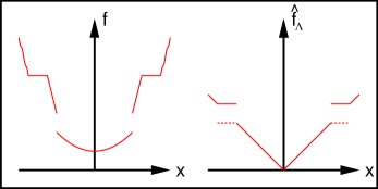
Figure 1: Left: objective function $f:\mathbb{R}\to\mathbb{R}$ with plateau and jump. Right: corresponding spatial suboptimality $\widehat{f}_{\Lambda}^{<}$ (dotted) and $\widehat{f}_{\Lambda}^{\leq}$ (solid).

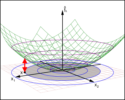
Figure 2: All relevant properties of the sphere function $f:\mathbb{R}^{2}\to\mathbb{R}$ for rank-based optimization are specified by its circular level sets, illustrated in blue on the domain (ground plane). The spatial sub-optimality of the point $x$ is the Lebesgue measure of the gray area, which coincides with the function value $\widehat{f}_{\Lambda}(x)$ indicated by the bold red vertical arrow. In this example it holds $\widehat{f}_{\Lambda}(x)=\pi\cdot\|x\|^{2}$, irrespective of the rank-preserving (and hence level-set preserving) transformation applied to $f$.

The definition is illustrated with two examples in figures 1 and 2. In the following, $m\in X$ will denote the elite (or parent) point, and $m^{(t)}$ is the elite point in iteration $t\in\mathbb{N}$ of an iterative algorithm, i.e., an evolutionary algorithm with $(1+\lambda)$ selection. For two very different reasons, namely 1) to avoid divergence of the algorithm in the case of unbounded search spaces, and 2) for simplicity of the technical arguments in the proofs, we restrict ourselves to the case that the sub-level set $S_{f}^{\leq}\big{(}m^{(0)}\big{)}$ of the initial iterate $m^{(0)}$ is bounded and has finite spatial sub-optimality. For most reasonable reference measures, boundedness implies finite spatial sub-optimality. For $X=\mathbb{R}^{d}$ equipped with the Lebesgue measure this is equivalent to the topological closure $\overline{S_{f}^{\leq}\big{(}m^{(0)}\big{)}}$ being compact. The assumptions immediately imply that $S_{f}^{<}(y)$ and $S_{f}^{\leq}(y)$ are bounded for all $y\leq f\big{(}m^{(0)}\big{)}$, and that restricted to $S_{f}^{\leq}(m^{(0)})$ the functions $\widehat{f}_{\Lambda}^{<}$ and $\widehat{f}_{\Lambda}^{\leq}$ take values in the bounded range $\big{[}0,\widehat{f}_{\Lambda}\big{(}m^{(0)}\big{)}\big{]}$. Since an elitist algorithm never accepts points outside $S_{f}^{\leq}(m^{(0)})$, we will from here on ignore the issue of infinite $\widehat{f}_{\Lambda}$-values.

In the continuous case, a plateau is a level set of positive Lebesgue measure. When defining a local optimum as the best point within an open neighborhood, then an interior point of a plateau is a local optimum, which may not always be intended. Anyway, when analyzing the (1+1)-ES we will not handle plateaus and instead assume that level sets of $f$ are zero sets. This also implies that $\widehat{f}_{\Lambda}^{\leq}$ and $\widehat{f}_{\Lambda}^{<}$ agree.

• Let $f:X\to\mathbb{R}$ be measurable. If $\widehat{f}_{\Lambda}^{\leq}(x)$ is finite for all $x\in X$ then it holds $\widehat{f}_{\Lambda}^{\leq}\widehat{\sim}f\widehat{\sim}\widehat{f}_{\Lambda}^{<}$.

The proof is found in the appendix. We use $\widehat{f}_{\Lambda}^{\leq}$ and $\widehat{f}_{\Lambda}^{<}$ (or simply $\widehat{f}_{\Lambda}$ if possible) as a canonical representative of its equivalence class (if the function values are finite, but see the discussion above). These functions have the property

$$\widehat{f}_{\Lambda}^{\leq}(x)=\Lambda\big{(}S_{\widehat{f}_{\Lambda}^{\leq}}(x)\big{)}\qquad\widehat{f}_{\Lambda}^{<}(x)=\Lambda\big{(}S_{\widehat{f}_{\Lambda}^{<}}(x)\big{)}$$

i.e., $\widehat{f}_{\Lambda}$ encodes the Lebesgue measure of its own sub-level sets. We will measure optimization progress in terms of $\widehat{f}_{\Lambda}$-values. Decreasing the spatial suboptimality $\widehat{f}_{\Lambda}$ by $\delta>0$ amounts to reducing the volume of better points by $\delta$.

Due to the rank-based nature of the algorithms under study we cannot expect to fulfill a sufficient decrease condition based on $f$-values. This is because a functional gain $\Delta:=f(x)-f(x^{\prime})>0$ achieved by moving from $x$ to $x^{\prime}$ can be reduced to an arbitrarily small or large gain $\varphi(f(x))-\varphi(f(x^{\prime}))$, where $\varphi$ is strictly monotonically increasing, and the class of transformations does not allow to bound the difference uniformly, neither additively nor multiplicatively. Instead, the following theorem establishes a progress or decrease guarantee measured in terms of the spatial suboptimality function $\widehat{f}_{\Lambda}$. It gets around the problem of inconclusive values in objective space (which, in case of single-objective optimization, is just the real line) by considering a quantity in search space, namely the reference measure of the sub-level set.

The algorithm is randomized, hence the decrease follows a distribution. The following definition captures properties of this distribution.

• Let $P$ denote a probability distribution on $X$ with a bounded density with respect to $\Lambda$ and let $f:X\to\mathbb{R}$ be a measurable objective function. The quantity

  $$u:=\sup\left\{\left.\frac{P(A)}{\Lambda(A)}\,\right|\,A\subset X\text{ measurable with }\Lambda(A)>0\right\}$$

  is an upper bound on the density. Consider a sample $x\sim P$. Define the functions

  $$r^{<}:\mathbb{R}\to[0,1],\qquad z\mapsto\Pr\big{(}f(x)<z\big{)}=P\left(S_{f}^{<}(z)\right)$$

  $$r^{\leq}:\mathbb{R}\to[0,1],\qquad z\mapsto\Pr\big{(}f(x)\leq z\big{)}=P\left(S_{f}^{\leq}(z)\right)$$

  of probabilities of strict and weak improvements. Furthermore, we define $s:[0,1]\to\mathbb{R}$ as a measurable inverse function fulfilling $r^{<}\big{(}s(q)\big{)}\leq q\leq r^{\leq}\big{(}s(q)\big{)}$ for all $q\in[0,1]$. We collect the discontinuities of $r^{<}$ and $r^{\leq}$ in the set $Z:=\big{\{}z\in\mathbb{R}\,\big{|}\,r^{<}(z)<r^{\leq}(z)\big{\}}$ and define the sum

  $$\zeta:=\sum_{z\in Z}\Big{(}r^{\leq}(z)-r^{<}(z)\Big{)}^{2}$$

  of squared improvement jumps.

Note that $u$, $r^{<}$, $r^{\leq}$, $s$, $Z$, and $\zeta$ implicitly depend on $\Lambda$, $P$, and $f$. This is not indicated explicitly in order to avoid excessive clutter in the notation.

If the function $f$ is continuous with continuous domain $X$ and without plateaus, then $r^{<}$ and $r^{\leq}$ coincide, we have $\zeta=0$, and $s$ maps each probability $q\in[0,1]$ to the corresponding unique quantile of the distribution of $f(x)$ under $P$. However, if there exists a plateau within the support of $P$ (a level set of positive $P$-measure, i.e., if $X$ is discrete), then $\zeta$ is positive and on $Z$ the function $s$ takes values anywhere between the lower quantile $P(f(x)<z)$ and the upper quantile $P(f(x)\leq z)$. The exact value does not matter, since the only use of $s$-values is as arguments to one of the $r$-functions. Indeed, $r^{<}(s(q))$ and $r^{\leq}(s(q))$ “round” the probability $q$ down or up, respectively, to the closest value that is attainable as the probability of sampling a sub-level set. The freedom in the choice of $s$ can also be understood in the context of figure 1: if the point $z$ in the definitions of $r^{<}$ and $r^{\leq}$ is located on the plateau, then $s(q)$ can be the anywhere between the probability mass of the sub-level set excluding and including the plateau.

With these definitions in place, the following theorem controls the expected value as well as the quantiles of the decrease distribution.

• Let $P$ denote a probability distribution on $X$ with a bounded density with respect to $\Lambda$ and let $f:X\to\mathbb{R}$ be a measurable objective function. We use the notation of the above definition. Fix a reference point $m\in X$ and let $p:=r^{<}\big{(}f(m)\big{)}$ denote the probability of strict improvement of a sample $x\sim P$ over $m$. Then for each $q\in[0,p]$, the $q$-quantile of the $\widehat{f}_{\Lambda}^{<}$-decrease is bounded from below by $\frac{p-r^{<}\big{(}s(q)\big{)}}{u}$ and the $q$-quantile of the $\widehat{f}_{\Lambda}^{\leq}$-decrease is bounded by $\frac{p-r^{\leq}\big{(}s(q)\big{)}}{u}+\Lambda\big{(}L_{f}(m)\big{)}$, i.e.,

  $$\Pr\left(\widehat{f}_{\Lambda}^{<}(m)-\widehat{f}_{\Lambda}^{<}(x)\geq\frac{p-r^{<}\big{(}s(q)\big{)}}{u}\right)\geq q,$$

  $$\Pr\left(\widehat{f}_{\Lambda}^{\leq}(m)-\widehat{f}_{\Lambda}^{\leq}(x)\geq\frac{p-r^{\leq}\big{(}s(q)\big{)}}{u}+\Lambda\big{(}L_{f}(m)\big{)}\right)\geq q.$$

  The expected $\widehat{f}_{\Lambda}^{<}$-decrease is bounded from below by

  $$\mathbb{E}\Big{[}\max\big{\{}0,\widehat{f}_{\Lambda}^{<}(m)-\widehat{f}_{\Lambda}^{<}(x)\big{\}}\Big{]}\geq\frac{p^{2}+\zeta}{2u},$$

  and the expected $\widehat{f}_{\Lambda}^{\leq}$-decrease is bounded from below by

  $$\mathbb{E}\Big{[}\max\big{\{}0,\widehat{f}_{\Lambda}^{\leq}(m)-\widehat{f}_{\Lambda}^{\leq}(x)\big{\}}\Big{]}\geq\frac{p^{2}+\zeta}{2u}+\Lambda\big{(}L_{f}(m)\big{)}.$$

• We start with the first two claims, which provide lower bounds on the $q$-quantiles of probabilities of improvement by some margin $\delta\geq 0$. The argument here is elementary: an $\widehat{f}_{\Lambda}$-improvement of $\delta$ from $m$ to $x$ means that the $\widehat{f}_{\Lambda}$-sub-level set of $x$ is smaller than that of $m$ by $\Lambda$-mass $\delta$ (due to the offspring $x$ improving upon its parent $m$). This corresponds to a difference in $P$-mass of the same $\widehat{f}_{\Lambda}$-sub-level sets of at most $u\cdot\delta$, which will correspond to $q$ in the following. Note that the probabilities ($\Pr(\dots)$-notation) correspond to the same distribution $P$ from which $x$ is sampled, and that $\widehat{f}_{\Lambda}$-values and $s$-values directly correspond to $\Lambda$-mass. The situation is illustrated in figure 3.

  To make the above argument precise we fix $q$ and define the $f$-level

  $$y_{q}:=\inf\Bigg{(}\Big{\{}y\in\mathbb{R}\,\Big{|}\,P(S_{f}^{\leq}(y))\geq q\Big{\}}\Bigg{)}.$$

  For $q=0$ the first two statements are trivial. For $q>0$ the infimum is attained and it thus holds $P\big{(}S_{f}^{\leq}(y_{q})\big{)}\geq q$. We define three disjoint sets: $A:=S_{f}^{<}(y_{q})$, $B:=L_{f}(y_{q})$, and $C:=S_{f}^{<}(m)\setminus S_{f}^{\leq}(y_{q})$. The nested sub-level sets $S_{f}^{<}(y_{q})=A$, $S_{f}^{\leq}(y_{q})=A\cup B$, and $S_{f}^{<}(m)=A\cup B\cup C$ are unions of these sets. By the definitions of $p$ and $q$ the probability of the set $C$ is upper bounded by $P(C)=P(S_{f}^{<}(m))-P(S_{f}^{\leq}(y_{q}))\leq p-q$, and the probability of $A\cup B$ is lower bounded by $P(A\cup B)\geq q$.

  We will show that the event of interest for the first claim, namely $\widehat{f}_{\Lambda}^{<}(m)-\widehat{f}_{\Lambda}^{<}(x)\geq\frac{p-r^{<}(s(q))}{u}$, implies $x\in S_{f}^{\leq}(y_{q})=A\cup B$. To this end we define the $\widehat{f}_{\Lambda}^{<}$-level $z_{q}^{<}:=\widehat{f}_{\Lambda}^{<}(m)-\frac{p-r^{<}(s(q))}{u}$ and the set $\Delta_{q}^{<}:=S_{\widehat{f}_{\Lambda}^{<}}^{<}(m)\setminus S_{\widehat{f}_{\Lambda}^{<}}^{\leq}(z_{q}^{<})$. We have

  $$\Lambda(\Delta_{q}^{<}) =\underbrace{\Lambda\left(S_{\widehat{f}_{\Lambda}^{<}}^{<}(m)\right)}_{=\widehat{f}_{\Lambda}^{<}(m)}-\underbrace{\Lambda\left(S_{\widehat{f}_{\Lambda}^{<}}^{\leq}(z_{q}^{<})\right)}_{\geq\widehat{f}_{\Lambda}^{<}(m)-\frac{p-r^{<}(s(q))}{u}}\leq\frac{p-r^{<}(s(q))}{u},$$

  and hence $P(\Delta_{q}^{<})\leq p-r^{<}(s(q))$ by the definition of $u$. Together with Lemma 2 this implies $\Delta_{q}^{<}\subset B\cup C$, and hence $A\subset S_{\widehat{f}_{\Lambda}^{<}}^{\leq}(z_{q}^{<})$. However, due to the definition of $S^{\leq}$ (in contrast to $S^{<}$), the sub-level set $A$ being a subset of $S_{\widehat{f}_{\Lambda}^{<}}^{\leq}(z_{q}^{<})$ implies that also the level set $B$ is contained in $S_{\widehat{f}_{\Lambda}^{<}}^{\leq}(z_{q}^{<})$. This shows the first claim.

  For the second claim we define the $\widehat{f}_{\Lambda}^{\leq}$-level $z_{q}^{\leq}:=\widehat{f}_{\Lambda}^{\leq}(m)-\frac{p-r^{\leq}(s(q))}{u}-\Lambda\big{(}L_{f}(m)\big{)}$ and the set $\Delta_{q}^{\leq}:=S_{\widehat{f}_{\Lambda}^{\leq}}^{<}(m)\setminus S_{\widehat{f}_{\Lambda}^{\leq}}^{\leq}(z_{q})$, and we note that it holds $\widehat{f}_{\Lambda}^{\leq}(m)-\Lambda\big{(}L_{f}(m)\big{)}=\widehat{f}_{\Lambda}^{<}(m)$. Then, with an analogous argument as above we obtain $P(\Delta_{q}^{<})\leq p-r^{\leq}(s(q))$. In this case we immediately arrive at $\Delta_{q}^{\leq}\subset C$ and hence at $A\cup B\subset S_{\widehat{f}_{\Lambda}^{\leq}}^{\leq}(z_{q}^{\leq})$, which shows the second claim.

  

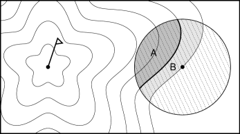
  Figure 3: Illustration of the quantile decrease, here in the continuous case. The optimum is marked with a flag. In this example, the level lines of the objective function $f$ are star-shaped. The circle with the dashed shading on the right indicates the sampling distribution, which has ball-shaped support in this case. The probability of the area $A\cup B$ is the value $p=P(A\cup B)$, and $q=P(A)$ is the probability of the event of interest, corresponding to a significant improvement. The area $\Lambda(B)$ is a lower bound on the improvement in terms of $\widehat{f}_{\Lambda}$. It is lower bounded by $\frac{P(B)}{u}=\frac{p-q}{u}$. The (bold) level line separating $A$ and $B$ belongs to $A$, and not to $B$. Therefore, if this set has positive measure, then we can only guarantee $q\leq P(A)$ (in contrast to equality), and the lower bound becomes $\frac{p-r^{<}(s(q))}{u}\leq\Lambda(B)$.

Let $Q$ denote the quantile function (the generalized inverse of the cdf) of the $\widehat{f}_{\Lambda}^{<}$-improvement $\max\big{\{}0,\widehat{f}_{\Lambda}^{<}(m)-\widehat{f}_{\Lambda}^{<}(x)\big{\}}$. Then the expectation is lower bounded by

$$\mathbb{E}\Big{[}\max\big{\{}0,\widehat{f}_{\Lambda}^{<}(m)-\widehat{f}_{\Lambda}^{<}(x)\big{\}}\Big{]}= \int_{0}^{1}Q(q)\,dq$$

$$\geq \int_{0}^{p}\frac{p-r^{<}\big{(}s(q)\big{)}}{u}\,dq$$

$$= \int_{0}^{p}\frac{p-q}{u}\,dq+\int_{0}^{p}\frac{q-r^{<}\big{(}s(q)\big{)}}{u}\,dq$$

$$= \int_{0}^{p}\frac{p-q}{u}\,dq+\sum_{z\in Z}\int_{r^{<}(z)}^{r^{\leq}(z)}\frac{q-r^{<}(z)}{u}\,dq$$

$$= \frac{p^{2}}{2u}+\sum_{z\in Z}\frac{\big{(}r^{\leq}(z)-r^{<}(z)\big{)}^{2}}{2u}$$

$$= \frac{p^{2}+\zeta}{2u}.$$

The proof of the expected $\widehat{f}_{\Lambda}^{\leq}$ improvement is analogous. The additional term $\Lambda\big{(}L_{f}(m)\big{)}$ again comes from $\widehat{f}_{\Lambda}^{\leq}(m)=\widehat{f}_{\Lambda}^{<}(m)+\Lambda\big{(}L_{f}(m)\big{)}$.       

In a $(1+\lambda)$ evolutionary algorithm, the reference point $m$ is usually the current best iterate (parent), and the distribution $P$ is the search distribution, from which the offspring are sampled. Our main application is the (1+1)-ES, where $x$ corresponds to the offspring point sampled from a Gaussian centered on $m$.

Due to the term $\Lambda\big{(}L_{f}(m)\big{)}$ in the decrease of $\widehat{f}_{\Lambda}^{\leq}$, the theorem covers the fitness-level method (Droste et al., , 2002; Wegener, , 2003). However, in particular for search distributions spreading their probability mass over many level sets, the theorem is considerably stronger.

In the continuous case, in the absence of plateaus, the statement can be simplified considerably:

• Under the assumptions and with the notation of definition 2 and theorem 2 we assume in addition that all level sets of $f$ have measure zero. Then for each $q\in[0,p]$, the $q$-quantile of the $\widehat{f}_{\Lambda}$-decrease is bounded from below by

  $$\Pr\left(\widehat{f}_{\Lambda}(m)-\widehat{f}_{\Lambda}(x)\geq\frac{p-q}{u}\right)\geq q,$$

  and the expected $\widehat{f}_{\Lambda}$-decrease is bounded from below by

  $$\mathbb{E}\Big{[}\max\big{\{}0,\widehat{f}_{\Lambda}(m)-\widehat{f}_{\Lambda}(x)\big{\}}\Big{]}\geq\frac{p^{2}}{2u}.$$

The following corollary is a broken down version for Gaussian search distributions $\mathcal{N}(m,C)$ with mean $m$ and covariance matrix $C$, which has the density

$$\varphi(x)=\frac{1}{(2\pi)^{d/2}\sqrt{\det(C)}}\exp\left(-\frac{1}{2}(x-m)^{T}C^{-1}(x-m)\right).$$

• Consider the search space $\mathbb{R}^{d}$ and the Lebesgue measure $\Lambda$. Let $f:\mathbb{R}^{d}\to\mathbb{R}$ denote a measurable objective function with level sets of measure zero. Consider a normally distributed sample $x\sim\mathcal{N}(m,C)$. Under the assumptions and with the notation of definition 2 and theorem 2, for each $q\in[0,p]$, the $q$-quantile of the $\widehat{f}_{\Lambda}$-decrease is bounded from below by

  $$\Pr\Big{(}\widehat{f}_{\Lambda}(m)-\widehat{f}_{\Lambda}(x)\geq(2\pi)^{d/2}\cdot\sqrt{\det(C)}\cdot(p-q)\Big{)}\geq q,$$

  and the expected $\widehat{f}_{\Lambda}$-decrease is bounded from below by

  $$\mathbb{E}\Big{[}\max\big{\{}0,\widehat{f}_{\Lambda}(m)-\widehat{f}_{\Lambda}(x)\big{\}}\Big{]}\geq(2\pi)^{d/2}\cdot\sqrt{\det(C)}\cdot\frac{p^{2}}{2}.$$

An isotropic distribution with component-wise standard deviation (step size) $\sigma>0$ has covariance matrix $C=\sigma^{2}I$, where $I\in\mathbb{R}^{d\times d}$ is the identity matrix; hence we have $\sqrt{\det(C)}=\sigma^{d}$. In the context of continuous search spaces, Jägersküpper, (2003) refers to $\widehat{f}_{\Lambda}$-progress as “spatial gain”. He analyzes in detail the gain distribution of an isotropic search distribution on the sphere model. This result is much less general than the previous corollary, since we can deal with arbitrary objective functions, which are characterized (locally) only by a single number, the success probability. For the special case of a Gaussian mutation and the sphere function, Jägersküpper’s computation of the spatial gain is more exact, since it is tightly tailored to the geometry of the case, in contrast to being based on a general bound. We lose only a multiplicative factor of the gain, which does not impact our analysis significantly. However, it should be noted that in the problem analyzed by Jägersküpper, the factor grows with the problem dimension $d$. The spatial gain is closely connected to the notion of a progress rate (Rechenberg, , 1973), in particular if the gain is lower bounded by a fixed fraction of the suboptimality. For a fixed objective function like the sphere model $f(x)=\|x\|^{2}$ it is easy to relate functional suboptimality $f(x)-f^{*}$ to spatial suboptimality $\widehat{f}_{\Lambda}(x)$.

The above statements apply immediately to evolutionary algorithms with (1+1) selection. Generalizing them to the best out of $\lambda$ samples is rather straightforward (based on well-known statements on the distribution of the minimum of $\lambda$ i.i.d. samples), resulting in bounds for the one-step behavior of elitist algorithms with $(1+\lambda)$ selection. This is not done here because we are not primarily interested in the scaling with $\lambda$, which is usually non-essential for the question whether or not a $(1+\lambda)$ algorithm converges to a (local) optimum.

3 Success-bases Step Size Control in the (1+1)-ES

In this section we discuss properties of the (1+1)-ES algorithm and provide an analysis of its success-based step size adaptation rule that will allow us to derive global convergence theorems. To this end we introduce a non-standard regularity property.

From here on, we consider the search space $\mathbb{R}^{d}$, equipped with the standard Borel $\sigma$-algebra, and $\Lambda$ denotes the Lebesgue measure. Of course, all results from the previous section apply, with $X=\mathbb{R}^{d}$.

In each iteration $t\in\mathbb{N}$, the state of the (1+1)-ES is given by $(m^{(t)},\sigma^{(t)})\in\mathbb{R}^{d}\times\mathbb{R}^{+}$. It samples one candidate offspring from the isotropic normal distribution $x^{(t)}\sim\mathcal{N}(m^{(t)},\big{(}\sigma^{(t)})^{2}I\big{)}$. The parent is replaced by successful offspring, meaning that the offspring must perform at least as good as the parent.

The goal of success-based step size adaptation is to maintain a stable distribution of the success rate, for example concentrated around $1/5$. This can be achieved with a number of different mechanisms. Here we consider the maybe simplest such mechanism, namely immediate adaptation based on “success” or “failure” of each sample. Pseudocode for the full algorithm is provided in Algorithm 1.

The constants $c_{-}<0$ and $c_{+}>0$ in Algorithm 1 control the change of $\log(\sigma)$ in case of failure and success, respectively. They are parameters of the method. For $c_{+}+4\cdot c_{-}=0$ we obtain an implementation of Rechenberg’s classic $1/5$-rule (Rechenberg, , 1973). We call $\tau=\frac{c_{-}}{c_{-}-c_{+}}$ the target success probability of the algorithm, which is always assumed to be strictly less than $1/2$. This is equivalent to $c_{+}>-c_{-}$. A reasonable parameter setting is $c_{-},c_{+}\in\Omega\left(\frac{1}{d}\right)$.

Two properties of the algorithm are central for our analysis: it is rank-based and it performs elitist selection, ensuring that the best-so-far solution is never lost and the sequence $f(m^{(t)})$ is monotonically decreasing.

Since step-size control depends crucially on the concept of a fixed rate of successful offspring, we define the success probability of the algorithm, which is the probability of a sampled point outperforming the parent in the search distribution center.

• For a measurable function $f:\mathbb{R}^{d}\to\mathbb{R}$, we define the success probability functions

  $$p_{f}^{<}:\mathbb{R}^{d}\times\mathbb{R}^{+}\to[0,1],\quad(m,\sigma)\mapsto \Pr\Big{(}f(x)<f(m)\,\Big{|}\,x\in\mathcal{N}(m,\sigma^{2}I)\Big{)}$$

  $$= \int_{S_{f}^{<}(m)}\frac{1}{(2\pi)^{d/2}\sigma^{d}}\cdot\exp\left(-\frac{\|x-m\|^{2}}{2\sigma^{2}}\right)\,dx,$$

  $$p_{f}^{\leq}:\mathbb{R}^{d}\times\mathbb{R}^{+}\to[0,1],\quad(m,\sigma)\mapsto \Pr\Big{(}f(x)\leq f(m)\,\Big{|}\,x\in\mathcal{N}(m,\sigma^{2}I)\Big{)}$$

  $$= \int_{S_{f}^{\leq}(m)}\frac{1}{(2\pi)^{d/2}\sigma^{d}}\cdot\exp\left(-\frac{\|x-m\|^{2}}{2\sigma^{2}}\right)\,dx.$$

The function $p_{f}^{\leq}$ computes the probability of sampling a point at least as good as $m$, while $p_{f}^{<}$ computes the probability of sampling a strictly better point. If $p_{f}^{<}$ and $p_{f}^{\leq}$ coincide (i.e., if there are no plateaus), then we write $p_{f}$. A nice property of the success probability is that it does not drop too quickly when increasing the step size:

• For all $m\in\mathbb{R}^{d}$, $\sigma>0$ and $a\geq 1$ it holds

  $$p_{f}^{<}(m,a\cdot\sigma) \geq\frac{1}{a^{d}}\cdot p_{f}^{<}(m,\sigma),$$

  $$p_{f}^{\leq}(m,a\cdot\sigma) \geq\frac{1}{a^{d}}\cdot p_{f}^{\leq}(m,\sigma).$$

The proof is found in the appendix; this is the case for a number of technical lemmas in this section. The next step is to define a plausible range for the step size.

• For $p\in[0,1]$ and a measurable function $f:\mathbb{R}^{d}\to\mathbb{R}$, we define upper and lower bounds

  $$\xi_{p}^{f}(m):=\inf \Big{\{}\sigma\in\mathbb{R}^{+}\,\Big{|}\,p_{f}^{<}(m,\sigma)\leq p\Big{\}}$$

  $$\eta_{p}^{f}(m):=\sup \Big{\{}\sigma\in\mathbb{R}^{+}\,\Big{|}\,p_{f}^{\leq}(m,\sigma)\geq p\Big{\}}$$

  on the step size guaranteeing lower and upper bounds on the probability of improvement.

We think of $\xi_{p}^{f}(m)$ with $p>\tau$ as a “too small” step size at $m$. Similarly, for $p<\tau$, $\eta_{p}^{f}(m)$ is a “too large” step size at $m$. Assume that the two values of $p$ are chosen so that a sufficiently wide range of “well-adapted” step sizes exists in between the “too small” and “too large” ones. We aim to establish that if the step size is outside this range then step size adaptation will push it back into the range. The main complication is that the range for $\sigma$ depends on the point $m$.

The following lemma establishes a gap between lower and upper step size bound, i.e., a lower bound on the size of the step size range.

• For $0\leq p_{H}\leq p_{T}\leq 1$ it holds $\sqrt[d]{p_{H}}\cdot\xi_{p_{T}}^{f}(x)\leq\sqrt[d]{p_{T}}\cdot\eta_{p_{H}}^{f}(x)$ for all $x\in\mathbb{R}^{d}$.

The following definition is central. It captures the ability of the (1+1)-ES to recover from a state with a far too small step size. This property is needed to avoid premature convergence.

• For $p>0$, a function $f:\mathbb{R}^{d}\to\mathbb{R}$ is called $p$-improvable in $x\in\mathbb{R}^{d}$ if $\xi_{p}^{f}(x)$ is positive. The function is called $p$-improvable on $Y\subset\mathbb{R}^{d}$ if $\xi_{p}^{f}\big{|}_{Y}$ (the function $\xi_{p}^{f}$ restricted to $Y$) is lower bounded by a positive, lower semi-continuous function $\tilde{\xi}_{p}^{f}:Y\to(0,1]$. A point $x\in\mathbb{R}^{d}$ is called $p$-critical if it is not $p$-improvable for any $p>0$.

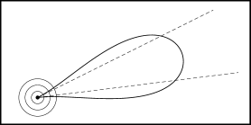
Figure 4: Illustration of a contour line with a kink opening up in an angle indicated by the dashed lines. The circles are iso-density lines on the isotropic Gaussian search distribution centered on the kink.

The property of $p$-improvability is a non-standard regularity condition. The concept applies to measurable functions, hence we do not need to restrict ourselves to smooth or continuous objectives. On the one hand side, the property excludes many measurable and even a few smooth functions. On the other hand, it is far less restrictive than continuity and smoothness, since it allows the objective function to jump and the level sets to have kinks. Intuitively, in the two-dimensional case illustrated in figure 4, if for each point the sub-level set opens up in an angle of more than $2\pi p$, then the function is $p$-improvable. This is the case for many discontinuous functions, however, not for all smooth ones. The degree three polynomial $f(x_{1},x_{2})=x_{1}^{3}+x_{2}^{2}$ can serve as a counter example, since the point $(0,0)$ is $p$-critical, with its level set forming a cuspidal cubic, see figure 6 in section 5.3. Local optima are always $p$-critical, but many critical points of smooth functions are not (see below). The above example demonstrates that some saddle points share this property, however, if $x$ is $p$-critical but not locally optimal then $p_{f}^{<}(x,\sigma)>0$ for all $\sigma>0$. This means that such a point can be improved with positive probability for each choice of the step size, but in the limit $\sigma\to 0$ the probability of improvement tends to zero.

We should stress the difference between point-wise $p$-improvability, which simply demands that $\xi_{p}^{f}$ is positive, and set-wise $p$-improvability, which in addition demands that $\xi_{p}^{f}$ is lower bounded by a lower semi-continuous positive function. The latter property ensures the existence of a positive lower bound for $\xi_{p}^{f}$ on a compact set. In this sense, set-wise $p$-improvability is uniform on compact sets. In sections 5.5 and 5.6 we will see examples where this makes a decisive difference.

Intuitively, the value of $p$ of a $p$-improvable function is critical: if it is below $\tau$ then the algorithm may be endangered to systematically decrease its step size while it should better do the contrary.

The next lemma establishes that smooth functions are $p$-improvable in all regular points, and also in most saddle points.

• Let $f:\mathbb{R}^{d}\to\mathbb{R}$ be continuously differentiable.

  1. For a regular point $x\in\mathbb{R}^{d}$, $f$ is $p$-improvable in $x$ for all $p<\frac{1}{2}$.

  2. Let $Y$ denote the set of all regular points of $f$, then $f$ is $p$-improvable on $Y$, for all $p<\frac{1}{2}$.

  3. Let $x\in\mathbb{R}^{d}$ denote a critical point of $f$, let $f$ be twice continuously differentiable in a neighborhood of $x$, and let $H=\nabla^{2}f(x)$ denote the Hessian matrix. If $H$ has at least one negative eigen value, then $x$ is not $p$-critical.

Similarly, we need to ensure that the step size does not diverge to $\infty$. This is easy, since the spatial suboptimality is finite:

• Consider the state $(m^{(t)},\sigma^{(t)})$ of the (1+1)-ES. For each $p\in(0,1)$, if

  $$\sigma^{(t)}\geq\sqrt[d]{\frac{\widehat{f}_{\Lambda}(m^{(t)})}{p\cdot(2\pi)^{d/2}}}$$

  then $p_{f}^{<}(m^{(t)},\sigma^{(t)})\leq p$.

In other words, a too large step size is very likely to produce unsuccessful offspring. The probability of success decays quickly with growing step size, since the step size bound grows slowly in the form $\Theta(p^{-1/d})$ as the success probability $p$ decays to zero. Applying the above inequality to $p<\tau$ implies that for large enough step size $\sigma^{(t)}$, the expected change $\mathbb{E}[\log(\sigma^{(t+1)})-\log(\sigma^{(t)})]$ in the (1+1)-ES (algorithm 1) is negative.

The following lemma is elementary. It is used multiple times in proofs, with the interpretation of the event “1” meaning that a statement holds true. It has a similar role as drift theorems in an analysis of the expected or high-probability behavior (Lehre and Witt, , 2013; Lengler and Steger, , 2016; Akimoto et al., , 2018), however, here we aim for almost sure results.

• Let $X^{(t)}\in\{0,1\}$ denote a sequence of independent binary random variables. If there exists a uniform lower bound $\Pr(X^{(t)}=1)\geq p>0$, then almost surely there exists an infinite sub-sequence $(t_{k})_{k\in\mathbb{N}}$ so that $X^{(t_{k})}=1$ for all $k\in\mathbb{N}$.

In applications of the lemma, the events of interest are not necessarily independent, however, they can be “made independent” by considering a sequence of independent events that imply the events of interest. In our applications this is the case if the events of actual interest hold with probability of at least $p$; then an i.i.d. sequence of Bernoulli events implying corresponding sub-events with probability of exactly $p$ does the job. In other words, we will have a sequence $\tilde{X}^{(t)}$ of independent events, where $\tilde{X}^{(t)}=1$ implies $X^{(t)}=1$. The above lemma is then applied to $\tilde{X}^{(t)}$, which trivially yields the same statement for $X^{(t)}$. We imply this construction in all applications of the lemma.

The following lemma establishes, under a number of technical conditions, that the step size control rule succeeds in keeping the step size stable. If the prerequisites are fulfilled then the result yields an impossible fact, namely that the overall reduction of the spatial suboptimality is unbounded. So the lemma is designed with proofs by contradiction in mind.

• Let $\big{(}m^{(t)},\sigma^{(t)}\big{)}$ denote the sequence of states of the (1+1)-ES on a measurable objective function $f:\mathbb{R}^{d}\to\mathbb{R}$. Let $p_{T},p_{H}\in(0,1)$ denote probabilities fulfilling $p_{H}<\tau<p_{T}$ and $\frac{p_{H}}{p_{T}}\leq e^{d\cdot c_{-}}$, and assume the existence of constants $0<b_{T}<b_{H}$ such that

  $$b_{T}\leq\xi_{p_{T}}^{f}(m^{(t)})\quad\text{and}\quad e^{c_{+}}\cdot\eta_{p_{H}}^{f}(m^{(t)})\leq b_{H}$$

  for all $t\in\mathbb{N}$. Then, with full probability, there exists an infinite sub-sequence $(t_{k})_{k\in\mathbb{N}}$ of iterations fulfilling

  $$\sigma^{(t_{k})}\in\Big{[}\xi_{p_{T}}^{f}\big{(}m^{(t_{k})}\big{)},\eta_{p_{H}}^{f}\big{(}m^{(t_{k})}\big{)}\Big{]}$$ (1)

  for all $k\in\mathbb{N}$.

Equation (1) is a rather weak condition demanding that step-size adaptation works as desired. However, the requirement of a uniform lower bound $b_{T}$ on the step size together with theorem 2 implies that the (1+1)-ES would make infinite $\widehat{f}_{\Lambda}$-progress in expectation. This is of course impossible if $\widehat{f}_{\Lambda}(m^{(0)})$ is finite, since $\widehat{f}_{\Lambda}$ is by definition non-negative. Therefore the lemma does not describe a typical situation observed when running the (1+1)-ES, but quite in contrast, an impossible situation that need to be excluded in the proof of the main result in the next section.

4 Global Convergence

In this section we establish our main result. The theorem ensures the existence of a limit point of the sequence $m^{(t)}$ in a subset of desirable locations. In many cases this amounts to convergence of the algorithm to a (local) optimum.

• Consider a measurable objective function $f:\mathbb{R}^{d}\to\mathbb{R}$ with level sets of measure zero. Assume that $K_{0}:=\overline{S_{f}^{\leq}\big{(}m^{(0)}\big{)}}$ is compact, and let $K_{1}\subset K_{0}$ denote a closed subset. If $f$ is $p$-improvable on $K_{0}\setminus K_{1}$ for some $p>\tau$, then the sequence $\big{(}m^{(t)}\big{)}_{t\in\mathbb{N}}$ has a limit point in $K_{1}$.

• Lemma 3 ensures the existence of $0<p_{H}<e^{-d\cdot c_{-}}\cdot\tau$ and

  $$b_{H}:=\sqrt[d]{\frac{\widehat{f}_{\Lambda}\big{(}m^{(0)}\big{)}}{p_{H}\cdot(2\pi)^{d/2}}}$$

  such that it holds $\eta_{p_{H}}^{f}(x)\leq b_{H}$ uniformly for all $x\in K_{0}$. In particular, $b_{H}$ is a uniform upper bound on $\eta_{p_{H}}^{f}$.

  Let $B(x,r)$ denote the open ball of radius $r>0$ around $x\in\mathbb{R}^{d}$ and define the compact set

  $$K(r):=K_{0}\mathbin{\Big{\backslash}}\bigcup_{x\in K_{1}}B(x,r).$$

  It holds $K(r)\subset K_{0}\setminus K_{1}$ and $\bigcup_{r>0}K(r)=K_{0}\setminus K_{1}$; hence $K(r)$ is a compact exhaustion of $K_{0}\setminus K_{1}$.

  Fix $r>0$, and assume for the sake of contradiction that all points $m^{(t)}$, $t>t_{0}$, are contained in $K(r)$. We set $p_{T}:=p$. Let $\tilde{\xi}_{p_{T}}^{f}$ denote the positive lower semi-continuous lower bound on $\xi_{p_{T}}^{f}$, which is guaranteed to exist due to the $p$-improvability of $f$. We define

  $$b_{T}:=\min\Big{\{}\tilde{\xi}_{p_{T}}^{f}(m)\,\Big{|}\,m\in K(r)\Big{\}}>0$$

  and apply lemma 3 to obtain an infinite sub-sequence of states with step size lower bounded by $\sigma^{(t)}\geq b_{T}>0$. According to lemma 3, the success probability is lower bounded by $p_{f}\big{(}m^{(t)},\sigma^{(t)}\big{)}\geq p_{I}:=(b_{T}/b_{H})^{d}\cdot p_{T}>0$ for all $m\in K(r)$ and $\sigma\in[b_{T},b_{H}]$.

  Corollary 2 ensures that in each such state the probability to decrease the $\widehat{f}_{\Lambda}$-value by at least $(2\pi)^{d/2}\cdot b_{T}^{d}\cdot p_{I}/2$ is lower bounded by $p_{I}/2>0$. We apply lemma 3 with the following construction. For each state $(m,\sigma)$ we pick a set $E(m,\sigma)\subset\mathbb{R}^{d}$ of probability mass $p_{I}/2$ improving on $\widehat{f}_{\Lambda}(m)$ by at least $(2\pi)^{d/2}\cdot b_{T}^{d}\cdot p_{I}/2$. Then we model the sampling procedure of the (1+1)-ES in iteration $t$ as a two-stage process: first we draw a binary variable $\tilde{X}^{(t)}\in\{0,1\}$ with $\Pr(\tilde{X}{(t)}=1)=p_{I}/2$, and then we draw $x^{(t)}$ from a Gaussian restricted to $E(m^{(t-1)},\sigma^{(t-1)})$ if $\tilde{X}{(t)}=1$, and restricted to the complement otherwise. The variables $\tilde{X}^{(t)}$ are independent, by construction.

  Then lemma 3 implies that the overall $\widehat{f}_{\Lambda}$-decrease is almost surely infinite, which contradicts the fact that $\widehat{f}_{\Lambda}(m^{(0)})$ is finite and $\widehat{f}_{\Lambda}$ is lower bounded by zero. Hence, the sequence $m^{(t)}$ leaves $K(r)$ after finitely many steps, almost surely. For $r=1/n$, let $t_{n}$ denote an iteration fulfilling $m^{(t_{n})}\not\in K(r)$. The sequence $\big{(}m^{(t_{n})}\big{)}_{n\in\mathbb{N}}$ does not have a limit point in $K_{0}\setminus K_{1}$ (since that point would be contained in $K(r)$ for some $r>0$), however, due to the Bolzano-Weierstraß theorem it has at least one limit point in $K_{0}$, which must therefore be located in $K_{1}$.       

The above theorem is of primary interest if $K_{1}$ is the set of (local) minima of $f$, or at least the set of critical or $p$-critical points. Due to the prerequisites of the theorem we always have

$$\overline{\Big{\{}x\in K_{0}\,\Big{|}\,x\text{ is $p$-critical}\Big{\}}}\subset K_{1},$$

i.e., $p$-critical points are candidate limit points.

In accordance with Akimoto et al., (2010), the following corollary establishes convergence to a critical point for continuously differentiable functions.

• Let $f:\mathbb{R}^{d}\to\mathbb{R}$ be a continuously differentiable function with level sets of measure zero. Assume that $K_{0}=\overline{S_{f}^{\leq}\big{(}m^{(0)}\big{)}}$ is compact. Then the sequence $\big{(}m^{(t)}\big{)}_{t\in\mathbb{N}}$ has a critical limit point.

• Define $K_{1}:=\{x\in K_{0}\,|\,\nabla f(x)=0\}$ as the set of critical points. This set is compact. Lemma 3 ensures that $f$ is $p$-improvable on $K_{0}\setminus K_{1}$ for all $p<1/2$. Then the claim follows immediately from theorem 4.       

Technically the above statements do not apply to problems with unbounded sub-level sets. However, due to the fast decay of the tails of Gaussian search distributions we can often approximate these problems by changing the function “very far away” from the initial search distribution, in order to make the sub-level sets bounded. We may then even apply the theorem with empty $K_{1}$, which implies that after a while the approximation becomes insufficient since the algorithm diverges. In this sense we can conclude divergence, e.g., on a linear function. We will use this argument several times in the next section, mainly to avoid unnecessary technical complications when defining saddle points and ridge functions.

We may ask whether $p$-improvability for $p>\tau$ is not only a sufficient but also a necessary condition for global convergence. This turns out to be wrong. The quadratic saddle point case discussed below in section 5.2 is a counter example, where the algorithm diverges reliably even if the success probability is far smaller than $\tau$. In contrast, the ridge of $p$-critical saddle points analyzed in section 5.3 results in premature convergence, despite the fact that the critical points form a zero set, and this can even happen for a ridge of $p$-improvable points with $p<\tau$, see section 5.4. Drift analysis is a promising tool for handling all of these cases. Here we provide a rather simple result, which still suffices for many interesting cases. A related analysis for a non-elitist ES was carried out by Beyer and Meyer-Nieberg, (2006).

• Consider a measurable objective function $f:\mathbb{R}^{d}\to\mathbb{R}$ with level sets of measure zero. Let $m\in\mathbb{R}^{d}$ be a $p$-critical point. If the success probability decays sufficiently quickly, i.e., if

  $$\sum_{k=0}^{\infty}p_{f}^{\leq}(m,e^{k\cdot c_{-}})<\infty$$

  then for each given $p<1$ there exists an initial condition such that the (1+1)-ES converges to $m$ with probability of at least $p$.

• Define the zero sequence $S_{K}:=\sum_{k=K}^{\infty}p_{f}^{\leq}(m,e^{k\cdot c_{-}})$. For given $p<1$, there exists a $K_{0}$ such that $S_{K_{0}}<1-p$. By definition, the probability of never sampling a successful offspring when starting the algorithm in the initial state $m^{(0)}=m$, $\sigma^{(0)}=e^{K_{0}\cdot c_{-}}$ is given by $S_{K_{0}}$; in this case we have $m^{(t)}=m$ for all $t\in\mathbb{N}$.       

The above theorem precludes global convergence to a (local) optimum with full probability in the presence of a suitable non-optimal $p$-critical point.

5 Case Studies

In this section we analyze various example problems with very different characteristics, by applying the above convergence analysis. We characterize the optimization behavior of the (1+1)-ES, giving either positive or negative results in terms of global convergence. We start with smooth functions and then turn to less regular cases of non-smooth and discontinuous functions. On the one hand side, we show that the theorem is applicable to interesting and non-trivial cases; on the other hand we explore its limits.

5.1 The 2-D Rosenbrock Function

The two-dimensional Rosenbrock function is given by

$$f(x_{1},x_{2}):=100(x_{1}^{2}-x_{2})^{2}+(x_{1}-1)^{2}.$$

This is a degree four polynomial. The function is unimodal (has a single local minimum), but not convex. Moreover, it does not have critical points other than the global optimum $x^{*}=(1,1)$. The function is illustrated in figure 5.

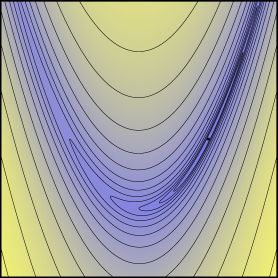
Figure 5: The 2-D Rosenbrock function in the range $[-2,2]\times[-1,3]$.

The Rosenbrock function is a popular test problem since it requires a diverse set of optimization behaviors: the algorithm must descend into a parabolic valley, follow the valley while adapting to its curved shape, and finally converge into the global optimum, which is a smooth optimum with non-trivial (but still moderate) conditioning.

Corollary 4 immediately implies convergence of the (1+1)-ES into the global optimum. It does not say anything about the speed of convergence, however, Jägersküpper, 2006a established linear convergence in the last phase with overwhelming probability (however, using a different step size adaptation rule).

Taken together, these results give a rather complete picture of the optimization process: irrespective of the initial state we know that the algorithm manages to locate the global optimum without getting stuck on the way. Once the objective function starts to look quadratic in good enough approximation, Jägersküpper’s result indicates that linear convergence can be expected. The same analysis applies to all twice continuously differentiable unimodal function without critical points other than the optimum.

5.2 Saddle Points—The $p$-improvable Case

We consider the quadratic objective function

$$f(x_{1},x_{2}):=a\cdot x_{1}^{2}-x_{2}^{2}$$

with parameter $a>0$. The origin is a saddle point. It is $p$-improvable for all $p<2\cot^{-1}(\sqrt{a})/\pi$ (see the appendix for details). For small enough $a$, the success probability is larger than $\tau$ and corollary 4 applies, while for large values of $a$ the success probability decays to zero and we lose all guarantees.

Simulations show that the ES overcomes the zero level set containing the saddle point without a problem, also for large values of $a$. It seems that $p$-improvable saddle points do not result in premature convergence of the algorithm, irrespective of the value of $p>0$. However, this statement is based on an empirical observation, not on a rigorous proof.

5.3 Saddle Points—The $p$-critical Case

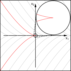
Figure 6: Level lines of the function $f(x_{1},x_{2})=x_{1}+|x_{2}|^{\frac{2}{3}}$ in the range $[-1,1]^{2}$. The inset shows a zoom of factor $10$.

The function

$$f(x_{1},x_{2})=x_{1}+|x_{2}|^{\frac{2}{3}}$$

models a ridge shaped after the zero set of the cubic polynomial $f(x_{1},x_{2}):=x_{1}^{3}+x_{2}^{2}$. It has $p$-critical saddle points on the line $\mathbb{R}\times\{0\}\subset\mathbb{R}^{2}$ forming a ridge, see figure 6. Without loss of generality we consider $m=0\in\mathbb{R}^{2}$ in the following. A successful offspring $x\in\mathbb{R}^{2}$ fulfills $x_{1}^{3}+x_{2}^{2}\leq 0$. For small enough $\sigma$ and hence for small enough $\|x\|\ll 1$, $\|x\|\in\Theta(\sigma)$, this implies $-x_{1}\gg|x_{2}|$ and hence $-x_{1}\in\Theta(\sigma)$ and $|x_{2}|\in o(\sigma)$. Plugging this into the above inequality we obtain $|x_{2}|\in\mathcal{O}(-x_{1}\cdot\sqrt{\sigma})$. Therefore, for small $\sigma$ we have $p_{f}^{\leq}(0,\sigma)\in\mathcal{O}(\sqrt{\sigma})$. This implies that the cumulative success probability

$$\sum_{t=0}^{\infty}p_{f}^{\leq}(0,e^{t\cdot c_{-}})=\mathcal{O}\left(\sum_{t=0}^{\infty}e^{t\cdot c_{-}/2}\right)=\mathcal{O}\left(\frac{1}{1-e^{c_{-}/2}}\right)=\mathcal{O}(1)$$

is finite, and theorem 4 yields (premature) convergence with arbitrarily high probability.

5.4 Linear Ridge

Consider the linear ridge objective

$$f(x_{1},x_{2}):=x_{1}+a\cdot|x_{2}|$$

with parameter $a>0$. The function is continuous, and its level sets contain a kink. Again, the line $\mathbb{R}\times\{0\}$ is critical; this is where the function is non-differentiable. The function is $p$-improvable for $p<\cot^{-1}(a)/\pi<1/2$ (see the appendix). For $a\to\infty$ the success probability decays to zero.

As long as $\cot^{-1}(a)/\pi>\tau$ we can conclude divergence of the algorithm (the intended behavior) from theorem 4. Otherwise we lose this property, and it is well known and easy to check with simulations that for large enough $a$ the algorithm indeed converges prematurely.

5.5 Sphere with Jump

Our next example is an “essentially discontinuous” problem in the sense that in general no function in the equivalence class $[f]$ is continuous. We consider objective functions of the form

$$f(x):=\|x\|^{2}+\mathds{1}_{S}(x),$$

where $\mathds{1}_{S}$ denotes the indicator function of a measurable set $S\subset\mathbb{R}^{d}$. If $S$ has a sufficiently simple shape then this problem is similar to a constrained problem where $S$ is the infeasible region (Arnold and Brauer, , 2008), at least for small enough $\sigma$. As long as $m^{(t)}\in S$ the (1+1)-ES essentially optimizes the sphere function, and as soon as $m^{(t)}\not\in S$ the (soft) constraint comes into play.

If $S$ is the complement of a star-shaped open neighborhood of the origin then it is easy to see that the function is unimodal and $p$-improvable for all $p<1/2$. Theorem 4 applied with $K_{1}:=\{0\}$ yields the existence of a sub-sequence converging to the origin, which implies convergence of the whole sequence due to monotonicity of $f\big{(}m^{(t)}\big{)}$. The results of Jägersküpper, (2005) and Akimoto et al., (2018) imply linear convergence.

Other shapes of $S$ give different results. For example, for $d\geq 2$, if $S$ is a ball not containing the origin then the function is still unimodal. For example, define $S$ as the open ball of radius $1/2$ around the first unit vector $e_{1}=(1,0,\dots,0)\in\mathbb{R}^{d}$. Then at $m:=3/2\cdot e_{1}$ we have $\xi_{p}^{f}(m)=0$ for all $p>0$, and according to theorem 4 the algorithm can converge prematurely if the step size is small. Alternatively, if $S$ is the closed ball, then all points except the origin are $p$-improvable for all $p<1/2$, however, there does not exist a positive lower semi-continuous lower bound on $\xi_{p}^{f}$ in any neighborhood of $m=3/2\cdot e_{1}$, and again the algorithm can converge to this point, irrespective of the target success probability $\tau$.

Now consider the strip $S:=(a,\infty)\times(0,1)\subset\mathbb{R}^{2}$ with parameter $a>0$. An elementary calculation of the success rate at $m:=(a+\varepsilon,1)$ for $\sigma\to 0$ shows that the (1+1)-ES is guaranteed to converge to the optimum irrespective of the initial conditions if $\tan^{-1}(a)/(2\pi)<\tau$ (details are found in the appendix), i.e., if $a$ is large enough; otherwise the algorithm can converge prematurely to a point on the edge $(a,\infty)\times\{1\}$ of $S$.

5.6 Extremely Rugged Barrier

Let us drive the above discontinuous problem to the extreme. Consider the one-dimensional problem

$$f(x):=x+\mathds{1}_{S}(x),$$

where $S\subset[-1,0]$ is a Smith-Volterra-Cantor set, also known as a fat Cantor set. $S$ is closed, has positive measure (usually chosen as $\Lambda(S)=1/2$), but is nowhere dense. Counter-intuitively, the function is unimodal in the sense that no point is optimal restricted to an open neighborhood (which is what commonly defines a local optimum). Still, intuitively, $S$ should act as a barrier blocking optimization progress with high probability.

The function is point-wise $p$-improvable everywhere. However, similar to the closed ball case in the previous section, there is no positive, lower semi-continuous lower bound on $\xi_{p}^{f}$. Therefore theorem 4 does not apply. Indeed, unsurprisingly, simulations show that the algorithm gets stuck with positive probability when initialized with $0<x^{(0)}\ll 1$ and $\sigma\ll 1$. When removing $0$ from $S$, then analogous to section 5.3 we obtain $p_{f}^{\leq}(m,\sigma)\in\mathcal{O}(\sqrt{\sigma})$ for $m=0$ and small $\sigma$, and hence theorem 4 applies.

In contrast, if $S$ is a Cantor set of measure zero then the algorithm diverges successfully, since it ignores zero sets with full probability.

6 Conclusions and Future Work

We have established global convergence of the (1+1)-ES for an extremely wide range of problems. Importantly, with the exception of a few proof details, the analysis captures the actual dynamics of the algorithm and hence consolidates our understanding of its working principles.

Our analysis rests on two pillars. The first one is a progress guarantee for rank-based evolutionary algorithms with elitist selection. In its simplest form, it bounds the progress on problems without plateaus from below. It seems to be quite generally applicable, e.g., to runtime analysis and hence to the analysis of convergence speed.

The second ingredient is an analysis of success-based step size control. The current method barely suffices to show global convergence. It is not suitable for deducing stronger statements like linear convergence on scale invariant problems. Control of the step size on general problems therefore needs further work.

Many natural questions remain open, the most significant are listed in the following. These open points are left for future work.

• The approach does not directly yield results on the speed of convergence. However, the progress guarantee of theorem 2 is a powerful tool for such an analysis. It can provide us with drift conditions and hence yield bounds on the expected runtime and on the tails of the runtime distribution. But for that to be effective we need better tools for bounding the tails of the step size distribution. Here, again, drift is a promising tool.

• The current results are limited to step-size adaptive algorithms and do not include covariance matrix adaptation. One could hope to extend the proceeding to the (1+1)-CMA-ES algorithm (Igel et al., , 2007), or to (1+1)-xNES (Glasmachers et al., , 2010). Controlling the stability of the covariance matrix is expected to be challenging. It is not clear whether additional assumptions will be required. As an added benefit, it may be possible to relax the condition $p>\tau$ for $p$-improvability, by requiring it only after successful adaptation of the covariance matrix.

• Plateaus are currently not handled. Theorem 2 shows how they distort the distribution of the decrease. Worse, they affect step size adaptation, and they make it virtually impossible to obtain a lower bound on the one-step probability of a strict improvement. Therefore, proper handling of plateaus requires additional arguments.

• In the interest of generality, our convergence theorem only guarantees the existence of a limit point, not convergence of the sequence as a whole. We believe that convergence actually holds in most cases of interest (at least as long as there are no plateaus, see above). This is nearly trivial if the limit point is an isolated local optimum, however, it is unclear for a spatially extended optimum, e.g., a low-dimensional variety or a Cantor set.

• Our current result requires a saddle point to be $p$-improvable for some $p>\tau$, otherwise the theorem does not exclude convergence of the ES to the saddle point. We know from simulations that the (1+1)-ES overcomes $p$-improvable saddle points reliably, also for $p\ll\tau$. A proper analysis guaranteeing this behavior would allow to establish statements analogous to work on gradient-based algorithms that overcome saddle points quickly and reliably, see e.g. Dauphin et al., (2014). However, this is clearly beyond the scope of the present paper.

• We provide only a minimal negative result stating that the algorithm may indeed converge prematurely with positive probability if there exists a $p$-critical point for which the cumulative success probability does not sum to infinity. In section 5.5 it becomes apparent that this notion is rather weak, since the statement is not formally applicable to the case of a closed ball, which however differs from the open ball scenario only on a zero set. This makes clear that there is still a gap between positive results (global convergence) and negative results (premature convergence). Theorem 4 can for sure be strengthened, but the exact conditions remain to be explored. A single $p$-improvable point with $p<\tau$ is apparently insufficient. A $p$-critical point may be sufficient, but it is not necessary.

Acknowledgments

I would like to thank Anne Auger for helpful discussions, and I gratefully acknowledge support by Dagstuhl seminar 17191 “Theory of Randomized Search Heuristics”.

Appendix

Here we provide the proofs of technical lemmas that were omitted from the main text in the interest of readability.

 

• We have to show that the level sets of all three functions agree outside a set of measure zero. It is immediately clear from definition 2 that the level sets of $f$ are a refinement of the level sets of $\widehat{f}_{\Lambda}^{\leq}$ and $\widehat{f}_{\Lambda}^{<}$, i.e., $f(x)=f(x^{\prime})$ implies $\widehat{f}_{\Lambda}^{\leq}(x)=\widehat{f}_{\Lambda}^{\leq}(x^{\prime})$ and $\widehat{f}_{\Lambda}^{<}(x)=\widehat{f}_{\Lambda}^{<}(x^{\prime})$, and $\widehat{f}_{\Lambda}^{\leq}(x)<\widehat{f}_{\Lambda}^{\leq}(x^{\prime})$ and $\widehat{f}_{\Lambda}^{<}(x)<\widehat{f}_{\Lambda}^{<}(x^{\prime})$ both imply $f(x)<f(x^{\prime})$.

  It remains to be shown that $\widehat{f}_{\Lambda}^{\leq}$ and $\widehat{f}_{\Lambda}^{<}$ do not join $f$-level sets of positive measure. Let $y\in\mathbb{R}$ denote a level so that $Y=\big{(}\widehat{f}_{\Lambda}^{<}\big{)}^{-1}(y)$ has positive measure $\Lambda(Y)>0$. We have to show that this measure (not necessarily the whole set, only up to a zero set) is covered by a single $f$-level set. Assume the contrary, for the sake of contradiction. Then we find ourselves in one of the following situations:

  1. There exist $x,x^{\prime}\in Y$ fulfilling $a:=f(x)<f(x^{\prime})=:a^{\prime}$ and it holds $\Lambda\big{(}f^{-1}(a)\big{)}>0$ and $\Lambda\big{(}f^{-1}(a^{\prime})\big{)}>0$. So the mass of $Y$ is split into at least two chunks of positive measure. This implies $\widehat{f}_{\Lambda}^{<}(x^{\prime})-\widehat{f}_{\Lambda}^{<}(x)\geq\Lambda\big{(}f^{-1}(a)\big{)}>0$, which contradicts the assumption that $x$ and $x^{\prime}$ belong to the same $\widehat{f}_{\Lambda}^{<}$-level.

  2. There exist $x,x^{\prime}\in Y$ fulfilling $a=f(x)<f(x^{\prime})=a^{\prime}$ and it holds $\Lambda\big{(}f^{-1}(I)\big{)}>0$ for the open interval $I=(a,a^{\prime})$. So $Y$ consists of a continuum of level sets of measure zero. Again, this implies $\widehat{f}_{\Lambda}^{<}(x^{\prime})-\widehat{f}_{\Lambda}^{<}(x)\geq\Lambda\big{(}f^{-1}(I)\big{)}>0$, leading to the same contradiction as in the first case.

  The argument for $\widehat{f}_{\Lambda}^{\leq}$ is exactly analogous.       

 

• It holds

  $$p_{f}^{<}(m,a\cdot\sigma) =\int_{S_{f}^{<}(m)}\frac{1}{(2\pi)^{d/2}a^{d}\sigma^{d}}\cdot\exp\left(-\frac{\|x-m\|^{2}}{2a^{2}\sigma^{2}}\right)\,dx$$

  $$\geq\frac{1}{a^{d}}\cdot\int_{S_{f}^{<}(m)}\frac{1}{(2\pi)^{d/2}\sigma^{d}}\cdot\exp\left(-\frac{\|x-m\|^{2}}{2\sigma^{2}}\right)\,dx$$

  $$=\frac{1}{a^{d}}\cdot p_{f}^{<}(m,\sigma).$$

  The computation for $p_{f}^{\leq}$ is analogous.       

 

• Fix $x$ and define $\xi:=\xi_{p_{T}}^{f}(x)$. The cases $p_{H}=0$ and $\xi=0$ are trivial, so in the following we treat the case that both are positive. For $a\geq 1$ it holds

  $$p_{T} =\phantom{a^{d}\cdot}\int_{S_{f}^{<}(x)}\frac{1}{(2\pi)^{d/2}\xi^{d}}\exp\left(-\frac{\|x^{\prime}-x\|^{2}}{2\xi^{2}}\right)\,dx^{\prime}$$

  $$=a^{d}\cdot\int_{S_{f}^{<}(x)}\frac{1}{(2\pi)^{d/2}a^{d}\xi^{d}}\exp\left(-\frac{\|x^{\prime}-x\|^{2}}{2\xi^{2}}\right)\,dx^{\prime}$$

  $$\leq a^{d}\cdot\int_{S_{f}^{<}(x)}\frac{1}{(2\pi)^{d/2}a^{d}\xi^{d}}\exp\left(-\frac{\|x^{\prime}-x\|^{2}}{2a^{2}\xi^{2}}\right)\,dx^{\prime}.$$

  In other words, the success probability for step size $a\cdot\xi$ is at least $p_{T}/a^{d}$. Hence, in order to push the success probability below $p_{T}/a^{d}$, the step size must be at least $\xi\cdot a$, which therefore bounds $\eta_{p_{T}/a^{d}}^{f}(x)$ from below. Applying the above argument with $a=\sqrt[d]{p_{T}/p_{H}}$ completes the proof.       

 

• In a small enough neighborhood of a regular point $x$ the function $f$ can be approximated arbitrarily well by a linear function (its first order Taylor polynomial). In particular, the level set of $f$ is arbitrarily well approximated by a hyperplane, for which the probability of strict improvement is exactly $1/2$. Hence we have

  $$\lim_{\sigma\to 0}p_{f}^{<}(x,\sigma)=\frac{1}{2},$$

  which immediately implies the first statement.

  We have already seen that the second statement holds point-wise. It remains to be shown that $\xi_{p}^{f}|_{Y}$ is lower bounded by a positive, lower semi-continuous function. To this end we show that $\xi_{p}^{f}$ itself is lower-semi-continuous, and we note that $\xi_{p}^{f}|_{Y}$ takes positive values. Consider a convergent sequence $(a_{t})_{t\in\mathbb{N}}\to x\in\mathbb{R}^{d}$ and define $\xi_{a}:=\lim\inf_{t\to\infty}\xi_{p}^{f}(a_{t})$ and $\xi_{x}:=\xi_{p}^{f}(x)$. We have to show that it holds $\xi_{x}\leq\xi_{a}$ for all choices of $x$ and $(a_{t})_{t\in\mathbb{N}}$. We define

  $$S_{x}:=\, \Big{\{}\sigma\in\mathbb{R}^{+}\,\Big{|}\,p^{<}_{f}(x,\sigma)\leq p\Big{\}}$$

  $$\text{and}\qquad S_{a}:=\, \Big{\{}\sigma\in\mathbb{R}^{+}\,\Big{|}\,\exists(t_{k})_{k\in\mathbb{N}}:\,p^{<}_{f}(a_{t_{k}},\sigma)\leq p\,\forall k\in\mathbb{N}\Big{\}},$$

  which allows us to write $\xi_{a}=\inf(S_{a})$ and $\xi_{x}=\inf(S_{x})$. Fix $\sigma\in S_{a}$ and a corresponding sub-sequence $(t_{k})_{k\in\mathbb{N}}$ so that it holds $p^{<}_{f}(a_{t_{k}},\sigma)\leq p\,\forall k\in\mathbb{N}$. From the continuity of $f$ it follows that the success probability function $p_{f}^{<}$ is lower semi-continuous (and even continuous in its second argument, the step size). From $\lim_{k\to\infty}a_{t_{k}}=x$ and lower semi-continuity of $p^{<}_{f}$ it follows $\sigma\in S_{x}$. We conclude $S_{a}\subset S_{x}$ and therefore $\xi_{x}\leq\xi_{a}$.

To show the last statement we construct a cone of improving steps centered at $x$. This cone makes up a fixed fraction of each ball centered on $x$, which shows that $x$ is $p$-improvable, where $p$ is any number smaller than the volume of the intersection of ball and cone divided by the volume of the ball, which is well-defined and positive in the limit when the radius tends to zero. Let $v$ denote an eigen vector of $H$ fulfilling $v^{T}Hv<0$. For $\sigma\to 0$, the objective function is well approximated by the quadratic Taylor expansion

$$f(x^{\prime})\approx g(x^{\prime})=f(x)+(x-x^{\prime})^{T}H(x-x^{\prime}).$$

The sub-level set $S_{f}^{<}(x)$ is locally well approximated by $S_{g}^{<}(x)$, which is a cone centered on $x$. Whether a ray $x+\mathbb{R}\cdot z$ belongs to $S_{g}^{<}(x)$ or not depends on whether $z^{T}Hz<0$ or not. Now, the eigen vector $v$ has this property, and due to continuity of $g$, the same holds for an open neighborhood $N$ of $v$. The cone $x+\mathbb{R}\cdot N$ is contained in $S_{g}^{<}(x)$ and has the same positive probability $s_{g}^{<}(x,\sigma)=p>0$ under $\mathcal{N}(x,\sigma^{2}I)$ for all $\sigma>0$. We conclude

$$\lim_{\sigma\to 0}p_{f}^{<}(x,\sigma)\geq p>0,$$

which completes the proof.       

 

• We use the short notation $m:=m^{(t)}$ and $\sigma=\sigma^{(t)}$. Let $S=S_{f}^{<}(m)$ denote the region of improvement, with Lebesgue measure $\widehat{f}_{\Lambda}(m)$. The probability of sampling from this region is bounded by

  $$p_{f}^{<}(m) =\int_{S}\frac{1}{(2\pi)^{d/2}\sigma^{d}}\exp\left(-\frac{\|x-m\|^{2}}{2\sigma^{2}}\right)\,\text{d}x$$

  $$=\frac{1}{(2\pi)^{d/2}\sigma^{d}}\int_{S}\exp\left(-\frac{\|x-m\|^{2}}{2\sigma^{2}}\right)\,\text{d}x$$

  $$<\frac{1}{(2\pi)^{d/2}\sigma^{d}}\int_{S}\text{d}x$$

  $$=\frac{\widehat{f}_{\Lambda}(m)}{(2\pi)^{d/2}\sigma^{d}}$$

  $$\leq p,$$

  where the last inequality is equivalent to the assumption.       

 

• Assume the contrary, for the sake of contradiction. Then

  $$\sum_{t=1}^{\infty}X^{(t)}<\infty.$$

  Fix $N\in\mathbb{N}$. Hoeffding’s inequality applied with $\varepsilon=p/2$ and $n\geq\frac{2N}{p}$ yields

  $$\Pr\left(\sum_{t=1}^{n}X^{(t)}\leq N\right)\leq\exp\left(-n\cdot\frac{p^{2}}{2}\right)\underset{n\to\infty}{\longrightarrow}0.$$

  Hence, for $n\to\infty$, with full probability the infinite sum exceeds $N$. Since $N$ was arbitrary, we arrive at a contradiction.       

 

• In each iteration, the step size $\sigma$ is multiplied by either $e^{c_{-}}$ or $e^{c_{+}}$. According to Lemma 3, the condition $\frac{p_{H}}{p_{T}}\leq e^{d\cdot c_{-}}$ yields

  $$\frac{\eta_{p_{H}}^{f}\big{(}m^{(t_{k})}\big{)}}{\xi_{p_{T}}^{f}\big{(}m^{(t_{k})}\big{)}}\geq e^{-c_{-}}.$$

  An unsuccessful step of the (1+1)-ES in iteration $t$ results in a reduction of the step size by the factor $\frac{\sigma^{(t+1)}}{\sigma^{(t)}}=e^{c_{-}}<1$ and leaves $m^{(t+1)}=m^{(t)}$ unchanged. We conclude that in no such step can overjump the interval $\big{[}\xi_{p_{T}}^{f}\big{(}m^{(t)}\big{)},\eta_{p_{H}}^{f}\big{(}m^{(t)}\big{)}\big{]}$, in the sense of $\sigma^{(t)}\geq\eta_{p_{H}}^{f}\big{(}m^{(t)}\big{)}$ and $\sigma^{(t+1)}\leq\xi_{p_{T}}^{f}\big{(}m^{(t)}\big{)}$. The above property also implies $\frac{b_{H}}{b_{T}}\geq e^{-c_{-}}$.

  The central proof argument works as follows. First we exclude that the step size remains outside $[b_{T},b_{H}]$ for too long. The same argument does not work for the target interval defined in equation (1) because of its time dependency—we could overjump the moving target. Instead we show that the only way for the step size to avoid the target interval for an infinite time is to overjump, i.e., to find itself above and below the interval infinitely often. Finally, an argument exploiting the properties of unsuccessful steps allows us to consider a static target, which cannot be overjumped by the property already shown above.

  First we show that there exists an infinite sub-sequence of iterations $t$ fulfilling $\sigma^{(t)}\in[b_{T},b_{H}]$. This statement is strictly weaker than the assertion to be shown. It is still helpful in the following because then we know that the step sizes returns to a fixed, $t$-independent interval for an infinite number of times. Assume for the sake of contradiction that there exists $t_{0}$ such that $\sigma^{(t)}\leq b_{T}$ for all $t\geq t_{0}$. The logarithmic step size change $\delta^{(t)}:=\log(\sigma^{(t+1)})-\log(\sigma^{(t)})$ takes the values $c_{+}>0$ with probability at least $p_{T}>\tau$ and $c_{-}<0$ with probability at most $1-p_{T}<1-\tau$, hence

  $$\mathbb{E}\big{[}\delta^{(t)}\big{]}\geq\Delta:=p_{T}\cdot c_{+}+(1-p_{T})\cdot c_{-}>0.$$

  For $t_{1}>t_{0}$ we consider the random variable $\log(\sigma^{(t_{1})})=\log(\sigma^{(t_{0})})+\sum_{t=t_{0}}^{t_{1}-1}\delta^{(t)}$. The variables $\delta^{(t)}$ are not independent. We create independent variables as follows. For each candidate state $(m,\sigma)$ fulfilling $\sigma<b_{T}$ we fix a set $I(m,\sigma)\subset S_{f}^{<}(m)$ of improving steps with probability mass exactly $p_{T}$ under the distribution $\mathcal{N}(m,\sigma^{2}I)$. Let $\tilde{\delta}^{(t)}$ denote the step size change corresponding to $\delta^{(t)}$ for which the step size is increased only if the iterate $m^{(t+1)}$ is contained in $I(m,\sigma)$. Note that these hypothetical step size changes do not influence the actual sequence of algorithm states. Therefore the sequence is i.i.d., and it holds $\tilde{\delta}^{(t)}\leq\delta^{(t)}$. From Hoeffding’s inequality applied with $\varepsilon=\Delta/2$ to $\sum_{t=t_{0}}^{t_{1}-1}\tilde{\delta}^{(t)}\leq\sum_{t=t_{0}}^{t_{1}-1}\delta^{(t)}$ we obtain

  $$\Pr \left\{\log(\sigma^{(t_{1})})\leq\log(\sigma^{(t_{0})})+(t_{1}-t_{0})\cdot\frac{\Delta}{2}\right\}$$

  $$\leq\exp\left(-(t_{1}-t_{0})\cdot\frac{\Delta^{2}}{2(c_{+}-c_{-})^{2}}\right),$$

  i.e., the probability that the log step size grows by less than $\Delta/2$ per iteration on average is exponentially small in $t_{1}-t_{0}$. For $t_{1}\gg t_{0}+2/\Delta\cdot\big{(}\log(b_{T})-\log(\sigma^{(t_{0})})\big{)}$ the probability becomes minuscule, and for $t_{1}\to\infty$ it vanishes completely. Hence, with full probability, we arrive at a contradiction. The same logic contradicts the assumption that $\sigma^{(t)}\geq b_{H}$ for all $t\geq t_{0}$. Hence, with full probability, sub-episodes of very small and very large step size are of finite length, and according to lemma 3 the sequence of step sizes returns infinitely often to the interval $[b_{T},b_{H}]$.

  Next we show that there exists an infinite sub-sequence of iterations fulfilling equation (1). Again, assume the contrary. We know already that $\sigma^{(t)}$ does not stay below $b_{T}$ or above $b_{H}$ for an infinite time. Hence, there must exist an infinite sub-sequence fulfilling either

  $$\sigma^{(t)}\in\Big{[}b_{T},\xi_{p_{T}}^{f}\big{(}m^{(t)}\big{)}\Big{]}$$ (2)

  or

  $$\sigma^{(t)}\in\Big{[}\eta_{p_{H}}^{f}\big{(}m^{(t)}\big{)},b_{H}\Big{]}.$$ (3)

  Assume an infinite sub-sequence fulfilling equation (2). For each of these iterations, the success probability is lower bounded by $p_{T}$. Consider the case of consecutive successes. Until the event

  $$\sigma^{(t)}\geq\xi_{p_{T}}^{f}\big{(}m^{(t)}\big{)}$$ (4)

  the probability of success remains lower bounded by $p_{T}>0$. The condition is fulfilled after at most $n^{+}:=\big{(}\log(b_{H})-\log(b_{T})\big{)}\big{/}c_{+}$ successes in a row, hence the probability of such an episode occurring is lower bounded by $p_{T}^{n^{+}}>0$. Lemma 3 ensures the existence of an infinite sub-sequence of iterations with this property. Each such episode contains a point fulfilling either equation (1) or equation (4). By assumption, the former happens only finitely often, which implies that the latter happens infinitely often.

  Hence, this case as well as the alternative assumption of an infinite sequence fulfilling equation (3), handled with an analogous argument, result in an infinite sub-sequence with the property

  $$\sigma^{(t)}\in\Big{[}\eta_{p_{H}}^{f}\big{(}m^{(t)}\big{)},e^{c_{+}}\cdot b_{H}\Big{]}.$$

  Following the same line of arguments as above, as long as $\sigma^{(t)}\geq\eta_{p_{H}}^{f}\big{(}m^{(t)}\big{)}$, the probability of an unsuccessful step is lower bounded by $1-p_{H}>0$. After at most $n^{-}:=\big{(}\log(b_{T})-\log(b_{H})+c_{+}\big{)}\big{/}c_{-}$ unsuccessful steps in a row, called an episode in the following, the step size must have dropped below $b_{T}\leq\eta_{p_{H}}^{f}\big{(}m^{(t)}\big{)}$, hence the probability of such an episode occurring is lower bounded by $(1-p_{H})^{n^{-}}>0$. According to lemma 3, an infinite number of such episodes occurs.

  By construction, these episodes consist entirely of unsuccessful steps, and therefore $m^{(t)}$ remains unchanged for the duration of an episode. This comes handy, since this means that also the target interval $\Big{[}\xi_{p_{T}}^{f}\big{(}m^{(t)}\big{)},\eta_{p_{H}}^{f}\big{(}m^{(t)}\big{)}\Big{]}$ remains fixed, and this again means that at least one iteration of the episode falls into this interval. We have thus constructed an infinite sub-sequence of iteration within the above interval, in contradiction to the assumption.       

 

Finally, we provide details on the computations of success rates in the examples. In section 5.2, the set where the function $f(x_{1},x_{2}):=a\cdot x_{1}^{2}-x_{2}^{2}$ takes the value zero consists of two lines through the origin in directions $(1,\sqrt{a})$ and $(-1,\sqrt{a})$. The cone bounded by these lines in the success domain. The angle between their directions divided by $\pi$ corresponds to the success rate. It is two times the angle between $(1,\sqrt{a})$ and $(1,0)$, and hence $2\cot^{-1}(\sqrt{a})$. Dividing by $\pi$ yields the result.

The threshold $p<\cot^{-1}(a)/\pi$ in section 5.4 follows the exact same logic, with the difference that the square root vanishes in the direction vectors, and we lose a factor of two, since the success domain is only one half of the cone.

In section 5.5, the circular level line in the corner point $(a,1)$ is tangent to the vector $(-1,a)$. The angle $\tan^{-1}(a)$ between $(-1,a)$ and $(-1,0)$, divided by $2\pi$, is a lower bound on the success rate at $m=(a+\varepsilon,1)$ with $\sigma\ll\varepsilon$. The bound is precise for $\varepsilon\to 0$.

References

- Akimoto et al., (2018) Akimoto, Y., Auger, A., and Glasmachers, T. (2018). Drift theory in continuous search spaces: Expected hitting time of the (1+ 1)-es with 1/5 success rule. Technical report, arXiv.org.
- Akimoto et al., (2010) Akimoto, Y., Nagata, Y., Ono, I., and Kobayashi, S. (2010). Theoretical analysis of evolutionary computation on continuously differentiable functions. In Genetic and Evolutionary Computation Conference, pages 1401–1408. ACM.
- Arnold and Brauer, (2008) Arnold, D. and Brauer, D. (2008). On the behaviour of the (1+1)-es for a simple constrained problem. In Parallel Problem Solving from Nature (PPSN), pages 1–10. Springer.
- Auger, (2005) Auger, A. (2005). Convergence results for the -SA-ES using the theory of -irreducible Markov chains. Theoretical Computer Science, 334(1–3):35–69.
- Beyer and Meyer-Nieberg, (2006) Beyer, H.-G. and Meyer-Nieberg, S. (2006). Self-adaptation on the ridge function class: first results for the sharp ridge. In Parallel Problem Solving from Nature-PPSN IX, pages 72–81. Springer.
- Dauphin et al., (2014) Dauphin, Y. N., Pascanu, R., Gulcehre, C., Cho, K., Ganguli, S., and Bengio, Y. (2014). Identifying and attacking the saddle point problem in high-dimensional non-convex optimization. In Ghahramani, Z., Welling, M., Cortes, C., Lawrence, N. D., and Weinberger, K. Q., editors, Advances in Neural Information Processing Systems 27, pages 2933–2941. Curran Associates, Inc.
- Diouane et al., (2015) Diouane, Y., Gratton, S., and Vicente, L. (2015). Globally convergent evolution strategies. Mathematical Programming, 152(1-2):467–490.
- Droste et al., (2002) Droste, S., Jansen, T., and Wegener, I. (2002). On the analysis of the (1+ 1) evolutionary algorithm. Theoretical Computer Science, 276(1-2):51–81.
- Gilbert and Nocedal, (1992) Gilbert, J. and Nocedal, J. (1992). Global Convergence Properties of Conjugate Gradient Methods for Optimization. SIAM Journal on optimization, 2(1):21–42.
- Glasmachers et al., (2010) Glasmachers, T., Schaul, T., and Schmidhuber, J. (2010). A Natural Evolution Strategy for Multi-Objective Optimization. In Parallel Problem Solving from Nature (PPSN) XI, pages 627–636. Springer.
- Hansen et al., (2015) Hansen, N., Arnold, D. V., and Auger, A. (2015). Evolution strategies. In Springer handbook of computational intelligence, pages 871–898. Springer.
- Hansen and Ostermeier, (2001) Hansen, N. and Ostermeier, A. (2001). Completely derandomized self-adaptation in evolution strategies. Evolutionary Computation, 9(2):159–195.
- Igel et al., (2007) Igel, C., Hansen, N., and Roth, S. (2007). Covariance matrix adaptation for multi-objective optimization. Evolutionary Computation, 15(1):1–28.
- Jägersküpper, (2003) Jägersküpper, J. (2003). Analysis of a simple evolutionary algorithm for minimization in Euclidean spaces. Automata, Languages and Programming, pages 188–188.
- Jägersküpper, (2005) Jägersküpper, J. (2005). Rigorous runtime analysis of the (1+1) ES: 1/5-rule and ellipsoidal fitness landscapes. In International Workshop on Foundations of Genetic Algorithms, pages 260–281. Springer.
- (16) Jägersküpper, J. (2006a). How the (1+1) ES using isotropic mutations minimizes positive definite quadratic forms. Theoretical Computer Science, 361(1):38–56.
- (17) Jägersküpper, J. (2006b). Probabilistic runtime analysis of (), ES using isotropic mutations. In Proceedings of the 8th annual Conference on Genetic and Evolutionary Computation (GECCO), pages 461–468. ACM.
- Kern et al., (2004) Kern, S., Müller, S. D., Hansen, N., Büche, D., Ocenasek, J., and Koumoutsakos, P. (2004). Learning probability distributions in continuous evolutionary algorithms–a comparative review. Natural Computing, 3(1):77–112.
- Lehre and Witt, (2013) Lehre, P. K. and Witt, C. (2013). General drift analysis with tail bounds. Technical Report arXiv:1307.2559.
- Lengler and Steger, (2016) Lengler, J. and Steger, A. (2016). Drift analysis and evolutionary algorithms revisited. Technical Report arXiv:1608.03226.
- Rechenberg, (1973) Rechenberg, I. (1973). Evolutionsstrategie: Optimierung technisher Systeme nach Prinzipien der biologischen Evolution. Frommann-Holzboog.
- Torczon, (1997) Torczon, V. (1997). On the convergence of pattern search algorithms. SIAM Journal on optimization, 7(1):1–25.
- Wegener, (2003) Wegener, I. (2003). Methods for the analysis of evolutionary algorithms on pseudo-boolean functions. In Evolutionary Optimization, pages 349–369. Springer.
- Wolfe, (1969) Wolfe, P. (1969). Convergence conditions for ascent methods. SIAM review, 11(2):226–235.