Learning to Learn from Noisy Web Videos

Abstract

Understanding the simultaneously very diverse and intricately fine-grained set of possible human actions is a critical open problem in computer vision. Manually labeling training videos is feasible for some action classes but doesn’t scale to the full long-tailed distribution of actions. A promising way to address this is to leverage noisy data from web queries to learn new actions, using semi-supervised or “webly-supervised” approaches. However, these methods typically do not learn domain-specific knowledge, or rely on iterative hand-tuned data labeling policies. In this work, we instead propose a reinforcement learning-based formulation for selecting the right examples for training a classifier from noisy web search results. Our method uses Q-learning to learn a data labeling policy on a small labeled training dataset, and then uses this to automatically label noisy web data for new visual concepts. Experiments on the challenging Sports-1M action recognition benchmark as well as on additional fine-grained and newly emerging action classes demonstrate that our method is able to learn good labeling policies for noisy data and use this to learn accurate visual concept classifiers.

1 Introduction

Humans are a central part of many visual scenes, and understanding human actions in videos is an important problem in computer vision. However, a key challenge in action recognition is scaling to the long tail of actions. In many practical applications, we would like to quickly and cheaply learn classifiers for new target actions where annotations are scarce, e.g. fine-grained, rare or niche classes. Manually annotating data for every new action becomes impossible, so there is a need for methods that can automatically learn from readily available albeit noisy data sources.

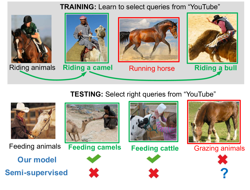
Figure 1: Our model uses a set of annotated data to learn a policy for how to label data for new, unseen classes. This enables learning domain-specific knowledge and how to select diverse exemplars while avoiding semantic drift. For example, it can learn from training data that human motion cues are important for actions involving animals (e.g. “riding animals”) while animal appearance is not. This knowledge can be applied at test time to label noisy data for new classes such as “feeding animals”, while traditional semi-supervised methods would label based on visual similarity.

A promising approach is to leverage noisy data from web queries. Training models for new classes using the data returned by web queries has been proposed as an alternative to expensive manual annotation [7, 8, 19, 28]. Methods for automated labeling of new classes include traditional semi-supervised learning approaches [14, 33, 34] as well as webly-supervised approaches [7, 8, 19]. However, these methods typically rely on iterative hand-tuned data labeling policies. This makes it difficult to dynamically manage the risk trade-off between exemplar diversity and semantic drift. Going further, as a result these methods typically cannot learn domain-specific knowledge. For example, when learning an action recognition model from a set of videos returned by YouTube queries, videos prominently featuring humans are more likely to be positives while those without are more likely to be noise; this intuition is difficult to manually quantify and encode. Even more, when learning an animal-related action such as “feeding animals”, videos containing the action with different animals are likely to be useful positives even though their visual appearance may be different (Fig. 1). Such diverse class-conditional data selection policies are impossible to manually encode. This intuition inspires our work on learning data selection policies for noisy web search results.

Our key insight is that good data labeling policies can be learned from existing manually annotated datasets. Intuitively, a good policy labels noisy data in a way where a classifier trained on the labels would achieve high classification accuracy on a manually annotated held-out set. Although data labeling is a non-differentiable action, this can be naturally achieved in a reinforcement learning setting, where actions correspond to labeling of examples and the reward is the effect on downstream classifier accuracy.

Concretely, we introduce a joint formulation of a Q-learning agent [29] and a class recognition model. In contrast to related webly-supervised approaches [7, 19], the data collection and classifier training steps are not disjoint but rather integrated into a single unified framework. The agent selects web search examples to label as positives, which are then used to train the recognition model. A significant challenge is the choice of the state representation, and we introduce a novel representation based on the distribution of classifier scores output by the recognition model. At training time, the model uses a dataset of labeled training classes to learn a data labeling policy, and at test time the model can use this policy to label noisy web data for new unseen classes.

In summary, our main contribution is a principled formulation for learning how to label noisy web data, using a reinforcement learning framework. To enable this, we also introduce a novel state representation in terms of the classifier score distributions from a jointly trained recognition model. We demonstrate our approach first in the controlled setting of MNIST, then on the large-scale Sports-1M video benchmark [16]. Finally, we show that our method can be used for labeling newly emerging and fine-grained categories where annotated data is scarce.

2 Related work

The difficulty of building large-scale annotated datasets has inspired methods such as [5, 7, 6, 12, 19, 8, 28, 21] which attempts to learn visual (or text [4]) models from noisy web-search results. Such methods usually focus on iteratively gathering examples and using them to improve the visual classifier. Often specific constraints or hand-tuned rules are used for data collection, and successive iterations can cause the model to deviate from the initial concept. We overcome these limitations by automatically learning robust data collection policies resulting in accurate classifiers.

The task of semi-supervised learning also works with limited annotated examples. Popular approaches like transductive SVM [14], label spreading [33] and label propagation [34] induce labels for unannotated examples to explain their distribution. Recent approaches [17, 20, 24, 25, 26, 30] learn an embedding space which captures this distribution. However, these methods do not learn domain-specific knowledge which can help in pruning noisy examples or understanding the multiple subcategories within a class. In contrast, our learned policies adjust for such biases in web-examples of a specific domain.

Approaches like co-segmentation [2, 15], multiple instance learning [1] and zero-shot learning [11, 23, 27, 31] do incorporate domain-specific knowledge. However, unlike our method they do not utilize the large amount of web-search data available for test classes.

Our setup is similar in spirit to meta-learning [3, 10], which attempts to identify both the correct learning algorithm and the parameters required for high accuracy. However, we target a unique goal of building a good dataset for a given class from a large set of noisy web-search examples.

Our key insight is that we can learn policies to directly optimize our goal of choosing a positive set (nondifferentiable actions) leading to an accurate visual classifier, by formulating it in a reinforcement learning setup. We leverage recent advances that enable the use of deep neural networks as function approximators in deep Q-learning [22], and which has shown successful performance in learning policies for game-playing [22], large-scale control problems [9], and simple algorithms [32].

3 Method

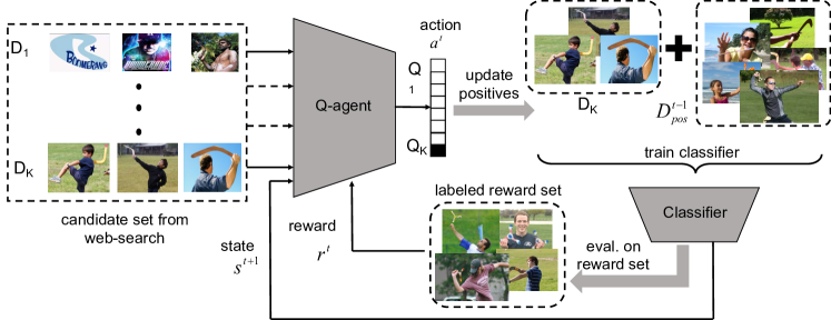
Figure 2: Overview of our model. We learn a classifier for a given visual concept using a candidate set of examples obtained from web search. At each time step $t$ we use the Q-learning agent to select examples, e.g., $D_{K}$, to add to our existing set of positive examples $D_{pos}^{t-1}$. The examples are then used to train a visual classifier. The classifier both updates the agent’s state $s^{t+1}$ and provides a reward $r^{t}$. At test time the trained agent can be used to automatically select positive examples from web search results for any new visual concept.

The goal of our method is to automatically learn an accurate classifier of a visual concept directly from noisy web search results. We refer to these noisy search results as the candidate set $D_{cand}=\{D_{1},\dots,D_{K}\}$, and wish to select a good subset of positives from $D_{cand}$. Such weakly supervised data typically contains diverse subclasses, and the key challenge is to capture this diversity without succumbing to semantic drift. These properties are difficult to objectively quantify. Hence, we want a model which can learn them from existing labeled datasets. One way to achieve this is through an iterative strategy for positive selection, where the model is aware of the positives chosen so far, so that it can promote diversity in future selections. On the other hand, it also needs to avoid semantic drift by being aware of the remaining candidates and learning to estimate long-term change in classifier accuracy. This can be elegantly achieved through a Q-learning formulation.

Hence, our model consists of two components as shown in Fig. 2: (1) a classifier model trained using selected positive examples from the candidate set, and (2) a Q-learning agent which repeatedly selects the positives from the candidate set to train the classifier model.

Note that the visual classes used for training and testing our method are disjoint. For every visual class used during training, in addition to the candidate set, we are also provided a reward set, which is a set of examples annotated with the presence or absence of the target class. The reward set is used to evaluate our model’s ability to produce a good classifier from the candidate set. At test time, we are given just the candidate set for new visual classes.

3.1 Classifier model

The classifier model corresponds to the current visual class considered during a data collection episode and is trained simultaneously with the agent’s data collection policy. At the beginning of an episode, the classifier is seeded with a small set of $S$ positive examples $D_{seed}=\{x_{1},...,x_{S}\}$, as well as a set of negative examples $D_{neg}=\{x_{1},...,x_{N}\}$. In the case of a video search-engine, we assume that the top few retrieved examples are of high enough quality to serve as the seed positives. A random collection of videos from multiple unrelated searches are used to construct the negative set. At each time step $t$, the Q-learning agent makes a selection $a_{t}$ corresponding to examples $D_{a_{t}}$ to be removed from the candidate set $D_{cand}$ and added to the positive training set. The classifier is then trained to distinguish between $D_{pos}=\{D_{seed}\cup D_{a_{1}}\cup...\cup D_{a_{t}}\}$ and $D_{neg}$. The classifier is treated as a black box by the agent; in our experiments, we use a multi-layer perceptron.

3.2 Q-learning agent

The core of our model is a Q-learning agent. Each episode observed by the agent corresponds to data collection for a specific class. At each timestep $t$, the agent observes the current state $s_{t}$, and selects an action $a_{t}$ from a discrete set of actions $\mathcal{A}=\{1,...,K\}$. The action updates the classifier as in Sec. 3.1, and the agent receives a reward $r_{t}$ and the next state observation $s_{t+1}$. The agent’s goal at each timestep is to choose the action that maximizes the future discounted reward $R_{t}=\sum_{t^{\prime}=t}^{T}\gamma^{t^{\prime}-t}r_{t^{\prime}}$, where an episode terminates at time $T$ and $\gamma$ is the discount factor.

There are several key decisions: (1) How to encode the current state of the agent? (2) How to translate this state to a Q-value which can inform the agent’s action? (3) How to formulate a reward function that incentivizes the agent to select optimal examples from the candidate set?

State representation. Our insight in formulating the state representation is that in order to improve the visual classifier, the best examples to use may not be the ones that are the strongest positives according to the current classifier. Instead, it may be better to add some examples with diversity that increase entropy in the positive set. However, too much diversity will cause semantic drift. In order to reason about this, the agent needs to fully understand the distribution of data in the previously selected positive examples $D_{pos}$, in the negative set $D_{neg}$, and in the remaining noisy set $D_{cand}$.

We therefore formulate the agent’s state using the distribution of the classifier scores. Concretely, the state representation is $s=\{H_{pos},H_{neg},\{H_{D_{1}},...,H_{D_{K}}\},P\}$ where $H_{pos},H_{neg},\{H_{D_{1}},...,H_{D_{K}}\}$ are histograms of classifier scores for the positive set, the negative set, and each candidate subset, respectively. $P$ is the proportion of desired number of positives already obtained. The histograms capture the diversity and “prototypicality” of each set (Fig. 4).

Q-network. The agent takes an action $a_{t}$ at time $t$ using a policy $a_{t}=\max_{a}Q(s_{t},a)$, where $s_{t}$ is the state representation above. The Q-value $Q(s_{t},a)$ is determined by a neural network as illustrated in Fig. 3. Concretely, $\alpha_{a}=\phi\left(H_{pos},H_{neg},H_{D_{a}};\theta\right)$ where $\phi(.)$ is a multi-layer perceptron. We use $Q(s,a)=\text{softmax}(\alpha_{a};\tau)$ where $\tau$ is a temperature parameter and helped performance in practice.

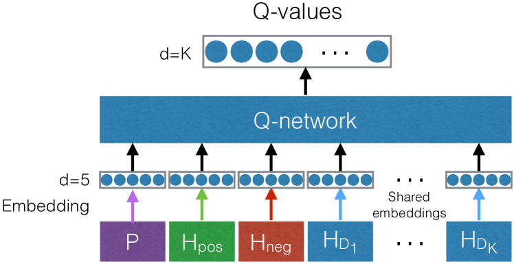
Figure 3: The Q-network, which at each time-step chooses a subset of examples from $D_{1},\dots,D_{K}$. The state representation is $s=\{H_{pos},H_{neg},\{H_{D_{1}},...,H_{D_{K}}\},P\}$ where $H_{pos},H_{neg},\{H_{D_{1}},...,H_{D_{K}}\}$ are histograms of classifier scores for the positive set, the negative set, and each candidate subset. $P$ is the proportion of desired number of positives already obtained.

Generally correct and similar	Generally correct and dissimilar
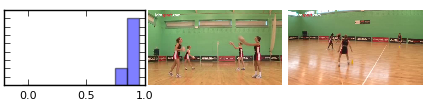
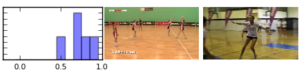
Generally incorrect and similar	Generally incorrect and dissimilar

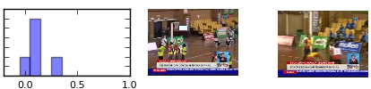
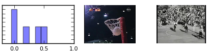
Figure 4: Histograms of classifiers scores for several query buckets with different characteristics, for an example class “Netball”. Example videos from each query are also shown. Buckets with correct vs. incorrect videos have high vs. low scores, while appearance diversity is reflected in histogram peakiness.

Reward function. The agent is incentivized to select the optimal examples from $D_{cand}$ for training a good classifier. We capture this intuition by setting the reward at time $t$ to be the change in the classifier’s accuracy after updating its positive set with the newly chosen examples $D_{a_{t}}$. Accuracy is computed on the held-out annotated data $D_{reward}$. This reward is only available during training.

3.3 Training and testing

We train the agent using Q-learning [29], a standard reinforcement learning algorithm that can be used to learn policies for an agent interacting with an environment. In our case the environment is the visual classifier model. Each episode during training corresponds to a specific visual class, where the agent selects the positive examples of the class from a collection of web-search videos.

The Q-network parameters $\theta$ are learned by optimizing:

$$\small{L_{i}(\theta_{i})}=\small{\mathbb{E}_{s,a}\left[\left(V(\theta_{i-1})-Q(s,a;\theta_{i})\right)^{2}\right],}\vspace{-2pt}$$ (1)

where $i$ is an iteration of optimization and

$$\small{V(\theta_{i-1})}=\small{\mathbb{E}_{s^{\prime}}\left[r+\gamma\max_{a^{\prime}}Q(s^{\prime},a^{\prime};\theta_{i-1})|s,a\right].}\vspace{-2pt}$$ (2)

We optimize it using stochastic gradient descent and experience replay, with random minibatches of past experience $(s_{t},a_{t},r_{t},s_{t+1})$ sampled for training.

The agent is trained to learn data collection policies which can generalize to unseen visual classes. At test time, the agent and the classifier are again run simultaneously on $D_{cand}$ for a new class, but without access to any labeled examples $D_{reward}$. The agent selects videos using the learned greedy policy: $a_{t}=\max_{a}Q(s_{t},a;\theta)$.

4 Experiments

We evaluate our method in three settings: (1) Noisy MNIST digit classification, where we add noise and diversity to MNIST [18] to study our method in a controlled setting, (2) challenging Sports-1M [16] action classification for videos in the wild, and (3) newly emerging and fine-grained classes where annotated data is scarce.

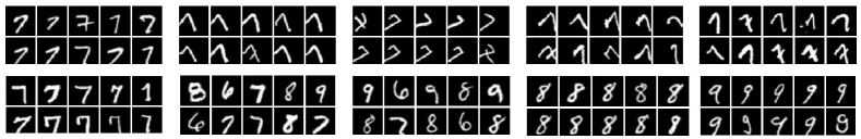
Figure 5: Ten sample query subsets in Noisy MNIST for the digit 7. Top row. Different translation and rotation transformations. Bottom row. The two leftmost queries have different amounts of noise, the center one is a mixture bucket, and the rightmost two are different digits.

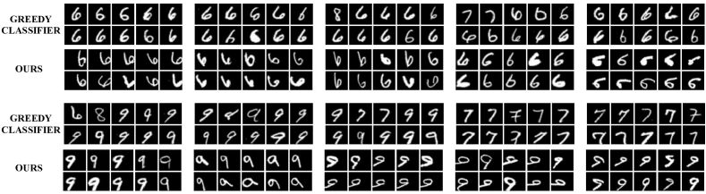
Figure 6: Positive query subsets selected using our method versus the greedy classifier baseline. Subsets chosen by each method are shown from left to right. Top example. The greedy classifier chooses queries with very similar content that would not be useful additional positives, whereas our model chooses diverse queries representing different subconcepts of translation and rotation. Bottom example. The greedy classifier chooses subsets for the positive digit 9 that include increasingly more noise, and eventually chooses a subset with similar-looking 7s that causes it to begin selecting digit 7 subsets instead. In contrast, our model learns policies that are robust to semantic drift.

Setup. We evaluate our model on test classes unseen during training. For every test class, the model selects positive examples from $D_{cand}$ and uses them to train a 1-vs-all classifier. We report the mean average precision (mAP) of this classifier on a manually annotated test set. We consider three scenarios, where the maximum number of positive examples chosen from $D_{cand}$ is limited to $60$, $80$ and $100$ respectively. This allows us to measure performance trade-offs at different budgets. Classifiers are initialized with $D_{seed}$ containing the first 10 web-search results.

Baselines. We compare our model with multiple baselines:

1. Seed. Support vector machine (SVM) learned only from the positive $D_{seed}$.

2. Label propagation. Semi-supervised model from [34] used in an inductive setting to learn from the test $D_{cand}$ and classify the labeled test set.

3. Label spreading. Semi-supervised model from [33] in an inductive setting.

4. TSVM. Transductive support vector machine from [14], which learns a classifier from $D_{cand}$ of test class, and cross-validated using $D_{reward}$.

5. Greedy classifier. An iterative model similar in spirit to [7, 19] that alternates between greedily selecting queries with the highest-scoring contents according to a classifier, and updating the classifier with the newly labeled examples. We use the same classifier model as in our method. On Sports-1M we compare with two additional variants: Greedy-Clustering, which explicitly achieves diversity by clustering labeled positives and ensuring all clusters are represented in new selections; and Greedy-KL which balances diversity and drift by selecting queries whose classifier score distribution most closely achieves a ratio of 0.6 (determined through cross-validation) for KL-divergence with the classifier score distribution of $D_{pos}$ vs. of $D_{neg}$.

Digit	Budget	Seed	Label prop.	Label spread.	TSVM	Greedy	Ours
	60	42.6	37.9	41.1	39.5	43.1	60.9
6	80	42.6	40.8	45.6	44.4	43.2	61.3
	100	42.6	42.2	46.7	46.2	42.4	71.4
	60	48.4	51.1	48.6	46.1	49.7	55.1
7	80	48.4	48.8	48.5	42.6	48.5	57.6
	100	48.4	48.1	46.6	39.7	47.4	55.7
	60	39.1	35.0	35.2	41.2	38.3	56.2
8	80	39.1	40.0	34.1	39.6	39.6	55.6
	100	39.1	42.0	30.2	40.8	38.0	55.5
	60	37.9	37.5	36.5	41.4	52.4	52.4
9	80	37.9	37.9	37.4	38.9	53.5	53.5
	100	37.9	38.0	37.6	39.5	55.7	55.7
	60	42.0	40.4	40.3	42.1	43.4	56.1
All	80	42.0	41.9	41.4	41.4	43.4	57.0
	100	42.0	42.6	40.3	41.5	42.3	59.5

Table 1: AP on Noisy MNIST, with budgets of 60, 80 and 100 corresponding to the numbers of positives selected from $D_{cand}$.

Implementation Details. Our Q-network maps 10-d input histograms in the state representation to a common embedding space of 5 dimensions, with a further hidden layer of 64 units on top. Each episode begins with a seed set of 10 labeled examples, and at training time the network chooses a maximum of 100 total labeled examples needed to train a classifier. The classifier model is a 3-layer multi-layer perceptron with 256 units in each hidden layer, on top of 1000-d ResNet [13] features extracted and then pooled from 10 uniformly sampled frames per video for Sports1M, and on top of raw 784-d pixels for Noisy MNIST. Training consists of 500 episodes for Sports1M, and 200 episodes for Noisy MNIST. The Q-network is trained using experience replay, with mini-batch size 64 and base learning rate $0.01$. A learning update for the agent is taken every 4 iterations, and the target network is softly updated every iteration. A temperature of $\tau=100$ was used in the Q-network.

4.1 Noisy MNIST digit classification

We first evaluate our model in a simulation environment on MNIST digit classification [18], where we can introduce noise and subconcept diversity in a controlled manner. The policies for digit selection are learned from the images of six digits $0-5$ and tested on the other four digits $6-9$.

Setup. For every digit class, example images are randomly split into two sets $S_{c}$ and $S_{r}$ of $500$ images each. The $D_{cand}$ set is constructed using $S_{c}$ by simulating both the sub-concept variation and the noise present in web search results. Concretely, the $S_{c}$ examples are further split into $10$ different query subsets, each containing $5$ sets of $10$ images each. Controlled noise is then added to each query subset: either a specific transformation of the digit (translation and/or rotation), noise from mixed digits, or a different digit. Examples of query subsets for $D_{cand}$ for the digit $7$ are shown in Fig. 5. The $D_{reward}$ set for a digit is constructed from $S_{r}$ by applying translation and/or rotation similar to $D_{cand}$, combined with $1000$ negative images sampled from other digits.

Training. Policies were learned on the $D_{cand}$ set of the training digits to optimize classifier accuracy on the annotated $D_{reward}$ examples. Each episode during training requires the model to pick the best $10$ query subsets from $100$ randomly sampled query subsets of the corresponding candidate set. $D_{neg}$ is constructed by randomly sampling $500$ negative examples of other digits. The model parameters were selected by 3-fold cross validation on training digits.

Testing. The Q-network is used to select a set of $60$, $80$ or $100$ examples from the $D_{cand}$ set of the test digits. The classifier is trained with the selected positives and a set of negatives sampled from $D_{cand}$ of other digits. The same $D_{cand}$ examples are used by all baseline methods as well. Classifier accuracy is evaluated on the annotated test set.

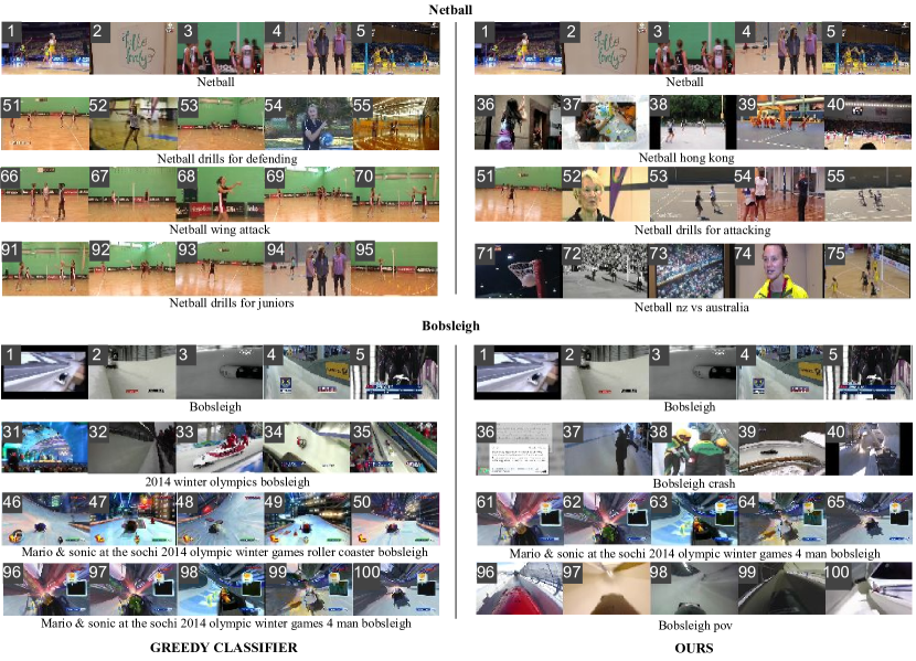
Figure 7: Comparison of positive query subsets selected using our method versus the greedy classifier baseline, for two Sports-1M test classes. Rather than show all 100 selected videos, we highlight interesting differences and show the remaining in Appendix. Each row shows a selected query subset (query phrase and corresponding 5 videos), with the numerical position of the selection out of 100. The first row shows seed videos. Top example. The greedy classifier chooses many similar-looking examples, while our method learns that examples of the action in different environments are useful positives. Bottom example. The greedy classifier drifts from bobsleigh to video games, while our method is robust to semantic drift and selects useful subcategories of bobsleigh videos such as crashes and pov.

Results. Table 1 shows quantitative results from our method compared to the baselines, at varying quantities of positive examples chosen by the methods. Our method outperforms all other baselines at all levels by at least $12.7\%$ mAP. Interestingly, as more positive examples are collected (from 60 to 100), baselines typically improve only slightly or even drop in accuracy, whereas our model consistently improves. Traditional semi-supervised methods such as TSVM, label propagation and spreading are designed to select examples similar to the seed set and thus are unable to cope with the large subclass variations.

Qualitative comparison of our method with the strongest greedy classifier baseline is shown in Fig. 6. It illustrates two major pitfalls of greedy methods: (1) in the first example of the digit 6, the greedy classifier selects images overly similar to the seed-set, to the point of including noise, and (2) in the second example of the digit 9, it gets carried away by semantic drift. Our method is more robust, opting for a diverse selection of subconcepts. It is able to learn that rotations and translations are useful positives for the domain of digits. Interestingly, it tends to gradually expand its understanding of subconcepts, selecting subtle transformations first before more extreme ones. This flexibility to trade-off variety with intra-class similarity allows our model to outperform other methods.

4.2 Sports-1M action recognition

Method	Budget-60	Budget-80	Budget-100
Seed	64.3	64.3	64.3
Label propagation	65.4	65.4	67.2
Label spreading	65.4	66.6	67.3
TSVM	71.6	72.7	73.6
Greedy	71.7	73.8	74.8
Greedy-clustering	72.3	73.2	74.3
Greedy-KL	74.1	74.7	74.7
Ours	75.4	76.2	77.0

Table 2: mAP on Sports-1M with different budgets for the number of selected positive examples.

We evaluate our method in a real-world setting where we want to classify the $487$ human actions in the Sports-1M video dataset [16]. Collecting high-quality video examples for human actions can be very laborious and expensive. Hence, we wish to learn classifiers using only the videos returned by a web search engine without the need for human annotation. The classifiers are trained on noisy examples from YouTube and tested on Sports-1M test videos with ground-truth annotations. We remove any overlapping videos between Sports-1M and YouTube search results to avoid mixing of training and test data. Throughout this section, we ignore the Sports-1M training videos.

We use $300$ classes for training, $105$ classes for testing and the remaining classes for validation, and note that this task is fundamentally different from standard 487-way Sports-1M classification. There is no intersection between the training, testing and validation classes.

Setup. The videos returned by YouTube query search were used to construct the candidate sets for both training and test classes. We constructed $30$ different query expansions for each class using the YouTube query suggestion feature. The top $30$ videos returned from each query were then split into $6$ different pages of 5 videos each. $20$ queries are sampled for each episode during training, resulting in candidate sets of $600$ videos per action class split into $120$ different subsets. The annotated Sports-1M videos of the training classes serve as reward sets used to train the Q-network. Sports-1M videos of test classes are used for evaluation.

Training. In each training episode, the Q-network policies select $20$ subsets ($100$ videos) from the $120$ different query splits of the candidate-set. At each iteration of the episode, the selected positive examples are combined with $500$ random examples from other classes to update the classifier.

Testing and validation. The model parameters were chosen by cross-validation on the validation classes. The final policies are used to select positive examples of test classes from the corresponding YouTube search results. These videos are used to train separate 1-vs-all classifiers for each test class. Each classifier is then evaluated on the annotated positive examples of the corresponding class and $1000$ negative examples sampled from videos of other classes.

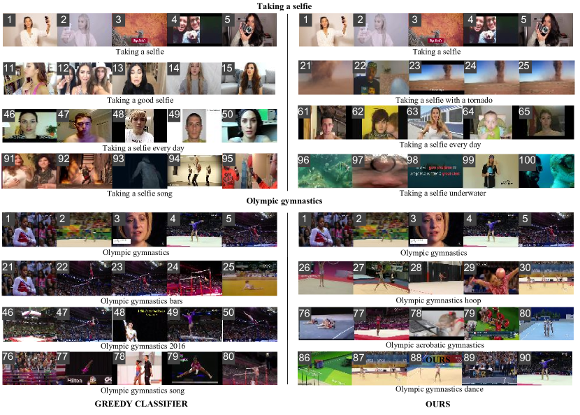
Figure 8: Comparison of positive query subsets selected using our method versus the greedy classifier baseline, for two long-tail classes. See Fig. 7 caption for figure format. Top example. The greedy classifier selects many similar-looking examples of taking a selfie, while our method learns domain-specific knowledge that positives in different environments are more useful, e.g. with a tornado or underwater. Bottom example. The greedy classifier selects similar examples of gymnastics, whereas our method selects visually distinct subcategories.

Results. Table 2 compares our model with baselines. Our model outperforms at all budgets, and at Budget-100 by $2.2\%$ mAP. The margin over the Greedy baseline is higher at smaller budgets, indicating that our model more quickly selects the best positive examples. While Greedy-clustering and Greedy-KL improve over Greedy at small budgets, they perform worse at Budget-100. This illustrates that while using heuristics to explicitly balance diversity and drift can help early on, it is hard to ultimately avoid noise.

Fig. 7 shows positive examples selected by our method compared to the greedy classifier. In the top example of netball, the greedy classifier is overly conservative and selects positives very similar to existing positives, which does not improve classifier accuracy. On the other hand, our model learns domain-specific knowledge that examples of the target action in visually different environments are useful. In the bottom example of bobsleigh, the greedy classifier suffers from the opposite problem: after the classifier selects some queries containing video games, it drifts to queries with more and more video games. In contrast, our model is more robust and returns to clean bobsleigh videos with minimal drift. Furthermore, it selects different subcategories of bobsleigh videos: crash videos, and pov videos, which are useful for training a classifier.

4.3 Long-tail action labeling

We show examples of the policy we learned for Sports-1M on new action classes for which annotated data does not exist in Fig. 8. We compare our learned policy vs. the greedy classifier, for a recent societal-concept: “Taking a selfie”, and a fine-grained class: “Olympic gymnastics”.

The videos selected in Fig. 8 for “Taking a selfie” show that the policy again utilizes domain-specific knowledge that an action in different environments is useful for positive examples: e.g. in front of a volcano, and underwater, even though these have diverse visual appearance. In contrast, the greedy classifier tends to select videos that look very similar to the seed videos. The videos selected for “Olympic gymnastics” demonstrate that the policy selects visually different subcategories: gymnastics with hoops, and gymnastics with acrobatics.

Table 3 measures the diversity and correctness of our model versus the greedy model. Query recall is the number of correct queries which contributed to the selected positives. The correct queries were manually annotated. Our model selects positives from more queries promoting higher diversity. Similarly, our model also avoids noisy examples as seen from video recall: the number of true-positive videos included in the 100 videos selected by each model.

	Query recall		Video recall
Class	Greedy	Ours	Greedy	Ours
Taking a selfie	6/16	9/16	75%	90%
Olympic gymnastics	7/18	10/18	76%	82%

Table 3: Query and video recall of positive videos for two long-tail classes, for our method vs. the greedy classifier. Our method has higher recall of true-positive queries and videos, showing that it selects diverse subconcepts while avoiding semantic drift.

5 Conclusion

In conclusion, we have introduced a principled, reinforcement learning-based formulation for learning how to label noisy web data. We show that our method is able to learn domain-specific knowledge, and label data for new classes in a way that achieves diversity while avoiding semantic drift. We demonstrate our method first in the controlled setting of MNIST, then on large-scale Sports-1M, and finally on newly emerging and fine-grained classes.

References

- [1] S. Andrews, I. Tsochantaridis, and T. Hofmann. Svms for multiple-instance learning. In NIPS, 2002.
- [2] D. Batra, A. Kowdle, D. Parikh, J. Luo, and T. Chen. iCoseg: Interactive co-segmentation with intelligent scribble guidance. In CVPR, 2010.
- [3] P. Brazdil, C. G. Carrier, C. Soares, and R. Vilalta. Metalearning: applications to data mining. Springer Science & Business Media, 2008.
- [4] A. Carlson, J. Betteridge, B. Kisiel, B. Settles, E. R. Hruschka Jr, and T. M. Mitchell. Toward an architecture for never-ending language learning. In AAAI, volume 5, page 3, 2010.
- [5] X. Chen and A. Gupta. Webly supervised learning of convolutional networks. In ICCV, 2015.
- [6] X. Chen and A. Gupta. Webly supervised learning of convolutional networks. In Proceedings of the IEEE International Conference on Computer Vision, pages 1431–1439, 2015.
- [7] X. Chen, A. Shrivastava, and A. Gupta. NEIL: Extracting visual knowledge from web data. In ICCV, 2013.
- [8] S. K. Divvala, A. Farhadi, and C. Guestrin. Learning everything about anything: Webly-supervised visual concept learning. In CVPR, 2014.
- [9] G. Dulac-Arnold, R. Evans, P. Sunehag, and B. Coppin. Reinforcement learning in large discrete action spaces. arXiv preprint arXiv:1512.07679, 2015.
- [10] M. Feurer, A. Klein, K. Eggensperger, J. Springenberg, M. Blum, and F. Hutter. Efficient and robust automated machine learning. In NIPS, 2015.
- [11] A. Frome, G. Corrado, et al. Devise: A deep visual-semantic embedding model. In NIPS, 2013.
- [12] C. Gan, C. Sun, L. Duan, and B. Gong. Webly-supervised video recognition by mutually voting for relevant web images and web video frames. In European Conference on Computer Vision, pages 849–866. Springer, 2016.
- [13] K. He, X. Zhang, S. Ren, and J. Sun. Deep residual learning for image recognition. CoRR:1512.03385, 2015.
- [14] T. Joachims. Transductive inference for text classification using support vector machines. In ICML, 1999.
- [15] A. Joulin, F. Bach, and J. Ponce. Discriminative clustering for image co-segmentation. In CVPR, 2010.
- [16] A. Karpathy, G. Toderici, S. Shetty, T. Leung, R. Sukthankar, and L. Fei-Fei. Large-scale video classification with convolutional neural networks. In CVPR, 2014.
- [17] D. Kingma, D. Rezende, S. Mohamed, and M. Welling. Semi-supervised learning with deep generative models. In NIPS, 2014.
- [18] Y. LeCun, L. Bottou, Y. Bengio, and P. Haffner. Gradient-based learning applied to document recognition. Proceedings of the IEEE, 86:2278–2324, 1998.
- [19] L.-J. Li and L. Fei-Fei. OPTIMOL: automatic online picture collection via incremental model learning. IJCV, 88(2):147–168, 2010.
- [20] X. Li, Y. Guo, and D. Schuurmans. Semi-supervised zero-shot classification with label representation learning. In Proceedings of the IEEE International Conference on Computer Vision, pages 4211–4219, 2015.
- [21] J. Liang, L. Jiang, D. Meng, and A. Hauptmann. Learning to detect concepts from webly-labeled video data. In Joint Conference on Artificial Intelligence (IJCAI), 2016.
- [22] V. Mnih, K. Kavukcuoglu, D. Silver, A. A. Rusu, J. Veness, M. G. Bellemare, et al. Human-level control through deep reinforcement learning. Nature, 518(7540):529–533, 2015.
- [23] M. Palatucci, D. Pomerleau, G. E. Hinton, and T. M. Mitchell. Zero-shot learning with semantic output codes. In Advances in neural information processing systems, pages 1410–1418, 2009.
- [24] N. Pitelis, C. Russell, and L. Agapito. Semi-supervised learning using an unsupervised atlas. In Machine Learning and Knowledge Discovery in Databases, pages 565–580. Springer, 2014.
- [25] M. Ranzato and M. Szummer. Semi-supervised learning of compact document representations with deep networks. In ICML, 2008.
- [26] S. Rifai, Y. N. Dauphin, P. Vincent, Y. Bengio, and X. Muller. The manifold tangent classifier. In NIPS, 2011.
- [27] M. Rohrbach, M. Stark, and B. Schiele. Evaluating knowledge transfer and zero-shot learning in a large-scale setting. In CVPR, 2011.
- [28] F. Schroff, A. Criminisi, and A. Zisserman. Harvesting image databases from the web. TPAMI, 2011.
- [29] C. J. Watkins and P. Dayan. Q-learning. Machine learning, 8(3-4):279–292, 1992.
- [30] J. Weston, F. Ratle, H. Mobahi, and R. Collobert. Deep learning via semi-supervised embedding. In Neural Networks: Tricks of the Trade, pages 639–655. Springer, 2012.
- [31] X. Xu, T. M. Hospedales, and S. Gong. Multi-task zero-shot action recognition with prioritised data augmentation. In European Conference on Computer Vision, pages 343–359. Springer, 2016.
- [32] W. Zaremba, T. Mikolov, A. Joulin, and R. Fergus. Learning simple algorithms from examples. CoRR:1511.07275, 2015.
- [33] D. Zhou, O. Bousquet, T. N. Lal, J. Weston, and B. Schölkopf. Learning with local and global consistency. NIPS, 2004.
- [34] X. Zhu and Z. Ghahramani. Learning from labeled and unlabeled data with label propagation. In ICML, 2002.