A New Randomized Block-Coordinate Primal-Dual Proximal Algorithm for Distributed Optimization

Abstract

This paper proposes TriPD, a new primal-dual algorithm for minimizing the sum of a Lipschitz-differentiable convex function and two possibly nonsmooth convex functions, one of which is composed with a linear mapping. We devise a randomized block-coordinate version of the algorithm which converges under the same stepsize conditions as the full algorithm. It is shown that both the original as well as the block-coordinate scheme feature linear convergence rate when the functions involved are either piecewise linear-quadratic, or when they satisfy a certain quadratic growth condition (which is weaker than strong convexity). Moreover, we apply the developed algorithms to the problem of multi-agent optimization on a graph, thus obtaining novel synchronous and asynchronous distributed methods. The proposed algorithms are fully distributed in the sense that the updates and the stepsizes of each agent only depend on local information. In fact, no prior global coordination is required. Finally, we showcase an application of our algorithm in distributed formation control.

I Introduction

In this paper we consider the optimization problem

$$\underset{x\in{{\rm I\mathchoice{}{}{}{}R}}^{n}}{\operatorname*{minimize\ }}\ {f}({x})+{g}({x})+{{h}}({L}{x}),$$ (1)

where $L$ is a linear mapping, $h$ and $g$ are proper, closed, convex functions (possibly nonsmooth), and $f$ is convex, continuously differentiable with Lipschitz-continuous gradient. We further assume that the proximal mappings associated with $h$ and $g$ are efficiently computable [1]. This setup is quite general and captures a wide range of applications in signal processing, machine learning and control.

In problem (1), it is typically assumed that the gradient of the smooth term $f$ is $\beta_{f}$-Lipschitz for some nonnegative constant $\beta_{f}$. We consider Lipschitz continuity of $\nabla f$ with respect to $\|\cdot\|_{Q}$ with $Q\succ 0$ in place of the canonical norm (cf. (3)). This is because in many applications of practical interest, a scalar Lipschitz constant fails to accurately capture the Lipschitz continuity of $\nabla f$. A prominent example lies in distributed optimization, where $f$ is separable, i.e., $f(x)=\sum_{i=1}^{m}f_{i}(x_{i})$. In this case, the metric $Q$ is taken block-diagonal with blocks containing the Lipschitz constants of the $\nabla f_{i}$’s. Notice that in such settings considering a scalar Lipschitz constant results in using the largest of the Lipschitz constants, which leads to conservative stepsize selection and consequently slower convergence rates.

The main contributions of the paper are elaborated upon in four separate sections below.

I-A A New Primal-Dual Algorithm

In this work a new primal-dual algorithm, TriPD (Alg. 1), is introduced for solving (1). The algorithm consists of two proximal evaluations (corresponding to the two nonsmooth terms $g$ and $h$), one gradient evaluation (for the smooth term $f$), and one correction step (cf. algorithm 1). We adopt the general Lipschitz continuity assumption (3) in our convergence analysis, which is essential for avoiding conservative stepsize conditions that depend on the global scalar Lipschitz constant.

In Section II, it is shown that the sequence generated by TriPD (Alg. 1) is $S$-Fejér monotone (with respect to the set of primal-dual solutions), where $S$ is a block diagonal positive definite matrix. This key property is exploited in Section III to develop a block-coordinate version of the algorithm with a general randomized activation scheme.

The connections of our method to other related primal-dual algorithms in the literature are discussed in Section II-A. Most notably, we recap the Vũ-Condat scheme [2, 3], a popular algorithm used for solving the structured optimization problem (1) (convergence of this method was established independently by Vũ [2] and Condat [3], by casting it in the form of the forward-backward splitting). In the analysis of [2, 3], a scalar constant is used to capture the Lipschitz continuity of the gradient of $f$, thus resulting in potentially smaller stepsizes (and slower convergence in practice). In [4], the authors assume the more general Lipschitz continuity property (3) by using a preconditioned variable metric forward-backward iteration. Nevertheless, the stepsize matrix is restricted to be proportional to $Q^{-1}$. In Section II-A, we show how the analysis technique for the new primal-dual algorithm can be used to recover the Vũ-Condat algorithm with general stepsize matrices, and highlight that this line of analysis leads to less restrictive sufficient conditions on the selected stepsizes compared to [2, 3, 4]. More importantly, it is shown that unlike TriPD (Alg. 1), the Vũ-Condat generated sequence is $S$-Fejér monotone, where $S$ is not diagonal. As we discuss in the next subsection, this constitutes the main difficulty in devising a randomized version of the Vũ-Condat algorithm.

I-B Randomized Block-Coordinate Algorithm

Block-coordinate (BC) minimization is a simple approach for tackling large-scale optimization problems. At each iteration, a subset of the coordinates is updated while others are held fixed. Randomized BC algorithms are of particular interest, and can be divided into two main categories:

Type a) comprises algorithms in which only one coordinate is randomly activated and updated at each iteration. The BC versions of gradient [5] and proximal gradient methods [6] belong in this category. A distinctive attribute of the aforementioned algorithms is the fact that the stepsizes are selected to be inversely proportional to the coordinate-wise Lipschitz constant of the smooth term rather than the global one. This results in applying larger stepsizes in directions with smaller Lipschitz constant, and therefore leads to faster convergence.

Type b) contains methods where more than one coordinate may be randomly activated and simultaneously updated [7, 8]. Note that this class may also capture the single active coordinate (type a) as a special case. The convergence condition for this class of BC algorithms is typically the same as in the full algorithm. In [7, 8] random BC is applied to $\alpha$-averaged operators by establishing stochastic Fejér monotonicity, while [8] also considers quasi-nonexpansive operators. In [9, 7] the authors obtain randomized BC algorithms based on the primal-dual scheme of Vũ and Condat; the main drawback is that, just as in the full version of these algorithms, the use of conservative stepsize conditions leads to slower convergence in practice.

The BC version of TriPD (Alg. 1) falls into the second class, i.e., it allows for a general randomized activation scheme (cf. algorithm 2). The proposed scheme converges under the same stepsize conditions as the full algorithm. As a consequence, in view of the characterization of Lipschitz continuity of $\nabla f$ in (3), when $f$ is separable, i.e., $f(x)=\sum_{i=1}^{m}f_{i}(x_{i})$, our approach leads to algorithms that depend on the local Lipschitz constants (of $\nabla f_{i}$’s) rather than the global constant, thus assimilating the benefits of both categories. Notice that when $f$ is separable, the coordinate-wise Lipschitz continuity assumption of [5, 6, 10] is equivalent to (3) with $\beta_{f}=1$ and $Q=\operatorname{blkdiag}(\beta_{1}I_{n_{1}},\ldots,\beta_{m}I_{n_{m}})$, where $m$ denotes the number of coordinate blocks, $n_{i}$ denotes the dimension of the $i$-th coordinate block, and $\beta_{i}$ denotes the Lipschitz constant of $f_{i}$. In the general setting, [5, Lem. 2] can be invoked to establish the connection between the metric $Q$ and the coordinate-wise Lipschitz assumption. However, in many cases (most notably the separable case) this lemma is conservative.

As mentioned in the prequel, in Section II-A the Vũ-Condat algorithm is recovered using the same analysis that leads to our proposed primal-dual algorithm. It is therefore natural to consider adapting the approach of Section III so as to devise a block-coordinate variant of the the Vũ-Condat algorithm. However, this is not possible given that the Vũ-Condat generated sequence is $S$-Fejér monotone, where $S$ is not diagonal (cf. (20)), while the proof of Theorem III.1 relies heavily on the diagonal structure of $S$. This presents a distinctive merit of our proposed algorithm over the current state-of-the-art for solving problem (1).

In [10], the authors propose a randomized BC version of the Vũ-Condat scheme. Their analysis does not require the cost functions to be separable and utilizes a different Lyapunov function for establishing convergence. Notice that the block-coordinate scheme of [10] updates a single coordinate at every iteration (i.e., it is a type a) algorithm) as opposed to the more general random sweeping of the coordinates. Additionally, in the case of $f$ being separable, our proposed method (cf. algorithm 2) assigns a block stepsize that is inversely proportional to $\tfrac{\beta_{i}}{2}$ (where $\beta_{i}$ denotes the Lipschitz constant for $f_{i}$), in place of ${\beta_{i}}$ required by [10, Assum. 2.1(e)]: larger stepsizes are typically associated with faster convergence in primal-dual proximal algorithms.

I-C Linear Convergence

A third contribution of the paper is establishing linear convergence for the full algorithm under an additional metric subregularity condition for the monotone operator pertaining to the primal-dual optimality conditions (cf. Thm. IV.5). For the BC version, the linear rate is established under a slightly stronger condition (cf. Thm. IV.6). We further explicate the required condition in terms of the objective functions, with two special cases of prevalent interest: a) when $f$, $g$ and $h$ satisfy a quadratic growth condition (cf. Lem. IV.2) (which is much weaker than strong convexity) or b) when $f$, $g$ and $h$ are piecewise linear-quadratic (cf. Lem. IV.4), a common scenario in many applications such as LPs, QPs, SVM and fitting problems for a wide range of regularization functions; e.g. $\ell_{1}$ norm, elastic nets, Huber loss and many more.

Last but not least, it is shown that the monotone operator defining the primal-dual optimality conditions is metrically subregular if and only if the residual mapping (the operator that maps $z^{k}$ to $z^{k}-z^{k+1}$) is metrically subregular (cf. Lem. IV.7). This connection enables the use of Lemmas IV.2 and IV.4 to establish linear convergence for a large class of algorithms based on conditions for the cost functions.

I-D Distributed Optimization

As an important application, we consider a distributed structured optimization problem over a network of agents. In this context, each agent has its own private cost function of the form (1), while the communication among agents is captured by an undirected graph $\mathcal{G}=(\mathcal{V},\mathcal{E})$:

$$\underset{{x}_{1},\ldots,x_{m}}{\operatorname*{minimize\ }} \quad\sum_{i=1}^{m}f_{i}(x_{i})+g_{i}(x_{i})+h_{i}{\mathopen{}\left(L_{i}x_{i}\right)\mathclose{}}$$

$$\operatorname*{subject\ to\ } \quad A_{ij}x_{i}+A_{ji}x_{j}=b_{(i,j)}\qquad(i,j)\in\mathcal{E}.$$

We use $(i,j)$ to denote the unordered pair of agents $i$, $j$, and $ij$ to denote the ordered pair. The goal is to solve the global optimization problem through local exchange of information. Notice that the linear constraints on the edges of the graph prescribe relations between neighboring agents’ variables. This type of edge constraints was also considered in [11]. It is worthwhile noting that for the special case of two agents $i=1,2$, with $f_{i},h_{i}\equiv 0$, one recovers the setup for the celebrated alternating direction method of multipliers (ADMM) algorithm. Another special case of particular interest is consensus optimization, when $A_{ij}=I$, $A_{ji}=-I$ and $b_{(i,j)}=0$. A primal-dual algorithm for consensus optimization was introduced in [12] for the case of $f_{i}\equiv 0$, where a transformation was used to replace the edge variables with node variables.

This multi-agent optimization problem arises in many contexts such as sensor networks, power systems, transportation networks, robotics, water networks, distributed data-sharing, etc. [13, 14, 15]. In most of these applications, there are computation, communication and/or physical limitations on the system that render centralized management infeasible. This motivates the fully distributed synchronous and asynchronous algorithms developed in Section V. Both versions are fully distributed in the sense that not only the iterations are performed locally, but also the stepsizes of each agent are selected based on local information without any prior global coordination (cf. Assumption 6). The asynchronous variant of the algorithm is based on an instance of the randomized block-coordinate algorithm in Section III. The protocol is as follows: at each iteration, a) agents are activated at random, and independently from one another, b) active agents perform local updates, c) they communicate the required updated values to their neighbors and d) return to an idle state.

Notation and Preliminaries

In this section, we introduce notation and definitions used throughout the paper; the interested reader is referred to [16, 17] for more details.

For an extended-real-valued function $f$, we use $\operatorname{dom}f$ to denote its domain. For a set $C$, we denote its relative interior by $\operatorname{ri}C$. The identity matrix is denoted by $I_{n}\in{{\rm I\mathchoice{}{}{}{}R}}^{n\times n}$. For a symmetric positive definite matrix $P\in{{\rm I\mathchoice{}{}{}{}R}}^{n\times n}$, we define the scalar product $\langle x,y\rangle_{P}=\langle x,Py\rangle$ and the induced norm $\|x\|_{P}=\sqrt{\langle x,x\rangle_{P}}$. For simplicity, we use matrix notation for linear mappings when no ambiguity occurs.

An operator (or set-valued mapping) $A:{{\rm I\mathchoice{}{}{}{}R}}^{n}\rightrightarrows{{\rm I\mathchoice{}{}{}{}R}}^{d}$ maps each point $x\in{{\rm I\mathchoice{}{}{}{}R}}^{n}$ to a subset $Ax$ of ${{\rm I\mathchoice{}{}{}{}R}}^{d}$. We denote the domain of $A$ by $\operatorname{dom}A=\{x\in{{\rm I\mathchoice{}{}{}{}R}}^{n}\mid Ax\neq\emptyset\}$, its graph by $\operatorname{gra}A=\{(x,y)\in{{\rm I\mathchoice{}{}{}{}R}}^{n}\times{{\rm I\mathchoice{}{}{}{}R}}^{d}\mid y\in Ax\}$, the set of its zeros by $\operatorname*{zer}A=\{x\in{{\rm I\mathchoice{}{}{}{}R}}^{n}\mid 0\in Ax\}$, and the set of its fixed points by $\operatorname*{fix}A=\{x\mid x\in Ax\}$. The mapping $A$ is called monotone if $\langle x-x^{\prime},y-y^{\prime}\rangle\geq 0$ for all $(x,y),(x^{\prime},y^{\prime})\in\operatorname{gra}A$, and is said to be maximally monotone if its graph is not strictly contained by the graph of another monotone operator. The inverse of $A$ is defined through its graph: $\operatorname{gra}A^{-1}:=\{(y,x)\mid(x,y)\in\operatorname{gra}A\}$. The resolvent of $A$ is defined by $J_{A}:=({\rm Id}+A)^{-1}$, where ${\rm Id}$ denotes the identity operator.

Let $f:{{\rm I\mathchoice{}{}{}{}R}}^{n}\to\overline{{\rm I\mathchoice{}{}{}{}R}}\coloneqq{{\rm I\mathchoice{}{}{}{}R}}\cup\{+\infty\}$ be a proper closed, convex function. Its subdifferential is the operator $\partial f:{{\rm I\mathchoice{}{}{}{}R}}^{n}\rightrightarrows{{\rm I\mathchoice{}{}{}{}R}}^{n}$

$$\partial f(x)=\{y\mid\forall z\in{{\rm I\mathchoice{}{}{}{}R}}^{n},\,f(x)+\langle y,z-x\rangle\leq f(z)\}.$$

It is well-known that the subdifferential of a convex function is maximally monotone. The resolvent of $\partial f$ is called the proximal operator (or proximal mapping), and is single-valued. Let $V$ denote a symmetric positive definite matrix. The proximal mapping of $f$ relative to $\|\cdot\|_{V}$ is uniquely determined by the resolvent of $V^{-1}\partial f$:

$$\operatorname{prox}_{f}^{V}(x) \coloneqq({\rm Id}+V^{-1}\partial f)^{-1}x$$

$$=\operatorname*{\arg\!\min}_{z\in{{\rm I\mathchoice{}{}{}{}R}}^{n}}\{f(z)+\tfrac{1}{2}\|x-z\|_{V}^{2}\}.$$

The Fenchel conjugate of $f$, denoted by $f^{*}$, is defined by $f^{*}(v)\coloneqq\sup_{x\in{{\rm I\mathchoice{}{}{}{}R}}^{n}}\{\langle v,x\rangle-f(x)\}$. The Fenchel-Young inequality states that $\langle x,u\rangle\leq f(x)+f^{*}(u)$ holds for all $x,u\in{{\rm I\mathchoice{}{}{}{}R}}^{n}$; in the special case when $f=\tfrac{1}{2}\|\cdot\|^{2}_{V}$ for some symmetric positive definite matrix $V$, this gives:

$$\langle x,u\rangle\leq\tfrac{1}{2}\|x\|_{V}^{2}+\tfrac{1}{2}\|u\|^{2}_{V^{-1}}.$$ (2)

Let $X$ be a nonempty closed convex set. The indicator of $X$ is defined by $\delta_{X}(x)=0$ if $x\in X$, and $\delta_{X}(x)=\infty$ if $x\notin X$. The distance from $X$ and the projection onto $X$ with respect to $\|\cdot\|_{V}$ are denoted by $d_{V}(\cdot,X)$ and $\mathcal{P}_{X}^{V}(\cdot)$, respectively.

We use $(\Omega,\mathcal{F},\mathbb{P})$ for defining a probability space, where $\Omega$, $\mathcal{F}$ and $\mathbb{P}$ denote the sample space, $\sigma$-algebra, and the probability measure. Moreover, almost surely is abbreviated as a.s.

The sequence $(w^{k})_{k\in{{\rm I\mathchoice{}{}{}{}N}}}$ is said to converge to $w^{\star}$ $Q$-linearly with $Q$-factor $\sigma\in(0,1)$, if there exists $\bar{k}\in{{\rm I\mathchoice{}{}{}{}N}}$ such that for all $k\geq\bar{k}$, $\|w^{k+1}-w^{\star}\|\leq\sigma\|w^{k}-w^{\star}\|$. Furthermore, $(w^{k})_{k\in{{\rm I\mathchoice{}{}{}{}N}}}$ is said to converge to $w^{\star}$ $R$-linearly if there exists a sequence of nonnegative scalars $({v_{k}})_{k\in{{\rm I\mathchoice{}{}{}{}N}}}$ such that $\|w^{k}-w^{\star}\|\leq v^{k}$ and $(v_{k})_{k\in{{\rm I\mathchoice{}{}{}{}N}}}$ converges to zero $Q$-linearly.

II A New Primal-Dual Algorithm

In this section we present a primal-dual algorithm for problem (1). We adhere to the following assumptions throughout sections II, III and IV:

Assumption 1.

1. $g:{{\rm I\mathchoice{}{}{}{}R}}^{n}\to\overline{{\rm I\mathchoice{}{}{}{}R}}$, $h:{{\rm I\mathchoice{}{}{}{}R}}^{r}\to\overline{{\rm I\mathchoice{}{}{}{}R}}$ are proper, closed, convex functions, and $L:{{\rm I\mathchoice{}{}{}{}R}}^{n}\to{{\rm I\mathchoice{}{}{}{}R}}^{r}$ is a linear mapping.

2. ${f}:{{\rm I\mathchoice{}{}{}{}R}}^{n}\to{{\rm I\mathchoice{}{}{}{}R}}$ is convex, continuously differentiable, and for some $\beta_{f}\in[0,\infty)$, $\nabla f$ is $\beta_{f}$-Lipschitz continuous with respect to the metric induced by $Q\succ 0$ , i.e.,

   $$\|\nabla f(x)-\nabla f(y)\|_{Q^{-1}}\!\!\leq\!\beta_{f}\|x-y\|_{Q}\quad\forall x,y\in{{\rm I\mathchoice{}{}{}{}R}}^{n}.$$ (3)

3. The set of solutions to (1) is nonempty. Moreover, there exists $x\in\operatorname{ri}\operatorname{dom}g$ such that $Lx\in\operatorname{ri}\operatorname{dom}h$.

In Item 2), the constant $\beta_{f}\geq 0$ is not absorbed into the metric $Q$ in order to also incorporate the case when $\nabla f$ is a constant (by setting $\beta_{f}=0$).

The dual problem is to

$$\operatorname*{minimize\ }_{u\in{{\rm I\mathchoice{}{}{}{}R}}^{r}}(g+f)^{*}(-L^{\top}u)+h^{*}(u).$$ (4)

With a slight abuse of terminology, we say that $({u}^{\star},{x}^{\star})$ is a primal-dual solution (in place of dual-primal) if ${u}^{\star}$ solves the dual problem (4) and ${x}^{\star}$ solves the primal problem (1). We denote the set of primal-dual solutions by $\mathcal{S}$. Item 3) guarantees that the set of solutions to the dual problem is nonempty and the duality gap is zero [18, Corollary 31.2.1]. Furthermore, the pair $(u^{\star},x^{\star})$ is a primal-dual solution if and only if it satisfies:

$${\mathopen{}\left\{\begin{array}[]{@{}l@{}l@{}}0\in\partial{{h}}^{*}({u})-{L}{x},&\\ 0\in\partial{g}({x})+\nabla{f}(x)+{L}^{\top}{u}.&\end{array}\right.\mathclose{}}$$ (5)

We proceed to present the new primal-dual scheme TriPD (Alg. 1). The motivation behind the name becomes apparent in the sequel after equation (13). The algorithm involves two proximal evaluations (respective to the non-smooth terms $g,h$), and one gradient evaluation (for the Lipschitz-differentiable term $f$). The stepsizes in TriPD (Alg. 1) are chosen so as to satisfy the following assumption:

Assumption 2 (Stepsize selection).

Both the dual stepsize matrix $\Sigma\in{{\rm I\mathchoice{}{}{}{}R}}^{r\times r}$, and the primal stepsize matrix $\Gamma\in{{\rm I\mathchoice{}{}{}{}R}}^{n\times n}$ are symmetric positive definite. In addition, they satisfy:

$$\Gamma^{-1}-{\tfrac{\beta_{f}}{2}}Q-L^{\top}\Sigma L\succ 0.$$ (6)

Selecting scalar primal and dual stepsizes, along with the standard definition of Lipschitz continuity, as is prevalent in the literature [2, 3], can plainly be treated by setting $\Sigma=\sigma I_{r}$, $\Gamma=\gamma I_{n}$, and $Q=I_{n}$, whence from (6) we require that

$$\gamma<\frac{1}{\tfrac{\beta_{f}}{2}+\sigma\|L\|^{2}}.$$

Algorithm 1 Triangularly Preconditioned Primal-Dual algorithm (TriPD)

EndFor

0:  Inputs: $x^{0}\in{{\rm I\mathchoice{}{}{}{}R}}^{n}$, $u^{0}\in{{\rm I\mathchoice{}{}{}{}R}}^{r}$ $k=0,1,\ldots$ $\bar{u}^{k}=\operatorname{prox}_{h^{*}}^{\Sigma^{-1}}(u^{k}+\Sigma L{x^{k}})$ ${x}^{k+1}=\operatorname{prox}_{g}^{\Gamma^{-1}}(x^{k}-\Gamma\nabla f(x^{k})-\Gamma L^{\top}\bar{u}^{k})$ $u^{k+1}=\bar{u}^{k}+\Sigma L({x}^{k+1}-x^{k})$

Remark II.1.

Each iteration of TriPD (Alg. 1) requires one application of $L$ and one of $L^{\top}$ (even though it appears to require two applications of $L$). The reason is that, at iteration $k$, only $L^{\top}\bar{u}^{k}$, $Lx^{k+1}$ need to be evaluated since $L(x^{k+1}-x^{k})=Lx^{k+1}-Lx^{k}$ and $Lx^{k}$ was computed during the previous iteration. ∎

TriPD (Alg. 1) can be compactly written as:

$$z^{k+1}=Tz^{k},$$

where $z^{k}\coloneqq(u^{k},x^{k})$, and the operator $T$ is given by:

$$\bar{u} =\operatorname{prox}_{h^{*}}^{\Sigma^{-1}}(u+\Sigma L{x})$$ (7a)

$$\bar{x} =\operatorname{prox}_{g}^{\Gamma^{-1}}(x-\Gamma\nabla f(x)-\Gamma L^{\top}\bar{u})$$ (7b)

$$Tz =(\bar{u}+\Sigma L(\bar{x}-x),\bar{x}).$$ (7c)

Remark II.2 (Relaxed iterations).

It is also possible to devise a relaxed version of TriPD (Alg. 1) as follows:

$$z^{k+1}=z^{k}+\Lambda(Tz^{k}-z^{k}),$$

where $\Lambda$ is a positive definite matrix and $\Lambda\prec 2I_{n+r}$. For ease of exposition, we present the convergence analysis for the original version (i.e., for $\Lambda=I_{n+r}$). Note that the analysis carries through with minor modifications for relaxed iterations. ∎

For compactness of exposition, we define the following operators:

$$A :({u},{x})\mapsto(\partial{{h}}^{*}({u}),\partial{g}({x})),$$ (8a)

$$M :({u},{x})\mapsto(-{L}x,{L}^{\top}{u}),$$ (8b)

$$C :({u},{x})\mapsto(0,\nabla{f}({x})).$$ (8c)

The optimality condition (5) can then be written in the equivalent form of the monotone inclusion:

$$0\in Az+Mz+Cz\eqqcolon Fz,$$ (9)

where $z=({u},{x})$. Observe that the linear operator $M$ is monotone since it is skew-symmetric, i.e., $M^{\top}=-M$. It is also easy to verify that the operator $A$ is maximally monotone [17, Thm. 21.2 and Prop. 20.23], while operator $C$ is cocoercive, being the gradient of $\tilde{f}(u,x)=f(x)$, and in light of Item 2) and [17, Thm. 18.16].

We further define

$$P=\begin{pmatrix}\Sigma^{-1}&\frac{1}{2}{L}\\ \frac{1}{2}{L}^{\top}&\Gamma^{-1}\end{pmatrix},\quad K=\begin{pmatrix}0&-\tfrac{1}{2}{L}\\ \tfrac{1}{2}{L}^{\top}&0\end{pmatrix},$$ (10)

and set $H=P+K$. It is plain to check that condition (6) implies that the symmetric matrix $P$ is positive definite (by a standard Schur complement argument). In addition, we set

$$S=\operatorname{blkdiag}(\Sigma^{-1},\Gamma^{-1}).$$ (11)

Using these definitions, the operator $T$ defined in (7) can be written as:

$$Tz\coloneqq z+S^{-1}(H+M^{\top})(\bar{z}-z),$$ (12)

where

$$\bar{z}=(H+A)^{-1}(H-M-C)z.$$ (13)

This compact representation simplifies the convergence analysis. A key consideration for choosing $P$ and $K$ as in (10) is to ensure that $H=P+K$ is lower block-triangular. Notice that when $M\equiv 0$, (12) can be viewed as a triangularly preconditioned forward-backward update, followed by a correction step. This motivates the name TriPD: Triangularly Preconditioned Primal-Dual algorithm. Due to the triangular structure of $H$, the backward step $(H+A)^{-1}$ in (13) can be carried out sequentially: an updated dual vector $\bar{u}$ is computed (through proximal mapping) using $(u,x)$ and, subsequently, the primal vector $\bar{x}$ is computed using $\bar{u}$ and $x$, cf. (7). Furthermore, it follows from (12) that this choice makes $H+M^{\top}$ upper block-triangular which, alongside the diagonal structure of $S$, yields the efficiently computable update (7c) in view of:

$$S^{-1}(H+M^{\top})=\begin{pmatrix}I&\Sigma{L}\\ 0&I\end{pmatrix}.$$ (14)

Remark II.3.

The operator in (12) is inspired from [19, Alg. 1], where operators of this form were introduced for devising a splitting method for solving general monotone inclusions of the form in (9). We note, in passing, that the aforementioned algorithm entails an additional dynamic stepsize parameter ($\alpha_{n}$, therein). Although we may also adopt this here, for potentially improving the rate of convergence in practice, we opt not to: the reason is that in the context of multi-agent optimization (that we especially target in this paper) such design choice would require global coordination, that is contradictory to our objective of devising distributed algorithms. As a positive side-effect, the convergence analysis is greatly simplified compared to [19, Sec. 5]. Besides, we use stepsize matrices (in place of scalar stepsizes) in TriPD (Alg. 1) along with the general Lipschitz continuity property (cf. Item 2)) as an essential means for avoiding conservative stepsizes, which is especially important for large-scale distributed optimization. ∎

We proceed by showing that the set of primal-dual solutions coincides with the set of fixed points of $T$, $\operatorname*{fix}T$:

$$\mathcal{S}=\{z\mid 0\in Az+Mz+Cz\}=\operatorname*{fix}T.$$ (15)

To see this note that from (12) and (13) we have:

$$z\in\operatorname*{fix}T\iff z=Tz\iff\bar{z}=z$$

$$\iff (H+A)^{-1}(H-M-C)z=z$$

$$\iff Hz-Mz-Cz\in Hz+Az\iff z\in\mathcal{S},$$

where in the second equivalence we used the fact that $S$ is positive definite and $\langle(H+M^{\top})z,z\rangle\geq\|z\|^{2}_{P}$ for all $z\in{{\rm I\mathchoice{}{}{}{}R}}^{n+r}$ (since $K$ is skew-adjoint and $M$ is monotone).

Next, let us define

$$\tilde{P}\coloneqq\begin{pmatrix}\Sigma^{-1}&-\frac{1}{2}{L}\\ -\frac{1}{2}{L}^{\top}&\Gamma^{-1}-\tfrac{\beta_{f}}{4}Q\end{pmatrix}.$$ (16)

Observe that (from Schur complement) Assumption 2 is necessary and sufficient for $2\tilde{P}-S$ to be symmetric positive definite (cf. to the convergence result in Thm. II.5). In particular, $\tilde{P}$ is positive definite since $S$ is positive definite.

The next lemma establishes the key property of the operator $T$ that is instrumental in our convergence analysis:

Lemma II.4.

Let Assumptions 1 and 2 hold. Consider the operator $T$ in (7) (equivalently (12)). Then for any $z^{\star}\in\mathcal{S}$ and any $z\in{{\rm I\mathchoice{}{}{}{}R}}^{n+r}$ we have

$$\|Tz-{z}\|_{\tilde{P}}^{2}\leq\langle{z}-z^{\star},{z}-Tz\rangle_{S}.$$ (17)

Proof.

See Appendix A. ∎

The next theorem establishes the main convergence result for TriPD (Alg. 1). In specific, it is shown that the generated sequence is $S$-Fejér monotone. We emphasize that the diagonal structure of $S$ is the key property used in developing the block-coordinate version of the algorithm in Section III.

Theorem II.5.

Let Assumptions 1 and 2 hold. Consider the sequence $({z}^{k})_{k\in{{\rm I\mathchoice{}{}{}{}N}}}$ generated by TriPD (Alg. 1). The following Fejér-type inequality holds for all $z^{\star}\in\mathcal{S}$:

$$\|z^{k+1}-z^{\star}\|_{S}^{2}{}\leq{}\|z^{k}-z^{\star}\|_{S}^{2}-\|z^{k+1}-z^{k}\|_{2{\tilde{P}}-S}^{2}.$$ (18)

Consequently, $({z}^{k})_{k\in{{\rm I\mathchoice{}{}{}{}N}}}$ converges to some $z^{\star}\in\mathcal{S}$.

Proof.

See Appendix A. ∎

II-A Related Primal-Dual Algorithms

Recently, the design of primal-dual algorithms for solving problem (1) (possibly with $f\equiv 0$ or $g\equiv 0$) has received a lot of attention in the literature. Most of the existing approaches can be interpreted as applications of one of the three main splittings techniques: forward-backward (FB), Douglas-Rachford (DR), and forward-backward-forward (FBF) splittings [2, 3, 20, 21], while others employ different tools to establish convergence [22, 23].

A unifying analysis for primal-dual algorithms is proposed in [19, Sec. 5], where in place of FBS, DRS, or FBFS, a new three-term splitting, namely asymmetric forward-backward adjoint (AFBA) is used to design primal-dual algorithms. In particular, the algorithms of [21, 20, 22, 2, 3, 23] are recovered (under less restrictive stepsize conditions) and other new primal-dual algorithms are proposed. As discussed in Remark II.3 the AFBA splitting [19, Alg. 1] is the motivation behind the operator $T$ defined in (12). We refer the reader to [19, Sec. 5] and [24] for a detailed discussion on the relation between primal-dual algorithms.

Next we briefly discuss how the celebrated algorithm of Vũ and Condat [3, 2] can be seen as fixed-point iterations of the operator $T$ in (12) for an appropriate selection of $S$, $P$, $K$.

In [3] Condat considers problem (1), while Vũ [2] considers the following variant:

$$\underset{x\in{{\rm I\mathchoice{}{}{}{}R}}^{n}}{\operatorname*{minimize\ }}\ {f}({x})+{g}({x})+(h\mathbin{\scaleobj{0.75}{\square}}l)({L}{x}),$$ (19)

where $l$ is a strongly convex function and $\mathbin{\scaleobj{0.75}{\square}}$ represents the infimal convolution [17]. For this problem, an additional assumption is that the conjugate of $l$ is continuously differentiable, and $\nabla l^{*}$ is $\beta_{l}$-Lipschitz continuous with respect to a metric $G\succ 0$, for some $\beta_{l}\geq 0$, cf. (3). Note that it is possible to derive and analyze a variant of TriPD (Alg. 1) for (19), however, we do not pursue this in this paper and focus on problem (1) for clarity of exposition and length considerations.

One can verify that the operator defining the fixed-point iterations in the Vũ-Condat algorithm is given by (12) with $H=P+K$ and $S$ defined as follows:

$$S=\begin{pmatrix}\Sigma^{-1}&{L}\\ {L}^{\top}&\Gamma^{-1}\end{pmatrix},$$ (20)

$$P=\begin{pmatrix}\Sigma^{-1}&{L}\\ {L}^{\top}&\Gamma^{-1}\end{pmatrix},\quad K=\begin{pmatrix}0&-{L}\\ {L}^{\top}&0\end{pmatrix}.$$

For such selection of $S$, $P$, $K$, it holds that $S^{-1}(H+M^{\top})=I$, whence in proximal form, the operator defined in (12) becomes:

$$\bar{u} =\operatorname{prox}_{h^{*}}^{\Sigma^{-1}}(u-\Sigma\nabla l^{*}(u)+\Sigma L{x})$$

$$\bar{x} =\operatorname{prox}_{g}^{\Gamma^{-1}}(x-\Gamma\nabla f(x)-\Gamma L^{\top}(2\bar{u}-u))$$

$$Tz =(\bar{u},\bar{x}).$$

Observe the non-diagonal structure of $S$ for the Vũ-Condat algorithm in (20), in contrast with the one for TriPD (Alg. 1) in (11). For the sake of comparison with [3, 2] we consider the relaxed iteration $z^{k+1}=z^{k}+\lambda(Tz^{k}-z^{k})$ for some $\lambda\in(0,2)$, in this subsection (which we opted to exclude from TriPD (Alg. 1) solely for the purpose of simplicity).

The analysis in Theorem II.5 can be further used to establish convergence of the Vũ-Condat scheme for problem (19) under the following sufficient conditions (in place of Assumption 2):

$$\Sigma^{-1}-\tfrac{\beta_{l}}{2(2-\lambda)}G\succ 0,$$ (21a)

$$\Gamma^{-1}-\tfrac{\beta_{f}}{2(2-\lambda)}Q-L^{\top}{\mathopen{}\left(\Sigma^{-1}-\tfrac{\beta_{l}}{2(2-\lambda)}G\right)\mathclose{}}^{-1}L\succ 0.$$ (21b)

Notice that when $l=\delta_{\{0\}}$ (i.e., for problem (1)), $l^{*}\equiv 0$ whence $\beta_{l}=0$, and the condition simplifies to:

$$\Gamma^{-1}-\tfrac{\beta_{f}}{2(2-\lambda)}Q-L^{\top}\Sigma L\succ 0.$$

Given the stepsize condition (21) the following Fejér-type inequality holds.

$$\|z^{k+1}-z^{\star}\|_{S}^{2}{}\leq{}\|z^{k}-z^{\star}\|_{S}^{2}-\lambda\|z^{k+1}-z^{k}\|_{2{\hat{P}}-\lambda S}^{2},$$ (22)

with $S$ defined in (20) and $\hat{P}$ given by:

$$\hat{P}\coloneqq\begin{pmatrix}\Sigma^{-1}-\tfrac{\beta_{l}}{4}G&{L}\\ {L}^{\top}&\Gamma^{-1}-\tfrac{\beta_{f}}{4}Q\end{pmatrix}.$$

This generalizes the result in [3, Thm. 3.1], [2, Cor. 4.2] and [19, Prop. 5.1] where $Q=I$ and the stepsizes are assumed to be scalar.

Our main goal here was to demonstrate the non-diagonal structure of $S$ for the Vũ-Condat algorithm. In the sequel, we highlight that our analysis additionally leads to less conservative conditions as compared to [2, 3, 4]. Notice that the proofs in the aforementioned papers are based on casting the algorithm in the form of forward-backward iterations. Consequently, the stepsize condition obtained ensures that the underlying operator is averaged. In contradistinction, the sufficient condition in (21) only ensures that the Fejér-type inequality (22) holds, which is sufficient for convergence. Therefore, even in the case of scalar stepsizes (as in [2, 3]) condition (21) allows for larger stepsizes compared to [2, 3].

In [4, 9] the authors propose a variable metric version of the algorithm with a preconditioning that accounts for the general Lipschitz metric. This is accomplished by fixing the stepsize matrix to be a constant times the inverse of the Lipschitz metric, and obtaining a condition on the constant. Our approach does not assume this restrictive form for the stepsize matrix; even when such a restriction is imposed it allows for larger stepsizes, thus achieving generally faster convergence. As an illustrative example, let us set $\Gamma=\mu Q^{-1}$ and $\Sigma=\nu G^{-1}$ for some $\mu,\nu>0$. For simplicity and without loss of generality, let $\beta_{l}=1$, $\beta_{f}=1$. Then (21) simplifies to:

$$(\mu^{-1}-\tfrac{1}{2(2-\lambda)})(\nu^{-1}-\tfrac{1}{2(2-\lambda)})Q-L^{\top}G^{-1}L\succ 0,$$ (23)

whereas the condition required in [4, 9] is $\lambda\in(0,1]$ and

$${\frac{\delta}{1+\delta}>\frac{\max\{\mu,\nu\}}{2}\;\textrm{with }\;\delta=\tfrac{1}{\sqrt{\nu\mu}}\|G^{-1/2}LQ^{-1/2}\|^{-1}-1.}$$ (24)

It is not difficult to check that condition, (23), is always less restrictive than (24). For instance, let $G^{-1/2}LQ^{-1/2}=I$ and set $\mu=1.5$, then (23) requires that $\nu<\tfrac{1}{6.5}$ whereas (24) necessitates that $\nu<\tfrac{1}{24}$.

III A Randomized Block-Coordinate Algorithm

In this section, we describe a randomized block-coordinate variant of TriPD (Alg. 1) and discuss important special cases pertaining to the randomized coordinate activation mechanism. The convergence analysis is based on establishing stochastic Fejér monotonicity [8] of the generated sequence. In addition, we establish linear convergence of the method under further assumptions in Section IV.

First, let us define a partitioning of the vector of primal-dual variables into $m$ blocks of coordinates. Notice that each block might include a subset of primal or dual variables, or a combination of both. Respectively, let $U_{i}\in{{\rm I\mathchoice{}{}{}{}R}}^{(n+r)\times(n+r)}$, for $i=1,\ldots,m$, be a diagonal matrix with $0$-$1$ diagonal entries that is used to select a subset of the coordinates (selected coordinates correspond to diagonal entries equal to $1$). We call such matrix an activation matrix, as it is used to activate/select a subset of coordinates to update.

Let $\Phi=\{0,1\}^{m}$ denote the set of binary strings of length $m$ (with the elements considered as column vectors of dimension $m$). At the $k$-th iteration, the algorithm draws a $\Phi$-valued random activation vector $\epsilon^{k+1}$ which determines which blocks of coordinates will be updated. The $i$-th element of the vector $\epsilon^{k+1}$ is denoted as $\epsilon_{i}^{k+1}$: the $i$-th block is updated at iteration $k$ if $\epsilon_{i}^{k+1}=1$. Notice that in general multiple blocks of coordinates may be concurrently updated. The conditional expectation ${\operatorname*{\mathbb{E}}}{\mathopen{}\left[\cdot\mid\mathcal{F}_{k}\right]\mathclose{}}$ is abbreviated by ${\operatorname*{\mathbb{E}}}_{k}{\mathopen{}\left[\cdot\right]\mathclose{}}$, where $\mathcal{F}_{k}$ is the filtration generated by $(\epsilon^{1},\ldots,\epsilon^{k})$. The following assumption summarizes the setup of the randomized coordinate selection.

Assumption 3.

1. $\{U_{i}\}_{i=1}^{m}$ are $0$-$1$ diagonal matrices and $\sum_{i=1}^{m}U_{i}=I.$

2. $(\epsilon^{k})_{k\in{{\rm I\mathchoice{}{}{}{}N}}}$ is a sequence of i.i.d. $\Phi$-valued random vectors with

   $$p_{i}\coloneqq\mathbb{P}(\epsilon^{1}_{i}=1)>0\quad i=1,\ldots,m.$$ (25)

3. The stepsize matrices $\Sigma,\Gamma$ are diagonal.

The first condition implies that the activation matrices define a partition of the coordinates, while the second that each partition is activated with a positive probability.

We further define the (diagonal) coordinate activation probability matrix $\Pi$ as follows:

$$\Pi\coloneqq\sum_{i=1}^{m}p_{i}U_{i}.$$ (26)

For $\epsilon=(\epsilon_{1},\ldots,\epsilon_{m})$ we define the operator $\hat{T}^{(\epsilon)}$ by:

$$\hat{T}^{(\epsilon)}z\coloneqq z+\sum_{i=1}^{m}\epsilon_{i}U_{i}(Tz-z),$$

where $T$ was defined in (7) (equivalently (12)). Observe that this is a compact notation for the update of only the selected blocks. The randomized scheme is then written as an iterative application of $\hat{T}^{(\epsilon^{k+1})}$ for $k=0,1,\ldots$ (this operator updates the active blocks of coordinates and leaves the others unchanged, i.e., equal to their previous iterate values). The randomized block-coordinate scheme is summarized below.

Algorithm 2 Block-coordinate TriPD algorithm

EndFor

0:  Inputs: $x^{0}\in{{\rm I\mathchoice{}{}{}{}R}}^{n}$, $u^{0}\in{{\rm I\mathchoice{}{}{}{}R}}^{r}$ $k=0,1,\ldots$ Select $\Phi$-valued r.v. $\epsilon^{k+1}$$z^{k+1}=\hat{T}^{(\epsilon^{k+1})}z^{k}$

We emphasize that the randomized model that we adopt here is capable of capturing many stationary randomized activation mechanisms. To illustrate this, consider the following activation mechanisms (of specific interest in the realm of distributed multi-agent optimization, cf. Section V):

• Multiple coordinate activation: at each iteration, the $j$-th coordinate block is randomly activated with probability $p_{j}>0$ independent of other coordinates blocks. This corresponds to the case that the sample space is equal to $\Phi=\{0,1\}^{m}$. The general distributed algorithm of Section V assumes this mechanism.

• Single coordinate activation: at each iteration, one coordinate block is selected, i.e., the sample space is

  $$\{(1,0,\ldots,0),(0,1,0,\ldots,0)\ldots,(0,\ldots,0,1)\}.$$ (27)

  We assign probability $p_{i}$ to the event $\epsilon_{i}=1$ (and $\epsilon_{j}=0$ for $j\neq i$), whence the probabilities must satisfy $\sum_{i=1}^{m}p_{i}=1$.

The next lemma establishes stochastic Fejér monotonicity for the generated sequence, by directly exploiting the diagonal structure of $S$. The proof technique is adapted from [7, Thm. 3] (see also [25, Thm. 2], [8, Thm. 2.5]), and is based on the Robbins-Siegmund lemma [26].

Theorem III.1.

Let Assumptions 1, 2 and 3 hold. Consider the sequence $({z}^{k})_{k\in{{\rm I\mathchoice{}{}{}{}N}}}$ generated by TriPD-BC (Alg. 2). The following Fejér-type inequality holds for all $z^{\star}\in\mathcal{S}$:

$$\mathbb{E}_{k}{\mathopen{}\left[\|z^{k+1}-z^{\star}\|_{\Pi^{-1}S}^{2}\right]\mathclose{}}{}\leq{} \|z^{k}-z^{\star}\|_{\Pi^{-1}S}^{2}$$

$$-\|Tz^{k}-z^{k}\|_{2\tilde{P}-S}^{2}.$$ (28)

Consequently, $({z}^{k})_{k\in{{\rm I\mathchoice{}{}{}{}N}}}$ converges a.s. to some $z^{\star}\in\mathcal{S}$.

Proof.

See Appendix A. ∎

It is important to emphasize that a naive implementation of TriPD-BC (Alg. 2) (with regards to the partitioning of primal-dual variables) may involve wasteful computations. As an example, consider a BC algorithm in which, at every iteration, either all primal or all dual variables are updated. In such a case, if at iteration $k$ the dual vector is to be updated, both $x^{k+1}$, $u^{k+1}$ are computed (cf. algorithm 1), whereas only $u^{k+1}$ is updated. This phenomenon is common to all primal-dual algorithms, and is due to the fact that the primal and dual updates need to be performed sequentially in the full version of the algorithm. As a consequence, the blocks of coordinates must be partitioned in such a way that computations are not discarded, so that the iteration cost of a BC algorithm is (substantially) smaller than computing the full operator $T$. This choice relies entirely on the structure of the optimization problem under consideration. A canonical example of prominent practical interest is the setting of multi-agent optimization in a network (cf. section V), where $L$ is not diagonal, $f$ and $g$ are separable, and additional coupling between (primal) coordinates is present through $h$, see (32). In this example, the primal and dual coordinates are partitioned in such a way that no computation is discarded (cf. section V for more details).

We proceed with another example where the coordinates may be grouped such that the BC algorithm does not incur any wasteful computations: consider problem (1) with $Lx=\operatorname{blkdiag}(L_{1}x_{1},\ldots,L_{m}x_{m})$, and $g$, $h$ separable functions i.e.,

$$\underset{x\in{{\rm I\mathchoice{}{}{}{}R}}^{n}}{\operatorname*{minimize\ }}\ {f}({x})+\sum_{i=1}^{m}\big{(}g_{i}(x_{i})+h_{i}(L_{i}x_{i})\big{)}.$$

In this problem, the coupling between the (primal) coordinates is carried via function $f$. For each $i=1,\ldots,m$, we can choose $U_{i}$ such that it selects the $i$-th primal-dual coordinate block $(u_{i},x_{i})$. Under such partitioning of coordinates, one may use TriPD-BC (Alg. 2) with any random activation pattern satisfying Assumption 3. For example, for the case of multiple independently activated coordinates, as discussed above, at iteration $k$ the following is performed

$${\mathopen{}\left\{\leavevmode\nobreak\ \!\!\leavevmode\nobreak\ \parbox{433.62pt}{ \lx@algorithmic@beginlist{{\footnotesize 0:}}{ } \State\scalebox{0.75}{\textbullet} each block $(u_{i},x_{i})$ is activated with probability $p_{i}>0$ \State\scalebox{0.75}{\textbullet} for active block(s) $i$ compute: \State$\bar{u}^{k}_{i}=\operatorname{prox}_{\sigma h_{i}^{*}}(u^{k}_{i}+\sigma L_{i}x^{k}_{i})$ \State${x}^{k+1}_{i}=\operatorname{prox}_{\gamma g_{i}}(x^{k}_{i}-\gamma\nabla_{i}f(x^{k})-\gamma L^{\top}_{i}\bar{u}^{k}_{i})$ \State$u^{k+1}_{i}=\bar{u}^{k}_{i}+\sigma L_{i}({x}^{k+1}_{i}-x^{k}_{i})$. \lx@algorithmic@endlist}\right.\mathclose{}}$$

More generally, when $g$ and $h$ are separable in problem (1), and $L$ is such that either each (block) row only has one nonzero element or each (block) column has one nonzero element, then the coordinates can be grouped together in such a way that no wasteful computations occur: in the first case the primal vector $x_{i}$ and all dual vectors $u_{j}$ that are required for its computation are selected by $U_{i}$ (with the role of primal and dual reversed in the second case).

Remark III.2.

Note that in TriPD-BC (Alg. 2) the probabilities $p_{i}$ are taken fixed, i.e., the matrix $\Pi$ is constant throughout the iterations. This is a non-restrictive assumption and can be relaxed by considering iteration-varying probabilities $p_{i}^{k}$ in (25) and modifying TriPD-BC (Alg. 2) by setting:

$$z^{k+1}=z^{k}+\sum_{i=1}^{m}\tfrac{\epsilon_{i}^{k+1}}{mp_{i}^{k+1}}U_{i}(Tz^{k}-z^{k}).$$

Let $\Pi^{k}$ denote the probability matrix defined as in (26) using $p_{i}^{k}$. Then, by arguing as in Theorem III.1, it can be shown that the following stochastic Fejér monotonicity holds for the modified sequence:

$$\mathbb{E}_{k}{\mathopen{}\left[\|z^{k+1}-z^{\star}\|_{S}^{2}\right]\mathclose{}}\leq \|z^{k}-z^{\star}\|_{S}^{2}$$

$$-\|Tz^{k}-z^{k}\|_{\tfrac{2}{m}\tilde{P}-\tfrac{1}{m^{2}}S(\Pi^{k+1})^{-1}}^{2}.$$

∎

IV Linear Convergence

In this section, we establish linear convergence of Algorithms 1 and 2 under additional conditions on the cost functions $f$, $g$ and $h$. To this end, we show that linear convergence is attained if the monotone operator $F=A+M+C$ defining the primal-dual optimality conditions (cf. (9)) is metrically subregular (globally metrically subregular in the case of TriPD-BC (Alg. 2)). A notable consequence of our analysis is the fact that linear convergence is attained when the cost functions either a) belong in the class of piecewise linear-quadratic (PLQ) convex functions or b) when they satisfy a certain quadratic growth condition (which is much weaker than strong convexity). Moreover, notice that in the case of PLQ the solution need not be unique (cf. Thm.s IV.5 and IV.6).

We first recall the notion of metric subregularity [27].

Definition IV.1 (Metric subregularity).

A set-valued mapping $F:{{\rm I\mathchoice{}{}{}{}R}}^{n}\rightrightarrows{{\rm I\mathchoice{}{}{}{}R}}^{d}$ is metrically subregular at $\bar{x}$ for $\bar{y}$ if $(\bar{x},\bar{y})\in\operatorname{gra}F$ and there exists a positive constant $\eta$ together with a neighborhood of subregularity $\mathcal{U}$ of $\bar{x}$ such that

$$d(x,F^{-1}\bar{y})\leq{} \eta d(\bar{y},Fx){\;\;\forall}x\in\mathcal{U}.$$

If the following stronger condition holds

$$\|x-\bar{x}\|\leq{} \eta d(\bar{y},Fx)\;\;\forall x\in\mathcal{U},$$

then $F$ is said to be strongly subregular at $\bar{x}$ for $\bar{y}$.

Moreover, we say that $F$ is globally (strongly) subregular at $\bar{x}$ for $\bar{y}$ if (strong) subregularity holds with $\mathcal{U}={{\rm I\mathchoice{}{}{}{}R}}^{n}$.

We refer the reader to [16, Chap. 9], [27, Chap. 3] and [28, Chap. 2] for further discussion on metric subregularity.

Metric subregularity of the subdifferential operator has been studied thoroughly and is equivalent to the quadratic growth condition [29, 30] defined next. In particular, for a proper closed convex function $f$, the subdifferential $\partial f$ is metrically subregular at $\bar{x}$ for $\bar{y}$ with $(\bar{x},\bar{y})\in\operatorname{gra}\partial f$ if and only if there exists a positive constant $c$ and a neighborhood $\mathcal{U}$ of $\bar{x}$ such that the following growth condition holds [29, Thm. 3.3]:

$$f(x)\geq f(\bar{x})+\langle\bar{y},x-\bar{x}\rangle+cd^{2}(x,(\partial{f})^{-1}(\bar{y}))\quad\forall x\in\mathcal{U}$$

Furthermore, $\partial f$ is strongly subregular at $\bar{x}$ for $\bar{y}$ with $(\bar{x},\bar{y})\in\operatorname{gra}\partial f$, if and only if there exists a positive constant $c$ and a neighborhood $\mathcal{U}$ of $\bar{x}$ such that [29, Thm. 3.5]:

$$f(x)\geq f(\bar{x})+\langle\bar{y},x-\bar{x}\rangle+c\|x-\bar{x}\|^{2}\quad\forall x\in\mathcal{U}$$ (29)

Note that strongly convex functions satisfy (29), but (29) is much weaker than strong convexity, as it is a local condition: it only holds in a neighborhood of $\bar{x}$, and also only for $\bar{y}$.

The lemma below provides a sufficient condition for metric subregularity of the monotone operator $A+M+C$, in terms of strong subregularity of $\nabla f+\partial g$ and $\partial h^{*}$ (equivalently the quadratic growth of $f+g$ and $h^{*}$, cf. (29)) as stated in the following assumption:

Assumption 4 (Strong subregularity of $\nabla f+\partial g$ and $\partial h^{*}$).

There exists $z^{\star}=(u^{\star},x^{\star})\in\mathcal{S}$ satisfying:

1. $\nabla f+\partial g$ is strongly subregular at $x^{\star}$ for $-L^{\top}u^{\star}$,

2. $\partial h^{*}$ is strongly subregular at $u^{\star}$ for $Lx^{\star}$.

We say that $f$, $g$ and $h$ satisfy this assumption globally if the strong subregularity assumption of $\nabla f+\partial g$ and $\partial h^{*}$ both hold globally (cf. Definition IV.1).

In particular, Assumption 4 holds globally if either $f$ or $g$ (or both) are strongly convex and $h$ is continuously differentiable with Lipschitz continuous gradient, i.e., $h^{*}$ is strongly convex.

Lemma IV.2.

Let Assumptions 1 and 4 hold. Then $F=A+M+C$ (cf. (8)) is strongly subregular at ${z}^{\star}$ for $0$. Moreover, if $f$, $g$ and $h$ satisfy Assumption 4 globally, then $F$ is globally strongly subregular at ${z}^{\star}$ for $0$. In both cases the set of primal-dual solutions is a singleton, $\mathcal{S}=\{z^{\star}\}$.

Proof.

See Appendix A. ∎

Our next objective is to show that $A+M+C$ is globally metrically subregular when the functions $f$, $g$ and $h$ are piecewise linear-quadratic (PLQ). Note that this assumption does not imply that the set of solutions $\mathcal{S}$ is a singleton, nevertheless, linear convergence can still be established. Let us recall the definition of PLQ functions [16]:

Definition IV.3 (Piecewise linear-quadratic).

A function $f:{{\rm I\mathchoice{}{}{}{}R}}^{n}\to\overline{{\rm I\mathchoice{}{}{}{}R}}$ is called piecewise linear-quadratic (PLQ) if its domain can be represented as the union of finitely many polyhedral sets, and in each such set $f(x)$ is given by an expression of the form $\frac{1}{2}\langle x,Qx\rangle+\langle d,x\rangle+c$, for some $c\in{{\rm I\mathchoice{}{}{}{}R}}$, $d\in{{\rm I\mathchoice{}{}{}{}R}}^{n}$, and symmetric matrix $Q\in{{\rm I\mathchoice{}{}{}{}R}}^{n\times n}$.

The class of PLQ functions is closed under scalar multiplication, addition, conjugation and Moreau envelope [16]. A wide range of functions used in optimization applications belong to this class, for example: affine functions, quadratic forms, indicators of polyhedral sets, polyhedral norms (e.g., the $\ell_{1}$-norm), and regularizing functions such as elastic net, Huber loss, hinge loss, to name a few.

Lemma IV.4.

Let Assumption 1 hold. In addition, assume that $f$, $g$ and $h$ are piecewise linear-quadratic. Then $F=A+M+C$ (cf. (8)) is metrically subregular with the same constant $\eta$ at any $z$ for any $v$ with $(z,v)\in\operatorname{gra}F$.

Proof.

See Appendix A. ∎

Our main convergence rate results are provided in Theorems IV.5 and IV.6. In this context, Lemmas IV.4 and IV.2 are used to establish sufficient conditions in terms of the cost functions. We omit the proof of Theorem IV.5 for length considerations. The proof is similar to that of Theorem IV.6, the main difference being that in Theorem IV.5 local (as opposed to global) metric subregularity is used: due to the Fejér-type inequality (18), $\bar{z}^{k}$ will eventually be contained in a neighborhood of metric subregularity, where inequality (53) applies.

Theorem IV.5 (Linear convergence of algorithm 1).

Consider TriPD (Alg. 1) under the assumptions of Theorem II.5. Suppose that $F=A+M+C$ is metrically subregular at all $z^{\star}\in\mathcal{S}$ for $0$. Then $(d_{S}({z}^{k},\mathcal{S}))_{k\in{{\rm I\mathchoice{}{}{}{}N}}}$ converges $Q$-linearly to zero, and $(z^{k})_{k\in{\rm{I\!N}}}$ converges $R$-linearly to some $z^{\star}\in\mathcal{S}$.

In particular, the metric subregularity assumption holds and the result follows if either one of the following holds:

1. either $f$, $g$ and $h$ are PLQ,

2. or $f$, $g$ and $h$ satisfy Assumption 4, in which case the solution is unique.

Theorem IV.6 (Linear convergence of algorithm 2).

Consider TriPD-BC (Alg. 2) under the assumptions of Theorem III.1. Suppose that $F=A+M+C$ is globally metrically subregular for $0$ (cf. Def. IV.1), i.e., there exists $\eta>0$ such that

$$d(z,F^{-1}0)\leq\eta d(0,Fz)\quad\forall z\in{{\rm I\mathchoice{}{}{}{}R}}^{n+r}.$$

Then $(\operatorname*{\mathbb{E}}{\mathopen{}\left[d^{2}_{\Pi^{-1}S}({z}^{k},\mathcal{S})\right]\mathclose{}})_{k\in{{\rm I\mathchoice{}{}{}{}N}}}$ converges $Q$-linearly to zero.

The same holds if

1. either $f,g,h$ are PLQ and there exists a compact set $\mathcal{C}$ such that $(z^{k})_{k\in{{\rm I\mathchoice{}{}{}{}N}}}\subseteq\mathcal{C}$ (as is the case if $\operatorname{dom}g$ and $\operatorname{dom}h^{*}$ are compact),

2. or $f$, $g$ and $h$ satisfy Assumption 4 globally, in which case the solution is unique.

Proof.

See Appendix A. ∎

In the recent work [31] the authors establish linear convergence in the framework of non-expansive operators under the assumption that the residual mapping defined as $R={\rm Id}-T$ is metrically subregular. However, such a condition is not easily verifiable in terms of conditions on the cost functions. In the next lemma, we show that $R$ is metrically subregular if and only if the monotone operator $F$ is metrically subregular. This result connects the two assumptions and is interesting in its own right. More importantly, it enables the use of Lemmas IV.2 and IV.4 for establishing linear convergence for a wide array of problems.

Lemma IV.7.

Let Assumptions 1 and 2 hold. Consider the operator $T$ defined in (12) and a point $z^{\star}\in\mathcal{S}$. Then $F=A+M+C$ (cf. (8)) is metrically subregular at $z^{\star}$ for $0$ if and only if the residual mapping $R\coloneqq{\rm Id}-T$ is metrically subregular at $z^{\star}$ for $0$.

Proof.

See Appendix A. ∎

V Distributed Optimization

In this section, we consider a general formulation for multi-agent optimization over a network, and leverage Algorithms 1 and 2 to devise both synchronous and randomized asynchronous distributed primal-dual algorithms. The setting is as follows. We consider an undirected graph $\mathcal{G}=(\mathcal{V},\mathcal{E})$ over a vertex set $\mathcal{V}=\{1,\ldots,m\}$ with edge set $\mathcal{E}\subset{\mathcal{V}\times\mathcal{V}}$. Each vertex is associated with a corresponding agent, which is assumed to have a local memory and computational unit, and can only communicate with its neighbors. We define the neighborhood of agent $i$ by $\mathcal{N}_{i}\coloneqq\{j|(i,j)\in\mathcal{E}\}$. We use the terms vertex, agent, and node interchangeably. The goal is to solve the following global optimization problem in a distributed fashion:

$$\underset{x_{1},\ldots,x_{m}}{\operatorname*{minimize\ }} \quad\sum_{i=1}^{m}f_{i}(x_{i})+g_{i}(x_{i})+h_{i}{\mathopen{}\left(L_{i}x_{i}\right)\mathclose{}}$$ (30a)

$$\operatorname*{subject\ to\ } \quad A_{ij}x_{i}+A_{ji}x_{j}=b_{(i,j)}\qquad(i,j)\in\mathcal{E},$$ (30b)

where $x_{i}\in{{\rm I\mathchoice{}{}{}{}R}}^{n_{i}}$. The cost functions $f_{i}$, $g_{i}$, $h_{i}\circ L_{i}$ are taken private to agent/node $i\in\mathcal{V}$, i.e., our distributed methods operate solely by exchanging local variables among neighboring nodes that are unaware of each other’s objectives. The coupling in the problem is represented through the edge constraints (30b).

Throughout this section the following assumptions hold:

Assumption 5.

For each $i=1,\ldots,m$:

1. For $j\in\mathcal{N}_{i}$, $b_{(i,j)}\in{{\rm I\mathchoice{}{}{}{}R}}^{l_{(i,j)}}$ and $A_{ij}\in{{\rm I\mathchoice{}{}{}{}R}}^{n_{i}}\to{{\rm I\mathchoice{}{}{}{}R}}^{l_{(i,j)}}$ is a linear mapping.

2. $g_{i}:{{\rm I\mathchoice{}{}{}{}R}}^{n_{i}}\to\overline{{\rm I\mathchoice{}{}{}{}R}}$, $h_{i}:{{\rm I\mathchoice{}{}{}{}R}}^{r_{i}}\to\overline{{\rm I\mathchoice{}{}{}{}R}}$ are proper closed convex functions, and $L_{i}:{{\rm I\mathchoice{}{}{}{}R}}^{n_{i}}\to{{\rm I\mathchoice{}{}{}{}R}}^{r_{i}}$ is a linear mapping.

3. $f_{i}:{{\rm I\mathchoice{}{}{}{}R}}^{n_{i}}\to{{\rm I\mathchoice{}{}{}{}R}}$ is convex, continuously differentiable, and for some $\beta_{i}\in[0,\infty)$, $\nabla f_{i}$ is $\beta_{i}$-Lipschitz continuous with respect to the metric $Q_{i}\succ 0$, i.e.,

   $$\|\nabla{f}_{i}(x)-\nabla{f}_{i}(y)\|_{Q_{i}^{-1}}\leq\beta_{i}\|x-y\|_{Q_{i}}\quad x,y\in{{\rm I\mathchoice{}{}{}{}R}}^{n_{i}}.$$

4. The graph $\mathcal{G}$ is connected.

5. The set of solutions of (30) is nonempty. Moreover, there exists $x_{i}\in\operatorname{ri}\operatorname{dom}g_{i}$ such that $L_{i}x_{i}\in\operatorname{ri}\operatorname{dom}h_{i}$, for $i=1,\ldots,m$, and $A_{ij}x_{i}+A_{ji}x_{j}=b_{(i,j)}$ for $(i,j)\in\mathcal{E}$.

Algorithm 3 Synchronous & asynchronous versions of TriPD-Dist algorithm

EndFor

0:  Inputs: $x_{i}^{0}\in{{\rm I\mathchoice{}{}{}{}R}}^{n_{i}}$, $y_{i}^{0}\in{{\rm I\mathchoice{}{}{}{}R}}^{r_{i}}$, for $i=1,\ldots,m$, and $w_{(i,j),i}\in{{\rm I\mathchoice{}{}{}{}R}}^{l_{(i,j)}}$ for $j\in\mathcal{N}_{i}$. $k=0,1,\ldots$

0:   I: Synchronous version for all agents $i=1,\ldots,m$ do II: Asynchronous version Each agent $i=1.\ldots,m$ is activated independently with probability $p_{i}>0$ for all active agents do Local updates:    $\mathclap{{\bar{w}}_{(i,j),i}^{k}}=\tfrac{1}{2}\big{(}{w}_{(i,j),i}^{k}+{w}_{(i,j),j}^{k}\big{)}+\tfrac{\kappa_{(i,j)}}{2}\big{(}A_{ij}x_{i}^{k}+A_{ji}{x}_{j}^{k}-b_{(i,j)}\big{)},\quad\forall j\in\mathcal{N}_{i}$   $\mathclap{\bar{{y}}_{i}^{k}}=\operatorname{prox}_{\sigma_{i}{{h}_{i}}^{\star}}\big{(}{y}_{i}^{k}+\sigma_{i}{L}_{i}{x}_{i}^{k}\big{)}$    $\mathclap{{{x}}_{i}^{k+1}}=\operatorname{prox}_{\tau_{i}{g}_{i}}\big{(}{x}_{i}^{k}-\tau_{i}{L}_{i}^{\top}\bar{{y}}_{i}^{k}-\tau_{i}\sum_{j\in\mathcal{N}_{i}}A_{ij}^{\top}\bar{w}_{(i,j),i}^{k}-\tau_{i}\nabla{f_{i}}({x_{i}^{k}})\big{)}$    $\mathclap{y_{i}^{k+1}}=\bar{{y}}_{i}^{k}+\sigma_{i}{L}_{i}({x}_{i}^{k+1}-x_{i}^{k})$    $\mathclap{w_{(i,j),i}^{k+1}}=\bar{w}_{(i,j),i}^{k}+\kappa_{(i,j)}{A_{ij}}({x}_{i}^{k+1}-x_{i}^{k}),\quad\forall j\in\mathcal{N}_{i}$ Transmission of information:    Send $A_{ij}x_{i}^{k+1}$, $w_{(i,j),i}^{k+1}$ to agent $j$, $\forall j\in\mathcal{N}_{i}$

Each agent $i\in\mathcal{V}$ maintains its own local primal variable $x_{i}\in{{\rm I\mathchoice{}{}{}{}R}}^{n_{i}}$ and dual variables $y_{i}\in{{\rm I\mathchoice{}{}{}{}R}}^{r_{i}}$, and $w_{(i,j),i}\in{{\rm I\mathchoice{}{}{}{}R}}^{l_{(i,j)}}$ (for each $j\in\mathcal{N}_{i}$), where the former is related to the linear mapping $L_{i}$, and the latter is the local dual variable of agent $i$ corresponding to the edge-constraint (30b). It is important to note that the updates in TriPD-Dist (Alg. 3) are performed locally through communication with neighbors: the only information that agent $i$ shares with its neighbor $j\in\mathcal{N}_{i}$ is the quantity $A_{ij}x_{i}$, along with edge variable $w_{(i,j),i}$, while all other variables are kept private.

The proposed distributed protocol features both a synchronous as well as an asynchronous implementation. In the synchronous version, at every iteration, all the agents update their variables. In the randomized asynchronous implementation, only a subset of randomly activated agents perform updates, at each iteration, and they do so using their local variables as well as information previously communicated to them by their neighbors. After an update is performed, in both cases, updated values are communicated to neighboring agents. Notice that the asynchronous scheme corresponds to the case of multiple coordinate blocks activation in TriPD-BC (Alg. 2). Other activation schemes can also be considered, and our convergence analysis plainly carries over; notably, the single agent activation which corresponds to the asynchronous model of [32, 33, 34] in which agents are assumed to ‘wake-up’ based on independent exponentially distributed tick-down timers.

Furthermore, in TriPD-Dist (Alg. 3) each agent $i$ keeps positive local stepsizes $\sigma_{i}$, $\tau_{i}$ and ${\mathopen{}\left(\kappa_{(i,j)}\right)\mathclose{}}_{j\in\mathcal{N}_{i}}$. The edge weights/stepsizes $\kappa_{(i,j)}$ may alternatively be interpreted as inherent parameters of the communication graph. For example, they may be used to capture edge’s ‘fidelity,’ e.g., the channel quality in a communication link. The stepsizes are assumed to satisfy the following local assumption that is sufficient for the convergence of the algorithm (cf. Thm.s V.1 and V.2).

Assumption 6 (Stepsizes of TriPD-Dist (Alg. 3)).

1. (node stepsizes) Each agent $i$ keeps two positive stepsizes $\sigma_{i}$, $\tau_{i}$.

2. (edge stepsizes) A positive stepsize $\kappa_{(i,j)}$ is associated with edge $(i,j)\in\mathcal{E}$, and is shared between agents $i$, $j$.

3. (convergence condition) The stepsizes satisfy the following local condition

   $$\tau_{i}<\frac{1}{\tfrac{\beta_{i}\|Q_{i}\|}{2}+\|\sigma_{i}L_{i}^{\top}L_{i}+\sum_{j\in\mathcal{N}_{i}}\kappa_{(i,j)}A_{ij}^{\top}A_{ij}\|}.$$

According to Item 3) the stepsizes $\tau_{i},\sigma_{i}$ for each agent only depend on the local parameters $\beta_{i}$, $\|Q_{i}\|$, the edge weights, $\kappa_{(i,j)}$ and the linear mappings $L_{i}$, and $A_{ij}$, which are all known to agent $i$; therefore the stepsizes can be selected locally, in a decentralized fashion.

We proceed by casting the multi-agent optimization problem (30) in the form of the structured optimization problem (1). In doing so, we describe how TriPD-Dist (Alg. 3) is derived as an instance of Algorithms 1 and 2.

Define the linear operator

$$N_{(i,j)}:\mathsf{x}\mapsto(A_{ij}x_{{i}},A_{ji}x_{{j}}),$$

and $\mathsf{N}\in{{\rm I\mathchoice{}{}{}{}R}}^{2\sum_{(i,j)\in\mathcal{E}}l_{(i,j)}\times\sum_{i=1}^{m}n_{i}}$ by stacking $N_{(i,j)}$:

$$\mathsf{N}:\mathsf{x}\mapsto(N_{(i,j)}\mathsf{x})_{{(i,j)}\in\mathcal{E}}.$$

Its transpose is given by:

$$\mathsf{N}^{\top}:(w_{(i,j)})_{(i,j)\in\mathcal{E}}\mapsto\tilde{\mathsf{x}}=\sum_{(i,j)\in\mathcal{E}}N^{\top}_{(i,j)}w_{(i,j)},$$

with $\tilde{x}_{i}=\sum_{j\in\mathcal{N}_{i}}A^{\top}_{ij}w_{(i,j),i}$. We have set $w_{(i,j)}=(w_{(i,j),i},w_{(i,j),j})$, i.e., we consider two dual variables (of dimension $l_{(i,j)}$) for each edge constraint, where $w_{(i,j),i}$ is maintained by agent $i$ and $w_{(i,j),j}$ by agent $j$.

Consider the set

$$C_{(i,j)}=\{(z_{1},z_{2})\in{{\rm I\mathchoice{}{}{}{}R}}^{l_{(i,j)}}\times{{\rm I\mathchoice{}{}{}{}R}}^{l_{(i,j)}}\mid z_{1}+z_{2}=b_{(i,j)}\}.$$

Then problem (30) can then be re-written as:

$$\operatorname*{minimize\ }\sum_{i=1}^{m} f_{i}(x_{i})+g_{i}(x_{i})+h_{i}{\mathopen{}\left(L_{i}x_{i}\right)\mathclose{}}$$

$$+ \sum_{(i,j)\in\mathcal{E}}\delta_{C_{(i,j)}}(N_{(i,j)}\mathsf{x})$$ (31)

Let $C=\bigtimes_{(i,j)\in\mathcal{E}}C_{(i,j)}$, $L=\operatorname{blkdiag}(L_{1},\ldots,L_{m})$, and $\mathsf{L}\mathsf{x}=(L\mathsf{x},\mathsf{N}\mathsf{x})=:(\mathsf{\tilde{y}},\mathsf{\tilde{w}})\in{{\rm I\mathchoice{}{}{}{}R}}^{n_{d}}$ with $n_{d}=2\sum_{(i,j)\in\mathcal{E}}l_{(i,j)}+\sum_{i=1}^{m}r_{i}$, and rewrite (31) in the following compact form:

$$\operatorname*{minimize\ }\ \mathsf{f}(\mathsf{x})+\mathsf{g}(\mathsf{x})+\tilde{\mathsf{h}}(\mathsf{L}\mathsf{x}),$$ (32)

where $\mathsf{f}(\mathsf{x})=\sum_{i=1}^{m}{f}_{i}(x_{i})$, $\mathsf{g}(\mathsf{x})=\sum_{i=1}^{m}{g}_{i}(x_{i})$, $\tilde{\mathsf{h}}(\mathsf{\tilde{y}},\mathsf{\tilde{w}})=\mathsf{h}(\mathsf{\tilde{y}})+\delta_{C}(\mathsf{\tilde{w}})$, $\mathsf{h}(\mathsf{\tilde{y}})=\sum_{i=1}^{m}{h}_{i}(\tilde{y}_{i})$.

In what follows, $\mathcal{S}$ refers to the set of primal-dual solutions of (32). As in Section II, the primal-dual optimality conditions can be written in the form of monotone inclusion (9) with

$$A: (\mathsf{y},\mathsf{w},\mathsf{x})\mapsto(\partial\mathsf{h}^{*}(\mathsf{y}),\partial\delta^{*}_{C}(\mathsf{w}),\partial\mathsf{g}(\mathsf{x})),$$

$$M: (\mathsf{y},\mathsf{w},\mathsf{x})\mapsto(-L\mathsf{x},-\mathsf{N}\mathsf{x},{L}^{\top}{\mathsf{y}}+\mathsf{N}^{\top}\mathsf{w}),$$

$$C: (\mathsf{y},\mathsf{w},\mathsf{x})\mapsto(0,0,\nabla{}\mathsf{f}(\mathsf{x})),$$

where $\mathsf{{u}}=(\mathsf{{y}},\mathsf{{w}})$ represents the dual vector.

We define the edge weight matrix as follows

$$W=\operatorname{blkdiag}{\mathopen{}\left((\kappa_{(i,j)}I_{2l_{(i,j)}})_{(i,j)\in\mathcal{E}}\right)\mathclose{}},$$

where the weights $\kappa_{(i,j)}$ are repeated twice (for each of the two neighboring agents). Furthermore, we set

$$\Sigma =\operatorname{blkdiag}(\sigma_{1}I_{r_{1}},\ldots,\sigma_{m}I_{r_{m}},W),$$

$$\Gamma =\operatorname{blkdiag}(\tau_{1}I_{n_{1}},\ldots,\tau_{m}I_{n_{m}}),$$

$$Q =\operatorname{blkdiag}(\beta_{1}Q_{1},\ldots,\beta_{m}Q_{m}).$$

Since $\operatorname{prox}_{\tilde{\mathsf{h}}^{\star}}(\mathsf{y},\mathsf{w})=(\operatorname{prox}_{{\mathsf{h}}^{\star}}(\mathsf{y}),\mathsf{w}-\mathcal{P}_{C}(\mathsf{w}))$ (using $\operatorname{prox}_{\delta_{C}}(\cdot)=\mathcal{P}_{C}(\cdot)$ along with Moreau decomposition [17, Thm. 14.3]) the proximal updates of TriPD (Alg. 1), cf. (7), become:

$$\bar{{y}}_{i} =\operatorname{prox}_{\sigma_{i}{{h}_{i}}^{\star}}({y}_{i}+\sigma_{i}{L}_{i}{x}_{i}),$$

$$\bar{{w}}_{(i,j)}\!\! ={w}_{(i,j)}\!+\!\kappa_{(i,j)}({N}_{(i,j)}\mathsf{x}-\mathcal{P}_{C_{(i,j)}}\!\!(\kappa_{(i,j)}^{-1}{w}_{(i,j)}+{N}_{(i,j)}\mathsf{x})),$$

$$\bar{{x}}_{i} =\operatorname{prox}_{\tau_{i}{g}_{i}}\!\!\!({x}_{i}-\tau_{i}{L}_{i}^{\top}\bar{{y}_{i}}-\tau_{i}(\mathsf{N}^{\top}\bar{\mathsf{w}})_{i}-\tau_{i}\nabla{f}({x_{i}})).$$

Note that for $w_{1},w_{2}\in{{\rm I\mathchoice{}{}{}{}R}}^{l_{(i,j)}}$ the projection onto $C_{(i,j)}$ is

$$\mathcal{P}_{C_{(i,j)}}(w_{1},w_{2})=\frac{1}{2}{\mathopen{}\left(w_{1}-w_{2}+b_{(i,j)},-w_{1}+w_{2}+b_{(i,j)}\right)\mathclose{}}.$$

By assigning to agent $i$ the primal coordinate $x_{i}$ and dual coordinate $y_{i}$ and $w_{(i,j),i}$ for all $j\in\mathcal{N}_{i}$, TriPD-Dist (Alg. 3) is obtained. Note that this assignment entails non-overlapping sets of coordinates, i.e., Item 1) is satisfied.

The convergence results of TriPD-Dist (Alg. 3) are provided separately for the synchronous and asynchronous schemes in the next two theorems, along with a sufficient condition for linear convergence. The proofs follow directly from Theorems IV.5 and IV.6.

Theorem V.1 (Convergence of Algorithm 3-I).

Let Assumptions 5 and 6 hold. The sequence $(\mathsf{z}^{k})_{k\in{{\rm I\mathchoice{}{}{}{}N}}}=(\mathsf{y}^{k},\mathsf{w}^{k},\mathsf{x}^{k})_{k\in{{\rm I\mathchoice{}{}{}{}N}}}$ generated by Algorithm 3-I converges to some $z^{\star}\in\mathcal{S}$. Furthermore, if $f_{i}$, $g_{i}$ and $h_{i}$, $i=1,\ldots,m$ are PLQ, then $(d_{S}(\mathsf{z}^{k},\mathcal{S}))_{k\in{{\rm I\mathchoice{}{}{}{}N}}}$ converges $Q$-linearly to zero, and $(\mathsf{z}^{k})_{k\in{{\rm I\mathchoice{}{}{}{}N}}}$ converges $R$-linearly to $z^{\star}\in\mathcal{S}$.

Theorem V.2 (Convergence of Algorithm 3-II).

Let Assumptions 5 and 6 hold. The sequence $(\mathsf{z}^{k})_{k\in{{\rm I\mathchoice{}{}{}{}N}}}=(\mathsf{y}^{k},\mathsf{w}^{k},\mathsf{x}^{k})_{k\in{{\rm I\mathchoice{}{}{}{}N}}}$ generated by Algorithm 3-II converges almost surely to some $z^{\star}\in\mathcal{S}$. Furthermore, if $f_{i}$, $g_{i}$ and $h_{i}$, $i=1,\ldots,m$ are PLQ and $(\mathsf{z}^{k})_{k\in{{\rm I\mathchoice{}{}{}{}N}}}\subseteq\mathcal{C}$ where $\mathcal{C}$ is a compact set, then $(\operatorname*{\mathbb{E}}{\mathopen{}\left[d^{2}_{\Pi^{-1}S}(\mathsf{z}^{k},\mathcal{S})\right]\mathclose{}})_{k\in{{\rm I\mathchoice{}{}{}{}N}}}$ converges $Q$-linearly to zero.

VI Application: Formation Control

In this section we consider the problem of formation control of a group of robots [15, 35], where each robot/agent has its own local dynamics and cost function and the goal is to achieve a specific formation by communicating only with neighboring agents.

For simplicity of visualization we consider a $2$D problem. Each subsystem (corresponding to a robot) has four states $x_{i}=(p_{x_{i}},p_{y_{i}},v_{x_{i}},v_{y_{i}})$, where $(p_{x_{i}},p_{y_{i}})$ and $(v_{x_{i}},v_{y_{i}})$ denote the position and the velocity vectors, respectively. The input for each system is given by $u_{i}=(v^{u}_{x_{i}},v^{u}_{y_{i}})$. The discrete-time LTI model of each system is given by

$$x_{i}(k+1)=\Phi_{i}x_{i}(k)+\Delta_{i}u_{i}(k),\quad k=0,1,\ldots.$$

The state and input transition matrices are as follows

$$\Phi_{i}=\begin{pmatrix}I&0&X_{1}&0\\ 0&I&0&X_{1}\\ 0&0&X_{2}&0\\ 0&0&0&X_{2}\end{pmatrix},\quad\Delta_{i}=\begin{pmatrix}X_{3}&0\\ 0&X_{3}\\ X_{1}&0\\ 0&X_{1}\end{pmatrix},$$

where the parameters are $X_{1}=-t_{d}(e^{-\tfrac{1}{t_{d}}}-1)$, $X_{2}=e^{-\tfrac{1}{t_{d}}}$ and $X_{3}=t_{d}^{2}(e^{-\tfrac{1}{t_{d}}}-1+\tfrac{1}{t_{d}})$ with time constant $t_{d}=5$ (s). This discrete-time model was derived from the continuous-time model of [35] using exact discretization with step length $\Delta T=1$.

Let $N$ denote the horizon length. Consider the stacked state and input vectors $\mathchoice{\text{\boldmath{$\displaystyle x$}}}{\text{\boldmath{$\textstyle x$}}}{\text{\boldmath{$\scriptstyle x$}}}{\text{\boldmath{$\scriptscriptstyle x$}}}_{i}\in{{\rm I\mathchoice{}{}{}{}R}}^{4N},\mathchoice{\text{\boldmath{$\displaystyle u$}}}{\text{\boldmath{$\textstyle u$}}}{\text{\boldmath{$\scriptstyle u$}}}{\text{\boldmath{$\scriptscriptstyle u$}}}_{i}\in{{\rm I\mathchoice{}{}{}{}R}}^{2N}$:

$$\mathchoice{\text{\boldmath{$\displaystyle x$}}}{\text{\boldmath{$\textstyle x$}}}{\text{\boldmath{$\scriptstyle x$}}}{\text{\boldmath{$\scriptscriptstyle x$}}}_{i}\coloneqq(x_{i}(1),\ldots,x_{i}(N)),\;\mathchoice{\text{\boldmath{$\displaystyle u$}}}{\text{\boldmath{$\textstyle u$}}}{\text{\boldmath{$\scriptstyle u$}}}{\text{\boldmath{$\scriptscriptstyle u$}}}_{i}\coloneqq(u_{i}(0),\ldots,u_{i}(N-1)).$$

Then the dynamics of each agent can be represented as $\mathcal{A}_{i}\mathchoice{\text{\boldmath{$\displaystyle x$}}}{\text{\boldmath{$\textstyle x$}}}{\text{\boldmath{$\scriptstyle x$}}}{\text{\boldmath{$\scriptscriptstyle x$}}}_{i}+\mathcal{B}_{i}\mathchoice{\text{\boldmath{$\displaystyle u$}}}{\text{\boldmath{$\textstyle u$}}}{\text{\boldmath{$\scriptstyle u$}}}{\text{\boldmath{$\scriptscriptstyle u$}}}_{i}=b_{i}$ where $\mathcal{A}_{i}$, $\mathcal{B}_{i}$ are appropriate matrices and $b_{i}$ depends on the initial state. The state and input constraints of each agent are represented by the sets $\mathcal{X}_{i}$, $\mathcal{U}_{i}$ and are assumed to be easy to project onto, e.g., boxes, halfspaces, norm balls, etc. Moreover, we assume that each agent has its own private objective captured by input and state cost matrices $\mathcal{Q}_{i}$ and $\mathcal{R}_{i}$, and vectors $q_{i}$, $t_{i}$. The specific formation between agents is enforced using another quadratic term that penalizes deviation of two neighbors from the desired relative position. The optimization problem is described as follows:

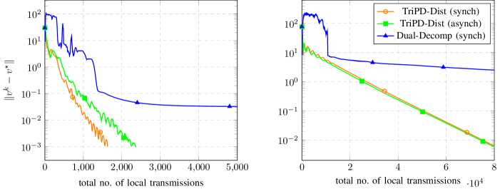
Figure 1: Comparison for the convergence of the algorithms for $m=5$ (left), and $m=50$ (right).

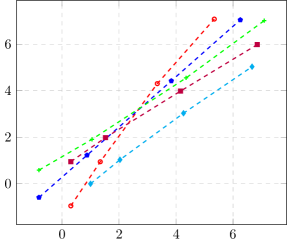
Figure 2: Five agents reorganizing from a polygon to an arrow configuration .

$$\begin{array}[m]{>{\displaystyle}r >{\displaystyle}l}\operatorname*{minimize\ }_{\mathchoice{\text{\boldmath{$\displaystyle x$}}}{\text{\boldmath{$\textstyle x$}}}{\text{\boldmath{$\scriptstyle x$}}}{\text{\boldmath{$\scriptscriptstyle x$}}}_{i},\mathchoice{\text{\boldmath{$\displaystyle u$}}}{\text{\boldmath{$\textstyle u$}}}{\text{\boldmath{$\scriptstyle u$}}}{\text{\boldmath{$\scriptscriptstyle u$}}}_{i}}{}&\sum_{i=1}^{m}\tfrac{1}{2}\|\mathcal{Q}_{i}\mathchoice{\text{\boldmath{$\displaystyle x$}}}{\text{\boldmath{$\textstyle x$}}}{\text{\boldmath{$\scriptstyle x$}}}{\text{\boldmath{$\scriptscriptstyle x$}}}_{i}-q_{i}\|^{2}+\tfrac{1}{2}\|\mathcal{R}_{i}\mathchoice{\text{\boldmath{$\displaystyle u$}}}{\text{\boldmath{$\textstyle u$}}}{\text{\boldmath{$\scriptstyle u$}}}{\text{\boldmath{$\scriptscriptstyle u$}}}_{i}-t_{i}\|^{2}\\ \hfil&\mathllap{{}+{}}\sum_{i=1}^{m}\sum_{j\in\mathcal{N}_{i}}\tfrac{\lambda_{i}}{2}\|\mathcal{C}(\mathchoice{\text{\boldmath{$\displaystyle x$}}}{\text{\boldmath{$\textstyle x$}}}{\text{\boldmath{$\scriptstyle x$}}}{\text{\boldmath{$\scriptscriptstyle x$}}}_{i}-\mathchoice{\text{\boldmath{$\displaystyle x$}}}{\text{\boldmath{$\textstyle x$}}}{\text{\boldmath{$\scriptstyle x$}}}{\text{\boldmath{$\scriptscriptstyle x$}}}_{j})-d_{ij}\|^{2}\\[14.0pt] \operatorname*{subject\ to\ }{}&\mathcal{A}_{i}\mathchoice{\text{\boldmath{$\displaystyle x$}}}{\text{\boldmath{$\textstyle x$}}}{\text{\boldmath{$\scriptstyle x$}}}{\text{\boldmath{$\scriptscriptstyle x$}}}_{i}+\mathcal{B}_{i}\mathchoice{\text{\boldmath{$\displaystyle u$}}}{\text{\boldmath{$\textstyle u$}}}{\text{\boldmath{$\scriptstyle u$}}}{\text{\boldmath{$\scriptscriptstyle u$}}}_{i}=b_{i},\ \mathchoice{\text{\boldmath{$\displaystyle x$}}}{\text{\boldmath{$\textstyle x$}}}{\text{\boldmath{$\scriptstyle x$}}}{\text{\boldmath{$\scriptscriptstyle x$}}}_{i}\in\mathcal{X}_{i},\ \mathchoice{\text{\boldmath{$\displaystyle u$}}}{\text{\boldmath{$\textstyle u$}}}{\text{\boldmath{$\scriptstyle u$}}}{\text{\boldmath{$\scriptscriptstyle u$}}}_{i}\in\mathcal{U}_{i}\\ \hfil&i=1,\ldots,m\end{array}$$ (33)

The relative desired distance of agent $i$ from its neighbor $j$ is given by $d_{ij}$, $\mathcal{C}$ is an appropriate linear mapping that selects the position variables, and $\lambda_{i}$ is an scalar weight to penalize deviation.

For each system that communicates with $i$, i.e., $j\in\mathcal{N}_{i}$, we introduce a local variable $\mathchoice{\text{\boldmath{$\displaystyle x$}}}{\text{\boldmath{$\textstyle x$}}}{\text{\boldmath{$\scriptstyle x$}}}{\text{\boldmath{$\scriptscriptstyle x$}}}_{ij}$, that can be seen as the estimate of $\mathchoice{\text{\boldmath{$\displaystyle x$}}}{\text{\boldmath{$\textstyle x$}}}{\text{\boldmath{$\scriptstyle x$}}}{\text{\boldmath{$\scriptscriptstyle x$}}}_{j}$ kept locally by agent $i$. In order to be consistent hereafter the self variables $\mathchoice{\text{\boldmath{$\displaystyle x$}}}{\text{\boldmath{$\textstyle x$}}}{\text{\boldmath{$\scriptstyle x$}}}{\text{\boldmath{$\scriptscriptstyle x$}}}_{i},\mathchoice{\text{\boldmath{$\displaystyle u$}}}{\text{\boldmath{$\textstyle u$}}}{\text{\boldmath{$\scriptstyle u$}}}{\text{\boldmath{$\scriptscriptstyle u$}}}_{i}$ are denoted by $\mathchoice{\text{\boldmath{$\displaystyle x$}}}{\text{\boldmath{$\textstyle x$}}}{\text{\boldmath{$\scriptstyle x$}}}{\text{\boldmath{$\scriptscriptstyle x$}}}_{ii},\mathchoice{\text{\boldmath{$\displaystyle u$}}}{\text{\boldmath{$\textstyle u$}}}{\text{\boldmath{$\scriptstyle u$}}}{\text{\boldmath{$\scriptscriptstyle u$}}}_{ii}$.

For each agent $i=1,\ldots,m$ define the stacked vector

$${z}_{\mathcal{N}_{i}}={\mathopen{}\left((\mathchoice{\text{\boldmath{$\displaystyle x$}}}{\text{\boldmath{$\textstyle x$}}}{\text{\boldmath{$\scriptstyle x$}}}{\text{\boldmath{$\scriptscriptstyle x$}}}_{ij})_{j\in\mathcal{N}_{i}\cup\{i\}},\mathchoice{\text{\boldmath{$\displaystyle u$}}}{\text{\boldmath{$\textstyle u$}}}{\text{\boldmath{$\scriptstyle u$}}}{\text{\boldmath{$\scriptscriptstyle u$}}}_{ii}\right)\mathclose{}}\in{{\rm I\mathchoice{}{}{}{}R}}^{n_{i}},$$

where $n_{i}=4N(|\mathcal{N}_{i}|+1)+2N$.

Let $E_{i}$ be a linear mapping such that $E_{i}z_{\mathcal{N}_{i}}=\mathcal{A}_{i}\mathchoice{\text{\boldmath{$\displaystyle x$}}}{\text{\boldmath{$\textstyle x$}}}{\text{\boldmath{$\scriptstyle x$}}}{\text{\boldmath{$\scriptscriptstyle x$}}}_{ii}+\mathcal{B}_{i}\mathchoice{\text{\boldmath{$\displaystyle u$}}}{\text{\boldmath{$\textstyle u$}}}{\text{\boldmath{$\scriptstyle u$}}}{\text{\boldmath{$\scriptscriptstyle u$}}}_{ii}$. Hence, the set of points satisfying the dynamics are given by $\mathcal{D}_{i}=\{z\in{{\rm I\mathchoice{}{}{}{}R}}^{n_{i}}|E_{i}z={b}_{i}\}$. Consider the linear mapping $L_{i}$ such that $L_{i}z_{\mathcal{N}_{i}}=(\mathchoice{\text{\boldmath{$\displaystyle x$}}}{\text{\boldmath{$\textstyle x$}}}{\text{\boldmath{$\scriptstyle x$}}}{\text{\boldmath{$\scriptscriptstyle x$}}}_{ii},\mathchoice{\text{\boldmath{$\displaystyle u$}}}{\text{\boldmath{$\textstyle u$}}}{\text{\boldmath{$\scriptstyle u$}}}{\text{\boldmath{$\scriptscriptstyle u$}}}_{ii})$ and denote $\mathcal{Z}_{i}\coloneqq\mathcal{X}_{i}\times\mathcal{U}_{i}$. Moreover, let ${h}_{i}\coloneqq\delta_{\mathcal{Z}_{i}}$, ${g}_{i}\coloneqq\delta_{\mathcal{D}_{i}}$ and

$${f}_{i}(z_{\mathcal{N}_{i}})\coloneqq \tfrac{1}{2}\|\mathcal{Q}_{i}\mathchoice{\text{\boldmath{$\displaystyle x$}}}{\text{\boldmath{$\textstyle x$}}}{\text{\boldmath{$\scriptstyle x$}}}{\text{\boldmath{$\scriptscriptstyle x$}}}_{ii}-q_{i}\|^{2}+\tfrac{1}{2}\|\mathcal{R}_{i}\mathchoice{\text{\boldmath{$\displaystyle u$}}}{\text{\boldmath{$\textstyle u$}}}{\text{\boldmath{$\scriptstyle u$}}}{\text{\boldmath{$\scriptscriptstyle u$}}}_{ii}-t_{i}\|^{2}$$

$$+\tfrac{\lambda_{i}}{2}\textstyle\sum_{j\in\mathcal{N}_{i}}\|\mathcal{C}(\mathchoice{\text{\boldmath{$\displaystyle x$}}}{\text{\boldmath{$\textstyle x$}}}{\text{\boldmath{$\scriptstyle x$}}}{\text{\boldmath{$\scriptscriptstyle x$}}}_{ii}-\mathchoice{\text{\boldmath{$\displaystyle x$}}}{\text{\boldmath{$\textstyle x$}}}{\text{\boldmath{$\scriptstyle x$}}}{\text{\boldmath{$\scriptscriptstyle x$}}}_{ij})-d_{ij}\|^{2}.$$

With these definitions problem (33) is cast in the form of problem (30) (minimizing over $z_{\mathcal{N}_{i}}$, $i=1,\ldots,m$) where the linear mapping $A_{ij}$, for $j\in\mathcal{N}_{i}$, is such that $A_{ij}z_{\mathcal{N}_{i}}=(\mathchoice{\text{\boldmath{$\displaystyle x$}}}{\text{\boldmath{$\textstyle x$}}}{\text{\boldmath{$\scriptstyle x$}}}{\text{\boldmath{$\scriptscriptstyle x$}}}_{ii},-\mathchoice{\text{\boldmath{$\displaystyle x$}}}{\text{\boldmath{$\textstyle x$}}}{\text{\boldmath{$\scriptstyle x$}}}{\text{\boldmath{$\scriptscriptstyle x$}}}_{ij})$ if $i<j$ and $A_{ij}z_{\mathcal{N}_{i}}=(-\mathchoice{\text{\boldmath{$\displaystyle x$}}}{\text{\boldmath{$\textstyle x$}}}{\text{\boldmath{$\scriptstyle x$}}}{\text{\boldmath{$\scriptscriptstyle x$}}}_{ij},\mathchoice{\text{\boldmath{$\displaystyle x$}}}{\text{\boldmath{$\textstyle x$}}}{\text{\boldmath{$\scriptstyle x$}}}{\text{\boldmath{$\scriptscriptstyle x$}}}_{ii})$ otherwise. Therefore, we can readily apply TriPD-Dist (Alg. 3) to solve the problem in a fully distributed fashion yielding both synchronous and randomized asynchronous implementations.

In our simulations we used horizon length $N=3$. For the input and state constraints of all agents we used box constraints: the positions $p_{x_{i}}$ and $p_{y_{i}}$ are assumed to be between $0$ and $20$ (m). The velocities $v_{x_{i}}$ and $v_{y_{i}}$ and inputs $v_{x_{i}}^{u}$ and $v_{y_{i}}^{u}$ are assumed to be between between $0$ and $15$ (m/s) (for all agents). The local state cost matrices are set $\mathcal{Q}_{i}=0.1I$ for all $i$. The local input cost matrices are set $\mathcal{R}_{i}=I$ for half of the agents and $\mathcal{R}_{i}=2I$ for the rest. Moreover, the vectors $q_{i}$, $t_{i}$ are set equal to zero, and the penalty parameter $\lambda_{i}=10$ is used for all the agents.

The stepsizes of TriPD-Dist (Alg. 3) were selected as follows: i) (edge stepsizes) $\kappa_{(i,j)}=1$ for all $(i,j)\in\mathcal{E}$, ii) (node stepsizes) $\sigma_{i}=\beta_{i}/4$ and $\tau_{i}=0.99/(\tfrac{\beta_{i}}{2}+\sigma_{i}+\sum_{j\in\mathcal{N}_{i}}\kappa_{(i,j)})$ for all $i$, where we used

$$\beta_{i}=\max\{\|\mathcal{Q}_{i}^{\top}\mathcal{Q}_{i}\|+\lambda_{i}(|\mathcal{N}_{i}|+1),\|\mathcal{R}_{i}^{\top}\mathcal{R}_{i}\|\},$$

which is an upper bound for the Lipschitz constant of $\nabla f_{i}$. It is plain to see that the above choice of stepsizes for the agents satisfy Item 3). Note that the stepsize selection only requires local parameters $\mathcal{R}_{i}$, $\mathcal{Q}_{i}$, $\lambda_{i}$ and the number of neighbors $|\mathcal{N}_{i}|$, i.e., the algorithm can be implemented without any global coordination.

In our simulations, we considered $m$ robots initially in a polygon configuration and enforced an arrow formation by appropriate selection of $d_{ij}$ in (33). This scenario is depicted for $m=5$ in Figure 2. The neighborhood relation in this case is taken to be the same arrow configuration, i.e., all agents have two neighbors apart from two agents with only one neighbor.

For comparison we considered the dual decomposition approach of [15] (based on the subgradient method). Notice that dual decomposition with gradient or accelerated gradient methods can not be applied to this problem since ${f}_{i}$’s are convex but not strongly convex. Recently, TriPD-Dist (Alg. 3) was compared against the dual accelerated proximal gradient method, in the context of distributed model predictive control (with strongly convex quadratic cost) [36].

In the simulations for Figure 1, we used the stepsize $10/k$ (as tuned for achieving better performance) for the dual decomposition method where $k$ is the number of iterations. Notice that the dual decomposition approach for this problem can not achieve a full splitting of the operators involved: at every iteration agents need to solve an inner minimization (we used MATLAB’s quadprog to perform this step), the result of which must be communicated to the neighbors for their computation, and is followed by another communication round. This extra need for synchronization would further slow down the algorithm in practical implementations [37].

Figure 1 demonstrates the superior performance of both the synchronous and asynchronous versions of TriPD-Dist (Alg. 3) compared to the dual decomposition approach. The $y$-axis is the distance of $v^{k}\coloneqq(\mathchoice{\text{\boldmath{$\displaystyle x$}}}{\text{\boldmath{$\textstyle x$}}}{\text{\boldmath{$\scriptstyle x$}}}{\text{\boldmath{$\scriptscriptstyle x$}}}_{11}^{k},\mathchoice{\text{\boldmath{$\displaystyle u$}}}{\text{\boldmath{$\textstyle u$}}}{\text{\boldmath{$\scriptstyle u$}}}{\text{\boldmath{$\scriptscriptstyle u$}}}_{11}^{k},\ldots,\mathchoice{\text{\boldmath{$\displaystyle x$}}}{\text{\boldmath{$\textstyle x$}}}{\text{\boldmath{$\scriptstyle x$}}}{\text{\boldmath{$\scriptscriptstyle x$}}}_{mm}^{k},\mathchoice{\text{\boldmath{$\displaystyle u$}}}{\text{\boldmath{$\textstyle u$}}}{\text{\boldmath{$\scriptstyle u$}}}{\text{\boldmath{$\scriptscriptstyle u$}}}_{mm}^{k})$ from the solution ($v^{\star}$ was computed by solving (33) in a centralized fashion). The $x$-axis denotes the total number of local transmissions between agents. In the asynchronous implementation we used independent activation probabilities $p_{i}=0.5$ for all agents. It is observed that the total number of local iterations is similar to that of the synchronous implementation. Finally, as evident in Figure 1 both versions of TriPD-Dist (Alg. 3) achieve linear convergence rate as predicted by Theorems V.1 and V.2 (the functions $f_{i},g_{i}$ and $h_{i}$ are PLQ).

VII Conclusions

The primal-dual algorithm introduced in this paper enjoys several structural properties that distinguish it from other related methods in the literature. A key property, that has been instrumental in developing a block-coordinate version of the algorithm, is the fact that the generated sequence is $S$-Fejér monotone, where $S$ is a block diagonal positive definite matrix. It is shown that the algorithm attains linear convergence under a metric subregularity assumption that holds for a wide range of cost functions that are not necessarily strongly convex. The block-coordinate version of the developed algorithm is exploited to devise a novel fully distributed asynchronous method for multi-agent optimization over graphs. Our future work includes designing a block-coordinate version of the SuperMann scheme of [38] that applies to quasi-nonexpansive operators. In light of the fact that this method enjoys superlinear convergence rates, such extension is especially attractive for multi-agent optimization yielding schemes with faster convergence and fewer communication rounds. Other research directions enlist investigating extensions to account for directed and time-varying topologies, communication delays, and designing efficient strategies for selecting activation probabilities and stepsizes.

Appendix A

Proof of Lemma II.4.

Consider the operator $T$ as in (12). By monotonicity of $A$ at $z^{\star}$ and $\bar{z}$ along with (13) we have

$$0\leq\langle-Mz^{\star}-Cz^{\star}+Mz+Cz-Hz+H\bar{z},z^{\star}-\bar{z}\rangle.$$ (34)

For $\beta_{f}>0$, item 2) is equivalent to $\nabla f$ being cocoercive [17, Thm. 18.16], i.e., for all $x,y\in{{\rm I\mathchoice{}{}{}{}R}}^{n}$:

$$\tfrac{1}{\beta_{f}}\|\nabla f(x)-\nabla f(y)\|_{Q^{-1}}^{2}\leq\langle\nabla f(x)-\nabla f(y),x-y\rangle.$$ (35)

On the other hand, for $\beta_{f}>0$ we have

$$\langle Cz-Cz^{\star} ,z^{\star}-\bar{z}\rangle=\langle\nabla f(x)-\nabla f({x}^{\star}),x^{\star}-\bar{x}\rangle$$

$$={} \langle\nabla f(x)-\nabla f({x}^{\star}),x-\bar{x}\rangle$$

$$+\langle\nabla f(x)-\nabla f({x}^{\star}),x^{\star}-x\rangle$$

$$\leq{} \tfrac{1}{\beta_{f}}\|\nabla f(x)-\nabla f(x^{\star})\|_{Q^{-1}}^{2}+\tfrac{\beta_{f}}{4}\|x-\bar{x}\|_{Q}^{2}$$

$$+\langle\nabla f(x)-\nabla f({x}^{\star}),x^{\star}-x\rangle$$

$$\leq{} \langle\nabla f(x)-\nabla f({x}^{\star}),x-x^{\star}\rangle+\tfrac{\beta_{f}}{4}\|x-\bar{x}\|_{Q}^{2}$$

$$+\langle\nabla f(x)-\nabla f({x}^{\star}),x^{\star}-x\rangle,$$

$$={} \tfrac{\beta_{f}}{4}\|x-\bar{x}\|_{Q}^{2},$$ (36)

where we have used (2) (with $V=\tfrac{2}{\beta_{f}}Q^{-1}$) in the first inequality, and (35) in the second inequality, respectively. Notice that if $\beta_{f}=0$ then inequality (36) holds trivially with equality.

Using (36) in (34), along with skew-symmetry of $K$ and $M$, we have

$$0\leq \langle-Mz^{\star}-Cz^{\star}+Mz+Cz-Hz+H\bar{z},z^{\star}-\bar{z}\rangle$$

$$\leq \langle(M-K)({z}-z^{\star})+P(\bar{z}-{z}),z^{\star}-\bar{z}\rangle+\tfrac{\beta_{f}}{4}\|{x}-\bar{{x}}\|_{Q}^{2}$$

$$= \langle(M-K)({z}-z^{\star})+P(\bar{z}-{z}),z^{\star}-{z}\rangle+\tfrac{\beta_{f}}{4}\|{x}-\bar{{x}}\|_{Q}^{2}$$

$$+\langle(M-K)({z}-z^{\star})+P(\bar{z}-{z}),{z}-\bar{z}\rangle$$

$$= \langle P(\bar{z}-{z}),z^{\star}-{z}\rangle+\tfrac{\beta_{f}}{4}\|{x}-\bar{{x}}\|_{Q}^{2}-\|\bar{z}-{z}\|_{P}^{2}$$

$$+\langle(M-K)({z}-z^{\star}),{z}-\bar{z}\rangle$$

$$= \langle{z}-z^{\star},(H+M^{\top})({z}-\bar{z})\rangle$$

$$+\tfrac{\beta_{f}}{4}\|{x}-\bar{x}\|_{Q}^{2}-\|\bar{z}-{z}\|_{P}^{2}.$$ (37)

By definition, $S^{-1}(H+M^{\top})(\bar{z}-z)=Tz-z$. Thus

$$\langle{z}-z^{\star},(H+M^{\top})({z}-\bar{z})\rangle =\langle{z}-z^{\star},{z}-Tz\rangle_{S}.$$ (38)

On the other hand, we have $\bar{z}-z=(H+M^{\top})^{-1}S(Tz-z)$. Using (10), (14) and (7c) we conclude

$$\|\bar{z}-z\|_{P}^{2}-\tfrac{\beta_{f}}{4}\|\bar{{x}}-{x}\|_{Q}^{2}=\|Tz-z\|_{\tilde{P}}^{2},$$ (39)

where $\tilde{P}$ is defined in (16). Combining (37), (38) and (39) completes the proof. ∎

Proof of Theorem II.5.

We establish convergence by showing that the sequence $(z^{k})_{k\in{{\rm I\mathchoice{}{}{}{}N}}}$ is Fejér monotone with respect to $\mathcal{S}=\operatorname*{fix}T$. We have

$$\|z^{k+1}-z^{\star}\|_{S}^{2}= \|Tz^{k}-z^{k}+z^{k}-z^{\star}\|_{S}^{2}$$

$$={} \|z^{k}-z^{\star}\|_{S}^{2}+\|Tz^{k}-z^{k}\|_{S}^{2}$$

$$+2\langle z^{k}-z^{\star},Tz^{k}-z^{k}\rangle_{S}$$

$$\leq{} \|z^{k}-z^{\star}\|_{S}^{2}-\|Tz^{k}-z^{k}\|_{2{\tilde{P}}-S}^{2},$$ (40)

where the inequality follows from Lemma II.4. Note that $2\tilde{P}-S$ is symmetric positive-definite if and only if Assumption 2 holds. Therefore, by (40) the sequence $(z^{k})_{k\in{{\rm I\mathchoice{}{}{}{}N}}}$ is Fejér monotone in the space equipped with inner product $\langle\cdot,\cdot\rangle_{S}$; in particular, $(z^{k})_{k\in{{\rm I\mathchoice{}{}{}{}N}}}$ is bounded. Furthermore, it follows from (40) and the fact that $2\tilde{P}-S$ is positive-definite that

$$\|Tz^{k}-z^{k}\|\rightarrow 0.$$ (41)

The operator $T$ is continuous (since it involves proximal and linear mappings that are continuous, and since $\nabla f$ is assumed continuous). Let $z^{c}$ be a cluster point of $(z^{k})_{k\in{{\rm I\mathchoice{}{}{}{}N}}}$. It follows from the continuity of $T$ and (41) that $Tz^{c}-z^{c}=0$, i.e., $z^{c}\in\operatorname*{fix}T$. The result follows from Fejér monotonicity of $(z^{k})_{k\in{{\rm I\mathchoice{}{}{}{}N}}}$ with respect to $\mathcal{S}=\operatorname*{fix}T$ and [17, Thm. 5.5]. ∎

Proof of Theorem III.1.

Let us define the operator $E^{k}\coloneqq\sum_{i=1}^{m}\epsilon^{k}_{i}U_{i}$ that maps the elements of $({{\rm I\mathchoice{}{}{}{}R}}^{n+r},\mathcal{F}_{k-1})$ to $({{\rm I\mathchoice{}{}{}{}R}}^{n+r},\mathcal{F}_{k})$. The iterations of TriPD-BC (Alg. 2) can be written as $z^{k+1}=z^{k}+E^{k+1}(Tz^{k}-z^{k})$. We have

$$\mathbb{E}_{k}\circ E^{k+1}=\sum_{\varepsilon\in\Psi}\mathbb{P}(\epsilon^{k+1}=\varepsilon)\sum_{j=1}^{m}\varepsilon_{j}U_{j}$$

$$=\sum_{j=1}^{m}\sum_{\varepsilon\in\Psi}\mathbb{P}(\epsilon^{k+1}=\varepsilon)\varepsilon_{j}U_{j}$$

$$=\sum_{j=1}^{m}\sum_{\varepsilon\in\Psi,\varepsilon_{j}=1}\mathbb{P}(\epsilon^{k+1}=\varepsilon)U_{j}=\sum_{j=1}^{m}p_{j}U_{j}=\Pi,$$ (42)

where we used Items 2) and 1). Therefore, we have

$$\mathbb{E}_{k} {\mathopen{}\left[\|z^{k+1}-z^{\star}\|_{\Pi^{-1}S}^{2}\right]\mathclose{}}$$

$$={} \mathbb{E}_{k}{\mathopen{}\left[\|z^{k}+E^{k+1}(Tz^{k}-{{z}^{k}})-z^{\star}\|_{\Pi^{-1}S}^{2}\right]\mathclose{}}$$

$$={} \|z^{k}-z^{\star}\|_{\Pi^{-1}S}^{2}+2\langle z^{k}-z^{\star},\mathbb{E}_{k}{\mathopen{}\left[E^{k+1}(Tz^{k}-{{z}^{k}})\right]\mathclose{}}\rangle_{\Pi^{-1}S}$$

$$+\mathbb{E}_{k}{\mathopen{}\left[\langle E^{k+1}(Tz^{k}-z^{k}),E^{k+1}(Tz^{k}-z^{k})\rangle_{\Pi^{-1}S}\right]\mathclose{}}$$

$$={} \|z^{k}-z^{\star}\|_{\Pi^{-1}S}^{2}+\|Tz^{k}-z^{k}\|_{S}^{2}$$

$$+2\langle z^{k}-z^{\star},Tz^{k}-z^{k}\rangle_{S}$$

where we used (42) and the fact $E^{k}$ is self-adjoint and idempotent (since $U_{i}$ are $0$-$1$ matrices) in the last equality. Inequality (28) follows by using (17). The convergence of the sequence follows from (28) using the Robbins-Siegmund lemma [26] and arguing as in [7, Thm. 3] and [8, Prop. 2.3]. ∎

Proof of Lemma IV.2.

From the equivalent characterization of strong subregularity in (29) we have that there exists a neighborhood $\mathcal{U}_{{x}^{\star}}$ of ${x}^{\star}$ such that for all $x\in\mathcal{U}_{x^{\star}}$

$$(f+g)(x)\geq (f+g)(x^{\star})+\langle-L^{\top}u^{\star},x-x^{\star}\rangle$$

$$+c_{1}\|x-x^{\star}\|^{2},$$ (43)

and a neighborhood $\mathcal{U}_{{u}^{\star}}$ of ${u}^{\star}$ such that for all $u\in\mathcal{U}_{u^{\star}}$

$$h^{*}(u)\geq h^{*}(u^{\star})+\langle Lx^{\star},u-u^{\star}\rangle+c_{2}\|u-u^{\star}\|^{2}.$$

Fix $z=(u,x)$ with $u\in\mathcal{U}_{u^{\star}}$ and $x\in\mathcal{U}_{x^{\star}}$. Consider $v=(v_{1},v_{2})\in Fz\coloneqq Az+Mz+Cz$. By definition (cf. (8)) we have

$${\mathopen{}\left\{\begin{array}[]{@{}l@{}l@{}}v_{1}\in\partial h^{*}(u)-Lx,&\\ v_{2}\in\partial g(x)+\nabla f(x)+L^{\top}u.&\end{array}\right.\mathclose{}}$$

Using this together with the definition of subdifferential yields:

$$\langle v_{1}+Lx,u-{u}^{\star}\rangle \geq h^{*}(u)-h^{*}({u}^{\star}),$$ (45)

$$\langle v_{2}-L^{\top}u,x-x^{\star}\rangle \geq(f+g)(x)-(f+g)(x^{\star}).$$ (46)

Combining (45), (46) with (43), (A) and noting that

$$\langle L^{\top}(u^{\star}-u),x-x^{\star}\rangle+\langle L(x-x^{\star}),u-u^{\star}\rangle=0,$$

yields:

$$\langle v,z-{z}^{\star}\rangle =\langle v_{1},u-{u}^{\star}\rangle+\langle v_{2},x-{x}^{\star}\rangle$$

$$\geq c_{2}\|u-{u}^{\star}\|^{2}+c_{1}\|x-{x}^{\star}\|^{2}\geq c\|z-z^{\star}\|^{2},$$

where $c=\min\{c_{1},c_{2}\}$. Therefore, by the Cauchy-Schwarz inequality $\|v\|\geq c\|z-z^{\star}\|$. Since $\|z-z^{\star}\|\geq d(z,F^{-1}0)$, and $v\in Fz$ was selected arbitrarily, we have

$$d(z,F^{-1}0)\leq\tfrac{1}{c}d(0,Fz)\quad\forall z\in{\mathcal{U}_{u^{\star}}}\times{\mathcal{U}_{x^{\star}}}.$$ (47)

Thus $F$ is metrically subregular at $z^{\star}$ for $0$.

To establish uniqueness of the primal-dual solution consider:

$$\mathcal{L}(u,x)\coloneqq(f+g)(x)+\langle Lx,u\rangle-h^{*}(u).$$

Adding (43) and (A) yields

$$\mathcal{L}(u^{\star},x)-\mathcal{L}(u,x^{\star})\geq c\|z-z^{\star}\|^{2}\quad\forall z\in{\mathcal{U}_{u^{\star}}}\times{\mathcal{U}_{x^{\star}}}$$ (48)

Let $\bar{z}^{\star}=(\bar{u}^{\star},\bar{x}^{\star})\in\mathcal{S}$ such that $\bar{z}^{\star}\in\mathcal{U}_{u^{\star}}\times\mathcal{U}_{x^{\star}}$. Since $\bar{z}^{\star}$ is also a primal-dual solution we have $\mathcal{L}(\bar{u}^{\star},x^{\star})-\mathcal{L}(u^{\star},\bar{x}^{\star})\geq 0$. Therefore, using (48) at $\bar{z}^{\star}$ yields $\bar{z}^{\star}=z^{\star}$. Since $\mathcal{S}$ is convex, we conclude that it is a singleton, i.e., $\mathcal{S}=\{z^{\star}\}$. Consequently it follows from (47) that $F$ is strongly subregular at $z^{\star}$ for $0$.

The second part is a direct consequence of the first part and the fact that if Assumption 4 holds globally then also the quadratic growth conditions (43) and (A) hold globally, i.e., $\mathcal{U}_{x^{\star}}={{\rm I\mathchoice{}{}{}{}R}}^{n}$, $\mathcal{U}_{u^{\star}}\in{{\rm I\mathchoice{}{}{}{}R}}^{r}$. This can be shown by adapting the proof of [29, Thm. 3.3]. ∎

Proof of Lemma IV.4.

Since $f$, $g$ and $h$ are proper closed convex PLQ, the subdifferentials $\partial g$, $\nabla f$ and $\partial h^{*}$ are piecewise polyhedral mappings [16, Prop. 12.30(b), Thm. 11.14(b)]. The graph of $M$ is polyhedral, since $M$ is linear. Therefore, the sum $F=A+M+C$ is also piecewise polyhedral. Since the inverse of a piecewise polyhedral mapping is piecewise polyhedral, the result follows from [27, 3H.1 and 3H.3]. ∎

Proof of Theorem IV.6.

For notational convenience let $\bar{S}=\Pi^{-1}S$ and note that $\mathcal{S}=\operatorname*{zer}F$ (cf. (15)). By definition we have $\|{z}^{k}-\mathcal{P}^{\bar{S}}_{\mathcal{S}}({z}^{k})\|_{\bar{S}}=d_{\bar{S}}({z}^{k},\mathcal{S})$ (where the minimum is attained since $\mathcal{S}$ is a closed convex set). Consequently, it follows from (28) that

$${\operatorname*{\mathbb{E}}}_{k}{\mathopen{}\left[d^{2}_{\bar{S}}({z}^{k+1},\mathcal{S})\right]\mathclose{}} \leq{\operatorname*{\mathbb{E}}}_{k}{\mathopen{}\left[\|z^{k+1}-\mathcal{P}^{\bar{S}}_{\mathcal{S}}(z^{k})\|^{2}_{\bar{S}}\right]\mathclose{}}$$

$$\leq\|z^{k}-\mathcal{P}^{\bar{S}}_{\mathcal{S}}(z^{k})\|_{\bar{S}}^{2}-\|T{z}^{k}-{z}^{k}\|_{2\tilde{P}-S}^{2}$$

$$=d_{\bar{S}}^{2}(z^{k},\mathcal{S})-\|T{z}^{k}-{z}^{k}\|_{2\tilde{P}-S}^{2}.$$ (49)

By definition (12), we have

$$\|\bar{z}^{k}-z^{k}\|^{2}=\|(H+M^{\top})^{-1}S(Tz^{k}-z^{k})\|^{2}$$

$$\leq\|(H+M^{\top})^{-1}S\|^{2}\|{(2\tilde{P}-S)}^{-1}\|\|Tz^{k}-z^{k}\|^{2}_{2\tilde{P}-S},$$ (50)

where $\bar{z}^{k}$ is defined by (13) applied at $z=z^{k}$. Consider the projection of $\bar{z}^{k}$ onto $\mathcal{S}$, $\mathcal{P}_{\mathcal{S}}(\bar{z}^{k})$. By definition $\|\bar{z}^{k}-\mathcal{P}_{\mathcal{S}}(\bar{z}^{k})\|=d(\bar{z}^{k},\mathcal{S})$, and we have

$$d_{\bar{S}}^{2}(z^{k},\mathcal{S}) \leq\|z^{k}-\mathcal{P}_{\mathcal{S}}(\bar{z}^{k})\|_{\bar{S}}^{2}\leq\|{\bar{S}}\|\|z^{k}-\mathcal{P}_{\mathcal{S}}(\bar{z}^{k})\|^{2}$$

$$\leq\|{\bar{S}}\|{\mathopen{}\left(\|\bar{z}^{k}-\mathcal{P}_{\mathcal{S}}(\bar{z}^{k})\|+\|\bar{z}^{k}-z^{k}\|\right)\mathclose{}}^{2}$$

$$=\|{\bar{S}}\|{\mathopen{}\left(d(\bar{z}^{k},\mathcal{S})+\|\bar{z}^{k}-z^{k}\|\right)\mathclose{}}^{2}.$$ (51)

In what follows we bound $d(\bar{z}^{k},\mathcal{S})$ by $\|\bar{z}^{k}-z^{k}\|$. Define

$$v^{k}\coloneqq-(H-M)(\bar{z}^{k}-z^{k})+C\bar{z}^{k}-Cz^{k}.$$ (52)

It follows from (13) that $(H-M-C)z^{k}\in(H+D)\bar{z}^{k}$, which in turn implies

$$v^{k}\in F\bar{z}^{k}=(A+M+C)\bar{z}^{k}.$$

Consequently, using (global) metric subregularity of $F$ yields

$$d(\bar{z}^{k},\mathcal{S})\leq\eta\|v^{k}\|.$$ (53)

By the triangle inequality and Lipschitz continuity of $C$,

$$\|v^{k}\|=\|(H-M)(\bar{z}^{k}-z^{k})-C\bar{z}^{k}+C{z^{k}}\|$$

$$\leq\|(H-M)(\bar{z}^{k}-z^{k})\|+\|C\bar{z}^{k}-Cz^{k}\|\leq\xi\|\bar{z}^{k}-z^{k}\|,$$ (54)

where $\xi=\|H\!-\!M\|+\beta_{f}\|Q\|$. By (53) and (54) we have

$$d(\bar{z}^{k},\mathcal{S})\leq\xi\eta\|\bar{z}^{k}-z^{k}\|.$$

Combine this with (50) and (51) to derive

$$d_{\bar{S}}^{2}(z^{k},\mathcal{S})\leq\phi\|Tz^{k}-z^{k}\|^{2}_{2\tilde{P}-S},$$ (55)

where $\phi=(\xi\eta+1)^{2}\|(H+M^{\top})^{-1}S\|^{2}\|{(2\tilde{P}-S)}^{-1}\|\|\bar{S}\|$. Therefore, by (49) and (55) we have

$${\operatorname*{\mathbb{E}}}_{k}{\mathopen{}\left[d^{2}_{\bar{S}}({z}^{k+1},\mathcal{S})\right]\mathclose{}}\leq d_{\bar{S}}^{2}(z^{k},\mathcal{S})-\tfrac{1}{\phi}d_{\bar{S}}^{2}(z^{k},\mathcal{S}).$$

Taking expectation in both sides concludes the proof. For the case of PLQ functions, let $\mathcal{U}_{z_{\star}}$ denote an open subregularity neighborhood around $z_{\star}\in\mathcal{S}$, and set $\mathcal{U}_{\star}\coloneqq\cup_{z^{\star}\in\mathcal{S}}\mathcal{U}_{z_{\star}}$. By Lemma IV.4 there exists a positive $\eta$ such that $d(z,F^{-1}0)\leq\eta d(0,Fz)$ for $z\in\mathcal{U}_{\star}$. Moreover, since $(z^{k})_{k\in{{\rm I\mathchoice{}{}{}{}N}}}\subseteq\mathcal{C}$ up to possibly enlarging $\mathcal{C}$ we have $(\bar{z}^{k})_{k\in{{\rm I\mathchoice{}{}{}{}N}}}\subseteq\mathcal{C}$. Note that since $(z^{k})_{k\in{{\rm I\mathchoice{}{}{}{}N}}}\subseteq\mathcal{C}$ and $\mathcal{C}$ is closed, $\mathcal{C}\cap\mathcal{S}\neq\emptyset$ and $\mathcal{C}\cap\mathcal{U}_{\star}\neq\emptyset$. It is sufficient to show that $d(z,F^{-1}0)\leq\eta^{\prime}d(0,Fz)$ for $z\in\mathcal{C}$. Let us define $D(z)\coloneqq d(0,Fz)$. Since $\operatorname{gra}F$ is closed, $D(z)$ is lower semicontinuous [16, Thm. 5.7, Prop. 5.11(a)]. By [16, Cor. 1.10] $D(z)$ attains a minimum over the compact set $\mathcal{C}\setminus\mathcal{U}_{\star}$: $c_{d}\coloneqq\min_{z\in\mathcal{C}\setminus\mathcal{U}_{\star}}D(z)>0$ where the strict inequality is due to the fact that the minimizer belongs to $\mathcal{C}\setminus\mathcal{U}_{\star}$. Moreover, $c_{\mathcal{C}}\coloneqq\sup_{z\in\mathcal{C}}d(z,F^{-1}0)<\infty$ due to the fact that $\mathcal{C}$ is bounded. Hence $d(z,F^{-1}0)\leq c_{\mathcal{C}}\leq\tfrac{c_{\mathcal{C}}}{c_{d}}d(0,Fz)$ for $z\in\mathcal{C}\setminus\mathcal{U}_{\star}$. Therefore, by combining the two cases we obtain $d(z,F^{-1}0)\leq\max\{\tfrac{c_{\mathcal{C}}}{c_{d}},\eta\}d(0,Fz)$ for $z\in\mathcal{C}$ as claimed. The second sufficient condition follows from Lemma IV.2. ∎

Proof of Lemma IV.7.

First we show the if statement: assume that $R={\rm Id}-T$ is metrically subregular at $z^{\star}$ for $0$. Then there exists $\eta>0$ and a neighborhood $\mathcal{U}$ of $z^{\star}$ such that

$$d(z,R^{-1}0)\leq\eta d(0,Rz)\quad\forall z\in\mathcal{U}.$$ (56)

The two sets $R^{-1}0$ and $F^{-1}0$ are equal, cf. (15). In what follows, we upper bound $d(0,Rz)$ by $d(0,Fz)$. Let $w\in Fz=A{z}+M{z}+C{z}$. By (13) we have that

$$Hz-Mz-Cz-H\bar{z}\in A\bar{z}.$$

Using this together with the monotonicity of $A$ at $z$ and $\bar{z}$, we obtain:

$$0\leq \langle z-\bar{z},{\mathopen{}\left(w-M{z}-Cz\right)\mathclose{}}-{\mathopen{}\left(Hz-Mz-Cz-H\bar{z}\right)\mathclose{}}\rangle$$

$$= \langle z-\bar{z},w-Hz+H\bar{z}\rangle=\langle z-\bar{z},w\rangle-\|\bar{z}-z\|_{P}^{2},$$

where in the last equality we have used the fact that $H=P+K$ and $K$ is skew-symmetric.

By the Cauchy–Schwarz inequality

$$\|\bar{z}-z\|_{P}^{2}\leq\langle z-\bar{z},w\rangle\leq\|\bar{z}-z\|_{P}\|w\|_{P^{-1}},$$

therefore

$$\|\bar{z}-z\|_{P}\leq\|w\|_{P^{-1}}.$$ (57)

On the other hand by (12):

$$\|Rz\|\leq\|S^{-1}(H+M^{\top})P^{-1/2}\|\|\bar{z}-z\|_{P}.$$

Combine this with (56) and (57) to obtain

$$d(z,F^{-1}0)= d(z,R^{-1}0)\leq\eta\|Rz\|$$

$$\leq \eta\|S^{-1}(H+M^{\top})P^{-1/2}\|\|P^{-1}\|^{1/2}\|w\|.$$

Since $w\in Fz$ was arbitrary, we conclude that $F$ is metrically subregular at $z^{\star}$ for $0$ (with a different subregularity modulus).

Next we prove the only if statement: assume that $F$ is metrically subregular at $z^{\star}$ for $0$, i.e., there exists $\eta>0$ and neighborhood $\mathcal{U}$ of $z^{\star}$ such that

$$d(z,F^{-1}0)\leq\eta d(0,Fz)\quad\forall z\in\mathcal{U}.$$ (58)

By (37) and the Cauchy–Schwarz inequality we infer that

$$\|\bar{z}-z\|\leq c\|z-z^{\star}\|,$$

for some positive constant $c$. Hence, there exists a neighborhood $\bar{\mathcal{U}}\subset\mathcal{U}$ of $z^{\star}$ such that if $z\in\bar{\mathcal{U}}$ then $\bar{z}\in\mathcal{U}$. Fix a point $z\in\bar{\mathcal{U}}$ so that $\bar{z}\in\mathcal{U}$. By (58) it holds that:

$$d(\bar{z},F^{-1}0)\leq\eta d(0,F\bar{z}).$$ (59)

Define $v$ as in (52) (dropping the iteration index $k$). Noting that $v\in F\bar{z}$, it follows from (59) that

$$d(\bar{z},F^{-1}0)\leq\eta\|v\|\leq\eta\xi\|\bar{z}-z\|,$$ (60)

where we used (54) in the second inequality. Invoking triangle inequality we have

$$d({z},{R}^{-1}0)= d({z},F^{-1}0)\leq d(\bar{z},F^{-1}0)+\|\bar{z}-z\|$$

$$\leq (1+\eta\xi)\|\bar{z}-z\|.$$ (61)

On the other hand by (12) it holds that

$$\|\bar{z}-z\|\leq\|(H+M^{\top})^{-1}S\|\|Rz\|.$$

Combining this with (61) yields

$$d({z},{R}^{-1}0)\leq(1+\eta\xi)\|(H+M^{\top})^{-1}S\|\|Rz\|\quad\forall z\in\bar{\mathcal{U}},$$

i.e., that $R$ is metrically subregular at $z^{\star}$ for $0$. ∎

Puya Latafat is currently working towards a joint PhD at the Department of Electrical Engineering (ESAT) of KU Leuven (Belgium) and IMT School for Advanced Studies Lucca (Italy). He received his M.Sc. in Mathematical Engineering jointly from University of L’Aquila (Italy) and University of Hamburg (Germany), and his B.Sc. in Electrical Engineering from University of Tabriz (Iran). His research interests revolve around large-scale and distributed optimization with applications to model predictive control and machine learning.

Nikolaos M. Freris is Professor with the School of Computer Science and Technology at the University of Science and Technology of China (USTC). He received a Diploma in Electrical and Computer Engineering from the National Technical University of Athens, Greece in 2005, an M.S. degree in Electrical and Computer Engineering, an M.S. degree in Mathematics, and a Ph.D. degree in Electrical and Computer Engineering all from the University of Illinois at Urbana-Champaign in 2007, 2008, and 2010, respectively. Dr. Freris’s research interests lie in the area of cyberphysical systems: distributed estimation, optimization, and control, machine learning, wireless networks, signal processing, and applications in transportation, sensor networks, robotics, and power systems. His research was recognized with the 1000-talents award, the IBM High Value Patent award, two IBM invention achievement awards, and the Gerondelis foundation award. Previously, Dr. Freris was Assistant Professor of Electrical and Computer Engineering at New York University Abu Dhabi, and Global Network Assistant Professor of Computer Science at NYU Tandon School of Engineering. Dr. Freris is a senior member of IEEE, and a member of ACM and SIAM.

Panagiotis (Panos) Patrinos is assistant professor at the Department of Electrical Engineering (ESAT) of KU Leuven, Belgium since 2015. During fall/winter 2014 he held a visiting assistant professor position at Stanford University. He received his PhD in Control and Optimization, M.S. in Applied Mathematics and M.Eng. from National Technical University of Athens, in 2010, 2005 and 2003, respectively. After his PhD he held postdoc positions at the University of Trento and IMT Lucca, Italy, where he became an assistant professor in 2012. His current research interests are in the theory and algorithms of structured convex and nonconvex optimization and predictive control with a focus on large-scale, distributed, stochastic and embedded optimization and a wide range of application areas including smart grids, water networks, automotive, aerospace, machine learning and signal processing.

References

• [1] P. L. Combettes and J.-C. Pesquet, “Proximal splitting methods in signal processing,” in Fixed-Point Algorithms for Inverse Problems in Science and Engineering.   Springer New York, 2011, pp. 185–212.
• [2] B. C. Vũ, “A splitting algorithm for dual monotone inclusions involving cocoercive operators,” Advances in Computational Mathematics, vol. 38, no. 3, pp. 667–681, 2013.
• [3] L. Condat, “A primal-dual splitting method for convex optimization involving Lipschitzian, proximable and linear composite terms,” Journal of Optimization Theory and Applications, vol. 158, no. 2, pp. 460–479, 2013.
• [4] P. L. Combettes, L. Condat, J.-C. Pesquet, and B. C. Vũ, “A forward-backward view of some primal-dual optimization methods in image recovery,” in IEEE International Conference on Image Processing (ICIP), 2014, pp. 4141–4145.
• [5] Y. Nesterov, “Efficiency of coordinate descent methods on huge-scale optimization problems,” SIAM Journal on Optimization, vol. 22, no. 2, pp. 341–362, 2012.
• [6] P. Richtárik and M. Takáč, “Iteration complexity of randomized block-coordinate descent methods for minimizing a composite function,” Mathematical Programming, vol. 144, no. 1-2, pp. 1–38, 2014.
• [7] P. Bianchi, W. Hachem, and F. Iutzeler, “A coordinate descent primal-dual algorithm and application to distributed asynchronous optimization,” IEEE Transactions on Automatic Control, vol. 61, no. 10, pp. 2947–2957, Oct 2016.
• [8] P. L. Combettes and J.-C. Pesquet, “Stochastic quasi-Fejér block-coordinate fixed point iterations with random sweeping,” SIAM Journal on Optimization, vol. 25, no. 2, pp. 1221–1248, 2015.
• [9] J.-C. Pesquet and A. Repetti, “A class of randomized primal-dual algorithms for distributed optimization,” Journal of Nonlinear and Convex Analysis, vol. 16, no. 12, pp. 2453–2490, 2015.
• [10] O. Fercoq and P. Bianchi, “A coordinate descent primal-dual algorithm with large step size and possibly non separable functions,” arXiv preprint arXiv:1508.04625, 2015.
• [11] G. Zhang and R. Heusdens, “Bi-alternating direction method of multipliers over graphs,” in IEEE International Conference on Acoustics, Speech and Signal Processing (ICASSP), 2015, pp. 3571–3575.
• [12] P. Latafat, L. Stella, and P. Patrinos, “New primal-dual proximal algorithm for distributed optimization,” in 55th IEEE Conference on Decision and Control (CDC), 2016, pp. 1959–1964.
• [13] S. Boyd, A. Ghosh, B. Prabhakar, and D. Shah, “Randomized gossip algorithms,” IEEE Transactions on Information Theory, vol. 52, no. 6, pp. 2508–2530, 2006.
• [14] A. Jadbabaie, J. Lin, and A. S. Morse, “Coordination of groups of mobile autonomous agents using nearest neighbor rules,” IEEE Transactions on Automatic Control, vol. 48, no. 6, pp. 988–1001, 2003.
• [15] R. L. Raffard, C. J. Tomlin, and S. P. Boyd, “Distributed optimization for cooperative agents: application to formation flight,” in 43rd IEEE Conference on Decision and Control (CDC), vol. 3, 2004, pp. 2453–2459.
• [16] R. T. Rockafellar and R. J.-B. Wets, Variational analysis.   Springer Science & Business Media, 2009, vol. 317.
• [17] H. H. Bauschke and P. L. Combettes, Convex analysis and monotone operator theory in Hilbert spaces.   Springer Science & Business Media, 2011.
• [18] R. T. Rockafellar, Convex analysis.   Princeton University Press, 2015.
• [19] P. Latafat and P. Patrinos, “Asymmetric forward–backward–adjoint splitting for solving monotone inclusions involving three operators,” Computational Optimization and Applications, vol. 68, no. 1, pp. 57–93, Sep 2017.
• [20] L. M. Briceño-Arias and P. L. Combettes, “A monotone + skew splitting model for composite monotone inclusions in duality,” SIAM Journal on Optimization, vol. 21, no. 4, pp. 1230–1250, 2011.
• [21] P. L. Combettes and J.-C. Pesquet, “Primal-dual splitting algorithm for solving inclusions with mixtures of composite, Lipschitzian, and parallel-sum type monotone operators,” Set-Valued and Variational Analysis, vol. 20, no. 2, pp. 307–330, 2012.
• [22] A. Chambolle and T. Pock, “A first-order primal-dual algorithm for convex problems with applications to imaging,” Journal of Mathematical Imaging and Vision, vol. 40, no. 1, pp. 120–145, 2011.
• [23] Y. Drori, S. Sabach, and M. Teboulle, “A simple algorithm for a class of nonsmooth convex-concave saddle-point problems,” Operations Research Letters, vol. 43, no. 2, pp. 209–214, 2015.
• [24] P. Latafat and P. Patrinos, “Primal-dual proximal algorithms for structured convex optimization: A unifying framework,” in Large-Scale and Distributed Optimization, P. Giselsson and A. Rantzer, Eds.   Springer International Publishing, 2018, pp. 97–120.
• [25] F. Iutzeler, P. Bianchi, P. Ciblat, and W. Hachem, “Asynchronous distributed optimization using a randomized alternating direction method of multipliers,” in 52nd IEEE Conference on Decision and Control (CDC), 2013, pp. 3671–3676.
• [26] H. Robbins and D. Siegmund, “A convergence theorem for non negative almost supermartingales and some applications,” in Herbert Robbins Selected Papers.   Springer, 1985, pp. 111–135.
• [27] A. L. Dontchev and R. T. Rockafellar, “Implicit functions and solution mappings,” Springer Monographs in Mathematics. Springer, vol. 208, 2009.
• [28] A. Ioffe, Variational Analysis of Regular Mappings: Theory and Applications, ser. Springer Monographs in Mathematics.   Springer International Publishing, 2017.
• [29] F. J. Aragón Artacho and M. H. Geoffroy, “Characterization of metric regularity of subdifferentials,” Journal of Convex Analysis, vol. 15, no. 2, pp. 365–380, 2008.
• [30] D. Drusvyatskiy and A. S. Lewis, “Error bounds, quadratic growth, and linear convergence of proximal methods,” Mathematics of Operations Research, vol. 43, no. 3, pp. 919–948, 2018.
• [31] J. Liang, J. Fadili, and G. Peyré, “Convergence rates with inexact non-expansive operators,” Mathematical Programming, vol. 159, no. 1, pp. 403–434, Sep 2016.
• [32] J. Tsitsiklis, D. Bertsekas, and M. Athans, “Distributed asynchronous deterministic and stochastic gradient optimization algorithms,” IEEE Transactions on Automatic Control, vol. 31, no. 9, pp. 803–812, 1986.
• [33] N. Freris and A. Zouzias, “Fast distributed smoothing of relative measurements,” in 51st IEEE Conference on Decision and Control (CDC), 2012, pp. 1411–1416.
• [34] A. Zouzias and N. Freris, “Randomized gossip algorithms for solving Laplacian systems,” in European Control Conference (ECC), 2015, pp. 1920–1925.
• [35] T. Schouwenaars, J. How, and E. Feron, “Decentralized cooperative trajectory planning of multiple aircraft with hard safety guarantees,” in AIAA Guidance, Navigation, and Control Conference and Exhibit, 2004, pp. 1–14.
• [36] P. Latafat, A. Bemporad, and P. Patrinos, “Plug and play distributed model predictive control with dynamic coupling: A randomized primal-dual proximal algorithm,” in European Control Conference (ECC), June 2018, pp. 1160–1165.
• [37] N. Freris, S. Graham, and P. Kumar, “Fundamental limits on synchronizing clocks over networks,” IEEE Transactions on Automatic Control, vol. 56, no. 6, pp. 1352–1364, 2011.
• [38] A. Themelis and P. Patrinos, “Supermann: a superlinearly convergent algorithm for finding fixed points of nonexpansive operators,” arXiv preprint arXiv:1609.06955, 2016.