Symmetric Contours and Convergent Interpolation

Abstract.

The essence of Stahl-Gonchar-Rakhmanov theory of symmetric contours as applied to the multipoint Padé approximants is the fact that given a germ of an algebraic function and a sequence of rational interpolants with free poles of the germ, if there exists a contour that is “symmetric” with respect to the interpolation scheme, does not separate the plane, and in the complement of which the germ has a single-valued continuation with non-identically zero jump across the contour, then the interpolants converge to that continuation in logarithmic capacity in the complement of the contour. The existence of such a contour is not guaranteed. In this work we do construct a class of pairs interpolation scheme/symmetric contour with the help of hyperelliptic Riemann surfaces (following the ideas of Nuttall & Singh [28] and Baratchart & the author [9]). We consider rational interpolants with free poles of Cauchy transforms of non-vanishing complex densities on such contours under mild smoothness assumptions on the density. We utilize $\bar{\partial}$-extension of the Riemann-Hilbert technique to obtain formulae of strong asymptotics for the error of interpolation.

1. Introduction

Rational approximation of analytic functions is a very classical subject with various applications in number theory [23, 36, 37], numerical analysis [24, 12], modeling and control of signals and systems [1, 13, 7, 30], quantum mechanics and quantum field perturbation theory [6, 44], and many others. The theoretical aspects of the theory include the very possibility of such an approximation [34, 26, 45] as well as the rates of convergence of the approximants at regular points when the degree grows large [46, 20, 29, 31].

In this work we are interested in rational interpolants with free poles, the so-called multipoint Padé approximants [5]. Those are rational functions of type $(m,n)$ that interpolate a given function at $m+n+1$ points, counting multiplicity. The beauty of multipoint Padé approximants lies in the simplicity of their construction and the connection to (non-Hermitian) orthogonal polynomials. More precisely, the approximated function always can be written as a Cauchy integral of a complex density on any curve separating the interpolation points from the singularities of the function. The denominators of the multipoint Padé approximants then turn out to be orthogonal to all the polynomials of smaller degree with respect to this density divided by the polynomial whose zeroes are the finite interpolation points. This connection is the most fruitful when the curve can be collapsed into a contour that does not separate the plane (as in the case of functions with algebraic and logarithmic singularities only). In general, there are many choices for such a contour with no obvious geometrical reason to prefer one over the other. The identification of the “proper contour”, the one that attracts almost all of the poles of the approximants, is a fundamental question in the theory of Padé approximation.

For the case of classical diagonal Padé approximants (all the interpolation points are at infinity and $m=n$) to functions with branchpoints this question was answered in a series of pathbreaking papers [38, 39, 40] by Stahl, where the approximants were shown to converge in capacity on the complement of the system of arcs of minimal logarithmic capacity outside of which the function is analytic and single-valued. The extremal system of arcs, called a symmetric contour or an $S$-contour, is characterized by the equality of the one-sided normal derivatives of its equilibrium potential at every smooth point of the contour, and the above-mentioned convergence ultimately depends on a deep potential-theoretic analysis of the zeros of non-Hermitian orthogonal polynomials. Shortly after, this result was extended by Gonchar and Rakhmanov [21] to multipoint Padé approximants to Cauchy integrals of continuous quasi-everywhere non-vanishing functions over contours minimizing now some weighted capacity, provided that the interpolation points asymptotically distribute like a measure whose potential is the logarithm of the weight, see Section 2 for a more detailed description of Stahl-Gonchar-Rakhmanov theory.

These works clearly show that the appropriate Cauchy integrals for Padé approximation must be taken over $S$-contours symmetric with respect to the considered interpolation schemes, if such contours exist. This poses a natural inverse problem: given a system of arcs, say $\Delta$, is there an interpolation scheme turning $\Delta$ into an symmetric contour? This inverse problem was first considered by Baratchart and the author in [9] for the case of a single Jordan arc. Below we build on the ideas of [9] by exhibiting a class of contours that are symmetric with respect to appropriately constructed interpolation schemes, see Section 3.1, and then derive formulae of strong asymptotics for the error of approximation by multipoint Padé approximants to Cauchy integrals of smooth densities on these contours, see Section 3.3.

2. Stahl-Gonchar-Rakhmanov Theory

Throughout this section we always assume that $f$ is a function holomorphic in a neighborhood of the point at infinity. The $n$-th diagonal Padé approximant to $f$ is a rational function $[n/n]_{f}=p_{n}/q_{n}$ of type $(n,n)$ such that

$$q_{n}(z)f(z)-p_{n}(z)=\mathcal{O}\big{(}1/z^{n+1}\big{)}\quad\text{as}\quad z\to\infty.$$

Such a pair of polynomials always exists, the polynomial $q_{n}$ of minimal degree is always unique, is never identically zero, and uniquely determines $p_{n}$, see the explanation after Definition 2.1 further below.

Our starting point is the following observation: if $f$ is a germ of an algebraic function, then the approximants cannot converge everywhere outside of the branch points of $f$ as their limit in capacity must be single-valued. Two questions immediately arise from this observation: do the approximants converge and if they do, where? To give answers to these question let us introduce a notion of an admissible compact. A compact set $K$ is called admissible for $f$ if $\overline{\mathbb{C}}\setminus K$ is connected and $f$ has a meromorphic and single-valued extension there. The following theorem summarizes one of the fundamental contributions of Herbert Stahl to complex approximation theory [38, 39, 40, 41].

Theorem 2.1 (Stahl).

Assume that the function $f$ has a meromorphic continuation along any arc originating at infinity that belongs to $\mathbb{C}\setminus E_{f}$ for some compact set $E_{f}$ with $\mathsf{cp}(E_{f})=0$ and there do exist points in $\mathbb{C}\setminus E_{f}$ that possess distinct continuations. Then

• there exists the unique admissible compact $\Delta_{f}$ such that $\mathsf{cp}(\Delta_{f})\leq\mathsf{cp}(K)$ for any admissible compact $K$ and $\Delta_{f}\subseteq K$ for any admissible $K$ satisfying $\mathsf{cp}(\Delta_{f})=\mathsf{cp}(K)$. Padé approximants $[n/n]_{f}$ converge to $f$ in logarithmic capacity in $D_{f}:=\overline{\mathbb{C}}\setminus\Delta_{f}$. The domain $D_{f}$ is optimal in the sense that the convergence does not hold in any other domain $D$ such that $D\setminus D_{f}\neq\varnothing$.

• the compact $\Delta_{f}$ can be decomposed as $\Delta_{f}=E_{0}\cup E_{1}\cup\bigcup\Delta_{j}$, where $E_{0}\subseteq E_{f}$, $E_{1}$ consists of isolated points to which $f$ has unrestricted continuations from the point at infinity leading to at least two distinct function elements, and $\Delta_{j}$ are open analytic arcs.

• the Green function for $D_{f}$ with pole at infinity, say $g_{D_{f}}$, possesses the S-property:

  $$\frac{\partial g_{D_{f}}}{\partial\boldsymbol{n}_{+}}=\frac{\partial g_{D_{f}}}{\partial\boldsymbol{n}_{-}}\quad\text{on}\quad\bigcup\Delta_{j},$$

  where $\partial/\partial\boldsymbol{n}_{\pm}$ are the one-sided normal derivatives on $\bigcup\Delta_{j}$. Define

  $$h_{D_{f}}(z):=\partial_{z}g_{D_{f}}(z),\quad 2\partial_{z}:=\partial_{x}-\mathrm{i}\partial_{y}.$$

  The function $h_{D_{f}}^{2}$ is holomorphic in $\overline{\mathbb{C}}\setminus(E_{0}\cup E_{1})$, has a zero of order $2$ at infinity, and the arcs $\Delta_{j}$ are orthogonal critical trajectories of the quadratic differential $h_{D_{f}}^{2}(z)\mathrm{d}z^{2}$.

• Assume in addition that $f$ is a germ of an algebraic function ($E_{f}$ is necessarily finite). For each point $e\in E_{0}\cup E_{1}$ denote by $i(e)$ the bifurcation index of $e$, that is, the number of different arcs $\Delta_{j}$ incident with $e$. Then

  $$h_{D_{f}}^{2}(z)=\prod_{e\in E_{0}\cup E_{1}}(z-e)^{i(e)-2}\prod_{e\in E_{2}}(z-e)^{2j(e)},$$

  where $E_{2}$ is the set of critical points of $g_{D_{f}}$ with $j(e)$ standing for the order of $e\in E_{2}$, i.e., $\partial_{z}^{j}g_{D_{f}}(e)=0$ for $j\in\{1,\ldots,j(e)\}$ and $\partial_{z}^{j(e)+1}g_{D_{f}}(e)\neq 0$, see Figure 1.

Figure 1. A possible shape of $\Delta_{f}$. Generically, $E_{2}=\{e_{11}\}$, $E_{1}=\{e_{1},e_{4},e_{10}\}$, and the rest of the points belong to $E_{0}$. If some of the point $e_{1},e_{4},e_{10}$ belong to $E_{f}$, then they should be classified as elements of $E_{0}$.

Classical Padé approximants interpolate the function at one point, namely the point at infinity, with maximal order. However, one might want to interpolate it at several points. To this end, let $V_{m+n}=\{v_{m+n,i}\}_{i=1}^{m+n}$ be a collection of not necessarily distinct nor finite points from a domain to which $f$ possesses a single-valued holomorphic continuation.

Definition 2.1.

The multipoint Padé approximant to $f(z)$ associated with $V_{m+n}$ of type $(m,n)$ is a rational function $[m/n;V_{m+n}]_{f}=p_{m,n}/q_{m,n}$ such that $\mathsf{deg}(p_{m,n})\leq m$, $\mathsf{deg}(q_{m,n})\leq n$, the linearized error

(1) $$R_{m,n}(z):=\frac{q_{m,n}(z)f(z)-p_{m,n}(z)}{v_{m+n}(z)}=\mathcal{O}\left(z^{-\min\{m,n\}-1}\right)\quad\text{as}\quad z\to\infty$$

and has the same region of analyticity as $f$, where $v_{m+n}$ is the polynomial vanishing at finite elements of $V_{m+n}$ according to their multiplicity. We shall call the approximant diagonal if $m=n$. Clearly, we recover the definition of the classical diagonal Padé approximant when $V_{2n}$ consists only of the points at infinity.

The approximant $[m/n;V_{m+n}]_{f}$ always exists as the conditions placed on $R_{m,n}$ amount to solving a system of $m+n+1$ equations with $m+n+2$ unknowns. Observe that given the denominator polynomial, the numerator one is uniquely defined. Indeed, if $p_{1}$ and $p_{2}$ were to correspond to the same denominator, the expression $(p_{1}-p_{2})/v_{m+n}$ would vanish at infinity with order at least $\min\{m,n\}+1$ and also at every zero of $v_{m+n}$, which is clearly impossible. Moreover, one can immediately see from (1) that if $p_{1},q_{1}$ and $p_{2},q_{2}$ are solutions, then so is any linear combination $c_{1}p_{1}+c_{2}p_{2},c_{1}q_{1}+c_{2}q_{2}$. Therefore, the solution corresponding to the monic denominator of the smallest degree is unique. In what follows, we understand that $q_{m,n},p_{m,n},R_{m,n}$ come from this unique solution.

The most general result concerning the convergence in capacity of the diagonal multipoint Padé approximants follows from the work of Gonchar and Rakhmanov [21]. It deals more generally with the asymptotics of polynomials satisfying certain weighted non-Hermitian orthogonality relations of which denominators of the multipoint Padé approximants are a particular example. Below we shall adduce their result solely within the framework of multipoint Padé approximation. The starting point for [21] is the generalization of the S-property introduced by Stahl.

Definition 2.2.

Let $\Delta$ be a system of finitely many Jordan arcs that does not separate the plane and set $D:=\overline{\mathbb{C}}\setminus\Delta$. Assume that almost every point of $\Delta$ belongs to an analytic subarc. It is said that $\Delta$ is symmetric with respect to a positive Borel measure $\nu$ supported in $D$ (has the S-property w.r.t. $\nu$) if

$$\frac{\partial g_{D}^{\nu}}{\partial\boldsymbol{n}_{+}}=\frac{\partial g_{D}^{\nu}}{\partial\boldsymbol{n}_{-}}\quad\text{a.e. on}\quad\Delta,$$

where $\partial/\partial\boldsymbol{n}_{\pm}$ are the one-sided normal derivatives on $\Delta$, $g_{D}^{\nu}(z):=\int g_{D}(z,u)\mathrm{d}\nu(u)$ is the Green potential of $\nu$, and $g_{D}(\cdot,u)$ is the Green function for $D$ with pole at $u\in D$.

As the next step we choose an interpolation scheme that asymptotically approaches the measure $\nu$. More precisely, given a function $f$ and a collection of interpolations sets $\mathcal{V}=\{V_{2n}\}_{n=1}^{\infty}$, we assume that

(2) $$\nu_{n}\stackrel{{\scriptstyle*}}{{\to}}\nu\quad\text{as}\quad n\to\infty,\quad\nu_{n}:=\frac{1}{2n}\sum_{i=1}^{2n}\delta(v_{2n,i}),$$

where $\delta(z)$ is the Dirac’s delta distribution supported at $z$.

Theorem 2.2 (Gonchar-Rakhmanov).

Let $\Delta$ be symmetric with respect to a positive Borel measure $\nu$ supported in $D=\overline{\mathbb{C}}\setminus\Delta$. If the function $f(z)$ admits holomorphic continuation into $D$ that we continue to denote by $f$ and the jump of $f$ across $\Delta$ is non-zero almost everywhere, then the diagonal multipoint Padé approximants $[n/n;V_{2n}]_{f}$ associated with an interpolation scheme $\mathcal{V}=\{V_{2n}\}$ asymptotic to $\nu$ converge to $f$ in logarithmic capacity in $D$.

Observe that the above theorem assumes existence of a contour with an S-property while Stahl’s theorem proves it but in a very specific case. Elaborating on Stahl’s approach, Baratchart, Stahl, and the author [8] have shown that if the set $E_{f}$ is finite and the measure $\nu$ is supported outside of the smallest disk containing $E_{f}$, then there exists a compact $\Delta$ that is admissible for $f$ and is symmetric with respect to $\nu$. Moreover, if $E_{f}$ consists of two points, Baratchart and the author [9] proved that any Jordan arc connecting those points that is a conformal image of an interval is symmetric with respect to some measure supported in its complement. Finally, it is worth mentioning that in the framework of [21], sufficient conditions for existence of symmetric contours in harmonic fields were developed by Rakhmanov in [32]. Let us stress that in [32] given a harmonic field one looks for a system of arcs connecting certain points that is symmetric with respect to the field while in [9] and further below in Theorem 3.2 one starts with a system of arcs for which a measure that makes it symmetric is then produced (the corresponding field is given by the logarithmic potential of the measure).

3. Main Results

This section is divided into four subsections. In the first one we adapt the definition of symmetry to our purposes (strong asymptotics) and state a result on existence of symmetric contours. In the second subsection we define all the functions necessary to describe asymptotics of the multipoint Padé approximants, which is done in the third part of this section. Some numerical computations illustrating the theoretical results are presented in the final subsection.

3.1. Symmetric Contours

Even before the work of Stahl, Nuttall and Singh [28] considered a class of contours that do satisfy Stahl’s symmetry property, but were defined with the help of hyperelliptic Riemann surfaces. Below, we elaborate on this approach. To this end, let $E=\{e_{0},\ldots,e_{2g+1}\}$ be a set of $2g+2$ distinct points in $\mathbb{C}$ and

(3) $$\boldsymbol{\mathfrak{R}}:=\left\{(z,w):~{}w^{2}=\prod_{e\in E}(z-e),~{}z\in\overline{\mathbb{C}}\right\}$$

be a hyperelliptic Riemann surface, necessarily of genus $g$. Define the natural projection $\pi:\boldsymbol{\mathfrak{R}}\to\overline{\mathbb{C}}$ by $\pi(z,w)=z$. We shall use bold lower case letters ${\boldsymbol{z}}$, ${\boldsymbol{s}}$, etc. to denote points on $\boldsymbol{\mathfrak{R}}$ with natural projections $z$, $s$, etc. We utilize the symbol $\cdot^{*}$ for the conformal involution on $\boldsymbol{\mathfrak{R}}$, that is, ${\boldsymbol{z}}^{*}=(z,-w)$ if ${\boldsymbol{z}}=(z,w)$. Clearly, the set of ramification points of $\boldsymbol{\mathfrak{R}}$, namely $\boldsymbol{E}=\{{\boldsymbol{e}}_{0},\ldots,{\boldsymbol{e}}_{2g+1}\}$, is invariant under $\cdot^{*}$.

Definition 3.1.

Given ${\boldsymbol{v}}\in\boldsymbol{\mathfrak{R}}\setminus\boldsymbol{E}$, denote by $g(\cdot,{\boldsymbol{v}})$ a function that is harmonic in $\boldsymbol{\mathfrak{R}}\setminus\{{\boldsymbol{v}},{\boldsymbol{v}}^{*}\}$, normalized so that $g({\boldsymbol{e}}_{0},{\boldsymbol{v}})=0$, and such that

$$g({\boldsymbol{z}},{\boldsymbol{v}})+\left\{\begin{array}[]{rl}\log|z-v|,&|v|<\infty,\vskip 3.0pt plus 1.0pt minus 1.0pt\\ -\log|z|,&v=\infty,\end{array}\right.\quad\text{and}\quad g({\boldsymbol{z}},{\boldsymbol{v}})-\left\{\begin{array}[]{rl}\log|z-v|,&|v|<\infty,\vskip 3.0pt plus 1.0pt minus 1.0pt\\ -\log|z|,&v=\infty,\end{array}\right.$$

are harmonic as functions of ${\boldsymbol{z}}$ around ${\boldsymbol{v}}$ and ${\boldsymbol{v}}^{*}$, respectively. For completeness, put $g(\cdot,{\boldsymbol{e}})\equiv 0$ for ${\boldsymbol{e}}\in\boldsymbol{E}$.

Such a function always exists as it is simply the real part of an integral of the third kind differential with poles at ${\boldsymbol{v}}$ and ${\boldsymbol{v}}^{*}$ that have residues $-1$ and $1$, respectively, and whose periods are purely imaginary. It readily follows from the maximum principle for harmonic functions that

(4) $$g({\boldsymbol{z}},{\boldsymbol{v}})+g({\boldsymbol{z}}^{*},{\boldsymbol{v}})=g({\boldsymbol{z}},{\boldsymbol{v}})+g({\boldsymbol{z}},{\boldsymbol{v}}^{*})\equiv 0\quad\text{for}\quad{\boldsymbol{z}},{\boldsymbol{v}}\in\boldsymbol{\mathfrak{R}}.$$

In what follows, we designate the symbol $\mathcal{V}$ to stand for an interpolation scheme

(5) $$\mathcal{V}=\big{\{}V_{2n}\big{\}}_{n=1}^{\infty},\quad V_{2n}=\big{\{}v_{2n,i}\big{\}}_{i=1}^{2n}.$$

Given $v\in\overline{\mathbb{C}}\setminus E$, it will also be convenient to denote by $\mathcal{V}_{v}$ the interpolation scheme that consists only of points $v$. The following definition is an extension of the one given in [28] to general interpolation schemes and the one given in [9] to the case $g>0$.

Definition 3.2.

Let $\Delta$ be a system of open analytic arcs together with the set $E$ of their endpoints and $\mathcal{V}$ be an interpolation scheme in $D:=\overline{\mathbb{C}}\setminus\Delta$. Further, let $\boldsymbol{\mathfrak{R}}$ be given by (3). We say that $\Delta$ is symmetric with respect to $(\boldsymbol{\mathfrak{R}},\mathcal{V})$ if

• $\boldsymbol{\mathfrak{R}}\setminus\boldsymbol{\Delta}$, $\boldsymbol{\Delta}:=\pi^{-1}(\Delta)$, consists of two disjoint connected open sets, say $D^{(0)}$ and $D^{(1)}$, and no closed subset of $\Delta$ has this property;

• the sums $\sum_{i=0}^{2n}g\big{(}\cdot,v_{2n,i}^{(0)}\big{)}$ are uniformly bounded above and below on $\boldsymbol{\Delta}$ and go to $-\infty$ locally uniformly in $D^{(1)}$, where $v^{(i)}=\pi^{-1}(v)\cap D^{(i)}$ for $v\in D$.

The first condition in Definition 3.2 says that $\Delta$ does not separate the plane and can serve as a branch cut for $w(z)$, see (3), which has a non-zero jump across every subarc of $\Delta$. The second one is essentially a non-Hermitian Blaschke-type condition.

To reconstruct the setting of [28], put $\mathcal{V}=\mathcal{V}_{\infty}$ in Definition 3.2. Then the second condition and (4) imply that $(-1)^{i}g\big{(}z^{(i)},\infty^{(0)}\big{)}>0$ for $z\in D$. Thus, by taking into account the first condition, we get that $\boldsymbol{\Delta}:=\big{\{}{\boldsymbol{s}}:g\big{(}{\boldsymbol{s}},\infty^{(0)}\big{)}=0\big{\}}$. Consequently, we get that $g\big{(}z^{(i)},\infty^{(0)}\big{)}=(-1)^{i}g_{D}(z)$, where $g_{D}(z)$ is the Green function for $D$ with pole at infinity. Therefore, the harmonic continuation of $g_{D}(z)$ across each subarc of $\Delta$ is given by $-g_{D}(z)$. As we show later at the beginning of Section 4, this is equivalent to the S-property $\partial g_{D}/\partial\boldsymbol{n}_{+}=\partial g_{D}/\partial\boldsymbol{n}_{-}$ on $\Delta$.

The connection between Definition 3.2 and the notions of symmetry from Theorem 2.1 and Definition 2.2 is rather straightforward.

Proposition 3.1.

In the setting of Theorem 2.1(iv), set $E$ to be the subset of $E_{0}\cup E_{1}$ comprised of all the points with odd bifurcation index, i.e., the branch points of $h_{D_{f}}$. Then $\Delta_{f}$ is symmetric with respect to $(\boldsymbol{\mathfrak{R}},\mathcal{V}_{\infty})$ in the sense of Definition 3.2, where $\boldsymbol{\mathfrak{R}}$ is associated to $E$ via (3).

In another connection, let $\Delta$ be symmetric with respect to $(\boldsymbol{\mathfrak{R}},\mathcal{V})$ in the sense of Definition 3.2. Assume that the interpolation scheme $\mathcal{V}$ is separated from $\Delta$ and asymptotically approaches the measure $\nu$, $\mathsf{supp}(\nu)\subset D=\overline{\mathbb{C}}\setminus\Delta$, in the sense of (2). Then $\Delta$ is symmetric with respect to $\nu$ in the sense of Definition 2.2.

Concerning the existence of symmetric contours, we can say the following.

Theorem 3.2.

Given $\boldsymbol{\mathfrak{R}}$ as in (3) and $v\in\overline{\mathbb{C}}\setminus E$, there always exists a contour $\Delta_{v}$ symmetric with respect to $(\boldsymbol{\mathfrak{R}},\mathcal{V}_{v})$. Further, let $c>0$ be a constant such that $L_{c}:=\{s:g_{D_{v}}(s)=c\}$ is a smooth Jordan curve, where $D_{v}:=\overline{\mathbb{C}}\setminus\Delta_{v}$. If $\Xi(z)$ is a conformal function in the interior of $L_{c}$ such that $\Xi(e)=e$ for every $e\in E$, then there exists an interpolation scheme $\mathcal{V}$ in $\overline{\mathbb{C}}\setminus\Xi(\Delta)$ such that $\Xi(\Delta)$ is symmetric with respect to $(\boldsymbol{\mathfrak{R}},\mathcal{V})$.

We prove Proposition 3.1 and Theorem 3.2 in Section 4.

3.2. Nuttall-Szegő Functions

Given $\Delta$ as in Definition 3.2(i), we realize $\boldsymbol{\mathfrak{R}}$, the Riemann surface of $w$, as

(6) $$\boldsymbol{\mathfrak{R}}=D^{(0)}\cup\boldsymbol{\Delta}\cup D^{(1)},\quad\boldsymbol{\Delta}:=\pi^{-1}(\Delta),\quad D^{(0)}\cup D^{(1)}:=\pi^{-1}(D),$$

where the open sets $D^{(i)}$ are connected and $\pi(D^{(i)})=D$, $i\in\{0,1\}$. For convenience we shall also denote by $z^{(i)}$ the lift of $z\in D$ to $D^{(i)}$. We denote by $\big{\{}\boldsymbol{\upalpha}_{k},\boldsymbol{\upbeta}_{k}\big{\}}_{k=1}^{g}$ a homology basis on $\boldsymbol{\mathfrak{R}}$ from which we only require that each cycle is involution-symmetric (i.e., $\boldsymbol{\upgamma}=\{{\boldsymbol{z}}^{*}~{}|~{}{\boldsymbol{z}}\in\boldsymbol{\upgamma}\}$ ) and has only finitely many points in common with $\boldsymbol{\Delta}$, see Figure 2.

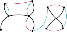
Figure 2. The set of ramification points $\boldsymbol{E}=\{{\boldsymbol{e}}_{0},\ldots,{\boldsymbol{e}}_{9}\}$ of $\boldsymbol{\mathfrak{R}}$ as seen from $D^{(0)}$ and “half ” of the cycle $\boldsymbol{\Delta}$ and the cycles of the homology basis. Due to involution-symmetry, the picture in $D^{(1)}$ is identical. The point where four subarcs of $\Delta$ meet is not a ramification point of $\boldsymbol{\mathfrak{R}}$.

Denote by $\vec{\Omega}:=\left(\Omega_{1},\ldots,\Omega_{g}\right)^{\mathsf{T}}$ the column vector of $g$ linearly independent holomorphic differentials normalized so that $\oint_{\boldsymbol{\upalpha}_{k}}\vec{\Omega}=\vec{e}_{k}$, where $\{\vec{e}_{k}\}_{k=1}^{g}$ is the standard basis for $\mathbb{R}^{g}$ and $\vec{e}^{\mathsf{T}}$ is the transpose of $\vec{e}$. Set

(7) $$\boldsymbol{B}:=\left[\oint_{\boldsymbol{\upbeta}_{j}}\Omega_{k}\right]_{j,k=1}^{g}.$$

It is known that the matrix $\boldsymbol{B}$ is symmetric and has positive definite imaginary part.

A divisor on $\boldsymbol{\mathfrak{R}}$ is a finite linear combination of points from $\boldsymbol{\mathfrak{R}}$ with integer coefficients. The degree of a divisor is the sum of its coefficients. The divisor is called effective if all the coefficients are non-negative. We define Abel’s map on divisors of $\boldsymbol{\mathfrak{R}}$ by

(8) $$\mathfrak{a}\left(\sum n_{j}{\boldsymbol{z}}_{j}\right):=\sum n_{j}\int_{{\boldsymbol{e}}_{0}}^{{\boldsymbol{z}}_{j}}\vec{\Omega}.$$

A divisor $\mathcal{D}=\sum n_{j}{\boldsymbol{z}}_{j}-\sum m_{j}{\boldsymbol{x}}_{j}$, $n_{j},m_{j}>0$, is called principal if there exists a rational function on $\boldsymbol{\mathfrak{R}}$ that has a zero at every ${\boldsymbol{z}}_{j}$ of multiplicity $n_{j}$, a pole at every ${\boldsymbol{x}}_{j}$ of order $m_{j}$, and otherwise is non-vanishing and finite. By Abel’s theorem, $\mathcal{D}$ is principal if and only if its degree is zero and

$$\mathfrak{a}(\mathcal{D})\equiv\vec{0}\quad\big{(}\mathrm{mod~{}periods~{}}\vec{\Omega}\>\big{)},$$

where the equivalence of two vectors $\vec{c},\vec{u}\in\mathbb{C}^{g}$ is defined by $\vec{c}\equiv\vec{u}$ $\big{(}\mathrm{mod~{}periods~{}}\vec{\Omega}\>\big{)}$ if and only if $\vec{c}-\vec{u}=\vec{j}+\boldsymbol{B}\vec{m}$, for some $\vec{j},\vec{m}\in\mathbb{Z}^{g}$.

For any point ${\boldsymbol{v}}\in\boldsymbol{\mathfrak{R}}\setminus\boldsymbol{E}$ there exists a unique differential, say $G_{\boldsymbol{v}}$, such that it is holomorphic on $\boldsymbol{\mathfrak{R}}\setminus\{{\boldsymbol{v}},{\boldsymbol{v}}^{*}\}$, has polar singularities at ${\boldsymbol{v}}$ and ${\boldsymbol{v}}^{*}$ with respective residues $-1$ and $1$, and whose periods are purely imaginary. Given $\mathcal{V}$ as in (5), define vectors $\vec{\omega}_{n}$ and $\vec{\tau}_{n}$ by

(9) $$(\vec{\omega}_{n})_{k}:=-\frac{1}{4\pi\mathrm{i}}\sum_{i=1}^{2n}\oint_{\boldsymbol{\upbeta}_{k}}G_{v_{2n,i}^{(0)}}\quad\text{and}\quad(\vec{\tau}_{n})_{k}:=\frac{1}{4\pi\mathrm{i}}\sum_{i=1}^{2n}\oint_{\boldsymbol{\upalpha}_{k}}G_{v_{2n,i}^{(0)}},$$

where we adopt the notation $(\vec{c})_{k}:=c_{k}$ for $\vec{c}=(c_{1},\ldots,c_{g})$. Notice that these constants are real. Given a continuous function $\rho$ on $\Delta$, we are interested in the solutions of the following Jacobi inversion problem: find an effective divisor $\mathcal{D}_{n}$ of degree $g$ such that

(10) $$\mathfrak{a}(\mathcal{D}_{n})\,\equiv\,\mathfrak{a}\big{(}g\infty^{(1)}\big{)}+\vec{c}_{\rho}+\vec{\omega}_{n}+\boldsymbol{B}\vec{\tau}_{n},\quad\big{(}\mathrm{mod~{}periods~{}}\vec{\Omega}\>\big{)},$$

where $\vec{c}_{\rho}:=\frac{1}{2\pi\mathrm{i}}\oint_{\boldsymbol{\Delta}}\log(\rho\circ\pi)\vec{\Omega}$. This problem is always solvable and the solution is unique up to a principal divisor. That is, if $\mathcal{D}_{n}-\big{\{}\mbox{ principal divisor }\big{\}}$ is an effective divisor, then it also solves (10). Immediately one can see that the subtracted principal divisor should have a positive part of degree at most $g$. As $\boldsymbol{\mathfrak{R}}$ is hyperelliptic, such divisors come solely from rational functions on $\overline{\mathbb{C}}$ lifted to $\boldsymbol{\mathfrak{R}}$. In particular, such principal divisors are involution-symmetric. Hence, if a solution of (10) contains at least one involution-symmetric pair of points, then replacing this pair by another such pair produces a different solution of (10). However, if a solution does not contain such a pair, then it solves (10) uniquely.

Proposition 3.3.

Let $\rho$ be a Hölder continuous and non-vanishing function on $\Delta$. If (10) is uniquely solvable for a given index $n$, then there exists a sectionally meromorphic in $\boldsymbol{\mathfrak{R}}\setminus\boldsymbol{\Delta}$ function $\Psi_{n}$ whose zeros and poles there are described by the divisor

(11) $$(n-g)\infty^{(1)}+\mathcal{D}_{n}-n\infty^{(0)},$$

and whose traces on $\boldsymbol{\Delta}$ are continuous and satisfy

(12) $$\Psi_{n-}({\boldsymbol{x}})=\big{(}\rho(x)/v_{2n}(x)\big{)}\Psi_{n+}({\boldsymbol{x}}),\quad{\boldsymbol{x}}\in\boldsymbol{\Delta}.$$

Moreover, if $\Psi$ is a sectionally meromorphic function in $\boldsymbol{\mathfrak{R}}\setminus\boldsymbol{\Delta}$ satisfying (12) whose divisor has a form $(n-g)\infty^{(1)}+\mathcal{D}-n\infty^{(0)}$ for some effective divisor $\mathcal{D}$, then $\Psi$ is a constant multiple of $\Psi_{n}$.

Together with $\Psi_{n}$ we shall need the following sequence of functions.

Proposition 3.4.

Let an index $n$ be such that (10) is uniquely solvable. If $\mathcal{D}_{n}$ does not contain $\infty^{(0)}$, then there exists a unique, up to a constant factor, rational function $\Upsilon_{n}$ on $\boldsymbol{\mathfrak{R}}$ such that

$$(\Upsilon_{n})+\mathcal{D}_{n}+\infty^{(1)}-\infty^{(0)}$$

is an effective divisor, where $(\Upsilon_{n})$ is the divisor of the zeros and poles of $\Upsilon_{n}$. Moreover, in this case $\Upsilon_{n}$ always has a simple pole at $\infty^{(1)}$.

Effective divisors of degree $g$ can be considered as elements of $\boldsymbol{\mathfrak{R}}^{g}/\Sigma_{g}$, the quotient of $\boldsymbol{\mathfrak{R}}^{g}$ by the symmetric group $\Sigma_{g}$, which is a compact topological space. Thus, it make sense to talk about the limit points of $\{\mathcal{D}_{n}\}$. We shall assume that

Condition 3.1.

There exists an infinite sequence $\mathbb{N}_{*}\subseteq\mathbb{N}$ such that the closure of $\big{\{}\mathcal{D}_{n}\big{\}}_{n\in\mathbb{N}_{*}}$ in the $\boldsymbol{\mathfrak{R}}^{g}/\Sigma_{g}$-topology contains no divisor with an involution-symmetric pair nor with $\infty^{(0)}$.

Observe that (10) is necessarily uniquely solvable for every $n\in\mathbb{N}_{*}$.

Proposition 3.5.

Assume Condition 3.1 is satisfied. Then the functions $\Psi_{n}$ and $\Upsilon_{n}$ can be normalized so that

(13) $$\big{|}\Psi_{n}\big{(}z^{(1)}\big{)}\big{|}^{2},\big{|}(\Psi_{n}\Upsilon_{n})\big{(}z^{(1)}\big{)}\big{|}^{2}\leq C\exp\left\{\sum_{i=0}^{2n}g\big{(}z^{(1)},v_{2n,i}^{(0)}\big{)}\right\}\left|\frac{w^{2}(z)}{v_{2n}(z)}\right|,$$

$\quad n\in\mathbb{N}_{*}$, on any closed set $K\subset D$ for some constant $C=C(K,\mathbb{N}_{*})$.

Recall that according to Definition 3.2(ii) the exponential in the right-hand side of (13) vanishes at every zero of $v_{2n}(z)$ with corresponding multiplicity and their sequence approaches zero locally uniformly in $D$.

Concerning the unique solvability of (10) and the existence of a sequence $\mathbb{N}_{*}$ as in Condition 3.1 nothing is known beyond the special case of the classical diagonal Padé approximants, i.e., when $\mathcal{V}=\mathcal{V}_{\infty}$ [3, 47].

Theorem 3.6 (Aptekarev-Y.).

Assume that $\mathcal{V}=\mathcal{V}_{\infty}$. Let $\mathcal{D}_{n}$ be either the unique solution of (10) or the solution where all involution-symmetric pairs are replaced by $\infty^{(0)}+\infty^{(1)}$. Then

$$\mathcal{D}_{n}=\sum_{i=1}^{g-l}{\boldsymbol{z}}_{i}+k\infty^{(0)}+(l-k)\infty^{(1)}\quad\Leftrightarrow\quad\mathcal{D}_{n+j}=\mathcal{D}_{n}+j\big{(}\infty^{(0)}-\infty^{(1)}\big{)}$$

for $j\in\{-k,\ldots,l-k\}$, where $l>0$, $k\in\{0,\ldots,l\}$, and $|z_{i}|<\infty$. In particular, the subsequence of indices for which (10) is uniquely solvable, say $\mathbb{N}^{\prime}$, cannot have gaps larger than $g-1$. Moreover, let $\mathbb{N}^{\prime\prime}\subset\mathbb{N}^{\prime}$ be a subsequence such that

$$\mathcal{D}_{n}\to\mathcal{D}+\sum_{i=1}^{k}\left(z_{i}^{(0)}+z_{i}^{(1)}\right)+l_{0}\infty^{(0)}+l_{1}\infty^{(1)}\quad\text{as}\quad\mathbb{N}^{\prime\prime}\ni n\to\infty,$$

where an effective divisor $\mathcal{D}$ has degree $g-2k-l_{0}-l_{1}$ and contains neither involution-symmetric pairs, nor $\infty^{(0)}$, nor $\infty^{(1)}$. Then there exists a subsequence $\mathbb{N}^{\prime\prime\prime}$ such that

$$\mathcal{D}_{n-l_{1}-k}\to\mathcal{D}+(l_{0}+l_{1}+2k)\infty^{(1)}\quad\text{as}\quad\mathbb{N}^{\prime\prime\prime}\ni n\to\infty.$$

In particular, one can take $\mathbb{N}_{*}=\mathbb{N}^{\prime\prime\prime}$.

We prove Propositions 3.3–3.5 in Section 5.

3.3. Asymptotics of the Approximants

Given $\Delta$ as in Definition 3.2(i) and a function $\rho$ on $\Delta$, set

(14) $$f_{\rho}(z):=\frac{1}{2\pi\mathrm{i}}\int_{\Delta}\frac{\rho(t)}{t-z}\frac{\mathrm{d}t}{w_{+}(t)},\quad z\in D.$$

We shall be interested in continuous and non-vanishing functions $\rho$ such that a continuous determination of the logarithm $\log\rho$ belongs to the fractional Sobolev space $W^{1-1/p}_{p}$, $p\in(1,\infty)$, that is,

(15) $$\iint_{\Delta\times\Delta}\left|\frac{\log\rho(x)-\log\rho(y)}{x-y}\right|^{p}|\mathrm{d}x||\mathrm{d}y|<\infty.$$

When $p>2$, it follows from Sobolev imbedding theorem that every function in $W^{1-1/p}_{p}$ is in fact Lipschitz continuous with index $1-\frac{2}{p}$. For convenience, we also put

(16) $$\left\{\begin{array}[]{l}\Psi_{n}(z):=\Psi_{n}\big{(}z^{(0)}\big{)},\vskip 6.0pt plus 2.0pt minus 2.0pt\\ \Psi_{n}^{*}(z):=\Psi_{n}\big{(}z^{(1)}\big{)},\end{array}\right.\quad\text{and}\quad\left\{\begin{array}[]{l}\Upsilon_{n}(z):=\Upsilon_{n}\big{(}z^{(0)}\big{)},\vskip 6.0pt plus 2.0pt minus 2.0pt\\ \Upsilon_{n}^{*}(z):=\Upsilon_{n}\big{(}z^{(1)}\big{)},\end{array}\right.$$

$z\in D$, where $\Psi_{n},\Upsilon_{n}$ are the functions from Propositions 3.3–3.5. Then the following theorem holds.

Theorem 3.7.

Given $\boldsymbol{\mathfrak{R}}$ and $\mathcal{V}$ as in (3) and (5), assume that $\Delta$ is symmetric with respect to $(\boldsymbol{\mathfrak{R}},\mathcal{V})$ in the sense of Definition 3.2. Let $\rho$ be a non-vanishing function on $\Delta$ with $\log\rho\in W_{p}^{1-1/p}$ for some $p>4$ and let $f_{\rho}$ be as in (14). Further, let

$$p_{n}/q_{n}:=[n/n;V_{2n}]_{f_{\rho}}\quad\text{and}\quad R_{n}:=R_{n,n}$$

be the diagonal multipoint Padé approximant to $f_{\rho}$ associated with $V_{2n}$ and its linearized error function, see Definition 2.1. Assuming that the interpolation scheme $\mathcal{V}$ is such that Condition 3.1 is fulfilled, it holds for all $n\in\mathbb{N}_{*}$ large enough that

(17) $$\left\{\begin{array}[]{rll}q_{n}&=&\displaystyle\gamma_{n}\Psi_{n}\left(1+\varepsilon_{n1}+\varepsilon_{n2}\Upsilon_{n}\right),\vskip 12.0pt plus 4.0pt minus 4.0pt\\ wR_{n}&=&\displaystyle\gamma_{n}\Psi_{n}^{*}\left(1+\varepsilon_{n1}+\varepsilon_{n2}\Upsilon_{n}^{*}\right),\end{array}\right.$$

where $\varepsilon_{nj}(\infty)=0$, $\varepsilon_{nj}=o(1)$ with respect to $n$ and locally uniformly in $D$, and $\gamma_{n}$ is a normalizing constant such that $\gamma_{n}\Psi_{n}(z)=z^{n}(1+o(1))$ as $z\to\infty$.

In the case of classical Padé approximants Theorem 3.7 should be compared to results by Szegő [43] ($\Delta=[-1,1]$ and $\rho(t)\mathrm{d}t/w_{+}(t)$ is replaced by any positive measure satisfying Szegő’s condition); Nuttall [27] ($\Delta=[-1,1]$ and $\rho$ is Hölder continuous); Suetin [42] ($\Delta$ is a union of disjoint analytic arcs and $\rho$ is Hölder continuous); Baratchart and the author [11] ($\Delta$ consists of three arcs meeting at a common point and $\rho$ is Dini continuous); Aptekarev and the author [3] ($\Delta$ is such that no endpoint has bifurcation index more than $3$, $\rho$ is holomorphic across each $\Delta_{j}$ and can have power-type singularities at endpoints with bifurcation index $1$); and the author [47] ($\Delta$ is any and $\rho$ is holomorphic around each connected component of $\Delta$). Of course, in all the cases $\Delta$ is a symmetric contour and $\rho(t)$ is non-vanishing (except for Szegő’s result).

In the case of multipoint Padé approximants Theorem 3.7 is an addition to the results by de la Calle Ysern and López Lagomasino [14] (Szegő’s set up with interpolation schemes as in the present study plus additional conjugate-symmetry); Baratchart and the author [9, 10] ($\Delta$ is a single arc and $\rho$ is Dini-continuous in [9] and with power-type singularities at the endpoints while satisfying Sobolev-type condition that depends on the magnitude of the singularities on $\Delta^{\circ}$ in [10], the class of interpolation schemes is more restricted in [10] while in [9] they are exactly the same as in the present paper); Aptekarev [2] (it is a more general result on varying non-Hermitian orthogonality that can be applied to multipoint Padé approximants to yield the results of [9, 10], which came later, for holomorphic $\rho$).

We prove Theorem 3.7 in Section 6.

3.4. Numerical Simulations

The following computations were performed in MAPLE 18 software using 64 digit precision.

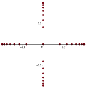
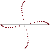
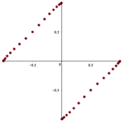
Figure 3. Poles of multipoint Padé approximants to $(z^{4}-1)^{-1/2}$ associated with interpolation schemes $\mathcal{V}_{*}$, $\mathcal{V}_{*}^{\prime}$, and $\mathcal{V}_{*}^{\prime\prime}$.

Let $f(z)=(z^{4}-1)^{-1/2}$. The symmetry of $f(z)$ readily implies that the Stahl’s contour $\Delta_{f}=\Delta_{\infty}$ from Theorem 2.1 is equal to $[-1,1]\cup[-\mathrm{i},\mathrm{i}]$. The corresponding surface from (3) is given by $\boldsymbol{\mathfrak{R}}_{*}:=\big{\{}(z,w):~{}w^{2}=z^{4}-1\big{\}}$. Similar symmetry considerations also yield that for the interpolation scheme $\mathcal{V}_{*}$ such that $V_{4n+2}=V_{4n}\cup\{\infty,\infty\}$ and

$$V_{4n}=\left\{\underbrace{1+\mathrm{i},\ldots,1+\mathrm{i}}_{n~{}\text{times}},\underbrace{-1+\mathrm{i},\ldots,-1+\mathrm{i}}_{n~{}\text{times}},\underbrace{-1-\mathrm{i},\ldots,-1-\mathrm{i}}_{n~{}\text{times}},\underbrace{1-\mathrm{i},\ldots,1-\mathrm{i}}_{n~{}\text{times}}\right\},$$

$[-1,1]\cup[-\mathrm{i},\mathrm{i}]$ remains symmetric with respect to $(\boldsymbol{\mathfrak{R}}_{*},\mathcal{V}_{*})$. The poles of $[34/34;V_{68}]_{f}$ are shown on Figure 3(a). If we take now $V_{4n+2}^{\prime}=V_{4n}^{\prime}\cup\{\infty,\infty\}$ and

$$V_{4n}^{\prime}=\left\{\underbrace{\frac{1}{4}+\mathrm{i},\ldots,\frac{1}{4}+\mathrm{i}}_{n~{}\text{times}},\underbrace{-1+\frac{\mathrm{i}}{4},\ldots,-1+\frac{\mathrm{i}}{4}}_{n~{}\text{times}},\underbrace{-\frac{1}{4}-\mathrm{i},\ldots,-\frac{1}{4}-\mathrm{i}}_{n~{}\text{times}},\underbrace{1-\frac{\mathrm{i}}{4},\ldots,1-\frac{\mathrm{i}}{4}}_{n~{}\text{times}}\right\},$$

then the poles of $[60/60;V_{120}^{\prime}]_{f}$ are shown on Figure 3(b). The Riemann surfaces needed to analyze these approximants is still $\boldsymbol{\mathfrak{R}}_{*}$ and the contour symmetric with respect to $(\boldsymbol{\mathfrak{R}},\mathcal{V}_{*}^{\prime})$ can be obtained via the process described in Theorem 3.2. If we take

$$V_{2n}^{\prime\prime}=\left\{\underbrace{1+\mathrm{i},\ldots,1+\mathrm{i}}_{n~{}\text{times}},\underbrace{-1-\mathrm{i},\ldots,-1-\mathrm{i}}_{n~{}\text{times}}\right\},$$

then the poles of $[34/34;V_{68}^{\prime\prime}]_{f}$ are shown on Figure 3(c). As in the previous case, $\boldsymbol{\mathfrak{R}}_{*}$ is still the appropriate Riemann surface, but the contour symmetric with respect to $(\boldsymbol{\mathfrak{R}}_{*},\mathcal{V}_{*}^{\prime\prime})$ cannot be obtained via the procedure of Theorem 3.2. It is most likely that a version of Theorem 3.2 where the map $\Xi$ is defined on the surface itself, could prove the existence of such a contour.

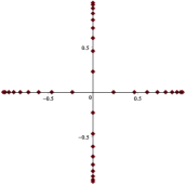
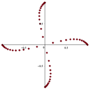
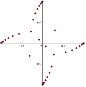
Figure 4. Poles of multipoint Padé approximants to $(z^{4}-1)^{-1/4}$ associated with interpolation schemes $\mathcal{V}_{*}$, $\mathcal{V}_{*}^{\prime}$, and $\mathcal{V}_{*}^{\prime\prime}$.

Let now $g(z)=(z^{4}-1)^{-1/4}$. Again, we have that $\Delta_{g}=\Delta_{\infty}=[-1,1]\cup[-\mathrm{i},\mathrm{i}]$. Thus, if we use the interpolation scheme $\mathcal{V}_{*}$, the poles of the corresponding multipoint Padé approximants must accumulate on $[-1,1]\cup[-\mathrm{i},\mathrm{i}]$, see Figure 4(a) for the poles of $[36/36;V_{72}]_{g}$. Likewise, the poles of $[n/n;V_{2n}^{\prime}]_{g}$ and of $[n/n;V_{2n}^{\prime}]_{f}$ accumulate on the same contour, see Figure 4(b) for the poles of $[60/60;V_{120}^{\prime}]_{g}$. However, the conjectural contour symmetric with respect to $(\boldsymbol{\mathfrak{R}}_{*},V_{*}^{\prime\prime})$ does not make $g$ single-valued in its complement. That is, the surface $\boldsymbol{\mathfrak{R}}_{*}$ is no longer appropriate for the considered approximation problem. On Figure 4(c) the poles of $[34/34;V_{68}^{\prime\prime}]_{g}$ are depicted. It suggests that the appropriate surface should be given by $\big{\{}(z,w):~{}w^{2}=(z^{2}-b^{2})(z^{4}-1)\big{\}}$ for some unique $b$. The genus of this surface is 2 and one can clearly see two poles with atypical behavior on Figure 4(c).

4. Symmetric Contours

The following observation will be important: if $L$ is a smooth arc and $g(z)$ is harmonic from each side of $L$, $g(s)=0$ for $s\in L$, and

(18) $$\frac{\partial g}{\partial\boldsymbol{n}_{-}}=\frac{\partial g}{\partial\boldsymbol{n}_{+}}\quad\text{on}\quad L^{\circ},$$

where $L^{\circ}$ is $L$ without the endpoints, then the harmonic continuation of $g(z)$ across $L^{\circ}$ is given by $-g(z)$. Indeed, let $H:=\partial_{z}g$, where $2\partial_{z}:=\partial_{x}-\mathrm{i}\partial_{y}$. Then $H(z)$ is a holomorphic function from each side of $L$. Denote by $\boldsymbol{\tau}(s)$ and $\boldsymbol{n}_{\pm}(s)$ the unit tangent vector and the one-sided unit normal vectors to $L^{\circ}$ at $s\in L^{\circ}$. Further, put $\tau(s)$ and $n_{\pm}(s)$ to be the corresponding unimodular complex numbers, $n_{+}(s)=\mathrm{i}\tau(s)$. Then

$$0=\frac{\partial g}{\partial\boldsymbol{\tau}}(s)=\big{\langle}\nabla g(s),\boldsymbol{\tau}(s)\big{\rangle}=\mp 2\mathsf{Im}\big{(}n_{\pm}(s)H_{\pm}(s)\big{)}\quad\Rightarrow\\ \frac{\partial g}{\partial\boldsymbol{n}_{\pm}}(s)=\big{\langle}\nabla g(s),\boldsymbol{n}_{\pm}(s)\big{\rangle}=2\mathsf{Re}\big{(}n_{\pm}(s)H_{\pm}(s)\big{)}=n_{\pm}(s)H_{\pm}(s).$$

As $n_{+}(s)=-n_{-}(s)$, $-H(z)$ is the analytic continuation of $H(z)$ across $L^{\circ}$, which is equivalent to the original claim.

4.1. Proof of Proposition 3.1

It follows from Theorem 2.1 that $\Delta_{f}$ is a branch cut for $h_{D_{f}}(z)$ and the jump of $h_{D_{f}}(z)$ across any subarc of $\Delta_{f}$ is non-zero. According to the choice of the set $E$, $\boldsymbol{\mathfrak{R}}$ is also the Riemann surface of $h_{D_{f}}(z)$. Therefore, $\Delta_{f}$ satisfies Definition 3.2(i). Realize $\boldsymbol{\mathfrak{R}}$ as in (6) with $\Delta$ and $D$ replaced by $\Delta_{f}$ and $D_{f}$. Define $g({\boldsymbol{z}})$ on $\boldsymbol{\mathfrak{R}}$ by lifting $(-1)^{i}g_{D_{f}}(z)$ to $D^{(i)}$ and extend it to $\boldsymbol{\Delta}$ continuously by zero. Zeroing on $\boldsymbol{\Delta}$, the S-property from Theorem 2.1(iii), and (18) imply that $g({\boldsymbol{z}})$ is harmonic across $\boldsymbol{\Delta}$. Since only constants are harmonic on the entire surface $\boldsymbol{\mathfrak{R}}$, $g({\boldsymbol{z}})=g({\boldsymbol{z}},\infty^{(0)})$ and Definition 3.2(ii) follows.

To prove the second claim of the proposition, define $\nu_{n}$ as in (2). Realize $\boldsymbol{\mathfrak{R}}$ as in (6). Define $g_{\nu_{n}}({\boldsymbol{z}})$ on $\boldsymbol{\mathfrak{R}}$ by lifting $(-1)^{i}g_{D}^{\nu_{n}}(z)$ to $D^{(i)}$ and then extending it to $\boldsymbol{\Delta}$ by continuity. It follows from the definition of the Green functions and Definition 3.1 that

$$g_{\nu_{n}}({\boldsymbol{z}})-g_{n}({\boldsymbol{z}}),\quad g_{n}({\boldsymbol{z}}):=\frac{1}{2n}\sum_{v\in V_{2n}}g\big{(}{\boldsymbol{z}},v^{(0)}\big{)},$$

is harmonic in each domain $D^{(i)}$. Moreover, as $g_{\nu_{n}}\equiv 0$ on $\boldsymbol{\Delta}$ and $g_{n}=o(1)$ by Definition 3.2(ii), the above differences converge to zero uniformly on $\boldsymbol{\mathfrak{R}}$ by the maximum principle for harmonic functions. In another connection, let $O$ be a neighborhood of $\Delta$ such that $O\cap V_{2n}=\varnothing$ for all $n$. Then $g_{D}^{\nu_{n}}(z)$ and $g_{D}^{\nu}(z)$ are harmonic in $O\setminus\Delta$. This and the weak^∗ convergence imply that the functions $g_{D}^{\nu_{n}}(z)$ converge to $g_{D}^{\nu}(z)$ locally uniformly in $O$. Define $g({\boldsymbol{z}})$ by lifting $(-1)^{i}g_{D}^{\nu}(z)$ to $D^{(i)}$. The previous two limits yield that $g({\boldsymbol{z}})=g_{n}({\boldsymbol{z}})+o(1)$, where $o(1)$ holds locally uniformly in $\pi^{-1}(O)$. As the functions $g_{n}({\boldsymbol{z}})$ are harmonic in $\pi^{-1}(O)$, so must be their uniform limit. This and claim (18) finish the proof of the proposition.

4.2. Functions $g({\boldsymbol{z}},{\boldsymbol{v}})$

The main goal of this subsection is to show that

(19) $$g({\boldsymbol{z}},{\boldsymbol{v}})=g({\boldsymbol{v}},{\boldsymbol{z}}).$$

To this end, let us point out that the contour $\Delta_{v}$ always exists (this is the first claim of Theorem 3.2). Indeed, let $\boldsymbol{\Delta}_{\boldsymbol{v}}$ be the zero level line of $g(\cdot,{\boldsymbol{v}})$. Since the function $g({\boldsymbol{z}},{\boldsymbol{v}})$ approaches $+\infty$ as ${\boldsymbol{z}}\to{\boldsymbol{v}}$, approaches $-\infty$ as ${\boldsymbol{z}}\to{\boldsymbol{v}}^{*}$, and is harmonic on $\boldsymbol{\mathfrak{R}}\setminus\{{\boldsymbol{v}},{\boldsymbol{v}}^{*}\}$, $\boldsymbol{\Delta}_{\boldsymbol{v}}$ separates $\boldsymbol{\mathfrak{R}}$ into exactly two connected components. Symmetry (4) then yields that $\boldsymbol{\Delta}_{\boldsymbol{v}}$ is involution-symmetric and the involution $\cdot^{*}$ sends one component of $\boldsymbol{\mathfrak{R}}\setminus\boldsymbol{\Delta}_{\boldsymbol{v}}$ into another. It only remains to notice that $\Delta_{v}=\pi(\boldsymbol{\Delta}_{\boldsymbol{v}})$.

Fix ${\boldsymbol{z}}$ and ${\boldsymbol{v}}$. Realize $\boldsymbol{\mathfrak{R}}$ as in (6) with $\Delta$ and $D$ replaced by $\Delta_{v}$ and $D_{v}:=\overline{\mathbb{C}}\setminus\Delta_{v}$. Assume first that ${\boldsymbol{z}}$ belongs to the same component of $\boldsymbol{\mathfrak{R}}\setminus\boldsymbol{\Delta}_{\boldsymbol{v}}$ as ${\boldsymbol{v}}$, say $D^{(0)}$. Then it easily follows from the properties of the Green function that

(20) $$g\big{(}s^{(0)},v^{(0)}\big{)}=g_{D_{v}}(s,v),\quad s\in D_{v}.$$

Denote by $\partial D_{v}$ the boundary of $D_{v}$ considered as a set of different accessible points from $D_{v}$. Hence, every smooth point of $\Delta_{v}$ appears twice in $\partial D_{v}$ since it can be accessed from one side of the corresponding subarc of $\Delta_{v}$ or the other. Let $\big{\{}\widehat{\delta}_{s}\big{\}}_{s\in D_{v}}$ be the harmonic measure on $\partial D_{v}$ (equivalently, $\widehat{\delta}_{s}$ is the balayage of the Dirac delta distribution $\delta(s)$ from $D_{v}$ onto $\partial D_{v}$, see [35, Section II.4]). Then it holds that

$$g\big{(}s^{(0)},{\boldsymbol{z}}\big{)} = g_{D_{v}}(s,z)+\left(g\big{(}s^{(0)},{\boldsymbol{z}}\big{)}-g_{D}(s,z)\right)$$

$$= g_{D_{v}}(s,z)+\int_{\partial D_{v}}\left(g\big{(}t^{(0)},{\boldsymbol{z}}\big{)}-g_{D}(t,z)\right)\mathrm{d}\widehat{\delta}_{s}(t)$$

by the properties of harmonic measure. Moreover, since Green function is zero on the boundary of the domain, we get that

$$g\big{(}s^{(0)},{\boldsymbol{z}}\big{)} = g_{D_{v}}(s,z)+\int_{\partial D_{v}}g\big{(}t^{(0)},{\boldsymbol{z}}\big{)}\mathrm{d}\widehat{\delta}_{s}(t)$$

$$= g_{D_{v}}(s,z)+\frac{1}{2\pi}\int_{\partial D_{v}}g\big{(}t^{(0)},{\boldsymbol{z}}\big{)}\frac{\partial g_{D_{v}}(\cdot,s)}{\partial\boldsymbol{n}}\big{|}_{t}\mathrm{d}t,$$

where $\partial/\partial\boldsymbol{n}$ is the partial derivative with respect to the inner normal on $\partial D_{v}$ and the second equality follows from [35, Equation (II.4.32) and Theorem II.1.5]. Equivalently, using the one-sided normals $\boldsymbol{n}_{\pm}$ on $\Delta_{v}$, we can write

$$g\big{(}s^{(0)},{\boldsymbol{z}}\big{)} = g_{D_{v}}(s,z)+\frac{1}{2\pi}\int_{\Delta_{v}}\left(g_{+}\big{(}t^{(0)},{\boldsymbol{z}}\big{)}\frac{\partial g_{D_{v}}(\cdot,s)}{\partial\boldsymbol{n}_{+}}\big{|}_{t}+g_{-}\big{(}t^{(0)},{\boldsymbol{z}}\big{)}\frac{\partial g_{D_{v}}(\cdot,s)}{\partial\boldsymbol{n}_{-}}\big{|}_{t}\right)\mathrm{d}t$$

$$= g_{D_{v}}(s,z)+\frac{1}{2\pi}\int_{\Delta_{v}}\left(\frac{\partial g_{D_{v}}(\cdot,s)}{\partial\boldsymbol{n}_{+}}\big{|}_{t}-\frac{\partial g_{D_{v}}(\cdot,s)}{\partial\boldsymbol{n}_{-}}\big{|}_{t}\right)g_{+}\big{(}t^{(0)},{\boldsymbol{z}}\big{)}\mathrm{d}t,$$

where the second equality follows from (4). When ${\boldsymbol{s}}={\boldsymbol{v}}$, the last integral is equal to zero by claim (18) and the very definition of $\Delta_{v}$. Hence,

(21) $$g\big{(}v^{(0)},z^{(0)}\big{)}=g_{D_{v}}(v,z)$$

and the desired symmetry (19) follows from (20), (21), and the well known symmetry of the Green function, see [35, Theorem II.4.9]. The cases when ${\boldsymbol{z}}$ and ${\boldsymbol{v}}$ belong to different connected components of $\boldsymbol{\mathfrak{R}}\setminus\boldsymbol{\Delta}_{\boldsymbol{v}}$ or ${\boldsymbol{z}}\in\Delta_{\boldsymbol{v}}$, can be shown similarly.

One consequence of (19) is that $g({\boldsymbol{z}},{\boldsymbol{v}})$ is a harmonic function of ${\boldsymbol{v}}\in\boldsymbol{\mathfrak{R}}\setminus\{{\boldsymbol{z}},{\boldsymbol{z}}^{*}\}$. Therefore, if $\boldsymbol{\mathfrak{R}}$ is realized as in (6), then for any closed set $K\subset D$ there exists a constant $C_{K}$ such that

(22) $$\big{|}g\big{(}{\boldsymbol{x}},v_{1}^{(0)}\big{)}-g\big{(}{\boldsymbol{x}},v_{2}^{(0)}\big{)}\big{|}\leq C_{K}|v_{1}-v_{2}|,\quad{\boldsymbol{x}}\in\boldsymbol{\Delta},\quad v_{1},v_{2}\in K.$$

4.3. Proof of Theorem 3.2

The existence of $\Delta_{v}$ was shown in the previous subsection. Thus, we only need to prove the second claim of the theorem. Set

$$\Delta_{\Xi}:=\Xi(\Delta)\quad\text{and}\quad D_{\Xi}:=\overline{\mathbb{C}}\setminus\Delta_{\Xi},$$

and realize $\boldsymbol{\mathfrak{R}}$ as in (6) with $\Delta$ replaced by $\Delta_{\Xi}$. Denote by $O$ the interior domain of $\Xi(L_{c})$. Define

$$g\big{(}z^{(i)}\big{)}=(-1)^{i}g_{D_{v}}\big{(}\Xi^{-1}(z),v\big{)},\quad z\in O,$$

where $g_{D_{v}}(z,v)$ is the Green function with pole at $v$ for $D_{v}$. Then, as in the proof of Proposition 3.1, $g({\boldsymbol{z}})$ is harmonic in $\pi^{-1}(O)$ and $\pi^{-1}(L_{c})$ necessarily consists of two level lines of $g({\boldsymbol{z}})$. Assume that we can write

(23) $$g({\boldsymbol{z}})=\int_{\partial O}g({\boldsymbol{z}},s)\frac{\partial g}{\partial\boldsymbol{n}}(s)|\mathrm{d}s|,\quad{\boldsymbol{z}}\in\pi^{-1}(O),$$

where we adopt the convention $f(z):=f\big{(}z^{(0)}\big{)}$ and $f^{*}(z):=f\big{(}z^{(1)}\big{)}$, $z\in D_{\Xi}$, for a function $f({\boldsymbol{z}})$ on $\boldsymbol{\mathfrak{R}}$. Split $\partial O$ into $2n$ disjoint (except for the endpoints) subarcs $L_{2n,i}$ such that

$$\int_{L_{2n,i}}\frac{\partial g}{\partial\boldsymbol{n}}(s)|\mathrm{d}s|=\frac{1}{2n}\int_{\partial O}\frac{\partial g}{\partial\boldsymbol{n}}(s)|\mathrm{d}s|=:\frac{1}{2nC}$$

and pick $v_{2n,i}\in L_{2n,i}$. Since $g({\boldsymbol{x}})=0$ for ${\boldsymbol{x}}\in\boldsymbol{\Delta}$, we get from (23) that

$$g_{n}({\boldsymbol{x}}):=\sum_{i=1}^{2n}g\big{(}{\boldsymbol{x}},v_{2n,i}^{(0)}\big{)}=2nC\sum_{i=1}^{2n}\int_{L_{2n,i}}g\big{(}{\boldsymbol{x}},v_{2n,i}^{(0)}\big{)}\frac{\partial g}{\partial\boldsymbol{n}}(v)|\mathrm{d}v|=\\ =2nC\sum_{i=1}^{2n}\int_{L_{2n,i}}\left(g\big{(}{\boldsymbol{x}},v_{2n,i}^{(0)}\big{)}-g({\boldsymbol{x}},v)\right)\frac{\partial g}{\partial\boldsymbol{n}}(v)|\mathrm{d}v|.$$

Hence, it holds that

(24) $$|g_{n}({\boldsymbol{x}})| \leq 2nC\left(\int_{L}\left|\frac{\partial g}{\partial\boldsymbol{n}}(v)\right||\mathrm{d}v|\right)\max_{i}\max_{v_{1},v_{2}\in L_{2n,i}}\left|g\big{(}{\boldsymbol{x}},v_{1}^{(0)}\big{)}-g\big{(}{\boldsymbol{x}},v_{2}^{(0)}\big{)}\right|,$$

$$\leq C^{\prime}n\max_{i}\mathsf{diam}(L_{2n,i})\leq C^{\prime\prime},\quad{\boldsymbol{x}}\in\boldsymbol{\Delta},$$

by (22) for some constants $C^{\prime},C^{\prime\prime}$ that depend only on $\Xi$. Define $\nu_{n}$ as in (2) with just selected sets $V_{2n}=\{v_{2n,i}\}_{i=1}^{2n}$. The functions

(25) $$g_{n}\big{(}z^{(1)}\big{)}+2ng_{D_{\Xi}}^{\nu_{n}}(z)$$

are harmonic in $D_{\Xi}$ and have bounded traces on $\Delta_{\Xi}$ according to (24). By the maximum principle for harmonic functions they are uniformly bounded above and below in $D_{\Xi}$. As the measures $\nu_{n}$ are supported on $\partial O$, which is compact, any sequence of them contains a weak^∗ convergent subsequence by Helly’s selection principle. Let $\nu$ be the limit. Then

$$g_{D_{\Xi}}^{\nu_{n}}(z)\to g_{D_{\Xi}}^{\nu}(z)\quad\text{as}\quad n\to\infty,\quad z\in D_{\Xi}\setminus\partial O.$$

As $g_{D_{\Xi}}^{\nu}(z)>0$ in $D_{\Xi}$, $g\big{(}z^{(1)}\big{)}\to-\infty$ for every $z\in D_{\Xi}\setminus\partial O$ by the conclusion after (25). Therefore $g\big{(}z^{(1)}\big{)}\to-\infty$ locally uniformly in $D_{\Xi}$ by the maximum principle for subharmonic functions. This shows that the condition in Definition 3.2(ii) is fulfilled and thus finishes the proof of the theorem given representation (23).

To prove (23), let us recall the Green’s formula stated in a form convenient for our purposes. Let $U$ be an open set with piecewise smooth boundary and let $a,b$ be two harmonic functions in $U$ with piecewise smooth traces on $\partial U$. Then

(26) $$\int_{\partial U}a(s)\frac{\partial b}{\partial\boldsymbol{n}}(s)|\mathrm{d}s|=\int_{\partial U}b(s)\frac{\partial a}{\partial\boldsymbol{n}}(s)|\mathrm{d}s|,$$

where $\partial/\partial\boldsymbol{n}$ is the partial derivative with respect to the inner normal on $\partial U$ and $|\mathrm{d}s|$ is the arclength differential.

Given distinct ${\boldsymbol{x}},{\boldsymbol{y}}\in\boldsymbol{\mathfrak{R}}\setminus\{{\boldsymbol{e}}_{0}\}$, denote by $g(\cdot,{\boldsymbol{x}},{\boldsymbol{y}})$ a function that is harmonic in $\boldsymbol{\mathfrak{R}}\setminus\{{\boldsymbol{x}},{\boldsymbol{y}}\}$, normalized so that $g({\boldsymbol{e}}_{0},{\boldsymbol{x}},{\boldsymbol{y}})=0$, and such that

$$g({\boldsymbol{z}},{\boldsymbol{x}},{\boldsymbol{y}})+\left\{\begin{array}[]{rl}\log|z-x|,&|x|<\infty,\vskip 3.0pt plus 1.0pt minus 1.0pt\\ -\log|z|,&x=\infty,\end{array}\right.\quad\text{and}\quad g({\boldsymbol{z}},{\boldsymbol{x}},{\boldsymbol{y}})-\left\{\begin{array}[]{rl}\log|z-y|,&|y|<\infty,\vskip 3.0pt plus 1.0pt minus 1.0pt\\ -\log|z|,&y=\infty,\end{array}\right.$$

are harmonic around ${\boldsymbol{x}}$ and ${\boldsymbol{y}}$, respectively. Existence of such functions follows from the same principles as the existence of $g({\boldsymbol{z}},{\boldsymbol{v}})$ in Definition 3.1. Fix ${\boldsymbol{z}}\in\pi^{-1}(O)\setminus\boldsymbol{\Delta}$ and denote by $U$ a disk centered at $z$ of radius $\delta>0$ small enough so that $\overline{U}\subset O\setminus\Delta_{\Xi}$. Then, assuming ${\boldsymbol{z}}\in D^{(0)}$, it holds that

$$I := \int_{\partial(O\setminus\overline{U})}g(s)\frac{\partial}{\partial\boldsymbol{n}}g\big{(}s,{\boldsymbol{z}},\infty^{(1)}\big{)}|\mathrm{d}s|+\int_{\partial O}g^{*}(s)\frac{\partial}{\partial\boldsymbol{n}}g^{*}\big{(}s,{\boldsymbol{z}},\infty^{(1)}\big{)}|\mathrm{d}s|$$

$$= c\int_{\partial O}\frac{\partial}{\partial\boldsymbol{n}}g\big{(}s,{\boldsymbol{z}},\infty^{(1)}\big{)}|\mathrm{d}s|-c\int_{\partial O}\frac{\partial}{\partial\boldsymbol{n}}g^{*}\big{(}s,{\boldsymbol{z}},\infty^{(1)}\big{)}|\mathrm{d}s|-\int_{\partial U}g(s)\frac{\partial}{\partial\boldsymbol{n}}g\big{(}s,{\boldsymbol{z}},\infty^{(1)}\big{)}|\mathrm{d}s|.$$

Observe that $g\big{(}\cdot,{\boldsymbol{z}},\infty^{(1)}\big{)}$ is harmonic outside of $\overline{O}$ and therefore

$$\int_{\partial O}\frac{\partial}{\partial\boldsymbol{n}}g\big{(}s,{\boldsymbol{z}},\infty^{(1)}\big{)}|\mathrm{d}s|=0$$

by (26). Analogously, (26) and the definition of $g(\cdot,{\boldsymbol{x}},{\boldsymbol{y}})$ yield that

$$\int_{\partial O}\frac{\partial}{\partial\boldsymbol{n}}g^{*}\big{(}s,{\boldsymbol{z}},\infty^{(1)}\big{)}\mathrm{d}s=-\int_{\partial O}\frac{\partial}{\partial\boldsymbol{n}}\log|s||\mathrm{d}s|=\int_{|s|=r}\frac{\partial}{\partial r}\log r|\mathrm{d}s|=2\pi.$$

for any $r$ large. Furthermore, we have

$$\int_{\partial U}g(s)\frac{\partial}{\partial\boldsymbol{n}}g\big{(}s,{\boldsymbol{z}},\infty^{(1)}\big{)}|\mathrm{d}s|=:I_{*}-\int_{\partial U}g(s)\frac{\partial}{\partial\boldsymbol{n}}\log|s-z||\mathrm{d}s|=I_{*}-\frac{1}{\delta}\int_{\partial U}g(s)|\mathrm{d}s|.$$

Thus, we get from the mean-value property of harmonic functions that

(27) $$I=-2\pi c+g({\boldsymbol{z}})-I_{*}.$$

In another connection, since $g({\boldsymbol{x}})=0$ for ${\boldsymbol{x}}\in\boldsymbol{\Delta}$, we deduce from (26) that

$$I := \int_{\partial(O\setminus(\overline{U}\cup\Delta_{\Xi}))}g(s)\frac{\partial}{\partial\boldsymbol{n}}g\big{(}s,{\boldsymbol{z}},\infty^{(1)}\big{)}|\mathrm{d}s|+\int_{\partial(O\setminus\Delta_{\Xi})}g^{*}(s)\frac{\partial}{\partial\boldsymbol{n}}g^{*}\big{(}s,{\boldsymbol{z}},\infty^{(1)}\big{)}|\mathrm{d}s|$$

$$= \int_{\partial(O\setminus(\overline{U}\cup\Delta_{\Xi}))}g\big{(}s,{\boldsymbol{z}},\infty^{(1)}\big{)}\frac{\partial g}{\partial\boldsymbol{n}}(s)|\mathrm{d}s|+\int_{\partial(O\setminus\Delta_{\Xi})}g^{*}\big{(}s,{\boldsymbol{z}},\infty^{(1)}\big{)}\frac{\partial g^{*}}{\partial\boldsymbol{n}}(s)|\mathrm{d}s|$$

$$= \int_{\partial O}\left(g\big{(}s,{\boldsymbol{z}},\infty^{(1)}\big{)}-g^{*}\big{(}s,{\boldsymbol{z}},\infty^{(1)}\big{)}\right)\frac{\partial g}{\partial\boldsymbol{n}}(s)|\mathrm{d}s|-\int_{\partial U}g\big{(}s,{\boldsymbol{z}},\infty^{(1)}\big{)}\frac{\partial g}{\partial\boldsymbol{n}}(s)|\mathrm{d}s|,$$

where we also used the fact that $g\big{(}s,{\boldsymbol{z}},\infty^{(1)}\big{)}=g^{*}\big{(}s,{\boldsymbol{z}},\infty^{(1)}\big{)}$ for $s\in\Delta_{\Xi}$ while $g(z)=-g^{*}(z)$. Clearly, it holds that

$$g\big{(}s,{\boldsymbol{z}},\infty^{(1)}\big{)}-g^{*}\big{(}s,{\boldsymbol{z}},\infty^{(1)}\big{)}=g(s,{\boldsymbol{z}})+g\big{(}s,\infty^{(0)}\big{)}=g({\boldsymbol{z}},s)+g\big{(}s,\infty^{(0)}\big{)}$$

by (19). Using (4) and the symmetry of $g({\boldsymbol{z}})$, we get that

$$\int_{\partial O}g\big{(}s,\infty^{(0)}\big{)}\frac{\partial g}{\partial\boldsymbol{n}}(s)|\mathrm{d}s| = \frac{1}{2}\int_{\partial O}\left(g\big{(}s,\infty^{(0)}\big{)}\frac{\partial g}{\partial\boldsymbol{n}}(s)+g^{*}\big{(}s,\infty^{(0)}\big{)}\frac{\partial g^{*}}{\partial\boldsymbol{n}}(s)\right)|\mathrm{d}s|$$

$$= \frac{1}{2}\int_{\partial(O\setminus\Delta_{\Xi})}\left(g\big{(}s,\infty^{(0)}\big{)}\frac{\partial g}{\partial\boldsymbol{n}}(s)+g^{*}\big{(}s,\infty^{(0)}\big{)}\frac{\partial g^{*}}{\partial\boldsymbol{n}}(s)\right)|\mathrm{d}s|.$$

Then, it follows from (26) that

$$\int_{\partial O}g\big{(}s,\infty^{(0)}\big{)}\frac{\partial g}{\partial\boldsymbol{n}}(s)|\mathrm{d}s| = \frac{1}{2}\int_{\partial(O\setminus\Delta_{\Xi})}\left(g(s)\frac{\partial}{\partial\boldsymbol{n}}g\big{(}s,\infty^{(0)}\big{)}+g^{*}(s)\frac{\partial}{\partial\boldsymbol{n}}g^{*}\big{(}s,\infty^{(0)}\big{)}\right)|\mathrm{d}s|$$

$$= \frac{c}{2}\int_{\partial O}\left(\frac{\partial}{\partial\boldsymbol{n}}g\big{(}s,\infty^{(0)}\big{)}-\frac{\partial}{\partial\boldsymbol{n}}g^{*}\big{(}s,\infty^{(0)}\big{)}\right)|\mathrm{d}s|$$

$$= c\int_{\partial O}\frac{\partial}{\partial\boldsymbol{n}}\log|s||\mathrm{d}s|=-2\pi c.$$

Moreover, it holds that

$$\int_{\partial U}g\big{(}s,{\boldsymbol{z}},\infty^{(1)}\big{)}\frac{\partial g}{\partial\boldsymbol{n}}(s)|\mathrm{d}s|=-\log\delta\int_{\partial U}\frac{\partial g}{\partial\boldsymbol{n}}(s)|\mathrm{d}s|+\\ \int_{\partial U}\left(g\big{(}s,{\boldsymbol{z}},\infty^{(1)}\big{)}+\log|s-z|\right)\frac{\partial g}{\partial\boldsymbol{n}}(s)|\mathrm{d}s|=I_{*},$$

again by (26). Altogether, we have showed that

(28) $$I=\int_{\partial O}g({\boldsymbol{z}},s)\frac{\partial g}{\partial\boldsymbol{n}}(s)|\mathrm{d}s|-2\pi c-I_{*}.$$

Hence, by combining (27) and (28), we get (23) for ${\boldsymbol{z}}\in D^{(0)}$. Clearly, the proof for ${\boldsymbol{z}}\in D^{(1)}$ is absolutely analogous, which then allows us to extend (23) to $\boldsymbol{\Delta}$ by continuity.

5. Nuttall-Szegő Functions

In what follows, we set $\boldsymbol{\mathfrak{R}}_{\boldsymbol{\upalpha},\boldsymbol{\upbeta}}:=\boldsymbol{\mathfrak{R}}\setminus\cup_{k=1}^{g}(\boldsymbol{\upalpha}_{k}\cup\boldsymbol{\upbeta}_{k})$ and $\boldsymbol{\mathfrak{R}}_{\boldsymbol{\upalpha}}:=\boldsymbol{\mathfrak{R}}\setminus\cup_{k=1}^{g}\boldsymbol{\upalpha}_{k}$, where $\{\boldsymbol{\upalpha}_{k},\boldsymbol{\upbeta}_{k}\}$ is the chosen homology basis. When $g=0$, we have that $\boldsymbol{\mathfrak{R}}_{\boldsymbol{\upalpha},\boldsymbol{\upbeta}}=\boldsymbol{\mathfrak{R}}_{\boldsymbol{\upalpha}}=\boldsymbol{\mathfrak{R}}$.

5.1. Riemann Theta Function

Let $\mathfrak{a}$ be Abel’s map defined in (8). Specializing divisors to a single point ${\boldsymbol{z}}$, $\mathfrak{a}({\boldsymbol{z}})$ becomes a vector of holomorphic functions in $\boldsymbol{\mathfrak{R}}_{\boldsymbol{\upalpha},\boldsymbol{\upbeta}}$ with continuous traces on the cycles of the homology basis that satisfy

(29) $$\mathfrak{a}_{+}({\boldsymbol{s}})-\mathfrak{a}_{-}({\boldsymbol{s}})=\left\{\begin{array}[]{rl}-\boldsymbol{B}\vec{e}_{k},&{\boldsymbol{s}}\in\boldsymbol{\upalpha}_{k},\vskip 6.0pt plus 2.0pt minus 2.0pt\\ \vec{e}_{k},&{\boldsymbol{s}}\in\boldsymbol{\upbeta}_{k},\end{array}\right.\quad k\in\{1,\ldots,g\},$$

by (7) and the normalization of $\vec{\Omega}$. It readily follows from (29) that each $(\mathfrak{a})_{k}$ is, in fact, holomorphic in $\boldsymbol{\mathfrak{R}}_{\boldsymbol{\upalpha}}\setminus\boldsymbol{\upbeta}_{k}$.

The theta function associated with $\boldsymbol{B}$ is an entire transcendental function of $g$ complex variables defined by

$$\theta\left(\vec{u}\right):=\sum_{\vec{n}\in\mathbb{Z}^{g}}\exp\bigg{\{}\pi\mathrm{i}\vec{n}^{\mathsf{T}}\boldsymbol{B}\vec{n}+2\pi\mathrm{i}\vec{n}^{\mathsf{T}}\vec{u}\bigg{\}},\quad\vec{u}\in\mathbb{C}^{g}.$$

As shown by Riemann, the symmetry of $\boldsymbol{B}$ and positive definiteness of its imaginary part ensures the convergence of the series for any $\vec{u}$. It can be directly checked that $\theta(-\vec{u})=\theta(\vec{u})$ and it enjoys the following periodicity property:

(30) $$\theta\left(\vec{u}+\vec{j}+\boldsymbol{B}\vec{m}\right)=\exp\bigg{\{}-\pi\mathrm{i}\vec{m}^{\mathsf{T}}\boldsymbol{B}\vec{m}-2\pi\mathrm{i}\vec{m}^{\mathsf{T}}\vec{u}\bigg{\}}\theta\big{(}\vec{u}\big{)},\quad\vec{j},\vec{m}\in\mathbb{Z}^{g}.$$

It is also known that $\theta\left(\vec{u}\right)=0$ if and only if $\vec{u}\equiv\mathfrak{a}\left(\mathcal{D}_{\vec{u}}\right)+\vec{K}$ $\big{(}\mathrm{mod~{}periods~{}}\vec{\Omega}\big{)}$ for some effective divisor $\mathcal{D}_{\vec{u}}$ of degree $g-1$ depending on $\vec{u}$, where $\vec{K}$ is a fixed vector known as the vector of Riemann constants (it can be explicitly defined via $\vec{\Omega}$).

Assume that $\mathcal{D}_{n}$ is the unique solution of (10). Set

(31) $$\Theta_{n}({\boldsymbol{z}}):=\theta\left(\mathfrak{a}({\boldsymbol{z}})-\mathfrak{a}(\mathcal{D}_{n})-\vec{K}\right)/\theta\left(\mathfrak{a}({\boldsymbol{z}})-\mathfrak{a}\big{(}g\infty^{(1)}\big{)}-\vec{K}\right).$$

The function $\Theta_{n}$ is a multiplicatively multi-valued meromorphic function on $\boldsymbol{\mathfrak{R}}$ with zeros at the points of the divisor $\mathcal{D}_{n}$ of respective multiplicities, a pole of order $g$ at $\infty^{(1)}$, and otherwise non-vanishing and finite (there will be a reduction of the order of the pole at $\infty^{(1)}$ when the divisor $\mathcal{D}_{n}$ contains this point). In fact, it is meromorphic and single-valued in $\boldsymbol{\mathfrak{R}}_{\boldsymbol{\upalpha}}$ and

(32) $$\Theta_{n+} = \Theta_{n-}\exp\left\{2\pi\mathrm{i}\big{(}(\mathfrak{a})_{k}\big{(}g\infty^{(1)}\big{)}-(\mathfrak{a})_{k}(\mathcal{D}_{n})\big{)}\right\}$$

$$= \Theta_{n-}\exp\left\{-2\pi\mathrm{i}\left(\vec{c}_{\rho}+\vec{\omega}_{n}+\boldsymbol{B}\vec{\tau}_{n}+\boldsymbol{B}\vec{m}_{n}\right)_{k}\right\}\quad\text{on}\quad\boldsymbol{\upalpha}_{k}$$

by (30) and (29), where $\vec{m}_{n},\vec{j}_{n}\in\mathbb{Z}^{g}$ are such that

(33) $$\mathfrak{a}(\mathcal{D}_{n})-\mathfrak{a}\big{(}g\infty^{(1)}\big{)}=\vec{c}_{\rho}+\vec{\omega}_{n}+\boldsymbol{B}\vec{\tau}_{n}+\vec{j}_{n}+\boldsymbol{B}\vec{m}_{n}.$$

5.2. Szegő-type Functions on $\boldsymbol{\mathfrak{R}}$

Let $G_{\boldsymbol{v}}$ be as defined before (9). Consider the differential

(34) $$G_{n}({\boldsymbol{z}}):=\frac{1}{2}\sum_{|v_{2n,i}|<\infty}\left(\frac{\mathrm{d}z}{z-v_{2n,i}}+G_{v_{2n,i}^{(0)}}({\boldsymbol{z}})\right)+\frac{2n-\mathsf{deg}(v_{2n})}{2}G_{\infty^{(0)}}({\boldsymbol{z}}).$$

It is holomorphic on $\boldsymbol{\mathfrak{R}}$ except for a pole at every $v_{2n,i}^{(1)}$, $|v_{2n,i}|<\infty$, with residue equal to the multiplicity of $v_{2n,i}$ in $V_{2n}$, a pole at $\infty^{(1)}$ with residue $n-\mathsf{deg}(v_{2n})$, and a pole at $\infty^{(0)}$ with residue $-n$. Furthermore, since the cycles of the homology basis are involution-symmetric, it holds that

(35) $$(\vec{\omega}_{n})_{k}=-\frac{1}{2\pi\mathrm{i}}\oint_{\boldsymbol{\upbeta}_{k}}G_{n}\quad\text{and}\quad(\vec{\tau}_{n})_{k}=\frac{1}{2\pi\mathrm{i}}\oint_{\boldsymbol{\upalpha}_{k}}G_{n},$$

$k\in\{1,\ldots,g\}$, where the vectors $\vec{\omega}_{n},\vec{\tau}_{n}$ were defined in (9). Put

(36) $$S_{n}({\boldsymbol{z}}):=\exp\left\{\int_{{\boldsymbol{e}}_{0}}^{\boldsymbol{z}}G_{n}\right\}\left\{\begin{array}[]{rl}1,&{\boldsymbol{z}}\in D^{(0)},\vskip 6.0pt plus 2.0pt minus 2.0pt\\ v_{2n}^{-1}(z),&{\boldsymbol{z}}\in D^{(1)}.\end{array}\right.$$

Then $S_{n}$ is a meromorphic in $\boldsymbol{\mathfrak{R}}_{\boldsymbol{\upalpha},\boldsymbol{\upbeta}}\setminus\boldsymbol{\Delta}$ function with a pole of order $n$ at $\infty^{(0)}$, a zero of order $n$ at $\infty^{(1)}$, otherwise non-vanishing and finite, and such that

(37) $$S_{n+}({\boldsymbol{x}})=S_{n-}({\boldsymbol{x}})\left\{\begin{array}[]{ll}v_{2n}(x),&{\boldsymbol{x}}\in\boldsymbol{\Delta},\vskip 6.0pt plus 2.0pt minus 2.0pt\\ \exp\left\{2\pi\mathrm{i}\big{(}\vec{\omega}_{n}\big{)}_{k}\right\},&{\boldsymbol{x}}\in\boldsymbol{\upalpha}_{k},\vskip 6.0pt plus 2.0pt minus 2.0pt\\ \exp\left\{2\pi\mathrm{i}\big{(}\vec{\tau}_{n}\big{)}_{k}\right\},&{\boldsymbol{x}}\in\boldsymbol{\upbeta}_{k},\end{array}\right.\quad k\in\{1,\ldots,g\}.$$

Let $\boldsymbol{\upgamma}$ be an involution-symmetric, piecewise-smooth oriented chain on $\boldsymbol{\mathfrak{R}}$ that has only finitely many points in common with the $\boldsymbol{\upalpha}$-cycles. Further, let $\lambda$ be a Hölder continuous function on $\boldsymbol{\upgamma}$. Denote by $\Omega_{{\boldsymbol{z}},{\boldsymbol{z}}^{*}}$ the normalized abelian differential of the third kind. Set

(38) $$\Lambda({\boldsymbol{z}}):=\frac{1}{4\pi\mathrm{i}}\oint_{\boldsymbol{\upgamma}}\lambda\Omega_{{\boldsymbol{z}},{\boldsymbol{z}}^{*}},\quad{\boldsymbol{z}}\not\in\boldsymbol{\upgamma}.$$

It is known [48, Eq. (2.7)–(2.9)] that $\Lambda$ is a holomorphic function in $\boldsymbol{\mathfrak{R}}_{\boldsymbol{\upalpha}}\setminus\boldsymbol{\upgamma}$, $\Lambda({\boldsymbol{z}})+\Lambda({\boldsymbol{z}}^{*})\equiv 0$ there, the traces $\Lambda_{\pm}$ are Hölder continuous and satisfy

$$\Lambda_{+}({\boldsymbol{z}})-\Lambda_{-}({\boldsymbol{z}})=\frac{1}{2}\left\{\begin{array}[]{rl}\displaystyle\lambda({\boldsymbol{z}})+\lambda({\boldsymbol{z}}^{*}),&{\boldsymbol{z}}\in\boldsymbol{\upgamma},\vskip 6.0pt plus 2.0pt minus 2.0pt\\ \displaystyle-2\oint_{\boldsymbol{\upgamma}}\lambda\Omega_{k},&{\boldsymbol{z}}\in\boldsymbol{\upalpha}_{k}\setminus\boldsymbol{\upgamma}.\end{array}\right.$$

That is, the differential $\Omega_{{\boldsymbol{z}},{\boldsymbol{z}}^{*}}$ is a discontinuous Cauchy kernel on $\boldsymbol{\mathfrak{R}}$ (it is discontinuous because $\Lambda$ has additional jumps across the $\boldsymbol{\upalpha}$-cycles).

Let $\rho$ be a non-vanishing Hölder continuous function on $\Delta$. Select a smooth branch of $\log\rho$ and lift it $\boldsymbol{\Delta}$, $\lambda_{\rho}:=-\log\rho\circ\pi$. Define

(39) $$S_{\rho}({\boldsymbol{z}}):=\exp\big{\{}\Lambda_{\rho}({\boldsymbol{z}})\big{\}},\qquad\vec{c}_{\rho}:=-\frac{1}{2\pi\mathrm{i}}\oint_{\boldsymbol{\Delta}}\lambda_{\rho}\vec{\Omega}.$$

Then $S_{\rho}$ is a holomorphic and non-vanishing function in $\boldsymbol{\mathfrak{R}}_{\boldsymbol{\upalpha}}\setminus\boldsymbol{\Delta}$ with continuous traces that satisfy

(40) $$S_{\rho+}({\boldsymbol{x}})=S_{\rho-}({\boldsymbol{x}})\left\{\begin{array}[]{ll}\displaystyle\exp\big{\{}2\pi\mathrm{i}\big{(}\vec{c}_{\rho}\big{)}_{k}\big{\}},&{\boldsymbol{x}}\in\boldsymbol{\upalpha}_{k},\vskip 6.0pt plus 2.0pt minus 2.0pt\\ 1/\rho(x),&{\boldsymbol{x}}\in\boldsymbol{\Delta}.\end{array}\right.$$

Next, let $\vec{m}_{n}$ be defined by (33). Set $\lambda_{\vec{\tau}_{n}}$ and $\lambda_{\vec{m}_{n}}$ to be the functions on $\boldsymbol{\upgamma}=\cup\boldsymbol{\upbeta}_{k}$ such that $\lambda_{\vec{\tau}_{n}}\equiv-2\pi\mathrm{i}(\vec{\tau}_{n})_{k}$ and $\lambda_{\vec{m}_{n}}\equiv-2\pi\mathrm{i}(\vec{m}_{n})_{k}$ on $\boldsymbol{\upbeta}_{k}$. Put

(41) $$S_{\vec{\tau}_{n}}({\boldsymbol{z}}):=\exp\big{\{}\Lambda_{\vec{\tau}_{n}}({\boldsymbol{z}})\big{\}}\quad\text{and}\quad S_{\vec{m}_{n}}({\boldsymbol{z}}):=\exp\big{\{}\Lambda_{\vec{m}_{n}}({\boldsymbol{z}})\big{\}}$$

for ${\boldsymbol{z}}\in\boldsymbol{\mathfrak{R}}_{\boldsymbol{\upalpha},\boldsymbol{\upbeta}}$. Both functions are holomorphic in $\boldsymbol{\mathfrak{R}}_{\boldsymbol{\upalpha},\boldsymbol{\upbeta}}$ with continuous traces on the cycles of the homology basis that satisfy

(42) $$S_{\vec{\tau}_{n}+}({\boldsymbol{x}})=S_{\vec{\tau}_{n}-}({\boldsymbol{x}})\left\{\begin{array}[]{ll}\displaystyle\exp\big{\{}2\pi\mathrm{i}\big{(}\boldsymbol{B}\vec{\tau}_{n}\big{)}_{k}\big{\}},&{\boldsymbol{x}}\in\boldsymbol{\upalpha}_{k},\vskip 6.0pt plus 2.0pt minus 2.0pt\\ \displaystyle\exp\big{\{}-2\pi\mathrm{i}\big{(}\vec{\tau}_{n}\big{)}_{k}\big{\}},&{\boldsymbol{x}}\in\boldsymbol{\upbeta}_{k},\end{array}\right.$$

where the first equality follows straight from (7), and

(43) $$S_{\vec{m}_{n}+}({\boldsymbol{x}})=S_{\vec{m}_{n}-}({\boldsymbol{x}})\exp\big{\{}2\pi\mathrm{i}\big{(}\boldsymbol{B}\vec{m}_{n}\big{)}_{k}\big{\}},\quad{\boldsymbol{x}}\in\boldsymbol{\upalpha}_{k},$$

where there are no jump across the $\boldsymbol{\upbeta}$-cycles as each $(\vec{m}_{n})_{k}$ is an integer.

5.3. Functions $\Psi_{n}$

Given the functions (31), (36), (39), (41), and an arbitrary constant $C_{n}$, the product

(44) $$\Psi_{n}:=C_{n}S_{n}S_{\rho}S_{\vec{\tau}_{n}}S_{\vec{m}_{n}}\Theta_{n}$$

is a sectionally meromorphic function in $\boldsymbol{\mathfrak{R}}\setminus\boldsymbol{\Delta}$ with the divisor (11) whose traces satisfy (12) by (32), (37), (40), (42), and (43).

To show uniqueness, assume that there exists $\Psi$ satisfying (12) and whose divisor is given by $(n-g)\infty^{(1)}+\mathcal{D}-n\infty^{(0)}$ for some effective divisor $\mathcal{D}$. Then $\Psi/\Psi_{n}$ is a rational function on $\boldsymbol{\mathfrak{R}}$ with the divisor $\mathcal{D}-\mathcal{D}_{n}$. Therefore, the degree of $\mathcal{D}$ is $g$, in which case $\Psi/\Psi_{n}$ is the lift of a rational function on $\overline{\mathbb{C}}$. As $\mathcal{D}_{n}$ solves (10) uniquely, it has no involution-symmetric pairs. Hence, $\mathcal{D}=\mathcal{D}_{n}$ and therefore $\Psi/\Psi_{n}$ is a constant.

This finishes the proof of Proposition 3.3. Let us now prove the first estimate in (13). Put $C_{n}=|v_{2n}(e_{0})|^{1/2}$ in (44). As mentioned after Definition 3.1, its holds that

$$g({\boldsymbol{z}},{\boldsymbol{v}})=\mathsf{Re}\left(\int_{{\boldsymbol{e}}_{0}}^{\boldsymbol{z}}G_{\boldsymbol{v}}\right).$$

Thus, it follows from (34) and (36) that

(45) $$\big{|}C_{n}S_{n}\big{(}z^{(1)}\big{)}\big{|}=\exp\left\{\frac{1}{2}\sum_{i=0}^{2n}g\big{(}z^{(1)},v_{2n,i}^{(0)}\big{)}\right\}/\big{|}v_{2n}(z)\big{|}^{1/2},\quad z\in D.$$

Further, as $\boldsymbol{B}$ has a positive definite imaginary part, any vector $\vec{u}\in\mathbb{C}^{g}$ can be uniquely written as $\vec{x}+\boldsymbol{B}\vec{y}$ for some $\vec{x},\vec{y}\in\mathbb{R}^{g}$. Since the image of the closure of $\boldsymbol{\mathfrak{R}}_{\boldsymbol{\upalpha},\boldsymbol{\upbeta}}$ under Abel’s map is bounded in $\mathbb{C}^{g}$, so are the vectors $\vec{\omega}_{n}+\vec{j}_{n}$ and $\vec{\tau}_{n}+\vec{m}_{n}$ by (33). Therefore,

(46) $$\left|S_{\rho}S_{\vec{\tau}_{n}}S_{\vec{m}_{n}}\right|\leq C$$

uniformly with $n$ in $\boldsymbol{\mathfrak{R}}_{\boldsymbol{\upalpha},\boldsymbol{\upbeta}}$ for some absolute constant $C$. Denote by $\mathfrak{D}$ the closure of $\{\mathcal{D}_{n}\}_{n\in\mathbb{N}_{*}}$ in $\boldsymbol{\mathfrak{R}}^{g}/\Sigma_{g}$-topology. Associate to each $\mathcal{D}\in\mathfrak{D}$ a function $\Theta_{\mathcal{D}}$ defined as in (31) with $\mathcal{D}_{n}$ replaced by $\mathcal{D}$. The functions $\Theta_{\mathcal{D}}/w$ are holomorphic in $D^{(1)}$ and continuously depend on $\mathcal{D}$. Therefore, they form a normal family $D^{(1)}$, i.e., for any bounded set $K\subset D$ there exists a constant $C_{K}(\mathfrak{D})$ such that

(47) $$\big{|}\Theta_{n}\big{(}z^{(1)}\big{)}/w(z)\big{|}\leq C_{K}(\mathfrak{D}),\quad n\in\mathbb{N}_{*},\quad z\in K.$$

Estimates (45)-(47) immediately yield the first estimate in (13). Observe also that the argument leading to (47), in fact, shows that the sequence $\big{\{}|\Theta_{n}|\big{\}}$ is uniformly bounded above on any closed subset of $\boldsymbol{\mathfrak{R}}\setminus\big{\{}\infty^{(1)}\big{\}}$. Therefore, it holds that

(48) $$\big{|}\Psi_{n}\big{(}z^{(1)}\big{)}\big{|}\leq\widetilde{C}_{O}(\mathfrak{D})\exp\left\{\frac{1}{2}\sum_{i=0}^{2n}g\big{(}z^{(1)},v_{2n,i}^{(0)}\big{)}\right\},\quad n\in\mathbb{N}_{*},\quad z\in\overline{O},$$

for any open bounded set $O\subset D$.

5.4. Functions $\Psi_{n}\Upsilon_{n}$

We start with the proof of Proposition 3.4. We are looking for a rational function $\Upsilon_{n}$ with the divisor of the form $\widetilde{\mathcal{D}}_{n}+\infty^{(0)}-\mathcal{D}_{n}-\infty^{(1)}$ for some effective divisor $\widetilde{\mathcal{D}}_{n}$ of degree $g$. By Abel’s theorem, it must hold that

(49) $$\mathfrak{a}(\widetilde{\mathcal{D}}_{n})\,\equiv\,\mathfrak{a}\big{(}\mathcal{D}_{n}+\infty^{(1)}-\infty^{(0)})\quad\big{(}\mathrm{mod~{}periods~{}}\vec{\Omega}\>\big{)}.$$

The above Jacobi inversion problem is always solvable and $\Upsilon_{n}$ is unique up to a multiplicative factor if and only if the solution of (49) is unique. If it were not, it would contain some and therefore any involution-symmetric pair. In particular, there would exist a solution containing $\infty^{(1)}$. As $\mathcal{D}_{n}$ has no involution-symmetric pairs, Abel’s theorem and (49) would yield that $\mathcal{D}_{n}$ contains $\infty^{(0)}$, which is impossible by the conditions of the proposition. This argument also shows that $\Upsilon_{n}$ can have only a simple pole at $\infty^{(1)}$.

It only remains to prove the second estimate in (13). We shall show that $\Psi_{n}\Upsilon_{n}$ admits a decomposition similar to (44). To this end, denote by $\widetilde{\mathfrak{D}}$ the closure of $\{\widetilde{\mathcal{D}}_{n}\}_{n\in\mathbb{N}_{*}}$ in $\boldsymbol{\mathfrak{R}}^{g}/\Sigma_{g}$-topology. Then $\widetilde{\mathfrak{D}}$ has no divisors containing involution-symmetric pairs nor $\infty^{(1)}$. The proof of this fact is exactly the same as in Proposition 3.4, where we use compactness of $\boldsymbol{\mathfrak{R}}^{g}/\Sigma_{g}$ and continuity of Abel’s map to go from sequences to their limit points. Further, put

$$\Phi({\boldsymbol{z}}):=\exp\left\{\int_{{\boldsymbol{e}}_{0}}^{\boldsymbol{z}}G_{\infty^{(0)}}\right\}.$$

Define the real vectors $\vec{\omega},\vec{\tau}$ by (35) with $G_{n}$ replaced by $G_{\infty^{(0)}}$. Then, as in the case of (37), it holds that

$$\Phi_{+}({\boldsymbol{x}})=\Phi_{-}({\boldsymbol{x}})\left\{\begin{array}[]{ll}\exp\left\{2\pi\mathrm{i}(\vec{\omega})_{k}\right\},&{\boldsymbol{x}}\in\boldsymbol{\upalpha}_{k},\vskip 6.0pt plus 2.0pt minus 2.0pt\\ \exp\left\{2\pi\mathrm{i}(\vec{\tau}\>)_{k}\right\},&{\boldsymbol{x}}\in\boldsymbol{\upbeta}_{k}.\end{array}\right.$$

Notice that the differentials $G_{\infty^{(0)}}$ and $\Omega_{\infty^{(1)},\infty^{(0)}}$ have the same poles with the same residues. Thus, they differ by a holomorphic differential. From the normalization on the $\boldsymbol{\upalpha}$-cycles we see that

$$G_{\infty^{(0)}}=\Omega_{\infty^{(1)},\infty^{(0)}}+2\pi\mathrm{i}\sum_{k=1}^{g}(\vec{\tau}\>)_{k}\Omega_{k}.$$

Then it follows from Riemann’s relations and (7) that

$$(\mathfrak{a})_{k}\big{(}\infty^{(1)}-\infty^{(0)}\big{)}=\frac{1}{2\pi\mathrm{i}}\oint_{\boldsymbol{\upbeta}_{k}}\Omega_{\infty^{(1)},\infty^{(0)}}=-(\vec{\omega})_{k}-(\boldsymbol{B}\vec{\tau})_{k}.$$

Hence, we deduce from (10) and (49) that

$$\mathfrak{a}(\widetilde{\mathcal{D}}_{n})\,\equiv\,\mathfrak{a}\big{(}g\infty^{(1)}\big{)}+\vec{c}_{\rho}+(\vec{\omega}_{n}-\vec{\omega})+\boldsymbol{B}(\vec{\tau}_{n}-\vec{\tau})\quad\big{(}\mathrm{mod~{}periods~{}}\vec{\Omega}\>\big{)}.$$

Let $\vec{l}_{n},\vec{k}_{n}$ be defined by

$$\mathfrak{a}(\widetilde{\mathcal{D}}_{n})-\mathfrak{a}\big{(}g\infty^{(1)}\big{)}=\vec{c}_{\rho}+\vec{\omega}_{n}-\vec{\omega}+\boldsymbol{B}(\vec{\tau}_{n}-\vec{\tau})+\vec{l}_{n}+\boldsymbol{B}\vec{k}_{n}.$$

As before, it holds that $\vec{\tau}_{n}-\vec{\tau}+\vec{k}_{n}$ is a bounded sequence of vectors and therefore so is $\vec{m}_{n}-\vec{k}_{n}$. Then it can be verified as in the proof of Proposition 3.3 that

(50) $$\Psi_{n}\Upsilon_{n}=C_{n}S_{n}S_{\rho}S_{\vec{\tau}_{n}-\vec{\tau}}S_{\vec{k}_{n}}\widetilde{\Theta}_{n}\Phi,$$

where $\widetilde{\Theta}_{n}$ is defined as in (31) with $\mathcal{D}_{n}$ replaced by $\widetilde{\mathcal{D}}_{n}$.The proof of the second estimate in (13) is now exactly the same as the proof of the first. Moreover, as in the case of $\Psi_{n}$, it also holds that

(51) $$\big{|}(\Psi_{n}\Upsilon_{n})\big{(}z^{(1)}\big{)}\big{|}\leq\widetilde{C}_{O}(\mathfrak{D})\exp\left\{\frac{1}{2}\sum_{i=0}^{2n}g\big{(}z^{(1)},v_{2n,i}^{(0)}\big{)}\right\},\quad n\in\mathbb{N}_{*},\quad z\in\overline{O},$$

for any open bounded set $O\subset D$.

5.5. Normalizing Constants

Define

(52) $$1/\gamma_{n}:=\lim_{z\to\infty}\Psi_{n}\big{(}z^{(0)}\big{)}z^{-n}\quad\text{and}\quad 1/\gamma_{n}^{*}:=\lim_{z\to\infty}(\Psi_{n}\Upsilon_{n})\big{(}z^{(1)}\big{)}z^{n-g-1}.$$

The previous considerations imply that both constants are non-zero and finite when $n\in\mathbb{N}_{*}$. Furthermore, it holds that

(53) $$C^{-1}(\mathbb{N}_{*})\leq|\gamma_{n}\gamma_{n}^{*}|\leq C(\mathbb{N}_{*})$$

for some constant $C(\mathbb{N}_{*})$. Indeed, we get from (4) and (45) that

$$\big{|}C_{n}^{2}S_{n}({\boldsymbol{z}})S_{n}({\boldsymbol{z}}^{*})\big{|}\equiv 1,\quad z\in\boldsymbol{\mathfrak{R}}.$$

Recall also that the function $\Lambda$ from (38) was such that $\Lambda({\boldsymbol{z}})+\Lambda({\boldsymbol{z}}^{*})\equiv 0$. Therefore,

$$(S_{\rho}S_{\vec{\tau}_{n}})({\boldsymbol{z}})(S_{\rho}S_{\vec{\tau}_{n}})({\boldsymbol{z}}^{*})\equiv 1,\quad{\boldsymbol{z}}\in\boldsymbol{\mathfrak{R}}.$$

Similarly, it is easy to verify that $S_{\vec{m}_{n}}({\boldsymbol{z}})S_{\vec{k}_{n}}({\boldsymbol{z}}^{*})=S_{\vec{m}_{n}-\vec{k}_{n}}({\boldsymbol{z}})$. Hence, it holds that

$$1/(\gamma_{n}\gamma_{n}^{*})=\big{(}\Theta_{n}S_{\vec{m}_{n}-\vec{k}_{n}-\vec{\tau}}\big{)}\big{(}\infty^{(0)}\big{)}\lim_{z\to\infty}\big{(}\widetilde{\Theta}_{n}\Phi)\big{(}z^{(1)}\big{)}z^{-g-1}.$$

The claim (53) now follows from the boundedness of the vectors $\vec{m}_{n}-\vec{k}_{n}-\vec{\tau}$ and therefore of the corresponding Szegő-type functions, the continuity of the dependence of the theta functions on the divisors $\mathcal{D}_{n}$ and $\widetilde{\mathcal{D}}_{n}$, and the fact that the sets $\mathfrak{D}$ and $\widetilde{\mathfrak{D}}$ contain no divisors with involution-symmetric pairs (in which case the corresponding theta function would be identically zero), nor divisors containing $\infty^{(0)}$ in the case of $\mathfrak{D}$ (otherwise the theta function would vanish at $\infty^{(0)}$), nor divisors containing $\infty^{(1)}$ in the case of $\widetilde{\mathfrak{D}}$ (otherwise the theta function would have a pole of order strictly less than $g$ at $\infty^{(1)}$).

6. Asymptotics of the Approximants

For brevity, let us set

$$\boldsymbol{I}=\left(\begin{matrix}1&0\\ 0&1\end{matrix}\right)\quad\text{and}\quad\sigma_{3}=\left(\begin{matrix}1&0\\ 0&-1\end{matrix}\right).$$

To prove Theorem 3.7, we follow by now classical approach of Fokas, Its, and Kitaev [17, 18] connecting orthogonal polynomials to matrix Riemann-Hilbert problems and then utilizing the non-linear steepest descent method of Deift and Zhou [16]. To deal with non-analytic densities, we use the idea of extensions with controlled $\bar{\partial}$-derivative introduced by Miller and McLaughlin [25] and adapted to the setting of Padé approximants by Baratchart and the author [10].

6.1. Riemann-Hilbert Approach

Consider the following Riemann-Hilbert problem for $2\times 2$ matrix functions (RHP-${\boldsymbol{Y}}$):

• $\boldsymbol{Y}$ is analytic in $\overline{\mathbb{C}}\setminus\Delta$ and $\displaystyle\lim_{z\to\infty}\boldsymbol{Y}(z)z^{-n\sigma_{3}}=\boldsymbol{I}$;

• $\boldsymbol{Y}$ has continuous traces on $\Delta^{\circ}$ that satisfy $\displaystyle\boldsymbol{Y}_{+}=\boldsymbol{Y}_{-}\left(\begin{matrix}1&\rho/(v_{2n}w_{+})\vskip 3.0pt plus 1.0pt minus 1.0pt\\ 0&1\end{matrix}\right)$;

• $\boldsymbol{Y}$ is bounded near those points in $\Delta\setminus\Delta^{\circ}$ that do not belong to $E$ and

  $$\boldsymbol{Y}(z)=\mathcal{O}\left(\begin{matrix}1&|z-e|^{-1/2}\vskip 3.0pt plus 1.0pt minus 1.0pt\\ 1&|z-e|^{-1/2}\end{matrix}\right)$$

  as $D\ni z\to e$ near each $e\in E$, where $\Delta^{\circ}$ is the union of all the smooth points of $\Delta$ (the collection of all the Jordan arcs in $\Delta$ without their endpoints).

To connect RHP-${\boldsymbol{Y}}$ to the polynomials $q_{n}$, we also need to introduce near diagonal multi-point Padé approximants

$$[n+1/n-1;V_{2n}]_{f_{\rho}}=:\frac{\widetilde{p}_{n}}{\widetilde{q}_{n}},\quad\widetilde{R}_{n}:=\frac{\widetilde{q}_{n}f_{\rho}-\widetilde{p}_{n}}{v_{2n}},$$

see Definition 2.1. Then the following lemma holds.

Lemma 6.1.

Assume that the polynomial $q_{n}$ and the function $\widetilde{R}_{n}$ are such that

(54) $$\mathsf{deg}(q_{n})=n\quad\text{and}\quad\widetilde{R}_{n}(z)\sim z^{-n}\quad\text{as}\quad z\to\infty.$$

Let $k_{n}$ be a constant such that $k_{n}\widetilde{R}_{n}(z)=z^{-n}[1+o(1)]$ near infinity. Then RHP-${\boldsymbol{Y}}$ is solved by

(55) $$\boldsymbol{Y}=\left(\begin{matrix}q_{n}&R_{n}\\ k_{n}\widetilde{q}_{n}&k_{n}\widetilde{R}_{n}\end{matrix}\right).$$

Conversely, if RHP-${\boldsymbol{Y}}$ is solvable, then its solution necessarily has the form (55) and the polynomial $q_{n}$ and the function $\widetilde{R}_{n}$ satisfy (54).

Proof.

Let $\boldsymbol{Y}$ be given by (55). The functions $R_{n},\widetilde{R}_{n}$ are clearly holomorphic outside of $\Delta$. Since $R_{n}(z)=\mathcal{O}\big{(}z^{-n-1}\big{)}$, $\mathsf{deg}(\widetilde{q}_{n})=n-1$, and we assume (54), RHP-${\boldsymbol{Y}}$(a) is immediate. It follows from Sokhotski-Plemelj formulae [19, Section 4.2] that

$$f_{\rho+}(s)-f_{\rho-}(s)=\rho(s)/w_{+}(s),\quad s\in\Delta^{\circ}.$$

Therefore, RHP-${\boldsymbol{Y}}$(b) is an easy consequence of (1). Furthermore, both functions $R_{n},\widetilde{R}_{n}$ behave like $\mathcal{O}\big{(}|z-e|)^{-1/2}\big{)}$ near $e\in E$ by [19, Section 8.4] and near those $e\in\Delta\setminus\Delta^{\circ}$ that are not in $E$ it holds that

$$f_{\rho}(z)=\frac{1}{2\pi\mathrm{i}}\left(\sum_{\Delta_{j}}\lim_{\Delta_{j}\ni s\to e}\frac{\rho(s)}{w_{+}(s)}\right)\log|z-e|+\mathcal{O}(1),$$

where the sum is taken over all the open Jordan arcs $\Delta_{j}\subseteq\Delta^{\circ}$ incident with $e$. Since $\rho$ is continuous at $e$ which is not a branch point of $w$, the sum in parenthesis is equal to zero. Hence, the functions $R_{n},\widetilde{R}_{n}$ are indeed bounded near such $e$ and RHP-${\boldsymbol{Y}}$(c) does hold for $\boldsymbol{Y}$ given by (55).

Conversely, let $\boldsymbol{Y}$ be a solution of RHP-${\boldsymbol{Y}}$. It is necessarily unique. Indeed, $\det(\boldsymbol{Y})$ is a holomorphic function in $\overline{\mathbb{C}}\setminus(\Delta\setminus\Delta^{\circ})$ and $\det(\boldsymbol{Y})(\infty)=1$. Since it has at most square root singularity at points of $\Delta\setminus\Delta^{\circ}$, those singularities are in fact removable and therefore $\det(\boldsymbol{Y})$ is a bounded entire function. That is, $\det(\boldsymbol{Y})\equiv 1$ as follows from the normalization at infinity. Hence, if $\widetilde{\boldsymbol{Y}}$ is another solution, $\widetilde{\boldsymbol{Y}}\boldsymbol{Y}^{-1}$ is an entire matrix-function which is equal to $\boldsymbol{I}$ at infinity, i.e., $\widetilde{\boldsymbol{Y}}=\boldsymbol{Y}$.

Now, we see from RHP-${\boldsymbol{Y}}$(a,b) that $[\boldsymbol{Y}]_{11}$ is a monic polynomial of degree $n$. We also see that $[\boldsymbol{Y}]_{12}-R_{n}$ has no jump on $\Delta^{\circ}$ and can have at most square root singularities at $e\in E$. Thus, $[\boldsymbol{Y}]_{12}=([\boldsymbol{Y}]_{11}f_{\rho}-p)/v_{2n}$ for some polynomial $p$. Since $[\boldsymbol{Y}]_{12}$ is holomorphic in $D$ and vanishes at infinity with order at least $n+1$, $p,[\boldsymbol{Y}]_{11}$ are solutions of the linear system (1). The uniqueness yields that $[\boldsymbol{Y}]_{11}=q_{n}$ and $p=p_{n}$. The second row of $\boldsymbol{Y}$ can be analyzed analogously. ∎

6.2. Riemann-Hilbert-$\bar{\partial}$ Problem

The next step is based on separating the jump in RHP-${\boldsymbol{Y}}$(b) into two and moving one of them away from $\Delta$. This will require extending $\rho$ from $\Delta$ into the complex plane. If $\rho$ is holomorphic in some neighborhood of $\Delta$, then this is the extension we shall use. Otherwise our construction is based on the following specialization of [22, Theorem 1.5.2.3].

Theorem 6.2.

Let $L_{1}$ and $L_{2}$ be two disjoint open analytic arcs with common endpoints that meet at non-zero angles there. Let $g_{i}$, $i\in\{1,2\}$, be a function in $W_{p}^{1-1/p}(L_{i})$, $p>2$ (replace $\Delta$ with $L_{i}$ in (15)). If $g_{1}$ and $g_{2}$ have the same values at the endpoints of the arcs, then there exists a function $G\in W_{p}^{1}(O)$ such that its boundary values on $L_{i}$ are equal to $g_{i}$, where $O$ is the bounded domain delimited by $L_{1}$ and $L_{2}$, and $W_{p}^{1}(O)$ is the subspace of $L^{p}(O)$ consisting of functions whose weak partial derivatives are also in $L^{p}(O)$. The construction of the function $G$ is independent of $p$.

Let $\log\rho$ be a continuous determination of the logarithm of $\rho$ on $\Delta$. Further, let $g$ be the polynomial of minimal degree interpolating $\log\rho$ the points of $\Delta\setminus\Delta^{\circ}$. For each subarc $\Delta_{j}$ of $\Delta$ select two analytic subarcs $\Delta_{j+},\Delta_{j_{-}}$ that have the same endpoints as $\Delta_{j}$ and lie to the left and right of $\Delta_{j}$ (according to the chosen orientation), see Figure 5.

Figure 5. The system of curves $\Gamma$ and some of the extension domains $\Omega_{j\pm}$ (the labeling of the arcs $\Delta_{j}$ is as on Figure 1).

Assume in addition that all the arcs $\Delta_{j},\Delta_{j+},\Delta_{j_{-}}$ are disjoint and form definite angles at the common endpoints. Denote by $\Omega_{j\pm}$ the domain delimited by $\Delta_{j}$ and $\Delta_{j\pm}$. Then, according to Theorem 6.2, there exists a function $G$ such that

$$G_{|\Delta_{j}}=\log\rho,\quad G_{|\Delta_{j\pm}}=g,\quad\text{and}\quad\bar{\partial}G\in L^{p}(\Omega_{j\pm}),$$

for every $j$. Then we can extend the function $\rho$ from $\Delta$ by

(56) $$\rho(z):=\left\{\begin{array}[]{ll}e^{G(z)},&z\in\overline{\Omega}_{j\pm},\vskip 6.0pt plus 2.0pt minus 2.0pt\\ e^{g(z)},&\text{otherwise}.\end{array}\right.$$

Observe further that in this case

(57) $$\bar{\partial}(1/\rho):=\left\{\begin{array}[]{ll}-\bar{\partial}G/\rho,&\text{in }\overline{\Omega}_{j\pm},\vskip 6.0pt plus 2.0pt minus 2.0pt\\ 0,&\text{otherwise}.\end{array}\right.$$

Now, $\Gamma$ be a union of simple Jordan curves each encompassing one connected component of $\Delta$ and chosen so $\rho$ is holomorphic across $\Gamma$ if $\rho$ is a holomorphic function and so that $\overline{\Omega}_{j\pm}$ are contained in the interior of $\Gamma$, say $\Omega$, see Figure 5. Using extension (56) when necessary, set

(58) $$\boldsymbol{X}:=\left\{\begin{array}[]{ll}\boldsymbol{Y}\left(\begin{matrix}1&0\vskip 3.0pt plus 1.0pt minus 1.0pt\\ -v_{2n}w/\rho&1\end{matrix}\right),&\mbox{in}\quad\Omega,\vskip 6.0pt plus 2.0pt minus 2.0pt\\ \boldsymbol{Y},&\mbox{in}\quad\mathbb{C}\setminus\overline{\Omega}.\end{array}\right.$$

It is trivial to verify that $\boldsymbol{X}$ solves the following Riemann-Hilbert-$\bar{\partial}$ problem (RH$\bar{\partial}$P-$\boldsymbol{X}$):

• $\boldsymbol{X}$ is continuous in $\mathbb{C}\setminus(\Delta\cup\Gamma)$ and $\lim_{z\to\infty}\boldsymbol{X}(z)z^{-n\sigma_{3}}=\boldsymbol{I}$;

• $\boldsymbol{X}$ has continuous traces on $\Delta^{\circ}\cup\Gamma$ that satisfy

  $$\boldsymbol{X}_{+}=\boldsymbol{X}_{-}\left\{\begin{array}[]{rl}\displaystyle\left(\begin{matrix}0&\rho/(v_{2n}w_{+})\vskip 3.0pt plus 1.0pt minus 1.0pt\\ -v_{2n}w_{+}/\rho&0\end{matrix}\right)&\text{on}\quad\Delta^{\circ},\vskip 6.0pt plus 2.0pt minus 2.0pt\\ \displaystyle\left(\begin{matrix}1&0\vskip 3.0pt plus 1.0pt minus 1.0pt\\ v_{2n}w/\rho&1\end{matrix}\right)&\text{on}\quad\Gamma;\end{array}\right.$$

• $\boldsymbol{X}$ has the behavior near $e\in\Delta\setminus\Delta^{\circ}$ described by RHP-${\boldsymbol{Y}}$(c);

• $\boldsymbol{X}$ deviates from an analytic matrix function according to

  $$\bar{\partial}\boldsymbol{X}=\boldsymbol{X}\left(\begin{matrix}0&0\\ v_{2n}w\bar{\partial}G/\rho&0\end{matrix}\right),$$

  where we extend $\bar{\partial}G$ by zero outside of $\overline{\Omega}_{j\pm}$, see (57).

One can readily verified that the following lemma holds.

Lemma 6.3.

RH$\bar{\partial}$P-$\boldsymbol{X}$ is solvable if and only if RHP-${\boldsymbol{Y}}$ is solvable. When solutions of RH$\bar{\partial}$P-$\boldsymbol{X}$ and RHP-${\boldsymbol{Y}}$ exist, they are unique and connected by (58).

6.3. Analytic Approximation

Below we would like to construct a matrix function that solves RHP-$\boldsymbol{A}$:

• $\boldsymbol{A}$ is continuous in $\mathbb{C}\setminus(\Delta\cup\Gamma)$ and $\lim_{z\to\infty}\boldsymbol{A}(z)z^{-n\sigma_{3}}=\boldsymbol{I}$;

• $\boldsymbol{A}$ has continuous traces on $\Delta^{\circ}\cup\Gamma$ that satisfy RH$\bar{\partial}$P-$\boldsymbol{X}$(b);

• $\boldsymbol{A}$ has the behavior near $e\in\Delta\setminus\Delta^{\circ}$ described by RHP-${\boldsymbol{Y}}$(c).

As we shall show later, the jumps of $\boldsymbol{A}$ on $\Gamma$ are asymptotically negligible. Hence, $\boldsymbol{A}$ is asymptotically close to a matrix function solving RHP-${\boldsymbol{N}}$:

• $\boldsymbol{N}$ is analytic in $\mathbb{C}\setminus\Delta$ and $\lim_{z\to\infty}\boldsymbol{N}(z)z^{-n\sigma_{3}}=\boldsymbol{I}$;

• $\boldsymbol{N}$ has continuous traces on $\Delta^{\circ}$ that satisfy

  $$\boldsymbol{N}_{+}=\boldsymbol{N}_{-}\left(\begin{matrix}0&\rho/(v_{2n}w_{+})\vskip 3.0pt plus 1.0pt minus 1.0pt\\ -v_{2n}w_{+}/\rho&0\end{matrix}\right);$$

• $\boldsymbol{N}$ has the behavior near $e\in\Delta\setminus\Delta^{\circ}$ described by RHP-${\boldsymbol{Y}}$(c).

Lemma 6.4.

For all $n\in\mathbb{N}_{*}$ the problem RHP-${\boldsymbol{N}}$ is solved by

(59) $$\boldsymbol{N}:=\boldsymbol{C}\boldsymbol{M},\quad\boldsymbol{C}:=\left(\begin{matrix}\gamma_{n}&0\vskip 3.0pt plus 1.0pt minus 1.0pt\\ 0&\gamma_{n}^{*}\end{matrix}\right)\quad\text{and}\quad\boldsymbol{M}:=\left(\begin{matrix}\Psi_{n}&\Psi_{n}^{*}/w\vskip 3.0pt plus 1.0pt minus 1.0pt\\ \Psi_{n}\Upsilon_{n}&\Psi_{n}^{*}\Upsilon_{n}^{*}/w\end{matrix}\right),$$

where the functions $\Psi_{n},\Psi_{n}^{*},\Upsilon_{n},\Upsilon_{n}^{*}$ are defined by (16) and the constants $\gamma_{n},\gamma_{n}^{*}$ by (52). Moreover, $\det(\boldsymbol{N})\equiv 1$ in $\overline{\mathbb{C}}$.

Proof.

RHP-${\boldsymbol{N}}$(a) follows immediately from the analyticity properties of the functions $\Psi_{n},\Psi_{n}^{*},\Upsilon_{n},\Upsilon_{n}^{*}$ and the very way the constants $\gamma_{n},\gamma_{n}^{*}$ were defined. RHP-${\boldsymbol{N}}$(b) can be easily checked by using (12). Finally, RHP-${\boldsymbol{N}}$(c) is the consequences of the boundedness of the traces of $\Psi_{n},\Psi_{n}^{*},\Upsilon_{n},\Upsilon_{n}^{*}$ on $\Delta$ and the definition of $w$. The identity $\det(\boldsymbol{N})\equiv 1$ can be shown as in the proof of Lemma 6.1. ∎

To deal with the jump of $\boldsymbol{A}$ on $\Gamma$, we need a matrix function solving RHP-${\boldsymbol{Z}}$:

• $\boldsymbol{Z}$ is a holomorphic matrix function in $\overline{\mathbb{C}}\setminus\Gamma$ and $\boldsymbol{Z}(\infty)=\boldsymbol{I}$;

• $\boldsymbol{Z}$ has continuous traces on $\Gamma$ that satisfy

  $$\boldsymbol{Z}_{+}=\boldsymbol{Z}_{-}\boldsymbol{M}\left(\begin{matrix}1&0\\ v_{2n}w/\rho&1\end{matrix}\right)\boldsymbol{M}^{-1}.$$

Then the following lemma takes place.

Lemma 6.5.

The solution of RHP-${\boldsymbol{Z}}$ exists for all $n\in\mathbb{N}_{*}$ large enough and satisfies

(60) $$\boldsymbol{Z}=\boldsymbol{I}+o(1)$$

uniformly in $\overline{\mathbb{C}}$.

Proof.

Since $\det(\boldsymbol{N})\equiv 1$ and therefore $\det(\boldsymbol{M})\equiv 1/(\gamma_{n}\gamma_{n}^{*})$, the jump matrix for $\boldsymbol{Z}$ is equal to

(61) $$\boldsymbol{I}+\gamma_{n}\gamma_{n}^{*}\frac{v_{2n}}{\rho w}\big{(}\Psi_{n}^{*}\big{)}^{2}\left(\begin{matrix}\Upsilon_{n}^{*}&-1\vskip 3.0pt plus 1.0pt minus 1.0pt\\ \big{(}\Upsilon_{n}^{*}\big{)}^{2}&-\Upsilon_{n}^{*}\end{matrix}\right)=\boldsymbol{I}+o(1),$$

where the last equality follows from (53), (13), and Definition 3.2(ii). It was shown in [15, Corollary 7.108] that (61) implies solvability RHP-${\boldsymbol{Z}}$ for all $n\in\mathbb{N}_{*}$ large enough as well as estimate (60). ∎

The verification of the following lemma is rather trivial.

Lemma 6.6.

Let $\boldsymbol{N}=\boldsymbol{CM}$ be the solution of RHP-${\boldsymbol{N}}$ granted by Lemma 6.4 and $\boldsymbol{Z}$ be the solution of RHP-${\boldsymbol{Z}}$ granted by Lemma 6.5. Then it can be easily checked that $\boldsymbol{A}:=\boldsymbol{CZM}$ solves RHP-$\boldsymbol{A}$.

6.4. $\bar{\partial}$ Problem

In this section we are looking for a solution of the following $\bar{\partial}$-problem ($\bar{\partial}$P-$\boldsymbol{D}$):

• $\boldsymbol{D}$ is a continuous matrix function in $\overline{\mathbb{C}}$ and $\boldsymbol{D}(\infty)=\boldsymbol{I}$;

• $\boldsymbol{D}$ deviates from an analytic matrix function according to $\bar{\partial}\boldsymbol{D}=\boldsymbol{DW}$, where

  $$\boldsymbol{W}:=\boldsymbol{ZM}\left(\begin{matrix}0&0\\ v_{2n}w\bar{\partial}G/\rho&0\end{matrix}\right)\boldsymbol{M}^{-1}\boldsymbol{Z}^{-1},$$

  $\boldsymbol{Z}$ is the solution of RHP-${\boldsymbol{Z}}$, and $\boldsymbol{M}$ is defined in (59).

Then the following lemma holds.

Lemma 6.7.

The solution of $\bar{\partial}$P-$\boldsymbol{D}$ exists for all $n\in\mathbb{N}_{*}$ large enough and satisfies

(62) $$\boldsymbol{D}=\boldsymbol{I}+o(1)$$

locally uniformly in $D$.

Proof.

Let $O$ be an open set and $\phi\in L^{p}(O)$. Define the Cauchy area integral of $\phi$ by

$$\mathcal{K}\phi(z):=\frac{1}{2\pi\mathrm{i}}\iint_{O}\frac{\phi(s)}{s-z}\mathrm{d}s\wedge\mathrm{d}\bar{s},\quad z\in O.$$

It is known that $\bar{\partial}\mathcal{K}\phi=\phi$, see [4, Section 4.9]. Moreover, when $p>2$, $\mathcal{K}$ is a bounded operator from $L^{p}(O)$ into $C^{1-2/p}(\overline{O})$, the space of Lipschitz continuous functions in $\overline{O}$ with exponent $1-2/p$, see [4, Theorem 4.3.13]. In fact, since we clearly can take $z\not\in O$ in the definition of $\mathcal{K}\phi$, it is well defined in the entire extended complex plane, is holomorphic outside of $\overline{O}$, and is vanishing at infinity. Furthermore, since an extension of $\phi$ by zero to any open set containing $O$ is still in $L^{p}$ of that set, $\mathcal{K}\phi$ is necessarily Hölder continuous across $\partial O$.

Let now $O$ be such that $\overline{\Omega}_{j\pm}\subset O$ and $\overline{O}\subset\Omega$. Assume that there exists a bounded matrix function $\boldsymbol{D}$ such that

(63) $$\boldsymbol{I}=(\mathcal{I}-\mathcal{K}_{\boldsymbol{W}})\boldsymbol{D},$$

where $\mathcal{I}$ is the identity operator and $\mathcal{K}_{\boldsymbol{W}}\boldsymbol{D}:=\mathcal{K}(\boldsymbol{DW})$. Then properties of the Cauchy integral operator imply that this $\boldsymbol{D}$ solves $\bar{\partial}$P-$\boldsymbol{D}$.

As far as the solvability of (63) is concerned, if $\|\mathcal{K}_{\boldsymbol{W}}\|<1$, where we consider $\mathcal{K}_{\boldsymbol{W}}$ as an operator from the space of bounded matrix functions into itself, then $(\mathcal{I}-\mathcal{K}_{\boldsymbol{W}})^{-1}$ exists as a Neumann series and

$$\boldsymbol{D}=\boldsymbol{I}+\mathcal{O}\left(\frac{\|\mathcal{K}_{\boldsymbol{W}}\|}{1-\|\mathcal{K}_{\boldsymbol{W}}\|}\right).$$

Moreover, $\mathcal{D}$ satisfies (62) if $\|\mathcal{K}_{\boldsymbol{W}}\|=o(1)$. Hence, it only remains to prove this estimate. It holds that

$$\|\mathcal{K}_{\boldsymbol{W}}\|\leq C\max_{i,j}\max_{z\in\overline{O}}\left\|\frac{[\boldsymbol{W}]_{ij}}{z-\cdot}\right\|_{1}$$

for some absolute constants $C$, where $\|\cdot\|_{q}$ is the $L^{q}(O)$-norm. By the very definition, it holds that

$$\boldsymbol{W}=\gamma_{n}\gamma_{n}^{*}\bar{\partial}G\frac{v_{2n}}{\rho w}\big{(}\Psi_{n}^{*}\big{)}^{2}\boldsymbol{Z}\left(\begin{matrix}\Upsilon_{n}^{*}&-1\vskip 3.0pt plus 1.0pt minus 1.0pt\\ \big{(}\Upsilon_{n}^{*}\big{)}^{2}&-\Upsilon_{n}^{*}\end{matrix}\right)\boldsymbol{Z}^{-1}.$$

Using (48), (51), (53), and (60), we get that

$$\|\mathcal{K}_{\boldsymbol{W}}\|\leq C_{1}(\mathbb{N}_{*})\max_{z\in\overline{O}}\left\|\frac{\Phi_{n}^{*}\bar{\partial}G/w}{z-\cdot}\right\|_{1}\leq C(\mathbb{N}_{*},O)\|\Phi_{n}\|_{q}$$

for any $q\in\big{(}\frac{4p}{p-4},\infty\big{)}$, where $\Phi_{n}^{*}(z)=\Phi_{n}\big{(}z^{(1)}\big{)}$ and the second inequality follows by repeated application of Hölder inequality (recall that $\bar{\partial}G\in L^{p}(O)$ and $p>4$). Let $\Gamma_{n}\subset O$ be a union of simple Jordan curves each encompassing one connected component of $\Delta$. Denote by $O_{n}$ the union of the bounded components of the complement of $\Gamma_{n}$. Assume further that $|O_{n}|\to 0$ as $n\to\infty$, where $|O_{n}|$ is the planar Lebesgue measure of $O_{n}$. Then

$$\|\Phi_{n}^{*}\|_{q}^{q}\leq\|\Phi_{n}^{*}\|_{\Delta}^{q}|O_{n}|+\|\Phi_{n}^{*}\|_{\Gamma_{n}}^{q}|O\setminus O_{n}|=o(1)$$

by Definition 3.2(ii) as desired, where $\|\cdot\|_{K}$ is the supremum norm of $K$. ∎

6.5. Asymptotics

Given $\boldsymbol{A}=\boldsymbol{CZM}$, constructed in Lemma 6.6, and $\boldsymbol{D}$, whose existence is guaranteed by Lemma 6.7, one can easily check that $\boldsymbol{X}=\boldsymbol{CDZM}$ solves RH$\bar{\partial}$P-$\boldsymbol{X}$. It follows from Lemma 6.3 that RHP-${\boldsymbol{Y}}$ is solved by inverting (58). Given any closed set $K\subset\overline{\mathbb{C}}\setminus\Delta$, choose $\Omega$ and $\Omega_{j\pm}$ so that $K\subset\overline{\mathbb{C}}\setminus\overline{\Omega}$. Then $\boldsymbol{Y}=\boldsymbol{X}$. Write

$$\boldsymbol{DZ}=\left(\begin{matrix}1+\varepsilon_{n1}&\varepsilon_{n2}\\ \varepsilon_{n3}&1+\varepsilon_{n4}\end{matrix}\right),$$

where $|\varepsilon_{nk}|=o(1)$ locally uniformly in $D$ by (60) and (62) and $\varepsilon_{nk}(\infty)=0$ as $\boldsymbol{DZ}(\infty)=\boldsymbol{I}$. Then

$$[\boldsymbol{Y}]_{1i}=\big{(}1+\varepsilon_{n1}\big{)}\gamma_{n}[\boldsymbol{M}]_{1i}+\varepsilon_{n2}\gamma_{n}[\boldsymbol{M}]_{2i},\quad i\in\{1,2\},$$

on $K$. The claim of Theorem 3.7 now follows from Lemma 6.1 and the definition of $\boldsymbol{M}$ in (59).

References

- [1] A. Antoulas. Approximation of Large-Scale Dynamical Systems, volume 6 of Advances in Design and Control. SIAM, Philadelphia, 2005.
- [2] A.I. Aptekarev. Sharp constant for rational approximation of analytic functions. Mat. Sb., 193(1):1–72, 2002. English transl. in Math. Sb. 193(1-2):1–72, 2002.
- [3] A.I. Aptekarev and M. Yattselev. Padé approximants for functions with branch points — strong asymptotics of Nuttall-Stahl polynomials. Acta Math., 215(2):217–280, 2015.
- [4] K. Astala, T. Iwaniec, and G. Martin. Elliptic Partial Differential Equations and Quasiconformal Mappings in the Plane, volume 48 of Princeton Mathematical Series. Princeton Univ. Press, 2009.
- [5] G.A. Baker and P. Graves-Morris. Padé Approximants, volume 59 of Encyclopedia of Mathematics and its Applications. Cambridge University Press, 1996.
- [6] G.A. Baker, Jr. Quantitative theory of critical phenomena. Academic Press, Boston, 1990.
- [7] L. Baratchart. Rational and meromorphic approximation in of the circle: system-theoretic motivations, critical points and error rates. In N. Papamichael, St. Ruscheweyh, and E. B. Saff, editors, Computational Methods and Function Theory, volume 11 of Approximations and Decompositions, pages 45–78, World Scientific Publish. Co, River Edge, N.J., 1999.
- [8] L. Baratchart, H. Stahl, and M. Yattselev. Weighted extremal domains and best rational approximation. Adv. Math., 229:357–407, 2012.
- [9] L. Baratchart and M. Yattselev. Convergent interpolation to Cauchy integrals over analytic arcs. Found. Comput. Math., 9(6):675–715, 2009.
- [10] L. Baratchart and M. Yattselev. Convergent interpolation to Cauchy integrals over analytic arcs with Jacobi-type weights. Int. Math. Res. Not., 2010. Art. ID rnq 026, pp. 65.
- [11] L. Baratchart and M. Yattselev. Padé approximants to a certain elliptic-type functions. J. Anal. Math., 121:31–86, 2013.
- [12] C. Brezinski and M. Redivo-Zaglia. Extrapolation methods: Theory and Practice. North-Holland, Amsterdam, 1991.
- [13] R. J. Cameron, C. M. Kudsia, and R. R. Mansour. Microwave Filters for Communication Systems. Wiley, 2007.
- [14] B. de la Calle Ysern and G. López Lagomasino. Strong asymptotics of orthogonal polynomials with respect to varying measures and Hermite-Padé approximants. J. Comp. Appl. Math., 99:91–109, 1998.
- [15] P. Deift. Orthogonal Polynomials and Random Matrices: a Riemann-Hilbert Approach, volume 3 of Courant Lectures in Mathematics. Amer. Math. Soc., Providence, RI, 2000.
- [16] P. Deift and X. Zhou. A steepest descent method for oscillatory Riemann-Hilbert problems. Asymptotics for the mKdV equation. Ann. of Math., 137:295–370, 1993.
- [17] A.S. Fokas, A.R. Its, and A.V. Kitaev. Discrete Panlevé equations and their appearance in quantum gravity. Comm. Math. Phys., 142(2):313–344, 1991.
- [18] A.S. Fokas, A.R. Its, and A.V. Kitaev. The isomonodromy approach to matrix models in 2D quantum gravitation. Comm. Math. Phys., 147(2):395–430, 1992.
- [19] F.D. Gakhov. Boundary Value Problems. Dover Publications, Inc., New York, 1990.
- [20] A.A. Gonchar. Rational approximation. Zap. Nauchn. Sem. Leningrad. Otdel Mat. Inst. Steklov., 1978. English trans. in J. Soviet Math., 26(5), 1984.
- [21] A.A. Gonchar and E.A. Rakhmanov. Equilibrium distributions and the degree of rational approximation of analytic functions. Mat. Sb., 134(176)(3):306–352, 1987. English transl. in Math. USSR Sbornik 62(2):305–348, 1989.
- [22] P. Grisvard. Elliptic Problems in Nonsmooth Domains. Pitman Publishing Inc, 1985.
- [23] C. Hermite. Sur la fonction exponentielle. C. R. Acad. Sci. Paris, 77:18–24, 74–79, 226–233, 285–293, 1873.
- [24] A. Iserles and S. P. Norsett. Order Stars. Chapman and Hall, London, 1991.
- [25] K.T.-R. McLaughlin and P.D. Miller. The steepest descent method for orthogonal polynomials on the real line with varying weights. Int. Math. Res. Not. IMRN, 2008, 2008.
- [26] S. Mergelyan. Uniform approximation to functions of a complex variable. Uspekhi Mat. Nauk, 2(48):31–122, 1962. English trans. in Amer. Math. Soc. 3, 294–391, 1962.
- [27] J. Nuttall. Padé polynomial asymptotic from a singular integral equation. Constr. Approx., 6(2):157–166, 1990.
- [28] J. Nuttall and S.R. Singh. Orthogonal polynomials and Padé approximants associated with a system of arcs. J. Approx. Theory, 21:1–42, 1977.
- [29] O.G. Parfenov. Estimates of the singular numbers of a Carleson operator. Mat. Sb., 131(171):501–518, 1986. English. transl. in Math. USSR Sb. 59:497–514, 1988.
- [30] J.R. Partington. Interpolation, Identification and Sampling. Oxford University Press, Oxford, UK, 1997.
- [31] V.A. Prokhorov. Rational approximation of analytic functions. Mat. Sb., 184(2):3–32, 1993. English transl. in Russ. Acad. Sci., Sb., Math. 78(1):139–164, 1994.
- [32] E.A. Rakhmanov. Orthogonal polynomials and S-curves. In J. Arvesú and G. López Lagomasino, editors, Recent Advances in Orthogonal Polynomials, Special Functions, and Their Applications, volume 578 of Contemporary Mathematics, pages 195–239. Amer. Math. Soc., Providence, RI, 2012.
- [33] T. Ransford. Potential Theory in the Complex Plane, volume 28 of London Mathematical Society Student Texts. Cambridge University Press, Cambridge, 1995.
- [34] C. Runge. Zur theorie der eindeutigen analytischen funktionen. Acta Math., 6:228–244, 1885.
- [35] E.B. Saff and V. Totik. Logarithmic Potentials with External Fields, volume 316 of Grundlehren der Math. Wissenschaften. Springer-Verlag, Berlin, 1997.
- [36] C.L. Siegel. Transcendental Numbers. Princeton Univ. Press, 1949.
- [37] S.L. Skorokhodov. Padé approximants and numerical analysis of the Riemann zeta function. Zh. Vychisl. Mat. Fiz., 43(9):1330–1352, 2003. English trans. in Comp. Math. Math. Phys. 43(9):1277–1298, 2003.
- [38] H. Stahl. Extremal domains associated with an analytic function. I, II. Complex Variables Theory Appl., 4:311–324, 325–338, 1985.
- [39] H. Stahl. Structure of extremal domains associated with an analytic function. Complex Variables Theory Appl., 4:339–356, 1985.
- [40] H. Stahl. Orthogonal polynomials with complex valued weight function. I, II. Constr. Approx., 2(3):225–240, 241–251, 1986.
- [41] H. Stahl. The convergence of Padé approximants to functions with branch points. J. Approx. Theory, 91:139–204, 1997.
- [42] S.P. Suetin. Uniform convergence of Padé diagonal approximants for hyperelliptic functions. Mat. Sb., 191(9):81–114, 2000. English transl. in Math. Sb. 191(9):1339–1373, 2000.
- [43] G. Szegő. Orthogonal Polynomials, volume 23 of Colloquium Publications. Amer. Math. Soc., Providence, RI, 1999.
- [44] J.A. Tjon. Operator Padé approximants and three body scattering. In E.B. Saff and R.S. Varga, editors, Padé and Rational Approximation, pages 389–396, 1977.
- [45] A. Vitushkin. Conditions on a set which are necessary and sufficient in order that any continuous function, analytic at its interior points, admit uniform approximation by rational functions. Dokl. Akad. Nauk SSSR, 171:1255–1258, 1966. English transl. in Soviet Math. Dokl. 7, 1622–1625, 1966.
- [46] J.L. Walsh. Interpolation and Approximation by Rational Functions in the Complex Domain, volume 20 of Colloquium Publications. Amer. Math. Soc., New York, 1935.
- [47] M. Yattselev. Nuttall’s theorem with analytic weights on algebraic S-contours. J. Approx. Theory, 190:73–90, 2015.
- [48] E.I. Zverovich. Boundary value problems in the theory of analytic functions in Hölder classes on Riemann surfaces. Russian Math. Surveys, 26(1):117–192, 1971.