Scalable Kernel K-Means Clustering with Nyström Approximation: Relative-Error Bounds

Abstract

Kernel $k$-means clustering can correctly identify and extract a far more varied collection of cluster structures than the linear $k$-means clustering algorithm. However, kernel $k$-means clustering is computationally expensive when the non-linear feature map is high-dimensional and there are many input points.

Kernel approximation, e.g., the Nyström method, has been applied in previous works to approximately solve kernel learning problems when both of the above conditions are present. This work analyzes the application of this paradigm to kernel $k$-means clustering, and shows that applying the linear $k$-means clustering algorithm to $\frac{k}{\epsilon}(1+o(1))$ features constructed using a so-called rank-restricted Nyström approximation results in cluster assignments that satisfy a $1+\epsilon$ approximation ratio in terms of the kernel $k$-means cost function, relative to the guarantee provided by the same algorithm without the use of the Nyström method. As part of the analysis, this work establishes a novel $1+\epsilon$ relative-error trace norm guarantee for low-rank approximation using the rank-restricted Nyström approximation.

Empirical evaluations on the $8.1$ million instance MNIST8M dataset demonstrate the scalability and usefulness of kernel $k$-means clustering with Nyström approximation. This work argues that spectral clustering using Nyström approximation—a popular and computationally efficient, but theoretically unsound approach to non-linear clustering—should be replaced with the efficient and theoretically sound combination of kernel $k$-means clustering with Nyström approximation. The superior performance of the latter approach is empirically verified.

Keywords: kernel $k$-means clustering, the Nyström method, randomized linear algebra

1 Introduction

Cluster analysis divides a data set into several groups using information found only in the data points. Clustering can be used in an exploratory manner to discover meaningful groupings within a data set, or it can serve as the starting point for more advanced analyses. As such, applications of clustering abound in machine learning and data analysis, including, inter alia: genetic expression analysis (Sharan et al., 2002), market segmentation (Chaturvedi et al., 1997), social network analysis (Handcock et al., 2007), image segmentation (Haralick and Shapiro, 1985), anomaly detection (Chandola et al., 2009), collaborative filtering (Ungar and Foster, 1998), and fast approximate learning of non-linear models (Si et al., 2014).

Linear $k$-means clustering is a standard and well-regarded approach to cluster analysis that partitions input vectors $\{{\bf a}_{1},\ldots,{\bf a}_{n}\}\subset{\mathbb{R}}^{d}$ into $k$ clusters, in an unsupervised manner, by assigning each vector to the cluster with the nearest centroid. Formally, linear $k$-means clustering seeks to partition the set $[n]=\{1,\ldots,n\}$ into $k$ disjoint sets ${\mathcal{J}}_{1},\ldots,{\mathcal{J}}_{k}$ by solving

$$\mathop{\rm argmin}_{{\mathcal{J}}_{1},\ldots,{\mathcal{J}}_{k}}\;\frac{1}{n}\sum_{i=1}^{k}\sum_{j\in{\mathcal{J}}_{i}}\bigg{\|}{\bf a}_{j}\>-\>\frac{1}{|{\mathcal{J}}_{i}|}\sum_{l\in{\mathcal{J}}_{i}}{\bf a}_{l}\bigg{\|}_{2}^{2}.$$ (1)

Lloyd’s algorithm (Lloyd, 1982) is a standard approach for finding local minimizers of (1), and is a staple in data mining and machine learning.

Despite its popularity, linear $k$-means clustering is not a universal solution to all clustering problems. In particular, linear $k$-means clustering strongly biases the recovered clusters towards isotropy and sphericity. Applied to the data in Figure 1(a), Lloyd’s algorithm is perfectly capable of partitioning the data into three clusters which fit these assumptions. However, the data in Figure 1(b) do not fit these assumptions: the clusters are ring-shaped and have coincident centers, so minimizing the linear $k$-means objective does not recover these clusters.

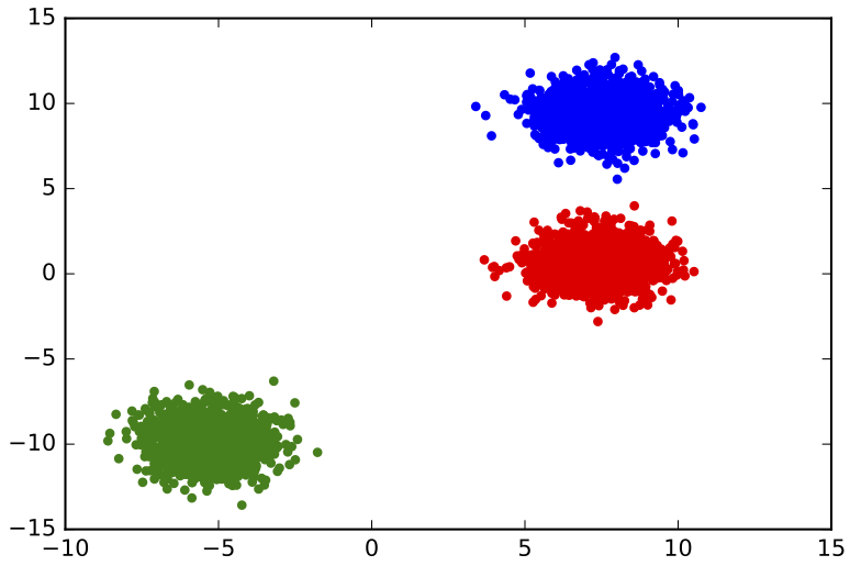
(a)  

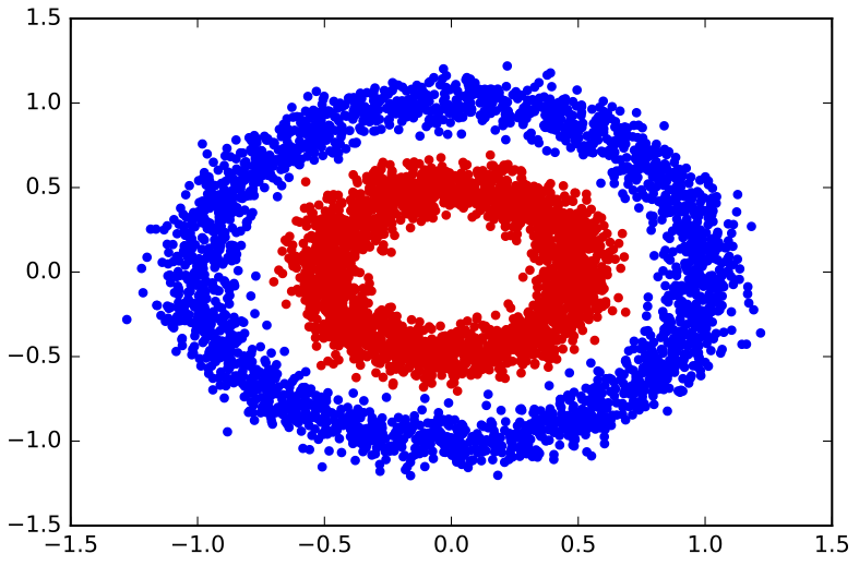
(b)  

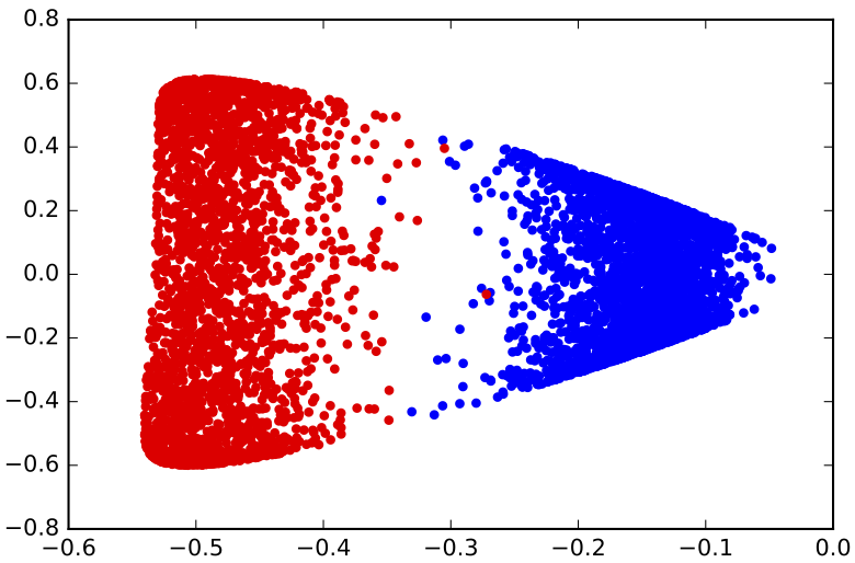
(c)  

Figure 1: Figures 1(a) and 1(b) show two sets of two-dimensional points, with different colors indicating different clusters. Figure 1(a) is separable using linear $k$-means; Figures 1(b) is inseparable using linear $k$-means. Figure 1(c) shows the first two dimensions of the feature vectors ${\bf k}_{1},\ldots,{\bf k}_{n}\in{\mathbb{R}}^{n}$ derived from a kernel.

To extend the scope of $k$-means clustering to include anistotropic, non-spherical clusters such as those depicted in Figure 1(b), Schölkopf et al. (1998) proposed to perform linear $k$-means clustering in a nonlinear feature space instead of the input space. After choosing a feature function $\mbox{\boldmath$\phi$\unboldmath}:{\mathbb{R}}^{d}\mapsto{\mathcal{F}}$ to map the input vectors non-linearly into feature vectors, they propose minimizing the objective function

$$\mathop{\rm argmin}_{{\mathcal{J}}_{1},\ldots,{\mathcal{J}}_{k}}\;\frac{1}{n}\sum_{i=1}^{k}\sum_{j\in{\mathcal{J}}_{i}}\bigg{\|}\mbox{\boldmath$\phi$\unboldmath}({\bf a}_{j})\>-\>\frac{1}{|{\mathcal{J}}_{i}|}\sum_{l\in{\mathcal{J}}_{i}}\mbox{\boldmath$\phi$\unboldmath}({\bf a}_{l})\bigg{\|}_{2}^{2},$$ (2)

where $\{{\mathcal{J}}_{1},\ldots,{\mathcal{J}}_{k}\}$ denotes a $k$-partition of $[n]$. The “kernel trick” enables us to minimize this objective without explicitly computing the potentially high-dimensional features, as inner products in feature space can be computed implicitly by evaluating the kernel function

$$\kappa\big{(}{\bf a}_{i},\,{\bf a}_{j}\big{)}\;=\;\big{\langle}\mbox{\boldmath$\phi$\unboldmath}({\bf a}_{i}),\,\mbox{\boldmath$\phi$\unboldmath}({\bf a}_{j})\big{\rangle}.$$

Thus the information required to solve the kernel $k$-means problem (2), is present in the kernel matrix ${\bf K}=[\kappa({\bf a}_{i},{\bf a}_{j})]_{ij}\in{\mathbb{R}}^{n\times n}$.

Let ${\bf K}={\bf V}\mbox{\boldmath$\Lambda$\unboldmath}{\bf V}^{T}$ be the full eigenvalue decomposition (EVD) of the kernel matrix and ${\bf k}_{1},\ldots,{\bf k}_{n}\in{\mathbb{R}}^{n}$ be the rows of ${\bf V}\mbox{\boldmath$\Lambda$\unboldmath}^{1/2}\in{\mathbb{R}}^{n\times n}$. It can be shown (see Appendix B.3) that the solution of (2) is identical to the solution of

$$\mathop{\rm argmin}_{{\mathcal{J}}_{1},\ldots,{\mathcal{J}}_{k}}\;\frac{1}{n}\sum_{i=1}^{k}\sum_{j\in{\mathcal{J}}_{i}}\bigg{\|}{\bf k}_{j}\>-\>\frac{1}{|{\mathcal{J}}_{i}|}\sum_{l\in{\mathcal{J}}_{i}}{\bf k}_{l}\bigg{\|}_{2}^{2}.$$ (3)

To demonstrate the power of kernel $k$-means clustering, consider the dataset in Figure 1(b). We use the Gaussian RBF kernel

$$\kappa({\bf a},{\bf a}^{\prime})=\exp\big{(}-\tfrac{1}{2\sigma^{2}}\|{\bf a}-{\bf a}^{\prime}\|_{2}^{2}\big{)}$$

with $\sigma=0.3$, and form the corresponding kernel matrix of the data in Figure 1(b). Figure 1(c) scatterplots the first two coordinates of the feature vectors ${\bf k}_{1},\ldots,{\bf k}_{n}$. Clearly, the first coordinate of the feature vectors already separates the two classes well, so $k$-means clustering using the non-linear features ${\bf k}_{1},\cdots,{\bf k}_{n}$ has a better chance of separating the two classes.

Although it is more generally applicable than linear $k$-means clustering, kernel $k$-means clustering is computationally expensive. As a baseline, we consider the cost of optimizing (3). The formation of the kernel matrix ${\bf K}$ given the input vectors ${\bf a}_{1},\ldots,{\bf a}_{n}\in{\mathbb{R}}^{d}$ costs ${\mathcal{O}}(n^{2}d)$ time. The objective in (3) can then be (approximately) minimized using Lloyd’s algorithm at a cost of ${\mathcal{O}}(n^{2}k)$ time per iteration. This requires the $n$-dimensional non-linear feature vectors obtained from the full EVD of ${\bf K}$; computing these feature vectors takes ${\mathcal{O}}(n^{3})$ time, because ${\bf K}$ is, in general, full-rank. Thus, approximately solving the kernel $k$-means clustering problem by optimizing (3) costs ${\mathcal{O}}(n^{3}+n^{2}d+Tn^{2}k)$ time, where $T$ is the number of iterations of Lloyd’s algorithm.

Kernel approximation techniques, including the Nyström method (Nyström, 1930; Williams and Seeger, 2001; Gittens and Mahoney, 2016) and random feature maps (Rahimi and Recht, 2007), have been applied to decrease the cost of solving kernelized machine learning problems: the idea is to replace ${\bf K}$ with a low-rank approximation, which allows for more efficient computations. Chitta et al. (2011, 2012) proposed to apply kernel approximations to efficiently approximate kernel $k$-means clustering. Although kernel approximations mitigate the computational challenges of kernel $k$-means clustering, the aforementioned works do not provide guarantees on the clustering performance: how accurate must the low-rank approximation of ${\bf K}$ be to ensure near optimality of the approximate clustering obtained via this method?

We propose a provable approximate solution to the kernel $k$-means problem based on the Nyström approximation. Our method has three steps: first, extract $c$ ($c\ll n$) features using the Nyström method; second, reduce the features to $s$ dimensions ($k\leq s<c$) using the truncated SVD; third, apply any off-the-shelf linear $k$-means clustering algorithm upon the $s$-dimensional features to obtain the final clusters. The total time complexity of the first two steps is ${\mathcal{O}}(ndc+nc^{2})$. The time complexity of the third step depends on the specific linear $k$-means algorithm; for example, using Lloyd’s algorithm, the per-iteration complexity is ${\mathcal{O}}(nsk)$, and the number of iterations may depend on $s$.

Our method comes with a strong approximation ratio guarantee. Suppose we set $s={k}/{\epsilon}$ and $c=\tilde{{\mathcal{O}}}(\mu s/\epsilon)$ for any $\epsilon\in(0,1)$, where $\mu\in[1,\tfrac{n}{s}]$ is the coherence parameter of the dominant $s$-dimensional singular space of the kernel matrix ${\bf K}$. Also suppose the standard kernel $k$-means and our approximate method use the same linear $k$-means clustering algorithm, e.g., Lloyd’s algorithm or some other algorithm that comes with different provable approximation guarantees. As guaranteed by Theorem 2, when the quality of the clustering is measured by the cost function defined in (2), with probability at least $0.9$, our algorithm returns a clustering that is at most $1+{\mathcal{O}}(\epsilon)$ times worse than the standard kernel $k$-means clustering. Our theory makes explicit the trade-off between accuracy and computation: larger $s$ and $c$ lead to high accuracy and also high computational cost.

Spectral clustering (Shi and Malik, 2000; Ng et al., 2002) is a popular alternative to kernel $k$-means clustering that can also partition non-linearly separable data such as those in Figure 1(b). Unfortunately, because it requires computing an $n\times n$ affinity matrix and the top $k$ eigenvectors of the corresponding graph Laplacian, spectral clustering is inefficient for large $n$. Fowlkes et al. (2004) applied the Nyström approximation to increase the scalability of spectral clustering. Since then, spectral clustering with Nyström approximation has been used in many works, e.g., (Arikan, 2006; Berg et al., 2004; Chen et al., 2011; Wang et al., 2016b; Weiss et al., 2009; Zhang and Kwok, 2010). Despite its popularity in practice, this approach does not come with guarantees on the approximation ratio for the obtained clustering. Our algorithm, which combines kernel $k$-means with Nyström approximation, is an equally computationally efficient alternative that comes with strong bounds on the approximation ratio, and can be used wherever spectral clustering is applied.

1.1 Contributions

Using tools developed in (Boutsidis et al., 2015; Cohen et al., 2015; Feldman et al., 2013), we rigorously analyze the performance of approximate kernel $k$-means clustering with the Nyström approximation, and show that a rank-$\tfrac{k}{\epsilon}$ Nyström approximation delivers a $1+{\mathcal{O}}(\epsilon)$ approximation ratio guarantee, relative to the guarantee provided by the same algorithm without the use of the Nyström method.

As part of the analysis of kernel $k$-means with Nyström approximation, we establish the first relative-error bound for rank-restricted Nyström approximation, which has independent interest.

Kernel $k$-means clustering and spectral clustering are competing solutions to the nonlinear clustering problem, neither of which scales well with $n$. Fowlkes et al. (2004) introduced the use of Nyström approximations to make spectral clustering scalable; this approach has become popular in machine learning. We identify fundamental mathematical problems with this heuristic. These concerns and an empirical comparison establish that our proposed combination of kernel $k$-means with rank-restricted Nyström approximation is a theoretically well-founded and empirically competitive alternative to spectral clustering with Nyström approximation.

Finally, we demonstrate the scalability of this approach by measuring the performance of an Apache Spark implementation of a distributed version of our approximate kernel $k$-means clustering algorithm using the MNIST8M data set, which has $8.1$ million instances and $10$ classes.

1.2 Relation to Prior Work

The key to our analysis of the proposed approximate kernel $k$-means clustering algorithm is a novel relative-error trace norm bound for a rank-restricted Nyström approximation. We restrict the rank of the Nyström approximation in a non-standard manner (see Remark 1). Our relative-error trace norm bound is not a simple consequence of the existing bounds for non-rank-restricted Nyström approximation such as the ones provided by Gittens and Mahoney (2016). The relative-error bound which we provide for the rank-restricted Nyström approximation is potentially useful in other applications involving the Nyström method.

The projection-cost preservation (PCP) property (Cohen et al., 2015; Feldman et al., 2013) is an important tool for analyzing approximate linear $k$-means clustering. We apply our novel relative-error trace norm bound as well as existing tools in (Cohen et al., 2015) to prove that the rank-restricted Nyström approximation enjoys the PCP property. We do not rule out the possibility that the non-rank-restricted (rank-$c$) Nyström approximation satisfies the PCP property and/or also enjoys a $1+\epsilon$ approximation ratio guarantee when applied to kernel $k$-means clustering. However, the cost of the linear $k$-means clustering step in the algorithm is proportional to the dimensionality of the feature vectors, so the rank-restricted Nyström approximation, which produces $s$-dimensional feature vectors, where $s<c$, is more computationally desirable.

Musco and Musco (2017) similarly establishes a $1+\epsilon$ approximation ratio for the kernel $k$-means objective when a Nyström approximation is used in place of the full kernel matrix. Specifically, Musco and Musco (2017) shows that when $c={\mathcal{O}}(\tfrac{k}{\epsilon}\log\tfrac{k}{\epsilon})$ columns of ${\bf K}$ are sampled using ridge leverage score (RLS) sampling (Alaoui and Mahoney, 2015; Cohen et al., 2017; Musco and Musco, 2017) and are used to form a Nyström approximation, then applying linear $k$-means clustering to the $c$-dimensional Nyström features returns a clustering that has objective value at most $1+\epsilon$ times as large as the objective value of the best clustering. Our theory is independent of that in Musco and Musco (2017), and differs in that (1) Musco and Musco (2017) applies specifically to Nyström approximations formed using RLS sampling, whereas our guarantees apply to any sketching method that satisfies the “subspace embedding” and “matrix multiplication” properties (see Lemma 10 for definitions of these two properties); (2) Musco and Musco (2017) establishes a $1+\epsilon$ approximation ratio for the non-rank-restricted RLS-Nyström approximation, whereas we establish a $1+\epsilon$ approximation ratio for the (more computationally efficient) rank-restricted Nyström approximation.

1.3 Paper Organization

In Section 2, we start with a definition of the notation used throughout this paper as well as a background on matrix sketching methods. Then, in Section 3, we present our main theoretical results: Section 3.1 presents an improved relative-error rank-restricted Nyström approximation; Section 3.2 presents the main theoretical results on kernel $k$-means with Nyström approximation; and Section 3.3 studies kernel $k$-means with kernel principal component analysis. Section 4 discusses and evaluates the theoretical and empirical merits of kernel $k$-means clustering versus spectral clustering, when each is approximated using Nyström approximation. Section 5 empirically compares the Nyström method and the random feature maps for the kernel $k$-means clustering on medium-scale data. Section 6 presents a large-scale distributed implementation in Apache Spark and its empirical evaluation on a data set with $8.1$ million points. Section 7 provides a brief conclusion. Proofs are provided in the Appendices.

2 Notation

This section defines the notation used throughout this paper. A set of commonly used parameters is summarized in Table 1.

Table 1: Commonly used parameters. It holds that $k\leq s\leq c\leq n$.

Notation	Definition
$n$	number of samples
$d$	number of features (attributes)
$k$	number of clusters
$s$	target rank of the Nyström approximation
$c$	sketch size of the Nyström approximation

Matrices and vectors.

We take ${\bf I}_{n}$ to be the $n\times n$ identity matrix, ${\bf 0}$ to be a vector or matrix of all zeros of the appropriate size, and ${\bf 1}_{n}$ to be the $n$-dimensional vector of all ones.

Sets.

The set $\{1,2,\cdots,n\}$ is written as $[n]$. We call $\{{\mathcal{J}}_{1},\cdots,{\mathcal{J}}_{k}\}$ a $k$-partition of $[n]$ if ${\mathcal{J}}_{1}\cup\cdots\cup{\mathcal{J}}_{k}=[n]$ and ${\mathcal{J}}_{p}\cap{\mathcal{J}}_{q}=\emptyset$ when $p\neq q$. Let $|{\mathcal{J}}|$ denote the cardinality of the set ${\mathcal{J}}$.

Singular value decomposition (SVD).

Let ${\bf A}\in{\mathbb{R}}^{n\times d}$ and $\rho=\mathrm{rank}({\bf A})$. A (compact) singular value decomposition (SVD) is defined by

$$\textstyle{{\bf A}\;=\;{\bf U}\mbox{\boldmath$\Sigma$\unboldmath}{\bf V}^{T}\;=\;\sum_{i=1}^{\rho}\sigma_{i}({\bf A}){\bf u}_{i}{\bf v}_{i}^{T},}$$

where ${\bf U}$, $\Sigma$, ${\bf V}$ are an $n\times\rho$ column-orthogonal matrix, a $\rho\times\rho$ diagonal matrix with nonnegative entries, and a $d\times\rho$ column-orthogonal matrix, respectively. If ${\bf A}$ is symmetric positive semi-definite (SPSD), then ${\bf U}={\bf V}$, and this decomposition is also called the (reduced) eigenvalue decomposition (EVD). By convention, we take $\sigma_{1}({\bf A})\geq\cdots\geq\sigma_{\rho}({\bf A})$.

Truncated SVD.

The matrix ${\bf A}_{s}=\sum_{i=1}^{s}\sigma_{i}({\bf A}){\bf u}_{i}{\bf v}_{i}^{T}$ is a rank-$s$ truncated SVD of ${\bf A}$, and is an optimal rank-$s$ approximation to ${\bf A}$ when the approximation error is measured in a unitarily invariant norm.

The Moore-Penrose inverse

of ${\bf A}$ is defined by ${\bf A}^{\dagger}={\bf V}\mbox{\boldmath$\Sigma$\unboldmath}^{-1}{\bf U}^{T}$.

Leverage score and coherence.

Let ${\bf U}\in{\mathbb{R}}^{n\times\rho}$ be defined in the above and ${\bf u}_{i}$ be the $i$-th row of ${\bf U}$. The row leverage scores of ${\bf A}$ are $l_{i}=\|{\bf u}_{i}\|_{2}^{2}$ for $i\in[n]$. The row coherence of ${\bf A}$ is $\mu({\bf A})=\frac{n}{\rho}\max_{i}\|{\bf u}_{i}\|_{2}^{2}$. The leverage scores for a matrix ${\bf A}$ can be computed exactly in the time it takes to compute the matrix ${\bf U}$; and the leverage scores can be approximated (in theory (Drineas et al., 2012) and in practice (Gittens and Mahoney, 2016)) in roughly the time it takes to apply a random projection matrix to the matrix ${\bf A}$.

Matrix norms.

We use three matrix norms in this paper:

Frobenius Norm: $$\|{\bf A}\|_{F}\;=\;\sqrt{{\textstyle\sum_{i,j}}a_{ij}^{2}}\;=\;\sqrt{{\textstyle\sum_{i}}\sigma_{i}^{2}({\bf A})};$$

Spectral Norm: $$\|{\bf A}\|_{2}\;=\;\max_{\|{\bf x}\|_{2}=1}\big{\|}{\bf A}{\bf x}\big{\|}_{2}\;=\;\sigma_{1}({\bf A});$$

Trace Norm: $$\|{\bf A}\|_{*}\;=\;{\textstyle\sum_{i}}\sigma_{i}({\bf A}).$$

Any square matrix satisfies $\mathrm{tr}({\bf A})\leq\|{\bf A}\|_{*}$. If additionally ${\bf A}$ is SPSD, then $\mathrm{tr}({\bf A})=\|{\bf A}\|_{*}$.

Matrix sketching

Here, we briefly review matrix sketching methods that are commonly used within randomized linear algebra (RLA) (Mahoney, 2011).

Given a matrix ${\bf A}\in{\mathbb{R}}^{m\times n}$, we call ${\bf C}={\bf A}{\bf P}\in{\mathbb{R}}^{m\times c}$ (typically $c\ll n$) a sketch of ${\bf A}$ and ${\bf P}\in{\mathbb{R}}^{n\times c}$ a sketching matrix. Within RLA, sketching has emerged as a powerful primitive, where one is primarily interested in using random projections and random sampling to construct randomzed sketches (Mahoney, 2011; Drineas and Mahoney, 2016). In particular, sketching is useful as it allows large matrices to be replaced with smaller matrices which are more amenable to efficient computation, but provably retain almost optimal accuracy in many computations (Mahoney, 2011; Woodruff, 2014). The columns of ${\bf C}$ typically comprise a rescaled subset of the columns of ${\bf A}$, or random linear combinations of the columns of ${\bf A}$; the former type of sketching is called column selection or random sampling, and the latter is referred to as random projection.

Column selection forms ${\bf C}\in{\mathbb{R}}^{m\times c}$ using a randomly sampled and rescaled subset of the columns of ${\bf A}\in{\mathbb{R}}^{m\times n}$. Let $p_{1},\cdots,p_{n}\in(0,1)$ be the sampling probabilities associated with the columns of ${\bf A}$ (so that, in particular, $\sum_{i=1}^{n}p_{i}=1$). The columns of the sketch are selected identically and independently as follows: each column of ${\bf C}$ is randomly sampled from the columns of ${\bf A}$ according to the sampling probabilities and rescaled by $\frac{1}{\sqrt{cp_{i}}},$ where $i$ is the index of the column of ${\bf A}$ that was selected. In our matrix multiplication formulation for sketching, column selection corresponds to a sketching matrix ${\bf P}\in{\mathbb{R}}^{n\times c}$ that has exactly one non-zero entry in each column, whose position and magnitude correspond to the index of the column selected from ${\bf A}$. Uniform sampling is column sampling with $p_{1}=\cdots=p_{n}=\frac{1}{n}$, and leverage score sampling takes $p_{i}=\tfrac{l_{i}}{\sum_{j}l_{j}}$ for $i\in[n]$, where $l_{i}$ is the $i$-th leverage score of some matrix (typically ${\bf A}$, ${\bf A}_{k}$, or an randomized approximation thereto) (Drineas et al., 2012).

Gaussian projection is a type of random projection where the sketching matrix is taken to be ${\bf P}=\frac{1}{\sqrt{c}}{\bf G}\in{\mathbb{R}}^{n\times c}$; here the entries of ${\bf G}$ are i.i.d. ${\mathcal{N}}(0,1)$ random variables. Gaussian projection is inefficient relative to column sampling: the formation of a Gaussian sketch of a dense $m\times n$ matrix requires ${\mathcal{O}}(mnc)$ time. The Subsampled Randomized Hadamard Transform (SRHT) is a more efficient alternative that enjoys similar properties to the Gaussian projection (Drineas et al., 2011; Lu et al., 2013; Tropp, 2011), and can be applied to a dense $m\times n$ matrix in only ${\mathcal{O}}(mn\log c)$ time. The CountSketch is even more efficient: it can be applied to any matrix ${\bf A}$ in ${\mathcal{O}}(\mathrm{nnz}({\bf A}))$ time (Clarkson and Woodruff, 2013; Meng and Mahoney, 2013; Nelson and Nguyên, 2013), where $\mathrm{nnz}(\cdot)$ denotes the number of nonzero entries in a matrix.

3 Our Main Results: Improved SPSD Matrix Approximation and Kernel $k$-means Approximation

In this section, we present our main theoretical results. We start, in Section 3.1, by presenting Theorem 1, a novel result on SPSD matrix approximation with the rank-restricted Nyström method. This result is of independent interest, and so we present it in detail, but in this paper we will use it to establish our main result. Then, in Section 3.2, we present Theorem 2, which is our main result for approximate kernel $k$-means with the Nyström approximation. In Section 3.3, we establish novel guarantees on kernel $k$-means with dimensionality reduction.

3.1 The Nyström Method

The Nyström method (Nyström, 1930) is the most popular kernel approximation method in the machine learning community. Let ${\bf K}\in{\mathbb{R}}^{n\times n}$ be an SPSD matrix and ${\bf P}\in{\mathbb{R}}^{n\times c}$ be a sketching matrix. The Nyström method approximates ${\bf K}$ with ${\bf C}{\bf W}^{\dagger}{\bf C}^{T}$, where ${\bf C}={\bf K}{\bf P}$ and ${\bf W}={\bf P}^{T}{\bf K}{\bf P}$. The Nyström method was introduced to the machine learning community by Williams and Seeger (2001); since then, numerous works have studied its theoretical properties, e.g., (Drineas and Mahoney, 2005; Gittens and Mahoney, 2016; Jin et al., 2013; Kumar et al., 2012; Wang and Zhang, 2013; Yang et al., 2012).

Empirical results in (Gittens and Mahoney, 2016; Wang et al., 2016b; Yang et al., 2012) demonstrated that the accuracy of the Nyström method significantly increases when the spectrum of ${\bf K}$ decays fast. This suggests that the Nyström approximation captures the dominant eigenspaces of ${\bf K}$, and that error bounds comparing the accuracy of the Nyström approximation of ${\bf K}$ to that of the best rank-$s$ approximation ${\bf K}_{s}$ (for $s<c$) would provide a meaningful measure of the performance of the Nyström kernel approximation. Gittens and Mahoney (2016) established the first relative-error bounds showing that for sufficiently large $c$, the trace norm error $\|{\bf K}-{\bf C}{\bf W}^{\dagger}{\bf C}^{T}\|_{*}$ is comparable to $\|{\bf K}-{\bf K}_{s}\|_{*}$. Such results quantify the benefits of spectral decay to the performance of the Nyström method, and are sufficient to analyze the performance of Nyström approximations in applications such as kernel ridge regression (Alaoui and Mahoney, 2015; Bach, 2013) and kernel support vector machines (Cortes et al., 2010).

However, Gittens and Mahoney (2016) did not analyze the performance of rank-restricted Nyström approximations; they compared the approximation accuracies of the rank-$c$ matrix ${\bf C}{\bf W}^{\dagger}{\bf C}^{T}$ and the rank-$s$ matrix ${\bf K}_{s}$ (recall $s<c$). In our application to approximate kernel $k$-means clustering, it is the rank-$s$ matrix $({\bf C}{\bf W}^{\dagger}{\bf C}^{T})_{s}$ that is of relevance. Given ${\bf C}$ and ${\bf W}$, the truncated SVD $\big{(}({\bf W}^{\dagger})^{1/2}{\bf C}^{T}\big{)}_{s}=\tilde{{\bf U}}_{s}\tilde{\mbox{\boldmath$\Sigma$\unboldmath}}_{s}\tilde{{\bf V}}_{s}^{T}$ can be found using ${\mathcal{O}}(nc^{2})$ time. Then the rank-$s$ Nyström approximation can be written as

$$({\bf C}{\bf W}^{\dagger}{\bf C}^{T})_{s}\;=\;\big{(}{\bf C}({\bf W}^{\dagger})^{1/2}\big{)}_{s}\big{(}{\bf C}({\bf W}^{\dagger})^{1/2}\big{)}_{s}^{T}\;=\;\tilde{{\bf V}}_{s}\tilde{\mbox{\boldmath$\Sigma$\unboldmath}}_{s}^{2}\tilde{{\bf V}}_{s}^{T}.$$ (4)

Theorem 1 provides a relative-error trace norm approximation guarantee for the sketch (4) and is novel; a proof is provided in Appendix A.

Theorem 1 (Relative-Error Rank-Restricted Nyström Approximation)

Let ${\bf K}\in{\mathbb{R}}^{n\times n}$ be an SPSD matrix, $s$ be the target rank, and $\epsilon\in(0,1)$ be an error parameter. Let ${\bf P}\in{\mathbb{R}}^{n\times c}$ be a sketching matrix corresponding to one of the sketching methods listed in Table 2. Let ${\bf C}={\bf K}{\bf P}$ and ${\bf W}={\bf P}^{T}{\bf K}{\bf P}$. Then

$$\big{\|}{\bf K}-({\bf C}{\bf W}^{\dagger}{\bf C}^{T})_{s}\big{\|}_{*} \leq (1+\epsilon)\,\big{\|}{\bf K}-{\bf K}_{s}\big{\|}_{*}$$

holds with probability at least $0.9$. In addition, there exists an $n\times s$ column orthogonal matrix ${\bf Q}$ such that $({\bf C}{\bf W}^{\dagger}{\bf C}^{T})_{s}={\bf K}^{1/2}{\bf Q}{\bf Q}^{T}{\bf K}^{1/2}$.

Table 2: Sufficient sketch sizes for several sketching methods used to construct Nyström approximations to the matrix ${\bf K}$. Let ${\bf K}_{s}={\bf V}_{s}\mbox{\boldmath$\Sigma$\unboldmath}_{s}{\bf V}_{s}^{T}$ be the truncated SVD of ${\bf K}$, then $\mu$ denotes the row coherence of ${\bf V}_{s}\in{\mathbb{R}}^{n\times s}$ and the leverage score sampling is done using the row leverage scores of ${\bf V}_{s}$.

sketching	sketch size ($c$)	time complexity ($T$)
uniform sampling	${\mathcal{O}}(\mu{s}/{\epsilon}+\mu s\log s)$	${\mathcal{O}}(nc)$
leverage sampling	${\mathcal{O}}({s}/{\epsilon}+s\log s)$	$\tilde{\mathcal{O}}(n^{2}s)$
Gaussian projection	${\mathcal{O}}({s}/{\epsilon})$	${\mathcal{O}}(n^{2}c)$
SRHT	${\mathcal{O}}((s+\log n)(\epsilon^{-1}+\log s))$	${\mathcal{O}}(n^{2}\log c)$
CountSketch	${\mathcal{O}}(s/\epsilon+s^{2})$	${\mathcal{O}}(n^{2})$

Remark 1 (Rank Restrictions)

The traditional rank-restricted Nyström approximation, ${\bf C}({\bf W}_{s})^{\dagger}{\bf C}^{T}$, (Drineas and Mahoney, 2005; Fowlkes et al., 2004; Gittens and Mahoney, 2016; Li et al., 2015) is not known to satisfy a relative-error bound of the form guaranteed in Theorem 1. Pourkamali-Anaraki and Becker (2016) pointed out the drawbacks of the traditional rank-restricted Nyström approximation and proposed the use of the rank-restricted Nyström approximation $({\bf C}{\bf W}^{\dagger}{\bf C}^{T})_{s}$ in applications requiring kernel approximations, but provided only empirical evidence of its performance. This work provides guarantees on the approximation error of the rank-restricted Nyström approximation $({\bf C}{\bf W}^{\dagger}{\bf C}^{T})_{s}$, and applies this approximation to the kernel $k$-means clustering problem. The contemporaneous work Tropp et al. (2017) provides similar guarantees on the approximation error of $({\bf C}{\bf W}^{\dagger}{\bf C}^{T})_{s}$, and uses this Nyström approximation as the basis of a streaming algorithm for fixed-rank approximation of positive-semidefinite matrices.

3.2 Main Result for Approximate Kernel $k$-means

In this section we establish the approximation ratio guarantees for the objective function of kernel $k$-means clustering. We first define $\gamma$-approximate $k$-means algorithms (where $\gamma\geq 1$), then present our main result in Theorem 2.

Let ${\bf A}$ be a matrix with $n$ rows ${\bf a}_{1},\cdots,{\bf a}_{n}$. The objective function for linear $k$-means clustering over the rows of ${\bf A}$ is

$$f\big{(}{\mathcal{J}}_{1},\cdots,{\mathcal{J}}_{k}\,;\,{\bf A}\big{)}\;=\;\frac{1}{n}\sum_{i=1}^{k}\sum_{j\in{\mathcal{J}}_{i}}\bigg{\|}{\bf a}_{j}\>-\>\frac{1}{|{\mathcal{J}}_{i}|}\sum_{l\in{\mathcal{J}}_{i}}{\bf a}_{l}\bigg{\|}_{2}^{2}.$$

The minimization of $f$ w.r.t. the $k$-partition $\{{\mathcal{J}}_{1},\cdots,{\mathcal{J}}_{k}\}$ is NP-hard (Garey et al., 1982; Aloise et al., 2009; Dasgupta and Freund, 2009; Mahajan et al., 2009; Awasthi et al., 2015), but approximate solutions can be obtained in polynomial time. $\gamma$-approximate algorithms capture one useful notion of approximation.

Definition 1 ($\gamma$-Approximate Algorithms)

A linear $k$-means clustering algorithm ${\mathcal{A}}_{\gamma}$ takes as input a matrix ${\bf Z}$ with $n$ rows and outputs $\{{{\mathcal{J}}}_{1}^{\prime},\cdots,{{\mathcal{J}}}_{k}^{\prime}\}$. We call ${\mathcal{A}}_{\gamma}$ a $\gamma$-approximate algorithm if, for any such matrix ${\bf Z}$,

$$f\big{(}{\mathcal{J}}_{1}^{\prime},\cdots,{\mathcal{J}}_{k}^{\prime}\,;\,{\bf Z}\big{)} \leq \gamma\,\cdot\,\min_{{\mathcal{J}}_{1},\cdots,{\mathcal{J}}_{k}}\;f\big{(}{\mathcal{J}}_{1},\cdots,{\mathcal{J}}_{k}\,;\,{\bf Z}\big{)}.$$

Here $\{{{\mathcal{J}}}_{1},\cdots,{{\mathcal{J}}}_{k}\}$ and $\{{{\mathcal{J}}}_{1}^{\prime},\cdots,{{\mathcal{J}}}_{k}^{\prime}\}$ are $k$-partitions of $[n]$.

Many $(1+\epsilon)$-approximation algorithms have been proposed, but they are computationally expensive (Chen, 2009; Har-Peled and Mazumdar, 2004; Kumar et al., 2004; Matousek, 2000). There are also relatively efficient constant factor approximate algorithms, e.g., (Arthur and Vassilvitskii, 2007; Kanungo et al., 2002; Song and Rajasekaran, 2010).

Let $\phi$ be a feature map, $\Phi$ be the matrix with rows $\phi({\bf a}_{1}),\ldots,\phi({\bf a}_{n})$, and ${\bf K}=\mbox{\boldmath$\Phi$\unboldmath}\mbox{\boldmath$\Phi$\unboldmath}^{T}\in{\bf R}^{n\times n}$ be the associated kernel matrix. Analogously, we denote the objective function for kernel $k$-means clustering by

$$f\big{(}{\mathcal{J}}_{1},\cdots,{\mathcal{J}}_{k}\;;\;\mbox{\boldmath$\Phi$\unboldmath}\big{)}\;=\;\frac{1}{n}\sum_{i=1}^{k}\sum_{j\in{\mathcal{J}}_{i}}\bigg{\|}\mbox{\boldmath$\phi$\unboldmath}({\bf a}_{j})\>-\>\frac{1}{|{\mathcal{J}}_{i}|}\sum_{l\in{\mathcal{J}}_{i}}\mbox{\boldmath$\phi$\unboldmath}({\bf a}_{l})\bigg{\|}_{2}^{2},$$

where $\{{\mathcal{J}}_{1},\cdots,{\mathcal{J}}_{k}\}$ is a $k$-partition of $[n]$.

Theorem 2 (Kernel $k$-Means with Nyström Approximation)

Choose a sketching matrix ${\bf P}\in{\mathbb{R}}^{n\times c}$ and sketch size $c$ consistent with Table 2. Let ${\bf C}{\bf W}^{\dagger}{\bf C}^{T}$ be the previously defined Nyström approximation of ${\bf K}$. Let ${\bf B}\in{\mathbb{R}}^{n\times s}$ be any matrix satisfying ${\bf B}{\bf B}^{T}=({\bf C}{\bf W}^{\dagger}{\bf C}^{T})_{s}$. Let the $k$-partition $\{\tilde{{\mathcal{J}}}_{1},\cdots,\tilde{{\mathcal{J}}}_{k}\}$ be the output of a $\gamma$-approximate algorithm applied to the rows of ${\bf B}$. With probability at least $0.9$,

$$f\big{(}\tilde{{\mathcal{J}}}_{1},\cdots,\tilde{{\mathcal{J}}}_{k}\;;\;\mbox{\boldmath$\Phi$\unboldmath}\big{)} \leq \gamma\big{(}1+\epsilon+\tfrac{k}{s}\big{)}\,\cdot\,\min_{{\mathcal{J}}_{1},\cdots,{\mathcal{J}}_{k}}\;f\big{(}{\mathcal{J}}_{1},\cdots,{\mathcal{J}}_{k}\;;\;\mbox{\boldmath$\Phi$\unboldmath}\big{)}.$$

Remark 2

Kernel $k$-means clustering is an NP-hard problem. Therefore, instead of comparing with $\min f$, we compare with clusterings obtained using $\gamma$-approximate algorithms. Theorem 2 shows that, when uniform sampling to form the Nyström approximation, if $s={\mathcal{O}}(\frac{k}{\epsilon})$ and $c=\tilde{{\mathcal{O}}}(\frac{\mu s}{\epsilon})$, then the returned clustering has an objective value that is at most a factor of $\epsilon$ larger than the objective value of the kernel $k$-means clustering returned by the $\gamma$-approximate algorithm.

Remark 3

Assume we are in a practical setting where $c$, the budget of column samples one can use to form a Nyström approximation, and $k$, the number of desired cluster centers, are fixed. The pertinent question is how to choose $s$ to produce a high-quality approximate clustering. Theorem 2 shows that for uniform sampling, the error ratio is

$$1+\epsilon+\tfrac{k}{s}\;=\;1+\tilde{{\mathcal{O}}}(\tfrac{s\mu}{c})+\tfrac{k}{s}.$$

To balance the two sources of error, $s$ must be larger than $k$, but not too large a fraction of $c$. To minimize the above error ratio, $s$ should be selected on the order of $\sqrt{{kc}/{\mu}}$. Since the matrix coherence $\mu$ ($\geq 1$) is unknown, it can be heuristically treated as a constant.

We empirically study the effect of the values of $c$ and $s$ using a data set comprising $8.1$ million samples. Note that computing the kernel $k$-means clustering objective function requires the formation of the entire kernel matrix ${\bf K}$, which is infeasible for a data set of this size; instead, we use normalized mutual information (NMI) (Strehl and Ghosh, 2002)—a standard measure of the performance of clustering algorithms— to measure the quality of the clustering obtained by approximating kernel $k$-means clustering using Nyström approximations formed through uniform sampling. NMI scores range from zero to one, with a larger score indicating better performance. We report the results in Figure 2. The complete details of the experiments, including the experimental setting and time costs, are given in Section 6.

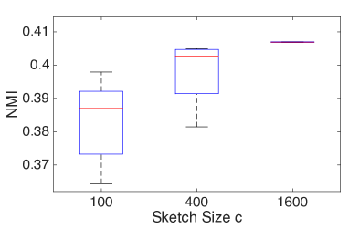
(a) Fix $s=20$ and vary $c$.

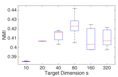
(b) Fix $c=1600$ and vary $s$.

Figure 2: Performance of approximate kernel $k$-means clustering on the MNIST8M data set, for which $n=8.1\times 10^{6}$, $d=784$, and $k=10$. We use Nyström approximations formed using uniform sampling, and the built-in $k$-means algorithm of Spark MLlib (a parallelized variant of the $k$-means++ method) with the setting $\textsf{MaxIter}=100$.

From Figure 2(a) we observe that larger values of $c$ lead to better and more stable clusterings: the mean of the NMI increases and its standard deviation decreases. This is reasonable and in accordance with our theory. However, larger values of $c$ incur more computations, so one should choose $c$ to trade off computation and accuracy.

Figure 2(b) shows that for fixed $k$ and $c$, the clustering performance is not monotonic in $s$, which matches Theorem 2 (see the discussion in Remark 3). Setting $s$ as small as $k$ results in poor performance. Setting $s$ over-large not only incurs more computations, but also negatively affects clustering performance; this may suggest the necessity of rank-restriction. Furthermore, in this example, $\sqrt{kc}=126.5$, which corroborates the suggestion made in Remark 3 that setting $s$ around $\sqrt{kc/\mu}$ (where $\mu$ is unknown but can be treated as a constant larger than $1$) can be a good choice.

Remark 4

Musco and Musco (2017) established a $1+\epsilon$ approximation ratio for the kernel $k$-means objective value when a non-rank-restricted Nyström approximation is formed using ridge leverage scores (RLS) sampling; their analysis is specific to RLS sampling and does not extend to other sketching methods. By way of comparison, our analysis covers several popular sampling schemes and applies to rank-restricted Nyström approximations, but does not extend to RLS sampling.

3.3 Approximate Kernel $k$-Means with KPCA and Power Method

The use of dimensionality reduction to increase the computational efficiency of $k$-means clustering has been widely studied, e.g. in (Boutsidis et al., 2010, 2015; Cohen et al., 2015; Feldman et al., 2013; Zha et al., 2002). Kernel principal component analysis (KPCA) is particularly well-suited to this application (Dhillon et al., 2004; Ding et al., 2005). Applying Lloyd’s algorithm on the rows of $\Phi$ or ${\bf K}^{-1/2}$ has an ${\mathcal{O}}(n^{2}k)$ per-iteration complexity; if $s$ features are extracted using KPCA and Lloyd’s algorithm is applied to the resulting $s$-dimensional feature map, then the per-iteration cost reduces to ${\mathcal{O}}(nsk).$ Proposition 3 states that, to obtain a $1+\epsilon$ approximation ratio in terms of the kernel $k$-means objective function, it suffices to use $s=\frac{k}{\epsilon}$ KPCA features. This proposition is a simple consequence of (Cohen et al., 2015).

Proposition 3 (KPCA)

Let $\Phi$ be a matrix with $n$ rows, and ${\bf K}=\mbox{\boldmath$\Phi$\unboldmath}\mbox{\boldmath$\Phi$\unboldmath}^{T}\in{\bf R}^{n\times n}$ be the corresponding kernel matrix. Let ${\bf K}_{s}={\bf V}_{s}\mbox{\boldmath$\Lambda$\unboldmath}_{s}{\bf V}_{s}^{T}$ be the truncated SVD of ${\bf K}$ and take ${\bf B}={\bf V}_{s}\mbox{\boldmath$\Lambda$\unboldmath}_{s}^{1/2}\in{\mathbb{R}}^{n\times s}$. Let the $k$-partition $\{\tilde{{\mathcal{J}}}_{1},\cdots,\tilde{{\mathcal{J}}}_{k}\}$ be the output of a $\gamma$-approximate algorithm applied to the rows of ${\bf B}$. Then

$$f\big{(}\tilde{{\mathcal{J}}}_{1},\cdots,\tilde{{\mathcal{J}}}_{k}\;;\;\mbox{\boldmath$\Phi$\unboldmath}\big{)} \leq \gamma\,\big{(}1+\tfrac{k}{s}\big{)}\,\cdot\,\min_{{\mathcal{J}}_{1},\cdots,{\mathcal{J}}_{k}}\;f\big{(}{\mathcal{J}}_{1},\cdots,{\mathcal{J}}_{k}\;;\;\mbox{\boldmath$\Phi$\unboldmath}\big{)}.$$

In practice, the truncated SVD (equivalently EVD) of ${\bf K}$ is computed using the power method or Krylov subspace methods. These numerical methods do not compute the exact decomposition ${\bf K}_{s}={\bf V}_{s}\mbox{\boldmath$\Lambda$\unboldmath}_{s}{\bf V}_{s}^{T}$, so Proposition 3 is not directly applicable. It is useful to have a theory that captures the effect of realisticly inaccurate estimates like ${\bf K}_{s}\approx\tilde{{\bf V}}_{s}\tilde{\mbox{\boldmath$\Lambda$\unboldmath}}_{s}\tilde{{\bf V}}_{s}^{T}$ on the clustering process. As one particular example, consider that general-purpose implementations of the truncated SVD attempt to mitigate the fact that the computed decompositions are inaccurate by returning very high-precision solutions, e.g. solutions that satisfy $\|({\bf I}_{n}-{\bf V}_{s}{\bf V}_{s}^{T})\tilde{{\bf V}}_{s}\|_{2}\leq 10^{-10}$. Understanding the trade-off between the precision of the truncated SVD solution and the impact on the approximation ratio of the approximate kernel $k$-means solution allows us to more precisely manage the computational complexity of our algorithms. Are such high-precision solutions necessary for kernel $k$-means clustering?

Theorem 4 answers this question by establishing that highly accurate eigenspaces are not significantly more useful in approximate kernel $k$-means clustering than eigenspace estimates with lower accuracy. A low-precision solution obtained by running the power iteration for a few rounds suffices for kernel $k$-means clustering applications. We prove Theorem 4 in Appendix C.

Algorithm 1 Approximate Kernel $k$-Means using the Power Method.

1:  Input: kernel matrix ${\bf K}\in{\mathbb{R}}^{n\times n}$, number of clusters $k$, target dimension $s$ ($\geq k$), sketch size $c$ ($\geq s$), number of iterations $t$ ($\geq 1$)

2:  Draw a Gaussian projection matrix ${\bf P}\in{\mathbb{R}}^{n\times c}$;

3:  for all $j\in[t]$ do

4:     ${\bf P}\longleftarrow{\bf K}{\bf P}$;

5:  end for

6:  Orthogonalize ${\bf P}$ to obtain ${\bf U}\in{\mathbb{R}}^{n\times c}$;

7:  Compute ${\bf C}={\bf K}{\bf U}$ and ${\bf W}={\bf U}^{T}{\bf K}{\bf U}$;

8:  Compute a ${\bf B}\in{\mathbb{R}}^{n\times s}$ satisfying $({\bf C}{\bf W}^{\dagger}{\bf C}^{T})_{s}={\bf B}{\bf B}^{T}$;

9:  return  ${\bf B}$.

Theorem 4 (The Power Method)

Let $\Phi$ be a matrix with $n$ rows, ${\bf K}=\mbox{\boldmath$\Phi$\unboldmath}\mbox{\boldmath$\Phi$\unboldmath}^{T}\in{\mathbb{R}}^{n\times n}$ be the corresponding kernel matrix, and $\sigma_{i}$ be the $i$-th singular value of ${\bf K}$. Fix an error parameter $\epsilon\in(0,1)$. Run Algorithm 1 with $t={\mathcal{O}}(\frac{\log(n/\epsilon)}{\log(\sigma_{s}/\sigma_{s+1})})$ to obtain ${\bf B}\in{\mathbb{R}}^{n\times s}$. Let the $k$-partition $\{\tilde{{\mathcal{J}}}_{1},\cdots,\tilde{{\mathcal{J}}}_{k}\}$ be the output of a $\gamma$-approximate algorithm applied to the rows of ${\bf B}$. If $c=s+{\mathcal{O}}(\log\frac{1}{\delta})$, then

$$f\big{(}\tilde{{\mathcal{J}}}_{1},\cdots,\tilde{{\mathcal{J}}}_{k}\;;\;\mbox{\boldmath$\Phi$\unboldmath}\big{)} \leq \gamma\,\big{(}1+\epsilon+\tfrac{k}{s}\big{)}\,\cdot\,\min_{{\mathcal{J}}_{1},\cdots,{\mathcal{J}}_{k}}\;f\big{(}{\mathcal{J}}_{1},\cdots,{\mathcal{J}}_{k}\;;\;\mbox{\boldmath$\Phi$\unboldmath}\big{)}.$$

holds with probability at least $1-\delta$. If $c=s$, then the above inequality holds with probability $0.9-{\mathcal{O}}(s^{-\tau})$, where $\tau$ is a positive constant (Tao and Vu, 2010).

Note that the power method requires forming the entire kernel matrix ${\bf K}\in{\mathbb{R}}^{n\times n}$, which may not fit in memory even in a distributed setting. Therefore, in practice, the power method may not be as efficient as the Nyström approximation with uniform sampling, which avoids forming ${\bf K}$.

Theorem 2, Proposition 3, and Theorem 4 are highly interesting from a theoretical perspective. These results demonstrate that $s=\tfrac{k}{\epsilon}\big{(}1+o(1)\big{)}$ features are sufficient to ensure a $(1+\epsilon)$ approximation ratio. Prior work (Dhillon et al., 2004; Ding et al., 2005) set $s=k$ and did not provide approximation ratio guarantees. Indeed, a lower bound in the linear $k$-means clustering case due to (Cohen et al., 2015) shows that $s=\Omega(\tfrac{k}{\epsilon})$ is necessary to obtain a $1+\epsilon$ approximation ratio.

4 Comparison to Spectral Clustering with Nyström Approximation

In this section, we provide a brief discussion and empirical comparison of our clustering algorithm, which uses the Nyström method to approximate kernel $k$-means clustering, with the popular alternative algorithm that uses the Nyström method to approximate spectral clustering.

4.1 Background

Spectral clustering is a method with a long history (Cheeger, 1969; Donath and Hoffman, 1972, 1973; Fiedler, 1973; Guattery and Miller, 1995; Spielman and Teng, 1996). Within machine learning, spectral clustering is more widely used than kernel $k$-means clustering (Ng et al., 2002; Shi and Malik, 2000), and the use of the Nyström method to speed up spectral clustering has been popular since Fowlkes et al. (2004). Both spectral clustering and kernel $k$-means clustering can be approximated in time linear in $n$ by using the Nyström method with uniform sampling. Practitioners reading this paper may ask:

How does the approximate kernel $k$-means clustering algorithm presented here, which uses Nyström approximation, compare to the popular heuristic of combining spectral clustering with Nyström approximation?

Based on our theoretical results and empirical observations, our answer to this reader is:

Although they have equivalent computational costs, kernel $k$-means clustering with Nyström approximation is both more theoretically sound and more effective in practice than spectral clustering with Nyström approximation.

We first formally describe spectral clustering, and then substantiate our claim regarding the theoretical advantage of our approximate kernel $k$-means method. Our discussion is limited to the normalized and symmetric graph Laplacians used in Fowlkes et al. (2004), but spectral clustering using asymmetric graph Laplacians encounters similar issues.

4.2 Spectral Clustering with Nyström Approximation

The input to the spectral clustering algorithm is an affinity matrix ${\bf K}\in{\mathbb{R}}_{+}^{n\times n}$ that measures the pairwise similarities between the points being clustered; typically ${\bf K}$ is a kernel matrix or the adjacency matrix of a weighted graph constructed using the data points as vertices. Let ${\bf D}=\mathsf{diag}({\bf K}{\bf 1}_{n})$ be the diagonal degree matrix associated with ${\bf K}$, and ${\bf L}={\bf I}_{n}-{\bf D}^{-1/2}{\bf K}{\bf D}^{-1/2}$ be the associated normalized graph Laplacian matrix. Let ${\bf V}_{k}\in{\mathbb{R}}^{n\times k}$ denote the bottom $k$ eigenvectors of ${\bf L}$, or equivalently, the top $k$ eigenvectors of ${\bf D}^{-1/2}{\bf K}{\bf D}^{-1/2}$. Spectral clustering groups the data points by performing linear $k$-means clustering on the normalized rows of ${\bf V}_{k}$. Fowlkes et al. (2004) popularized the application of the Nyström approximation to spectral clustering. This algorithm computes an approximate spectral clustering by: (1) forming a Nyström approximation to ${\bf K}$, denoted by $\tilde{{\bf K}}$; (2) computing the degree matrix $\tilde{{\bf D}}=\mathsf{diag}(\tilde{\bf K}{\bf 1}_{n})$ of $\tilde{{\bf K}}$; (3) computing the top $k$ singular vectors $\tilde{{\bf V}}_{k}$ of $\tilde{\bf D}^{-1/2}\tilde{\bf K}\tilde{\bf D}^{-1/2}$, which are equivalent to the bottom $k$ eigenvectors of $\tilde{{\bf L}}={\bf I}_{n}-\tilde{\bf D}^{-1/2}\tilde{\bf K}\tilde{\bf D}^{-1/2}$; (4) performing linear $k$-means over the normalized rows of $\tilde{{\bf V}}_{k}\in{\mathbb{R}}^{n\times k}$.

To the best of our knowledge, spectral clustering with Nyström approximation does not have a bounded approximation ratio relative to exact spectral clustering. In fact, it seems unlikely that the approximation ratio could be bounded, as there are fundamental problems with the application of the Nyström approximation to the affinity matrix.

• The affinity matrix ${\bf K}$ used in spectral clustering must be elementwise nonnegative. However, the Nyström approximation of such a matrix can have numerous negative entries, so $\tilde{{\bf K}}$ is, in general, not proper input for the spectral clustering algorithm. In particular, the approximated degree matrix $\tilde{{\bf D}}=\mathsf{diag}(\tilde{\bf K}{\bf 1}_{n})$ may have negative diagonal entries, so $\tilde{{\bf D}}^{-1/2}$ is not guaranteed to be a real matrix; such exceptions must be handled heuristically. The approximate asymmetric Laplacian $\tilde{{\bf L}}={\bf I}_{n}-\tilde{\bf K}\tilde{\bf D}^{-1}$ does avoid the introduction of complex values; however, the negative entries in $\tilde{\bf D}^{-1}$ negate whole columns of $\tilde{\bf K}$, leading to less meaningful negative similarities/distances.

• Even if $\tilde{{\bf D}}^{-1/2}$ is real, the matrix $\tilde{{\bf L}}={\bf I}_{n}-\tilde{\bf D}^{-1/2}\tilde{\bf K}\tilde{\bf D}^{-1/2}$ may not be SPSD, much less a Laplacian matrix. Thus the bottom eigenvectors of $\tilde{{\bf L}}$ cannot be viewed as useful coordinates for linear $k$-means clustering in the same way that the eigenvectors of ${\bf L}$ can be.

• Such approximation is also problematic in terms of matrix approximation accuracy. Even when $\tilde{{\bf K}}$ approximates ${\bf K}$ well, which can be theoretically guaranteed, the approximate Laplacian $\tilde{{\bf L}}={\bf I}_{n}-\tilde{\bf D}^{-1/2}\tilde{\bf K}\tilde{\bf D}^{-1/2}$ can be far from ${\bf L}$. This is because a small perturbation in $\tilde{{\bf D}}$ can have an out-sized influence on the eigenvectors of $\tilde{{\bf L}}$.

• One may propose to approximate ${\bf N}={\bf D}^{-1/2}{\bf K}{\bf D}^{-1/2}$, rather than ${\bf K}$, with a Nyström approximation $\tilde{{\bf N}}$; this ensures that the approximate normalized graph Laplacian $\tilde{{\bf L}}={\bf I}_{n}-\tilde{{\bf N}}$ is SPSD. However, this approach requires forming the entirety of ${\bf K}$ in order to compute the degree matrix ${\bf D}$, and thus has quadratic (with $n$) time and memory costs. Furthermore, although the resulting approximation, $\tilde{{\bf L}}$, is SPSD, it is not a graph Laplacian: its off-diagonal entries are not guaranteed to be non-positive, and its smallest eigenvalue may be nonzero.

In summary, spectral clustering using the Nyström approximation (Fowlkes et al., 2004), which has proven to be a useful heuristic, and which is composed of theoretically principled parts, is less principled when viewed in its entirety. Approximate kernel $k$-means clustering using Nyström approximation is an equivalently efficient, but theoretically more principled alternative.

4.3 Empirical Comparison with Approximate Spectral Clustering using Nyström Approximation

Table 3: Summary of the data sets used in our comparisons.

dataset	#instances ($n$)	#features ($d$)	#clusters ($k$)
MNIST (LeCun et al., 1998)	60,000	780	10
Mushrooms (Frank and Asuncion, 2010)	8,124	112	2
PenDigits (Frank and Asuncion, 2010)	7,494	16	10

To complement our discussion of the relative merits of the two methods, we empirically compared the performance of our novel method of approximate kernel $k$-means clustering using the Nyström method with the popular method of approximate spectral clustering using the Nyström method. We used three classification data sets, described in Table 3. The data sets used are available at http://www.csie.ntu.edu.tw/~cjlin/libsvmtools/datasets/.

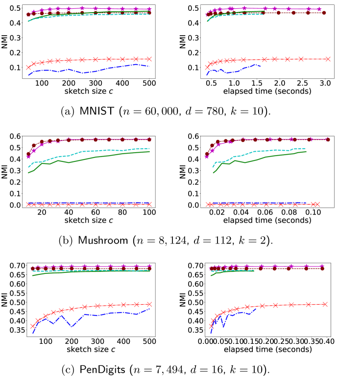
Figure 3: Comparisons between the runtimes and accuracies of approximate spectral clustering (SC) and approximate kernel $k$-means clustering (KK), both using uniform column sampling Nyström approximation.

Let ${\bf a}_{1},\ldots,{\bf a}_{n}\in{\mathbb{R}}^{d}$ be the input vectors. We take both the affinity matrix for spectral clustering and the kernel matrix for kernel $k$-means to be the RBF kernel matrix ${\bf K}=[\kappa({\bf a}_{i},{\bf a}_{j})]_{ij}\in{\mathbb{R}}^{n\times n}$, where $\kappa({\bf a},{\bf a}^{\prime})=\exp\big{(}-\frac{1}{2\sigma^{2}}\|{\bf a}-{\bf a}^{\prime}\|_{2}^{2}\big{)}$ and $\sigma$ is the kernel width parameter. We choose $\sigma$ based on the average interpoint distance in the data sets as

$$\sigma = \beta\cdot\sqrt{\textstyle\frac{1}{n^{2}}\sum_{i=1}^{n}\sum_{j=1}^{n}\|{\bf a}_{i}-{\bf a}_{j}\|_{2}^{2}},$$ (5)

where we take $\beta=0.2$, $1$, or $5$.

The algorithms under comparison are all implemented in Python 3.5.2. Our implementation of approximate spectral clustering follows the code in (Fowlkes et al., 2004). To compute linear $k$-means clusterings, we use the function sklearn.cluster.KMeans present in the scikit-learn package. Our algorithm for approximate kernel $k$-means clustering is described in more detail in Section 5.1. We ran the computations on a MacBook Pro with a 2.5GHz Intel Core i7 CPU and 16GB of RAM.

We compare approximate spectral clustering (SC) with approximate kernel $k$-means clustering (KK), with both using the rank-restricted Nyström method with uniform sampling. We used normalized mutual information (NMI) (Strehl and Ghosh, 2002) to evaluate clustering performance: the NMI falls between 0 (representing no mutual information between the true and approximate clusterings) and 1 (perfect correlation of the two clusterings), so larger NMI indicates better performance. The target dimension $s$ is taken to be $k$; and, for each method, the sketch size $c$ is varied from $5s$ to $50s$. We record the time cost of the two methods, excluding the time spent on the $k$-means clustering required in both algorithms. We repeat this procedure $100$ times and report the averaged NMI and average elapsed time.

We note that, at small sketch sizes $c$, exceptions often arise during approximate spectral clustering due to negative entries in the degree matrix. (This is an example, as discussed in Section 4.2, of when approximate spectral clustering heuristics do not perform well.) We discard the trials where such exceptions occur.

Our results are summarized in Figure 3. Figure 3 illustrates the NMI of SC and KK as a function of the sketch size $c$ and as a function of elapsed time for both algorithms. While there are quantitative differences between the results on the three data sets, the plots all show that KK is more accurate as a function of the sketch size or elapsed time than SC.

5 Single-Machine Medium-Scale Experiments

In this section, we empirically compare the Nyström method and random feature maps (Rahimi and Recht, 2007) for kernel $k$-means clustering. We conduct experiments on the data listed in Table 3. For the Mushrooms and PenDigits data, we are able to evaluate the objective function value of kernel $k$-means clustering.

Algorithm 2 Approximate Kernel $k$-Means Clustering using Nyström Approximation.

1:  Input: data set ${\bf a}_{1},\ldots,{\bf a}_{n}\in{\mathbb{R}}^{d}$, number of clusters $k$, target dimension $s$ ($\geq k$), arbitrary integer $\ell$ $(>s)$, sketch size $c$ ($>\ell$), kernel function $\kappa$.

2:  // Step 1: The Nyström Method

3:  Form sketches ${\bf C}={\bf K}{\bf P}\in{\mathbb{R}}^{n\times c}$ and ${\bf W}={\bf P}^{T}{\bf C}\in{\mathbb{R}}^{c\times c}$, where ${\bf K}=[\kappa({\bf a}_{i},{\bf a}_{j})]_{ij}\in{\mathbb{R}}^{n\times n}$ is the kernel matrix and ${\bf P}\in{\mathbb{R}}^{n\times c}$ is some sketching matrix, e.g., uniform sampling;

4:  Compute a matrix ${\bf R}\in{\mathbb{R}}^{n\times\ell}$ such that ${\bf R}{\bf R}^{T}={\bf C}{\bf W}_{\ell}^{-1}{\bf C}^{T}$;

5:  // Step 2: Dimensionality Reduction

6:  Compute the rank-$s$ truncated SVD ${\bf R}_{s}=\tilde{{\bf U}}_{s}\tilde{\mbox{\boldmath$\Sigma$\unboldmath}}_{s}\tilde{{\bf V}}_{s}^{T}$;

7:  Let ${\bf B}=\tilde{{\bf U}}_{s}\tilde{\mbox{\boldmath$\Sigma$\unboldmath}}_{s}(={\bf R}\tilde{{\bf V}}_{s})\in{\mathbb{R}}^{n\times s}$;

8:  // Step 3: Linear $k$-Means Clustering

9:  Perform $k$-means clustering over the rows of ${\bf B}$;

10:  return  the clustering results.

5.1 Single-Machine Implementation of Approximate Kernel $k$-Means

Our algorithm for approximate kernel $k$-means clustering comprises three steps: Nyström approximation, dimensionality reduction, and linear $k$-means clustering. Both the single-machine as well as the distributed variants of the algorithm are governed by three parameters: $s$, the number of features used in the clustering; $\ell$, a regularization parameter; and $c$, the sketch size. These parameters satisfy $k\leq s<\ell\leq c\ll n$.

1. Nyström approximation. Let $c$ be the sketch size and ${\bf P}\in{\mathbb{R}}^{n\times c}$ be a sketching matrix. Let ${\bf C}={\bf K}{\bf P}$ and ${\bf W}={\bf P}^{T}{\bf K}{\bf P}={\bf P}^{T}{\bf C}$. The standard Nyström approximation is ${\bf C}{\bf W}^{\dagger}{\bf C}^{T}$; small singular values in ${\bf W}$ can lead to instability in the Moore-Penrose inverse, so a widely used heuristic is to choose $\ell<c$ and use ${\bf C}{\bf W}_{\ell}^{-1}{\bf C}^{T}$ instead of the standard Nyström approximation. We set $\ell=\lceil c/2\rceil$ (arbitrarily). Let ${\bf W}_{\ell}={\bf U}_{{\bf W},\ell}\mbox{\boldmath$\Lambda$\unboldmath}_{{\bf W},\ell}{\bf U}_{{\bf W},\ell}^{T}$ be the truncated SVD of ${\bf W}$ and return ${\bf R}={\bf C}{\bf U}_{{\bf W},\ell}\mbox{\boldmath$\Lambda$\unboldmath}_{{\bf W},\ell}^{-1/2}\in{\mathbb{R}}^{n\times\ell}$ as the output of the Nyström method.

2. Dimensionality reduction. Let $\tilde{{\bf V}}_{s}\in{\mathbb{R}}^{\ell\times s}$ contain the dominant $s$ right singular vectors of ${\bf R}$. Let ${\bf B}={\bf R}\tilde{{\bf V}}_{s}\in{\mathbb{R}}^{n\times s}$. It can be verified that ${\bf B}{\bf B}^{T}=({\bf C}{\bf W}_{\ell}^{-1}{\bf C}^{T})_{s}$, which is our desired rank-restricted Nyström approximation.

3. Linear $k$-means clustering. With ${\bf B}\in{\mathbb{R}}^{n\times s}$ at hand, use an arbitrary off-the-shelf linear $k$-means clustering algorithm to cluster the rows of ${\bf B}$.

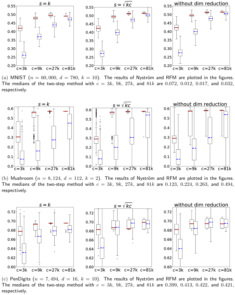
Figure 4: Quality of approximate kernel $k$-means clusterings using Nyström, random feature maps (Rahimi and Recht, 2007), and the two-step method (Chitta et al., 2011). (Dimensionality reduction is not applicable to the two-step method). The $y$-axis reports the normalized mutual information (NMI).

See Algorithm 2 for the single-machine version of this approximate kernel $k$-means clustering algorithm. Observe that we can use uniform sampling to form ${\bf C}$ and ${\bf W}$, and thereby avoid computing most of ${\bf K}$.

Let ${\bf R}\in{\mathbb{R}}^{n\times c}$ be the feature matrix computed by random feature maps (RFM). To make the comparison fair, we perform dimensionality reduction for RFM (Rahimi and Recht, 2007) in the same way as described in Algorithm 2 to compute ${\bf B}={\bf R}\tilde{{\bf V}}_{s}$, and apply linear $k$-means clustering on the rows of ${\bf B}$.

5.2 Comparing Nyström, Random Feature Maps, and Two-Step Method

We empirically compare the clustering performances of kernel approximations formed using Nyström, random feature map (RFM) (Rahimi and Recht, 2007), and the two-step method (Chitta et al., 2011) on the data sets detailed in Table 3.

We use the RBF kernel with width parameter given by (5); Figure 3 indicates that $\beta=1$ is a good choice for these data sets. We conduct dimensionality reduction for both Nyström and RFM to obtain $s$-dimensional features, and consider three choices: $s=k$, $s=\big{\lceil}\sqrt{ck}\big{\rceil}$, and without dimensionality reduction (equivalently, $s=c$).

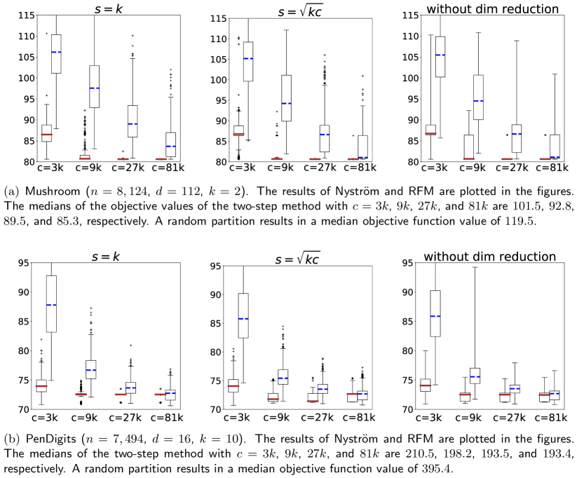
Figure 5: Quality of approximate kernel $k$-means clusterings obtained using rank-restricted Nyström, RFMs (Rahimi and Recht, 2007), and the two-step method (Chitta et al., 2011). (Dimensionality reduction is not applicable to the two-step method). The $y$-axis reports the kernel $k$-means clustering objective function value.

The quality of the clusterings is quantified using both normalized mutual information (NMI) (Strehl and Ghosh, 2002) and the objective function value:

$$\frac{1}{n}\>\sum_{i=1}^{k}\sum_{j\in{\mathcal{J}}_{i}}\bigg{\|}{\bf k}_{j}\>-\>\frac{1}{|{\mathcal{J}}_{i}|}\sum_{l\in{\mathcal{J}}_{i}}{\bf k}_{l}\bigg{\|}_{2}^{2},$$ (6)

where ${\bf k}_{1},\cdots,{\bf k}_{n}\in{\mathbb{R}}^{n}$ are the columns of the kernel matrix ${\bf K}$, and the disjoint sets ${\mathcal{J}}_{1},\cdots,{\mathcal{J}}_{k}$ reflect the clustering.

We repeat the experiments $500$ times and report the results in Figures 4 and 5. The experiments show that as measured by both NMIs and objective values, the Nyström method outperforms RFM in most cases. Both the Nyström method and RFM are consistently superior to the two-step method of (Chitta et al., 2011), which requires a large sketch size. All the compared methods improve as the sketch size $c$ increases.

Judging from these medium-scale experiments, the target rank $s$ has little impact on the NMI and clustering objective value. This phenomenon is not general; in the large-scale experiments of the next section we see that setting $s$ properly allows one to obtain a better NMI than an over-small or over-large $s$.

6 Large-Scale Experiments using Distributed Computing

In this section, we empirically study our approximate kernel $k$-means clustering algorithm on large-scale data. We state a distributed version of the algorithm, implement it in Apache Spark, and evaluate its performance on NERSC’s Cori supercomputer. We investigate the effect of increased parallelism, sketch size $c$, and target dimension $s$.

Algorithm 3 is a distributed version of our method described in Section 5.1. Again, we use uniform sampling to form ${\bf C}$ and ${\bf W}$ to avoid computing most of ${\bf K}$. We mainly focus on the Nyström approximation step, as the other two steps are well supported by distributed computing systems such as Apache Spark.

Algorithm 3 Distributed Approximate Kernel $k$-Means Clustering using Nyström Approximation.

1:  Input: data set ${\bf a}_{1},\ldots,{\bf a}_{n}\in{\mathbb{R}}^{d}$ distributed among $m$ machines, number of clusters $k$, target dimension $s$ ($\geq k$), arbitrary integer $\ell>s$, sketch size $c$ ($>\ell$), kernel function $\kappa$.

2:  // Step 1: The Nyström Method

3:  Sample $c$ vectors from ${\bf a}_{1},\ldots,{\bf a}_{n}$ to form ${\bf a}_{1}^{\prime},\ldots,{\bf a}_{c}^{\prime}$ and send to the driver;

4:  Driver computes ${\bf W}=[\kappa(a_{i}^{\prime},a_{j}^{\prime})]_{ij}\in{\mathbb{R}}^{c\times c}$ and a matrix ${\bf Z}\in{\mathbb{R}}^{c\times\ell}$ satisfying ${\bf Z}{\bf Z}^{T}={\bf W}_{\ell}^{-1}$;

5:  Broadcast ${\bf Z}$ and ${\bf a}_{1}^{\prime},\ldots,{\bf a}_{c}^{\prime}$ to all executors;

6:  for all $j\in[n]$ do

7:     Each executor locally computes ${\bf c}_{j}=[\kappa({\bf a}_{j},{\bf a}_{1}^{\prime});\ldots;\kappa({\bf a}_{j},{\bf a}_{c}^{\prime})]\in{\mathbb{R}}^{c}$ and ${\bf r}_{j}={\bf Z}^{T}{\bf c}_{j}\in{\mathbb{R}}^{\ell}$;

8:  end for

9:  // Step 2: Dimensionality Reduction

10:  Let $\tilde{{\bf V}}_{s}$ contain the dominant $s$ right singular vectors of the distributed row matrix ${\bf R}=[{\bf r}_{1},\ldots,{\bf r}_{n}]^{T}\in{\mathbb{R}}^{n\times\ell}$ (computed using a distributed truncated SVD algorithm);

11:  Broadcast $\tilde{{\bf V}}_{s}\in{\mathbb{R}}^{\ell\times s}$ to all executors;

12:  for all $j\in[n]$ do

13:     Each executor locally computes ${\bf b}_{j}=\tilde{{\bf V}}_{s}^{T}{\bf r}_{j}\in{\mathbb{R}}^{s}$;

14:  end for

15:  // Step 3: Linear $k$-Means Clustering

16:  Perform $k$-means clustering over the Nyström features ${\bf b}_{1},\ldots,{\bf b}_{n}\in{\mathbb{R}}^{s}$ (using a distributed linear $k$-means clustering algorithm).

17:  return  the clustering results.

Table 4: The mean and standard deviation of the runtimes of Algorithm 3, in seconds, as a function of the number of compute nodes. We report the total runtime as well as the runtimes of the three stages: Nyström approximation, dimensionality reduction (DR), and linear $k$-means clustering. The total time is the sum of the three stages and all the Spark overheads, e.g., Spark initialization. We fix $k=10$ and $c=400$. In the upper table, we set $s=20$, and the NMI is $0.400\pm 0.009$; in the lower table, we set $s=80$, and the NMI is $0.410\pm 0.010$.

	8 Nodes	16 Nodes	32 Nodes	64 Nodes	128 Nodes
Nyström	$2998.6\pm 263.9$	$1268.8\pm 106.4$	$665.2\pm 39.6$	$369.7\pm 126.1$	$181.4\pm 22.2$
DR	$37.4\pm 58.3$	$63.8\pm 72.5$	$38.9\pm 18.2$	$87.3\pm 37.8$	$183.9\pm 89.1$
$k$-means	$117.2\pm 132.3$	$153.1\pm 98.8$	$119.9\pm 76.9$	$223.2\pm 88.4$	$391.0\pm 155.9$
Total	$3201.5\pm 344.0$	$1532.0\pm 146.9$	$867.9\pm 97.5$	$734.7\pm 152.0$	$828.2\pm 210.4$

	8 Nodes	16 Nodes	32 Nodes	64 Nodes	128 Nodes
Nyström	$3008.4\pm 385.6$	$1312.9\pm 141.2$	$696.0\pm 111.8$	$342.5\pm 16.9$	$197.0\pm 24.1$
DR	$53.0\pm 41.9$	$58.7\pm 22.7$	$94.6\pm 31.8$	$179.4\pm 55.8$	$470.6\pm 118.5$
$k$-means	$58.2\pm 24.7$	$80.9\pm 31.8$	$104.6\pm 28.7$	$211.3\pm 103.1$	$501.7\pm 162.9$
Total	$3168.1\pm 434.1$	$1492.6\pm 135.3$	$940.6\pm 139.3$	$775.9\pm 151.6$	$1232.4\pm 232.1$

6.1 Experimental Setup

We implemented Algorithm 3 in the Apache Spark framework (Zaharia et al., 2010, 2012), using the Scala API. We computed the Nyström approximation using the matrix operations provided by Spark, and invoked the MLlib library for machine learning in Spark (Meng et al., 2016) to perform the dimensionality reduction and linear $k$-means clustering steps. For the linear $k$-means clustering, we set the maximum number of iterations to $100$.

We ran our experiments on Cori Phase I, a NERSC supercomputer, located at Lawrence Berkeley National Laboratory. Cori Phase I is a Cray XC40 system with 1632 compute nodes, each of which has two 2.3GHz 16-core Haswell processors and 128GB of DRAM. The Cray Aries high-speed interconnect linking the compute nodes is configured in a dragonfly topology.

We used the MNIST8M data set to conduct our empirical evaluations; this data set has $n=8.1\times 10^{6}$ instances, $d=784$ features, and $k=10$ clusters. We vary $c$ and $s$ and set $\ell=\frac{c}{2}$. We chose the RBF kernel width parameter according to (5) with $\beta=1.0$. We use Cori’s default setting of Spark configurations. For each setting of parameters, we repeated the experiments $10$ times and recorded the NMIs and elapsed time.

6.2 Effect of Increased Parallelism

We varied the number of nodes to test the impact of increased parallelism on each of the three steps in Algorithm 3. We set the sketch size to $c=400$ and the target dimension to $s=20$ or $80$. Table 4 reports the mean and standard deviation of the elapsed times. As a reference point, using $32$ nodes, our algorithm takes $15$ minutes on average to group the $8.1$ million input instances into $10$ clusters. We also plot the elapsed times in Figure 6.

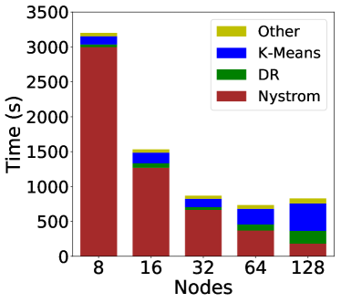
(a) $k=10$, $s=20$, $c=400$.

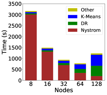
(b) $k=10$, $s=80$, $c=400$.

Figure 6: The mean of the runtimes of Algorithm 3, in seconds, as a function of the number of compute nodes.

The Nyström method scales very well with the increase of nodes: its elapsed time is inversely proportional to the number of nodes. This is because the Nyström method requires only 2 rounds of communications; the elapsed time is spent mostly on computation on the executors.

Dimensionality reduction (DR) and linear $k$-means clustering are highly iterative and thus have high latency, incur straggler delays, and have large scheduler and communication overheads. See (Gittens et al., 2016) for an in-depth discussion of the performance concerns when using Spark for distributed matrix computations. As the number of nodes increases from $32$ to $64$ and higher, DR and $k$-means exhibit anti-scaling behavior: as the number of nodes goes up, their runtimes increase rather than decrease. For DR, the input dimension is $\ell=\frac{c}{2}=200$, and the target dimension is $s=20$ or $80$; while for $k$-means, the input dimension is $s=20$ or $80$. Clearly, the issue here is not that DR and $k$-means are computationally intensive. Instead, as the number of nodes increase, although the per-node computational time decreases, the Spark communications overheads are increasing, making DR and $k$-means less performant. Such behavior has been characterized and studied in other Spark implementations of linear algebra algorithms (Gittens et al., 2016).

Table 5: The NMI and elapsed time (seconds) for varying sketch sizes $c$. Here “T” denotes the elapsed time. We use $32$ nodes. In the upper table, we set $s=20$; in the lower table, we set $s=80$.

	$c=100$	$c=400$	$c=1,600$
NMI	$0.3833\pm 0.0117$	$0.3975\pm 0.0112$	$0.4069\pm 0.0001$
T(Nyström)	$138.5\pm 62.1$	$665.2\pm 39.5$	$2634.5\pm 94.4$
T(DR)	$1.2\pm 0.5$	$38.9\pm 18.2$	$31.3\pm 6.6$
T($k$-Means)	$60.9\pm 28.7$	$119.9\pm 76.9$	$86.9\pm 27.3$
T(Total)	$227.4\pm 101.3$	$867.9\pm 97.5$	$2785.4\pm 83.2$

	$c=400$	$c=1600$
NMI	$0.4101\pm 0.0101$	$0.4233\pm 0.0131$
T(Nyström)	$696.0\pm 111.8$	$2728.1\pm 190.3$
T(DR)	$94.6\pm 31.8$	$97.9\pm 20.6$
T($k$-Means)	$104.6\pm 28.7$	$88.0\pm 23.9$
T(Total)	$940.6\pm 139.3$	$2952.2\pm 174.5$

6.3 Effect of Sketch Size $c$

We executed our Spark implementation using $32$ compute nodes, setting $s=20$ or $80$, and varying the target dimension $c$. Table 5 reports the observed normalized mutual information (NMI) (Strehl and Ghosh, 2002) and elapsed times. As predicted by our theory, for fixed $k$ and $s$, larger $c$ always leads to better performance.

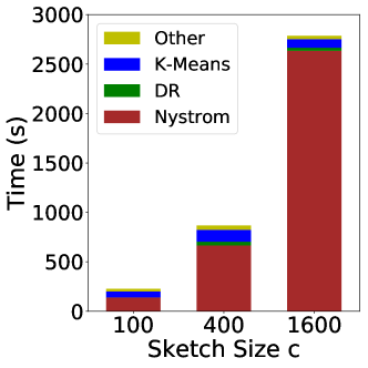
(a) $k=10$ and $s=20$.

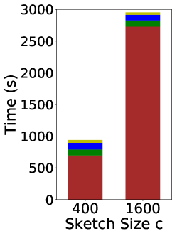
(b) $k=10$ and $s=80$.

Figure 7: The mean of the runtimes of Algorithm 3, in seconds, as a function of the sketch size $c$.

In Figure 7 we plot the runtime as a function of the sketch size $c$. The plots shows the significant influence of $c$ on the running time. In Figure 7, the runtime of Nyström grows superlinearly with $c$. According to our analysis, the computational and communication costs of Nyström are both superlinear in $c$. Therefore, the user should keep in mind this trade-off between the clustering performance and the computational cost.

6.4 Effect of Target Dimension $s$

We executed our Spark implementation using $32$ computational nodes, fixing $k=10$ and $c=1600$ and varying the target dimension $s$. Table 6 reports the observed NMIs and elapsed times. For fixed $k$ and $c$, a moderately large $s$ leads to better clustering performance. However, as $s$ grows, $\tfrac{k}{s}$ decreases but $\tfrac{s}{c}$ increases, so as predicted in Remark 3, the clustering performance is nonmonotonic in $s$. Indeed, as $s$ grows from $80$ to $160$, the NMI deteriorates. In practice, for fixed $k$ and $c$, one should set $s$ moderately large, but not over-large.

Table 6: The NMI and elapsed time (seconds) for varying target dimensions $s$. Here “T” denotes the elapsed time. We use $32$ nodes and fix $c=1600$.

	$s=10$	$s=20$	$s=40$	$s=80$	$s=160$	$s=320$
NMI	$0.3852\pm 0.0003$	$0.4069\pm 0.0001$	$0.4130\pm 0.0062$	$0.4233\pm 0.0131$	$0.4086\pm 0.0125$	$0.4099\pm 0.0098$
T(Nyström)	$2702.2\pm 131.6$	$2634.5\pm 94.4$	$2815.3\pm 403.6$	$2728.1\pm 190.3$	$2849.9\pm 511.2$	$2757.1\pm 271.9$
T(DR)	$21.1\pm 3.2$	$31.3\pm 6.6$	$57.5\pm 9.2$	$97.9\pm 20.6$	$168.2\pm 29.0$	$570.5\pm 151.0$
T($k$-Means)	$84.0\pm 6.4$	$86.9\pm 27.3$	$90.6\pm 9.0$	$88.0\pm 23.9$	$99.8\pm 12.2$	$169.3\pm 64.2$
T(Total)	$2840.9\pm 132.0$	$2785.4\pm 83.2$	$3003.4\pm 413.7$	$2952.2\pm 174.5$	$3157.5\pm 549.2$	$3537.5\pm 256.3$

In Figure 8 we plot the runtime as a function of the target dimension $s$. Note that $s$ does not affect the time cost of the Nyström method. As $s$ grows, the time costs of dimensionality reduction and linear $k$-means clustering both increase. This implies that a moderate $s$ is good for computational purpose. Previously, in Figure 2, we plot the NMI as a function of $s$ while fixing $k$ and $c$. Figure 2 shows that a proper $s$ leads to better NMI than an over-large or over-small $s$. In sum, setting $s$ properly has both computational and accuracy benefits, which corroborates our theory.

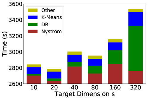
Figure 8: The mean of the runtimes of Algorithm 3, in seconds, as a function of the target dimension $s$. We use $32$ nodes and fix $k=10$ and $c=1600$.

7 Conclusion

We provided principled algorithms for computing approximate kernel $k$-means clusterings. In particular, we showed that the combination of linear $k$-means with rank-restricted Nyström approximation is theoretically sound, practically useful, and scalable to large data sets. This should be contrasted with approximate spectral clustering using Nyström approximation. Although the latter is a widely-used approach to scalable non-linear clustering, it has theoretical deficiencies and practical limitations. Experiments demonstrated that approximate kernel $k$-means clustering using the rank-restricted Nyström approximation consistently outperforms approximate spectral clustering.

Our analysis uses the concept of projection-cost preservation and builds upon the existing theory of randomized linear algebra. Our main result is a $1+\epsilon$ approximation ratio guarantee for kernel $k$-means clustering: when $s=\frac{k}{\epsilon}$ Nyström features are used, a $1+{\mathcal{O}}(\epsilon)$ approximation ratio is guaranteed with high probability. As an intermediate theoretical result of independent interest, we introduced a novel rank-restricted Nyström approximation and proved that it gives a $1+\epsilon$ relative-error low-rank approximation guarantee in the trace norm.

To complement our theory, we investigated the performance of the rank-restricted Nyström approximation when applied to kernel $k$-means clustering. We produced an Apache Spark implementation of a distributed version of our approximate kernel $k$-means algorithm, and applied it to cluster 8.1 million vectors; the results demonstrate the usefulness and simplicity of kernel $k$-means with rank-restricted Nyström approximation for clustering moderately large-scale data sets. Combined with recent work on user-friendly frameworks for distributed computing systems (Zaharia et al., 2010, 2012), large-scale machine learning (Meng et al., 2016), and large-scale randomized linear algebra (Gittens et al., 2016), our results suggest the use of kernel $k$-means with rank-restricted Nyström approximations for simple, computationally efficient, and theoretically principled clustering of large-scale data sets.

Acknowledgments

We thank the authors of Musco and Musco (2017) for bringing to our attention their results on approximate kernel $k$-means clustering through the use of ridge leverage score Nyström approximations, the authors of Tropp et al. (2017) for informing us of their contemporaneous guarantees on the approximation error of rank-restricted Nyström approximations, and the anonymous reviewers for their helpful suggestions. We would like to acknowledge ARO, DARPA, NSF, and ONR for providing partial support of this work.

A Proof of Theorem 1

In this section, we will provide a proof of Theorem 1, our main quality-of-approximation result for rank-restricted Nyström approximation. We will start, in Section A.1, by establishing three technical lemmas; then, in Section A.2, we will establish an important structural result on the rank-restricted Nyström approximation as well as key approximate matrix multiplication properties for low-rank matrix approximation; and finally, in Section A.3, we will use these results to prove Theorem 1.

A.1 Technical Lemmas

Lemma 5 is a very well known result. See (Boutsidis et al., 2014; Zhang, 2015). Here we offer a simplified proof.

Lemma 5

Let ${\bf A}\in{\mathbb{R}}^{n\times m}$ be any matrix and ${\bf U}\in{\mathbb{R}}^{n\times c}$ have orthonormal columns. Let $s$ be any positive integer no greater than $c$. Then

$$({\bf U}^{T}{\bf A})_{s}\;=\;\mathop{\rm argmin}_{\mathrm{rank}({\bf Z})\leq s}\big{\|}{\bf A}-{\bf U}{\bf Z}\big{\|}_{F}^{2}.$$

Proof  Let ${\bf U}^{\perp}\in{\mathbb{R}}^{n\times(n-c)}$ be the orthogonal complement of ${\bf U}$. It holds that

$$\Big{\|}{\bf A}-{\bf U}{\bf Z}\Big{\|}_{F}^{2} = \Bigg{\|}{\bf A}\,-\,\left[\begin{array}[]{cc}{\bf U}&{\bf U}^{\perp}\\ \end{array}\right]\left[\begin{array}[]{c}{\bf Z}\\ {\bf 0}\\ \end{array}\right]\Bigg{\|}_{F}^{2}$$

$$= \Bigg{\|}\left[\begin{array}[]{c}{\bf U}^{T}\\ ({\bf U}^{\perp})^{T}\\ \end{array}\right]\,{\bf A}\,-\,\left[\begin{array}[]{c}{\bf Z}\\ {\bf 0}\\ \end{array}\right]\Bigg{\|}_{F}^{2}$$

$$= \Bigg{\|}\left[\begin{array}[]{cc}{\bf U}^{T}{\bf A}-{\bf Z}\\ ({\bf U}^{\perp})^{T}{\bf A}\\ \end{array}\right]\Bigg{\|}_{F}^{2}$$

$$= \big{\|}{\bf U}^{T}{\bf A}-{\bf Z}\big{\|}_{F}^{2}+\big{\|}({\bf U}^{\perp})^{T}{\bf A}\big{\|}_{F}^{2},$$

where the second equality follows from the unitary invariance of the Frobenius norm. Then

$$\mathop{\rm argmin}_{\mathrm{rank}({\bf Z})\leq s}\big{\|}{\bf A}-{\bf U}{\bf Z}\big{\|}_{F}^{2}\;=\;\mathop{\rm argmin}_{\mathrm{rank}({\bf Z})\leq s}\big{\|}{\bf U}^{T}{\bf A}-{\bf Z}\big{\|}_{F}^{2}\;=\;({\bf U}^{T}{\bf A})_{s},$$

by which the lemma follows.  

Lemma 6 is a new result established in this work. The lemma plays an important role in analyzing the rank-restricted Nyström method.

Lemma 6

Let ${\bf A}\in{\mathbb{R}}^{n\times m}$ be any matrix and ${\bf U}\in{\mathbb{R}}^{n\times c}$ has orthonormal columns. Let $s\leq c$ be arbitrary integer. Let ${\bf Q}\in{\mathbb{R}}^{n\times s}$ be the orthonormal bases of the rank $s$ matrix ${\bf U}({\bf U}^{T}{\bf A})_{s}\in{\mathbb{R}}^{n\times m}$. Then ${\bf Q}{\bf Q}^{T}{\bf A}={\bf U}({\bf U}^{T}{\bf A})_{s}$.

Proof  Let ${\bf Z}^{\star}={\bf Q}^{T}{\bf U}({\bf U}^{T}{\bf A})_{s}\in{\mathbb{R}}^{s\times m}$. By the definition of ${\bf Q}$, we have

$${\bf Q}{\bf Q}^{T}{\bf U}({\bf U}^{T}{\bf A})_{s}\;=\;{\bf U}({\bf U}^{T}{\bf A})_{s}.$$ (10)

It holds that

$$\big{\|}{\bf U}({\bf U}^{T}{\bf A})_{s}-{\bf A}\big{\|}_{F}^{2}\;=\;\min_{\mathrm{rank}({\bf X})\leq s}\big{\|}{\bf U}{\bf X}-{\bf A}\big{\|}_{F}^{2}\;\leq\;\min_{\mathrm{rank}({\bf Z})\leq s}\big{\|}{\bf Q}{\bf Z}-{\bf A}\big{\|}_{F}^{2}\;\leq\;\big{\|}{\bf Q}{\bf Z}^{\star}-{\bf A}\big{\|}_{F}^{2},$$

where the equality follows from Lemma 5; the former inequality follows from that $\mathrm{range}({\bf Q})\subset\mathrm{range}({\bf U})$. Because ${\bf U}({\bf U}^{T}{\bf A})_{s}={\bf Q}{\bf Z}^{\star}$ by (10), the lefthand and righthand sides are equal, and thereby

$$\min_{\mathrm{rank}({\bf Z})\leq s}\big{\|}{\bf Q}{\bf Z}-{\bf A}\big{\|}_{F}^{2}\;=\;\big{\|}{\bf Q}{\bf Z}^{\star}-{\bf A}\big{\|}_{F}^{2}.$$

Since ${\bf Z}$ is $s\times m$, it follows that

$$\min_{{\bf Z}}\big{\|}{\bf Q}{\bf Z}-{\bf A}\big{\|}_{F}^{2}\;=\;\min_{\mathrm{rank}({\bf Z})\leq s}\big{\|}{\bf Q}{\bf Z}-{\bf A}\big{\|}_{F}^{2}\;=\;\big{\|}{\bf Q}{\bf Z}^{\star}-{\bf A}\big{\|}_{F}^{2}.$$ (11)

Let ${\bf Q}^{\perp}\in{\mathbb{R}}^{n\times(n-s)}$ be the orthogonal complement of ${\bf Q}$. It holds that

$$\Big{\|}{\bf A}-{\bf Q}{\bf Z}\Big{\|}_{F}^{2} = \Bigg{\|}{\bf A}\,-\,\left[\begin{array}[]{cc}{\bf Q}&{\bf Q}^{\perp}\\ \end{array}\right]\left[\begin{array}[]{c}{\bf Z}\\ {\bf 0}\\ \end{array}\right]\Bigg{\|}_{F}^{2}$$

$$= \Bigg{\|}\left[\begin{array}[]{c}{\bf Q}^{T}\\ ({\bf Q}^{\perp})^{T}\\ \end{array}\right]\,{\bf A}\,-\,\left[\begin{array}[]{c}{\bf Z}\\ {\bf 0}\\ \end{array}\right]\Bigg{\|}_{F}^{2}$$

$$= \Bigg{\|}\left[\begin{array}[]{cc}{\bf Q}^{T}{\bf A}-{\bf Z}\\ ({\bf Q}^{\perp})^{T}{\bf A}\\ \end{array}\right]\Bigg{\|}_{F}^{2}$$

$$= \big{\|}{\bf Q}^{T}{\bf A}-{\bf Z}\big{\|}_{F}^{2}+\big{\|}({\bf Q}^{\perp})^{T}{\bf A}\big{\|}_{F}^{2},$$

where the second equality follows from the unitary invariance of the Frobenius norm. Obviously, ${\bf Z}={\bf Q}^{T}{\bf A}$ is the unique minimizer of $\min_{\bf Z}\|{\bf Q}{\bf Z}-{\bf A}\|_{F}^{2}$; otherwise ${\bf Q}^{T}{\bf A}-{\bf Z}$ in the righthand side is non-zero, making the objective function increase.

On the one hand, Eqn. (11) shows that ${\bf Z}^{\star}={\bf Q}^{T}{\bf U}({\bf U}^{T}{\bf A})_{s}\in{\mathbb{R}}^{s\times m}$ is one minimizer of $\min_{{\bf Z}}\|{\bf Q}{\bf Z}-{\bf A}\|_{F}^{2}$. On the other hand, we have that ${\bf Z}={\bf Q}^{T}{\bf A}$ is the unique minimizer of $\min_{\bf Z}\|{\bf Q}{\bf Z}-{\bf A}\|_{F}^{2}$. By the uniqueness, we have

$${\bf Z}^{\star}\;=\;{\bf Q}^{T}{\bf U}({\bf U}^{T}{\bf A})_{s}\;=\;{\bf Q}^{T}{\bf A}.$$

It follows that

$${\bf Q}{\bf Q}^{T}{\bf U}({\bf U}^{T}{\bf A})_{s}\;=\;{\bf Q}{\bf Q}^{T}{\bf A}.$$

The lemma follows from (10) and the above equality.  

Lemma 7 is a new result established by this work. Let ${\bf A}$ be any symmetric matrix. Lemma 7 analyzes the power scheme: using ${\bf A}^{t}{\bf P}$, instead of ${\bf A}{\bf P}$, as a sketch of ${\bf A}$. The lemma shows that the power scheme leads to an improvement of $\big{(}\frac{\sigma_{s+1}^{2}}{\sigma_{s}^{2}}\big{)}^{t-1}$, where $\sigma_{i}$ is the $i$-th biggest singular value of ${\bf A}$. Lemma 7 with $t=1$ is identical to (Boutsidis et al., 2014, Lemma 9). The power scheme has been studied by Gittens and Mahoney (2016); Halko et al. (2011); Woodruff (2014); their results do not allow the rank restriction $\mathrm{rank}({\bf X})\leq s$. To prove Theorem 1, we only need $t=1$; we will use Lemma 7 to extend Theorem 1 to the power method.

Lemma 7

Let ${\bf A}\in{\mathbb{R}}^{n\times n}$ be any SPSD matrix and ${\bf A}_{s}={\bf V}_{s}\mbox{\boldmath$\Sigma$\unboldmath}_{s}{\bf V}_{s}^{T}$ be the truncated SVD. Let ${\bf P}\in{\mathbb{R}}^{n\times c}$ satisfy that ${\bf P}^{T}{\bf V}_{s}\in{\mathbb{R}}^{c\times s}$ has full column rank. Let $t\geq 1$ be any integer and ${\bf C}={\bf A}^{t}{\bf P}$. Then for $\xi=2$ or $F$,

$$\min_{\mathrm{rank}({\bf X})\leq s}\big{\|}{\bf A}-{\bf C}{\bf X}\big{\|}_{\xi}^{2} \leq \big{\|}{\bf A}-{\bf A}_{s}\big{\|}_{\xi}^{2}+\big{(}\tfrac{\sigma_{s+1}^{2}}{\sigma_{s}^{2}}\big{)}^{t-1}\big{\|}({\bf A}-{\bf A}_{s}){\bf P}({\bf V}_{s}^{T}{\bf P})^{\dagger}\big{\|}_{\xi}^{2},$$

where $\sigma_{i}$ is the $i$-th largest singular value of ${\bf A}$.

Proof  We construct the rank $s$ matrix $\tilde{{\bf A}}_{s}={\bf C}({\bf V}_{s}^{T}{\bf P})^{\dagger}\mbox{\boldmath$\Sigma$\unboldmath}_{s}^{1-t}{\bf V}_{s}^{T}$ and use it to facilitate our proof. Since $\tilde{{\bf A}}_{s}$ has rank $s$, and its column space is in $\mathrm{range}({\bf C})$, it holds that

$$\min_{\mathrm{rank}({\bf X})\leq s}\big{\|}{\bf A}-{\bf C}{\bf X}\big{\|}_{\xi}^{2}\;\leq\;\big{\|}{\bf A}-\tilde{{\bf A}}_{s}\big{\|}_{\xi}^{2}$$

$$=\;\big{\|}({\bf A}-{\bf A}_{s})+({\bf A}_{s}-\tilde{{\bf A}}_{s})\big{\|}_{\xi}^{2}\;\leq\;\big{\|}{\bf A}-{\bf A}_{s}\big{\|}_{\xi}^{2}+\big{\|}{\bf A}_{s}-\tilde{{\bf A}}_{s}\big{\|}_{\xi}^{2}.$$

The latter inequality follows from that the row space of ${\bf A}_{s}-\tilde{{\bf A}}_{s}$ is in $\mathrm{range}({\bf V}_{s})$, that $({\bf A}-{\bf A}_{s}){\bf V}_{s}={\bf 0}$, and the matrix Pythagorean theorem. By the assumption $\mathrm{rank}({\bf V}_{s}^{T}{\bf P})=s$, it holds that $({\bf V}_{s}^{T}{\bf P})({\bf V}_{s}^{T}{\bf P})^{\dagger}={\bf I}_{s}$. We have

$$\big{\|}{\bf A}_{s}-\tilde{{\bf A}}_{s}\big{\|}_{\xi}^{2}\;=\;\big{\|}{\bf A}_{s}-({\bf A}_{s}^{t}+{\bf A}^{t}-{\bf A}_{s}^{t}){\bf P}({\bf V}_{s}^{T}{\bf P})^{\dagger}\mbox{\boldmath$\Sigma$\unboldmath}_{s}^{1-t}{\bf V}_{s}^{T}\big{\|}_{\xi}^{2}$$

$$=\;\big{\|}{\bf A}_{s}-{\bf V}_{s}\mbox{\boldmath$\Sigma$\unboldmath}_{s}^{t}\underbrace{({\bf V}_{s}^{T}{\bf P})}_{s\times c}\underbrace{({\bf V}_{s}^{T}{\bf P})^{\dagger}}_{c\times s}\mbox{\boldmath$\Sigma$\unboldmath}_{s}^{1-t}{\bf V}_{s}^{T}-({\bf A}^{t}-{\bf A}_{s}^{t}){\bf P}({\bf V}_{s}^{T}{\bf P})^{\dagger}\mbox{\boldmath$\Sigma$\unboldmath}_{s}^{1-t}{\bf V}_{s}^{T}\big{\|}_{\xi}^{2}$$

$$=\;\big{\|}{\bf A}_{s}-{\bf V}_{s}\mbox{\boldmath$\Sigma$\unboldmath}_{s}{\bf V}_{s}^{T}-({\bf A}^{t}-{\bf A}_{s}^{t}){\bf P}({\bf V}_{s}^{T}{\bf P})^{\dagger}\mbox{\boldmath$\Sigma$\unboldmath}_{s}^{1-t}{\bf V}_{s}^{T}\big{\|}_{\xi}^{2}$$

$$=\;\big{\|}({\bf A}^{t}-{\bf A}_{s}^{t}){\bf P}({\bf V}_{s}^{T}{\bf P})^{\dagger}\mbox{\boldmath$\Sigma$\unboldmath}_{s}^{1-t}{\bf V}_{s}^{T}\big{\|}_{\xi}^{2}$$

$$\leq\;\big{\|}({\bf A}-{\bf A}_{s})^{t-1}\big{\|}_{2}^{2}\big{\|}\mbox{\boldmath$\Sigma$\unboldmath}_{s}^{1-t}\big{\|}_{2}^{2}\big{\|}({\bf A}-{\bf A}_{s}){\bf P}({\bf V}_{s}^{T}{\bf P})^{\dagger}\big{\|}_{\xi}^{2}$$

$$=\;\big{(}\tfrac{\sigma_{s+1}^{2}}{\sigma_{s}^{2}}\big{)}^{t-1}\big{\|}({\bf A}-{\bf A}_{s}){\bf P}({\bf V}_{s}^{T}{\bf P})^{\dagger}\big{\|}_{\xi}^{2},$$

by which the lemma follows.  

A.2 Structural Result and Approximate Matrix Multiplication Properties

Lemma 8 is a structural result of independent interest that is important for establishing Theorem 1. By structural result, we mean that it is a linear algebraic result that holds for any matrix ${\bf P}$, and in particular for any matrix ${\bf P}$ that is a randomized sketching matrix. In particular, given this structural result, randomness in an algorithm enters only via ${\bf P}$. The importance of establishing such structural results within randomized linear algebra has been highlighted previously (Drineas et al., 2011; Mahoney, 2011; Gittens and Mahoney, 2016; Mahoney and Drineas, 2016; Wang et al., 2017).

Lemma 8

Let ${\bf K}\in{\mathbb{R}}^{n\times n}$ be any SPSD matrix, ${\bf P}\in{\mathbb{R}}^{n\times c}$ be any matrix, and $s\leq c$ be any positive integer. Let ${\bf D}={\bf K}^{1/2}{\bf P}\in{\mathbb{R}}^{n\times c}$, $\rho=\mathrm{rank}({\bf D})\leq c$, and ${\bf U}\in{\mathbb{R}}^{n\times\rho}$ be the left singular vectors of ${\bf D}$. Let ${\bf Q}\in{\mathbb{R}}^{n\times s}$ be any orthonormal bases of ${\bf U}({\bf U}^{T}{\bf K}^{1/2})_{s}$. It holds that

$$\big{(}{\bf C}{\bf W}^{\dagger}{\bf C}^{T}\big{)}_{s} = {\bf K}^{1/2}{\bf Q}{\bf Q}^{T}{\bf K}^{1/2},$$

$$\big{\|}{\bf K}-\big{(}{\bf C}{\bf W}^{\dagger}{\bf C}^{T}\big{)}_{s}\big{\|}_{*} = \min_{\mathrm{rank}({\bf Z})\leq s}\big{\|}{\bf K}^{1/2}-({\bf K}^{1/2}{\bf P}){\bf Z}\big{\|}_{F}^{2}.$$

Proof  Let ${\bf D}={\bf K}^{1/2}{\bf P}={\bf U}\mbox{\boldmath$\Sigma$\unboldmath}{\bf V}^{T}\in{\mathbb{R}}^{n\times c}$ be the SVD of ${\bf D}$. It holds that ${\bf C}={\bf K}{\bf P}={\bf K}^{1/2}{\bf D}$ and ${\bf W}={\bf P}^{T}{\bf K}{\bf P}={\bf D}^{T}{\bf D}$. It follows the SVD of ${\bf D}$ that

$${\bf C}({\bf W}^{\dagger})^{1/2}\;=\;{\bf K}^{1/2}{\bf D}\big{(}({\bf D}^{T}{\bf D})^{\dagger}\big{)}^{1/2}\;=\;{\bf K}^{1/2}({\bf U}\mbox{\boldmath$\Sigma$\unboldmath}{\bf V}^{T})\big{(}{\bf V}\mbox{\boldmath$\Sigma$\unboldmath}^{-2}{\bf V}^{T}\big{)}^{1/2}\;=\;{\bf K}^{1/2}{\bf U}{\bf V}^{T}.$$

We need the following lemma to prove Lemma 8. The following lemma is not hard to prove.

Lemma 9

Let the integers $n,c,\rho,s$ satisfy $n\geq c\geq\rho\geq s$. Let ${\bf A}\in{\mathbb{R}}^{n\times\rho}$ be any matrix with rank at least $s$ and ${\bf V}\in{\mathbb{R}}^{c\times\rho}$ has orthonormal columns. Then $({\bf A}{\bf V}^{T})_{s}={\bf A}_{s}{\bf V}^{T}$.

If $\mathrm{rank}({\bf K}^{1/2}{\bf U})<s$, then obviously ${\bf K}^{1/2}{\bf U}{\bf V}^{T}=({\bf K}^{1/2}{\bf U}{\bf V}^{T})_{s}=({\bf K}^{1/2}{\bf U})_{s}{\bf V}^{T}$. We thus assume $\mathrm{rank}({\bf K}^{1/2}{\bf U}{\bf V}^{T})\geq s$ and can apply the above lemma to show $({\bf K}^{1/2}{\bf U}{\bf V}^{T})_{s}=({\bf K}^{1/2}{\bf U})_{s}{\bf V}^{T}$. In either case, we have

$$({\bf K}^{1/2}{\bf U}{\bf V}^{T})_{s}\;=\;({\bf K}^{1/2}{\bf U})_{s}{\bf V}^{T}.$$

It follows from (A.2) that $\big{(}{\bf C}({\bf W}^{\dagger})^{1/2}\big{)}_{s}=({\bf K}^{1/2}{\bf U})_{s}{\bf V}^{T}$. Thus

$$\big{(}{\bf C}{\bf W}^{\dagger}{\bf C}^{T}\big{)}_{s}\;=\;({\bf K}^{1/2}{\bf U})_{s}({\bf U}^{T}{\bf K}^{1/2})_{s}\;=\;({\bf K}^{1/2}{\bf U})_{s}{\bf U}^{T}{\bf U}({\bf U}^{T}{\bf K}^{1/2})_{s}$$

Let ${\bf Q}\in{\mathbb{R}}^{n\times s}$ be the orthonormal bases of the rank $s$ matrix ${\bf U}({\bf U}^{T}{\bf K}^{1/2})_{s}$. Lemma 6 ensures that

$${\bf Q}{\bf Q}^{T}{\bf K}^{1/2}\;=\;{\bf U}({\bf U}^{T}{\bf K}^{1/2})_{s}.$$

It follows that

$$\big{(}{\bf C}{\bf W}^{\dagger}{\bf C}^{T}\big{)}_{s}\;=\;{\bf K}^{1/2}{\bf Q}{\bf Q}^{T}{\bf K}^{1/2},$$ (15)

by which the former conclusion of the lemma follows.

It is well known that $\|{\bf Y}\|_{*}=\mathrm{tr}({\bf Y})$ for any SPSD matrix ${\bf Y}$ and that $\mathrm{tr}({\bf A}^{T}{\bf A})=\|{\bf A}\|_{F}^{2}$ for any matrix ${\bf A}$. It follows from (15) that

$$\big{\|}{\bf K}-\big{(}{\bf C}{\bf W}^{\dagger}{\bf C}^{T}\big{)}_{s}\big{\|}_{*}\;=\;\big{\|}{\bf K}^{1/2}\big{(}{\bf I}_{n}-{\bf Q}{\bf Q}^{T}\big{)}{\bf K}^{1/2}\big{\|}_{*}$$

$$=\;\mathrm{tr}\Big{(}{\bf K}^{1/2}\big{(}{\bf I}_{n}-{\bf Q}{\bf Q}^{T}\big{)}\big{(}{\bf I}_{n}-{\bf Q}{\bf Q}^{T}\big{)}{\bf K}^{1/2}\Big{)}$$

$$=\;\big{\|}\big{(}{\bf I}_{n}-{\bf Q}{\bf Q}^{T}\big{)}{\bf K}^{1/2}\big{\|}_{F}^{2}\;=\;\big{\|}{\bf K}^{1/2}-{\bf U}({\bf U}^{T}{\bf K}^{1/2})_{s}\big{\|}_{F}^{2};$$

here the second equality holds because ${\bf K}^{1/2}({\bf I}_{n}-{\bf Q}{\bf Q}^{T}){\bf K}^{1/2}$ is SPSD and $({\bf I}_{n}-{\bf Q}{\bf Q}^{T})$ is orthogonal projection matrix; the last equality follows from Lemma 6. It follows from Lemma 5 that

$$\big{\|}{\bf K}-\big{(}{\bf C}{\bf W}^{\dagger}{\bf C}^{T}\big{)}_{s}\big{\|}_{*}\;=\;\big{\|}{\bf K}^{1/2}-{\bf U}({\bf U}^{T}{\bf K}^{1/2})_{s}\big{\|}_{F}^{2}$$

$$=\;\min_{\mathrm{rank}({\bf X})\leq s}\big{\|}{\bf K}^{1/2}-{\bf U}{\bf X}\big{\|}_{F}^{2}\;=\;\min_{\mathrm{rank}({\bf Z})\leq s}\big{\|}{\bf K}^{1/2}-{\bf D}{\bf Z}\big{\|}_{F}^{2},$$

by which the latter conclusion of the lemma follows.  

Lemma 10 formally defines the key approximate matrix multiplication properties (subspace embedding property and approximate orthogonality property) which—when sketching dimensions are chosen appropriately (see Table 7)—are shared by the uniform sampling, leverage score sampling, Gaussian projection, SRHT, and CountSketch sketching methods. Establishing approximate matrix multiplication bounds is the key step in proving many approximate regression and low-rank approximation results (Mahoney, 2011), and this lemma will be used crucually in the proof of Theorem 1.

Lemma 10 (Key Approximate Matrix Multiplication Properties for a Sketch)

Let $\eta,\epsilon,\delta_{1},\delta_{2}\in(0,1)$ be fixed parameters. Fix ${\bf Y}\in{\mathbb{R}}^{n\times d}$ and let ${\bf V}\in{\mathbb{R}}^{n\times s}$ have orthonormal columns. Let ${\bf P}\in{\mathbb{R}}^{n\times c}$ be one of the sketching methods listed in Table 7. When $c$ is larger than the quantity in the middle column of the corresponding row of Table 7, the subspace embedding property

$$\big{\|}{\bf V}^{T}{\bf P}{\bf P}^{T}{\bf V}-{\bf I}_{s}\big{\|}_{2}\;\leq\;\eta$$

holds with probability at least $1-\delta_{1}$. When $c$ is larger than the quantity in the right-hand column of the corresponding row of Table 7, the matrix multiplication property

$$\big{\|}{\bf V}^{T}{\bf P}{\bf P}^{T}{\bf Y}-{\bf V}^{T}{\bf Y}\big{\|}_{F}^{2}\;\leq\;\epsilon\|{\bf Y}\|_{F}^{2}$$

holds with probability at least $1-\delta_{2}$.

Table 7: Sufficient sketching dimensions for the sketching properties of Lemma 10 to hold. The leverage score sampling referred to here is with respect to the leverage scores of the matrix ${\bf V}$ described in Lemma 10. Similarly, $\mu$ is the row coherence of ${\bf V}$.

Sketching	Subspace Embedding	Matrix Multiplication
Leverage Score Sampling	$\frac{s}{\eta^{2}}\log\frac{s}{\delta_{1}}$	$\frac{s}{\epsilon\delta_{2}}$
Uniform Sampling	$\frac{\mu s}{\eta^{2}}\log\frac{s}{\delta_{1}}$	$\frac{\mu s}{\epsilon\delta_{2}}$
SRHT	$\frac{s+\log n}{\eta^{2}}\log\frac{s}{\delta_{1}}$	$\frac{s+\log n}{\epsilon\delta_{2}}$
Gaussian Projection	$\frac{s+\log(1/\delta_{1})}{\eta^{2}}$	$\frac{s}{\epsilon\delta_{2}}$
CountSketch	$\frac{s^{2}}{\delta_{1}\eta^{2}}$	$\frac{s}{\epsilon\delta_{2}}$

Proof  This lemma is a reproduction of (Wang et al., 2016b, Lemma 2), and is a collation of heterogenously stated results from the literature. The random sampling estimates were established by Drineas et al. (2008); Wang et al. (2016a); Woodruff (2014). The Gaussian projection was firstly analyzed by Johnson and Lindenstrauss (1984); see Woodruff (2014) for a proof of the stated sufficient sketching dimensions. The SRHT estimates are from Drineas et al. (2011); Lu et al. (2013); Tropp (2011). The CountSketch estimates are from Meng and Mahoney (2013); Nelson and Nguyên (2013).  

A.3 Completing the Proof of Theorem 1

Proof  Let ${\bf K}_{s}={\bf V}_{s}\mbox{\boldmath$\Lambda$\unboldmath}_{s}{\bf V}_{s}^{T}\in{\mathbb{R}}^{n\times n}$ be the truncated SVD of ${\bf K}$. It follows from Lemma 10 and the sketch sizes defined in Table 2 that

$$\big{\|}{\bf V}_{s}^{T}{\bf P}{\bf P}^{T}{\bf V}_{s}-{\bf I}_{s}\big{\|}_{2} \leq \eta,$$

$$\big{\|}({\bf K}^{1/2}-{\bf K}_{s}^{1/2}){\bf P}{\bf P}^{T}{\bf V}_{s}\big{\|}_{F}^{2} \leq \epsilon\big{\|}{\bf K}^{1/2}-{\bf K}_{s}^{1/2}\|_{F}^{2}$$

hold simultaneously with probability at least $0.9$.

It follows from Lemma 8 that

$$\big{\|}{\bf K}-\big{(}{\bf C}{\bf W}^{\dagger}{\bf C}^{T}\big{)}_{s}\big{\|}_{*}\;=\;\min_{\mathrm{rank}({\bf Z})\leq s}\big{\|}{\bf K}^{1/2}-({\bf K}^{1/2}{\bf P}){\bf Z}\big{\|}_{F}^{2}$$

$$\leq\;\big{\|}{\bf K}^{1/2}-{\bf K}_{s}^{1/2}\big{\|}_{F}^{2}+\big{\|}({\bf K}^{1/2}-{\bf K}_{s}^{1/2}){\bf P}({\bf V}_{s}^{T}{\bf P})^{\dagger}\big{\|}_{F}^{2}$$

$$=\;\big{\|}{\bf K}-{\bf K}_{s}\big{\|}_{*}+\big{\|}({\bf K}^{1/2}-{\bf K}_{s}^{1/2}){\bf P}{\bf P}^{T}{\bf V}_{s}({\bf V}_{s}^{T}{\bf P}{\bf P}^{T}{\bf V}_{s})^{\dagger}\big{\|}_{F}^{2}$$

$$\leq\;\big{\|}{\bf K}-{\bf K}_{s}\big{\|}_{*}+\sigma_{s}^{-2}\big{(}{\bf V}_{s}^{T}{\bf P}{\bf P}^{T}{\bf V}_{s}\big{)}\,\big{\|}({\bf K}^{1/2}-{\bf K}_{s}^{1/2}){\bf P}{\bf P}^{T}{\bf V}_{s}\big{\|}_{F}^{2},$$

where the former inequality follows from Lemma 7 (with $t=1$). It follows that

$$\big{\|}{\bf K}-\big{(}{\bf C}{\bf W}^{\dagger}{\bf C}^{T}\big{)}_{s}\big{\|}_{*} \leq \big{\|}{\bf K}-{\bf K}_{s}\big{\|}_{*}+\tfrac{\epsilon}{(1-\eta)^{2}}\big{\|}{\bf K}-{\bf K}_{s}\big{\|}_{*}.$$

We let $\eta$ be a constant and obtain the former claim of Theorem 1. The latter claim of Theorem 1 follows from Lemma 8.  

B Proof of Theorem 2

In this section, we will provide a proof of Theorem 2, our main result for kernel $k$-means approximation. We will start, in Sections B.1, B.2, and B.3, by presenting several technical tools of independent interest (Lemmas 11, 12, and 13, respectively). Then, in Section B.4, we will use use these tools to prove Theorem 2.

The proof of Theorem 2 will proceed by combining Theorem 1 with Lemmas 11, 12, and 13. For convenience, the structure of proof is given in Figure 9.

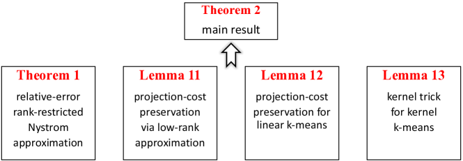
Figure 9: The structure of the proof of Theorem 2.

We use the notation of orthogonal projection matrix throughout this section. A matrix ${\bf M}\in{\mathbb{R}}^{n\times n}$ is an orthogonal projection matrix if and only if there exists a matrix ${\bf Q}$ with orthonormal columns such that ${\bf M}={\bf Q}{\bf Q}^{T}$. It follows that ${\bf M}^{T}={\bf M}$, ${\bf M}{\bf M}={\bf M}$, ${\bf M}\preceq{\bf I}_{n}$ and that ${\bf I}_{n}-{\bf M}$ is also an orthogonal projection matrix.

B.1 Projection-Cost Preservation via Low-Rank Approximation

We first define projection-cost preservation, then show that certain low-rank approximations are projection-cost preserving. Projection-cost preservation was named and systematized by Cohen et al. (2015), but the idea has been used in earlier works (Boutsidis et al., 2010, 2015; Feldman et al., 2013; Liang et al., 2014).

Definition 2 (Rank $k$ Projection-Cost Preservation)

Fix a matrix ${\bf A}\in{\mathbb{R}}^{n\times d}$ and error parameters $\epsilon_{1},\epsilon_{2}>0.$ The matrix ${\bf B}\in{\mathbb{R}}^{n\times d}$ has the rank $k$ projection-cost preserving property with respect to ${\bf A}$ if for any rank $k$ orthogonal projection matrices $\mbox{\boldmath$\Pi$\unboldmath}\in{\mathbb{R}}^{n\times n}$,

$$(1-\epsilon_{1})\big{\|}{\bf A}-\mbox{\boldmath$\Pi$\unboldmath}{\bf A}\big{\|}_{F}^{2}\;\leq\;\big{\|}{\bf B}-\mbox{\boldmath$\Pi$\unboldmath}{\bf B}\big{\|}_{F}^{2}+\alpha\;\leq\;(1+\epsilon_{2})\big{\|}{\bf A}-\mbox{\boldmath$\Pi$\unboldmath}{\bf A}\big{\|}_{F}^{2},$$

for some fixed non-negative $\alpha$ that can depend on ${\bf A}$ and ${\bf B}$ but is independent of $\mbox{\boldmath$\Pi$\unboldmath}.$

The next lemma provides a way to construct a projection-cost preserving sketch of ${\bf A}.$ It states that if a rank-$s$ matrix $\tilde{{\bf A}}_{s}$ in the span of ${\bf A}$ is constructed so that $\tilde{{\bf A}}_{s}\tilde{{\bf A}}_{s}^{T}$ approximates ${\bf A}{\bf A}^{T}$ sufficiently well in terms of the trace norm, then $\tilde{{\bf A}}_{s}$ has the projection-cost preserving property. Observe that this lemma explicitly relates projection-cost preserving sketches to approximate matrix multiplication (Drineas et al., 2006; Mahoney, 2011), where the latter is measures with respect to the trace norm (Gittens and Mahoney, 2016). We provide a proof of Lemma 11 in Appendix D.

Lemma 11 (Projection-Cost Preservation via Low-Rank Approximation)

Fix an error parameter $\epsilon\in(0,1)$. Let ${\bf A}\in{\mathbb{R}}^{n\times d}$ and choose a rank-$s$ matrix $\tilde{{\bf A}}_{s}$ that satisfies the following conditions:

1. there is an orthogonal projection matrix ${\bf M}$ such that $\tilde{\bf A}_{s}\tilde{{\bf A}}_{s}^{T}={\bf A}{\bf M}{\bf A}^{T}$, and

2. $\|{\bf A}{\bf A}^{T}-\tilde{\bf A}_{s}\tilde{{\bf A}}_{s}^{T}\|_{*}\leq(1+\epsilon)\big{\|}{\bf A}{\bf A}^{T}-{\bf A}_{s}{\bf A}_{s}^{T}\big{\|}_{*}$.

Then there exists a fixed $\alpha\geq 0$ such that, for any rank $k$ projection matrices $\mbox{\boldmath$\Pi$\unboldmath}\in{\mathbb{R}}^{n\times n}$,

$$\big{\|}({\bf I}_{n}-\mbox{\boldmath$\Pi$\unboldmath}){\bf A}\big{\|}_{F}^{2}\;\leq\;\big{\|}({\bf I}_{n}-\mbox{\boldmath$\Pi$\unboldmath})\tilde{{\bf A}}_{s}\big{\|}_{F}^{2}+\alpha\;\leq\;\big{(}1+\epsilon+\tfrac{k}{s}\big{)}\big{\|}({\bf I}_{n}-\mbox{\boldmath$\Pi$\unboldmath}){\bf A}\big{\|}_{F}^{2}.$$

B.2 Linear $k$-Means Clustering and Projection-Cost Preservation

Linear $k$-means clustering is formally defined by the optimization problem (1). To relate the linear $k$-means clustering problem to the projection-cost preservation property, we use an equivalent formulation of (1) as an optimization over the set of rank-$k$ projection matrices of the form ${\bf X}{\bf X}^{T},$ where ${\bf X}$ is a cluster indicator matrix. This approach was adopted by Boutsidis et al. (2009, 2010, 2015); Cohen et al. (2015); Ding et al. (2005). Following them, we define the cluster indicator matrix in the following and give an example in Figure 10.

Definition 3 (Cluster Indicator Matrices)

Let $n$ and $k$ be given, and let ${\mathcal{J}}_{1},\ldots,{\mathcal{J}}_{k}$ be a $k$-partition of the set $[n]$. The cluster indicator matrix corresponding to ${\mathcal{J}}_{1},\ldots,{\mathcal{J}}_{k}$ is the $n\times k$ matrix ${\bf X}$ defined by

$$x_{ij} = \left\{\begin{array}[]{cc}\frac{1}{\sqrt{|{\mathcal{J}}_{j}|}}&\textrm{if }\,i\in{\mathcal{J}}_{j};\\ 0&\textrm{otherwise}.\end{array}\right.$$

We take ${\mathcal{X}}_{n,k}$ to be the collection of cluster indicator matrices corresponding to all the $k$-partitions of $[n]$.

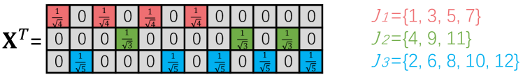
Figure 10: An example of a cluster indicator matrix ${\bf X}\in{\mathcal{X}}_{n,k}$. In this example, $n=12$, $k=3$, and ${\bf X}$ corresponds to the indicated 3-partition ${\mathcal{J}}_{1}$, ${\mathcal{J}}_{2}$, ${\mathcal{J}}_{3}$.

A cluster indicator matrix ${\bf X}$ has exactly one non-zero entry in each row and has orthonormal columns. That is, because of the normalization of the non-zero entries, a cluster indicator matrix ${\bf X}$ is an orthogonal matrix, but one with the additional constraint that there is only one non-zero entry in each row. (Indeed, the insight of Boutsidis et al. (2009, 2010, 2015) was that the rank-constrained optimization over all orthonormal matrices, which provides the usual PCA/SVD-based low-rank approximation, is a relaxation of the optimization over this smaller set of orthonormal matrices.) Among other things, it follows that ${\bf X}{\bf X}^{T}$ is a rank-$k$ projection matrix.

Given this, assume $i\in{\mathcal{J}}_{j}$; it can be verified that the $i$-th row of ${\bf X}{\bf X}^{T}{\bf A}\in{\mathbb{R}}^{n\times d}$ is the centroid of ${\mathcal{J}}_{j}$:

$$({\bf X}{\bf X}^{T}{\bf A})_{i:}\;=\;{\bf x}_{i:}{\bf X}^{T}{\bf A}\;=\;\frac{1}{|{\mathcal{J}}_{j}|}\sum_{l\in{\mathcal{J}}_{j}}{\bf a}_{l:}.$$

Consider the objective function of (1). When ${\bf X}$ is the cluster indicator matrix corresponding to the input $k$-partition, this objective can be rewritten in terms of ${\bf X}{\bf X}^{T}$ as

$$\sum_{j=1}^{k}\sum_{i\in{\mathcal{J}}_{j}}\bigg{\|}{\bf a}_{i:}\,-\,\frac{1}{|{\mathcal{J}}_{j}|}\sum_{l\in{\mathcal{J}}_{j}}{\bf a}_{l:}\bigg{\|}_{2}^{2}\;=\;\sum_{j=1}^{k}\sum_{i\in{\mathcal{J}}_{j}}\big{\|}{\bf a}_{i:}-({\bf X}{\bf X}^{T}{\bf A})_{i:}\big{\|}_{2}^{2}$$

$$=\;\sum_{i=1}^{n}\big{\|}{\bf a}_{i:}-({\bf X}{\bf X}^{T}{\bf A})_{i:}\big{\|}_{2}^{2}\;=\;\big{\|}{\bf A}-{\bf X}{\bf X}^{T}{\bf A}\big{\|}_{F}^{2}.$$

Therefore, the linear $k$-means clustering problem (1) is equivalent to the optimization problem

$$\mathop{\rm argmin}_{{\bf X}\in{\mathcal{X}}_{n,k}}\frac{1}{n}\big{\|}{\bf A}-{\bf X}{\bf X}^{T}{\bf A}\big{\|}_{F}^{2}.$$ (17)

In the remainder of this section, we use this equivalence between $k$-partitionings of $[n]$ and cluster indicator matrices without comment; e.g., we refer to the outputs of linear $k$-means clustering algorithms as cluster indicator matrices. Because the linear $k$-means clustering problem (17) is NP-hard, in practice it is solved by variants of Lloyd’s algorithm.

Definition 4 defines an appropriate notion of approximation for linear $k$-means clustering algorithms. Definition 4 is an equivalent statement of Definition 1.

Definition 4 ($\gamma$-Approximate Algorithms)

We call an algorithm ${\mathcal{A}}_{\gamma}$ ($\gamma\geq 1$) a $\gamma$-approximate linear $k$-means algorithm if it produces a cluster indicator matrix $\tilde{\bf X}$ such that

$$\big{\|}{\bf A}-\tilde{\bf X}\tilde{\bf X}^{T}{\bf A}\big{\|}_{F}^{2}\;\leq\;\gamma\cdot\min_{{\bf X}\in{\mathcal{X}}_{n,k}}\big{\|}{\bf A}-{\bf X}{\bf X}^{T}{\bf A}\big{\|}_{F}^{2}$$

for any conformal matrix ${\bf A}$.

Given this, we now state Lemma 12, which relates projection-cost preservation to linear $k$-means clustering. Let ${\bf A}\in{\mathbb{R}}^{n\times d}$ be the input matrix and ${\bf B}\in{\mathbb{R}}^{n\times s}$ be a smaller matrix ($s<d$) satisfying the projection-cost preservation property. The projection-cost preserving property ensures that the $k$-partition obtained by applying linear $k$-means clustering to the rows of ${\bf B}$, instead of ${\bf A}$, is a good $k$-partition for the rows of ${\bf A}.$ This lemma was established by Cohen et al. (2015). To make this paper self-contained, we provide a proof of Lemma 12 in Appendix E.

Lemma 12 (Projection-Cost Preservation for Linear $k$-Means)

Fix ${\bf A}\in{\mathbb{R}}^{n\times d}$ and assume ${\bf B}\in{\mathbb{R}}^{n\times s}$ satisfies the rank $k$ projection-cost preservation property in Definition 2 with probability at least $1-\delta$. Let the error parameters $\epsilon_{1},\epsilon_{2}\in(0,1)$ be as in Definition 2. If $\tilde{\bf X}_{\bf B}$ is the result of applying a $\gamma$-approximate linear $k$-means clustering algorithm to the rows of ${\bf B},$ then with probability at least $1-2\delta$,

$$\big{\|}{\bf A}-\tilde{\bf X}_{\bf B}\tilde{\bf X}_{\bf B}^{T}{\bf A}\big{\|}_{F}^{2}\;\leq\;\gamma\cdot\tfrac{1+\epsilon_{2}}{1-\epsilon_{1}}\cdot\min_{{\bf X}\in{\mathcal{X}}_{n,k}}\big{\|}{\bf A}-{\bf X}{\bf X}^{T}{\bf A}\big{\|}_{F}^{2}.$$

B.3 Kernel $k$-Means Clustering

Given input vectors ${\bf a}_{1},\ldots,{\bf a}_{n}$, the kernel $k$-means clustering algorithm applies linear $k$-means clustering to feature vectors $\mbox{\boldmath$\phi$\unboldmath}({\bf a}_{1}),\ldots,\mbox{\boldmath$\phi$\unboldmath}({\bf a}_{n})$. For convenience, we let $\mbox{\boldmath$\phi$\unboldmath}({\bf a}_{1})^{T},\ldots,\mbox{\boldmath$\phi$\unboldmath}({\bf a}_{n})^{T}$ constitute the rows of the matrix $\Phi$. Lemma 13 argues that all the information in $\Phi$ relevant to the kernel $k$-means clustering problem is present in the kernel matrix ${\bf K}=\mbox{\boldmath$\Phi$\unboldmath}\mbox{\boldmath$\Phi$\unboldmath}^{T}.$ Variants of this lemma are well-known (Schölkopf and Smola, 2002).

Lemma 13 (Kernel Trick for Kernel $k$-Means)

Let $\Phi$ be a matrix with $n$ rows and let ${\bf K}=\mbox{\boldmath$\Phi$\unboldmath}\mbox{\boldmath$\Phi$\unboldmath}^{T}\in{\mathbb{R}}^{n\times n}$. Let ${\bf K}={\bf V}\mbox{\boldmath$\Lambda$\unboldmath}{\bf V}^{T}$ be the EVD of ${\bf K}$. Then for any matrix ${\bf X}$ with orthonormal columns,

$$\big{\|}\mbox{\boldmath$\Phi$\unboldmath}-{\bf X}{\bf X}^{T}\mbox{\boldmath$\Phi$\unboldmath}\big{\|}_{F}^{2} = \big{\|}({\bf V}\mbox{\boldmath$\Lambda$\unboldmath}^{1/2})-{\bf X}{\bf X}^{T}({\bf V}\mbox{\boldmath$\Lambda$\unboldmath}^{1/2})\big{\|}_{F}^{2}.$$

Proof  Because ${\bf X}$ has orthonormal columns, ${\bf X}{\bf X}^{T}$ is an orthogonal projection matrix, and $({\bf I}_{n}-{\bf X}{\bf X}^{T})$ is the orthogonal projection onto the complementary space. It follows that, as claimed,

$$\big{\|}\mbox{\boldmath$\Phi$\unboldmath}-{\bf X}{\bf X}^{T}\mbox{\boldmath$\Phi$\unboldmath}\big{\|}_{F}^{2}\;=\;\mathrm{tr}\Big{(}\mbox{\boldmath$\Phi$\unboldmath}^{T}({\bf I}_{n}-{\bf X}{\bf X}^{T})\mbox{\boldmath$\Phi$\unboldmath}\Big{)}\;=\;\mathrm{tr}\Big{(}({\bf I}_{n}-{\bf X}{\bf X}^{T}){\bf K}\Big{)}$$

$$=\;\mathrm{tr}\Big{(}({\bf I}_{n}-{\bf X}{\bf X}^{T}){\bf V}\mbox{\boldmath$\Lambda$\unboldmath}^{1/2}\mbox{\boldmath$\Lambda$\unboldmath}^{1/2}{\bf V}({\bf I}_{n}-{\bf X}{\bf X}^{T})\Big{)}\;=\;\big{\|}({\bf V}\mbox{\boldmath$\Lambda$\unboldmath}^{1/2})-{\bf X}{\bf X}^{T}({\bf V}\mbox{\boldmath$\Lambda$\unboldmath}^{1/2})\big{\|}_{F}^{2}.$$

The equalities are justified by, respectively, the definition of the squared Frobenius norm and the idempotence of projections; the cyclicity of the trace and the fact that ${\bf K}=\mbox{\boldmath$\Phi$\unboldmath}\mbox{\boldmath$\Phi$\unboldmath}^{T}$; the cylicity of the trace and the EVD of $\mathbf{K}$; and the definition of the squared Frobenius norm.  

B.4 Completing the Proof of Theorem 2

To complete the proof of Theorem 2, we first establish Lemma 14, and then use it to prove Theorem 15, which is equivalent to Theorem 2. Let $\Phi$ be a matrix with $n$ rows, and ${\bf K}=\mbox{\boldmath$\Phi$\unboldmath}\mbox{\boldmath$\Phi$\unboldmath}^{T}\in{\mathbb{R}}^{n\times n}$ be the corresponding kernel matrix.

Lemma 14

Assume that ${\bf B}\in{\mathbb{R}}^{n\times s}$ satisfies

$$\mathrm{tr}\big{(}{\bf K}-{\bf B}{\bf B}^{T}\big{)}\;\leq\;(1+\epsilon)\big{\|}{\bf K}-{\bf K}_{s}\big{\|}_{*}$$ (18)

and that there is an orthogonal projection matrix ${\bf M}$ such that

$${\bf B}{\bf B}^{T}\;=\;{\bf K}^{1/2}{\bf M}{\bf K}^{1/2}.$$ (19)

Use the rows of ${\bf B}$ as input to a $\gamma$-approximation algorithm (see Definition 4) and let $\tilde{{\bf X}}_{\bf B}$ be the output cluster indicator matrix (see Definition 3), then

$$\big{\|}\mbox{\boldmath$\Phi$\unboldmath}-\tilde{\bf X}_{\bf B}\tilde{\bf X}_{\bf B}^{T}\mbox{\boldmath$\Phi$\unboldmath}\big{\|}_{F}^{2}\;\leq\;\gamma\big{(}1+\epsilon+\tfrac{k}{s}\big{)}\cdot\min_{{\bf X}\in{\mathcal{X}}_{n,k}}\big{\|}\mbox{\boldmath$\Phi$\unboldmath}-{\bf X}{\bf X}^{T}\mbox{\boldmath$\Phi$\unboldmath}\big{\|}_{F}^{2}.$$

Proof  Because assumptions (18) and (19) are satisfied, Lemma 11 ensures that ${\bf B}$ is a rank $k$ projection-cost preserving sketch of ${\bf K}$. That is, there exists a constant $\alpha\geq 0$ independent of $\Pi$ such that

$$\big{\|}({\bf I}_{n}-\mbox{\boldmath$\Pi$\unboldmath}){\bf K}^{1/2}\big{\|}_{F}^{2}\;\leq\;\big{\|}({\bf I}_{n}-\mbox{\boldmath$\Pi$\unboldmath}){\bf B}\big{\|}_{F}^{2}+\alpha\;\leq\;\big{(}1+\epsilon+\tfrac{k}{s}\big{)}\big{\|}({\bf I}_{n}-\mbox{\boldmath$\Pi$\unboldmath}){\bf K}^{1/2}\big{\|}_{F}^{2}$$

holds for any rank-$k$ orthogonal projection matrix $\Pi$. It follows by Lemma 12 that $\tilde{\bf X}_{\bf B}$ gives an almost optimal linear $k$-means clustering over the rows of ${\bf K}^{1/2}$:

$$\big{\|}{\bf K}^{1/2}-\tilde{\bf X}_{\bf B}\tilde{\bf X}_{\bf B}^{T}{\bf K}^{1/2}\big{\|}_{F}^{2}\;\leq\;\gamma\big{(}1+\epsilon+\tfrac{k}{s}\big{)}\cdot\min_{{\bf X}\in{\mathcal{X}}_{n,k}}\big{\|}{\bf K}^{1/2}-{\bf X}{\bf X}^{T}{\bf K}^{1/2}\big{\|}_{F}^{2}.$$

Finally, Lemma 13 states that clustering the rows of ${\bf K}^{1/2}$ is equivalent to clustering the rows of $\Phi$, so we reach the desired conclusion that

$$\big{\|}\mbox{\boldmath$\Phi$\unboldmath}-\tilde{\bf X}_{\bf B}\tilde{\bf X}_{\bf B}^{T}\mbox{\boldmath$\Phi$\unboldmath}\big{\|}_{F}^{2}\;\leq\;\gamma\big{(}1+\epsilon+\tfrac{k}{s}\big{)}\cdot\min_{{\bf X}\in{\mathcal{X}}_{n,k}}\big{\|}\mbox{\boldmath$\Phi$\unboldmath}-{\bf X}{\bf X}^{T}\mbox{\boldmath$\Phi$\unboldmath}\big{\|}_{F}^{2}.$$

 

Finally, we state and prove Theorem 15. Theorem 15 shows that approximate kernel $k$-means clustering using the Nyström method exhibits a $1+\epsilon+\tfrac{k}{s}$ approximation ratio. Observe that Theorem 15 is equivalent to Theorem 2, and thus establishing it also establishes Theorem 2. Recall the Nyström approximation is ${\bf K}\approx{\bf C}{\bf W}^{\dagger}{\bf C}^{T}$, where ${\bf C}={\bf K}{\bf P}$, ${\bf W}={\bf P}^{T}{\bf K}{\bf P}$, and ${\bf P}$ is a sketching matrix.

Theorem 15

Choose a sketching sketching matrix ${\bf P}\in{\mathbb{R}}^{n\times c}$ and sketch size $c$ consistent with Table 2. Let ${\bf B}\in{\mathbb{R}}^{n\times s}$ be any matrix satisfying ${\bf B}{\bf B}^{T}=({\bf C}{\bf W}^{\dagger}{\bf C}^{T})_{s}$. Let the cluster indicator matrix ${\bf X}_{\bf B}$ be the output of any $\gamma$-approximate $k$-means clustering algorithm applied to the rows of ${\bf B}$. With probability at least $0.9$,

$$\big{\|}\mbox{\boldmath$\Phi$\unboldmath}-{\bf X}_{\bf B}{\bf X}_{\bf B}^{T}\mbox{\boldmath$\Phi$\unboldmath}\big{\|}_{F}^{2}\;\leq\;\gamma\big{(}1+\epsilon+\tfrac{k}{s}\big{)}\min_{{\bf X}\in{\mathcal{X}}_{n,k}}\big{\|}\mbox{\boldmath$\Phi$\unboldmath}-{\bf X}{\bf X}^{T}\mbox{\boldmath$\Phi$\unboldmath}\big{\|}_{F}^{2}.$$

Proof  Theorem 1 shows that (18) holds with probability at least $0.9$. Theorem 1 also shows that ${\bf B}{\bf B}^{T}={\bf K}^{1/2}{\bf Q}{\bf Q}^{T}{\bf K}^{1/2}$ where ${\bf Q}$ is a $n\times s$ matrix with orthonormal columns, so (19) holds surely. The theorem now follows from Lemma 14.  

C Proof of Theorem 4

Section C.1 analyzes rank-restricted Nystöm with power method. Section C.2 completes the proof of Theorem 4. Here we re-state the algorithm of Theorem 4: first, set any $c\geq s$ and draw a Gaussian projection matrix ${\bf P}\in{\mathbb{R}}^{n\times c}$; second, run the power iteration ${\bf P}\longleftarrow{\bf K}{\bf P}$ for $t$ times; third, orthogonalize ${\bf P}\in{\mathbb{R}}^{n\times c}$ to obtain ${\bf U}\in{\mathbb{R}}^{n\times c}$; fourth, compute ${\bf C}={\bf K}{\bf U}$ and ${\bf W}={\bf U}^{T}{\bf K}{\bf U}$; last, find any ${\bf B}\in{\mathbb{R}}^{n\times s}$ satisfying ${\bf B}{\bf B}^{T}=({\bf C}{\bf W}^{\dagger}{\bf C}^{T})_{s}$.

C.1 Rank-Restricted Nyström with Power Method

Theorem 16 analyzes the rank-restricted Nyström with power method. The theorem will be used to prove Theorem 4.

Theorem 16

Let ${\bf K}\in{\mathbb{R}}^{n\times n}$ be an SPSD matrix, $s$ be the target rank, $c$ ($\geq s$) be arbitrary, and $\epsilon\in(0,1)$ be an approximation parameter. Let ${\bf C}\in{\mathbb{R}}^{n\times c}$ and ${\bf W}\in{\mathbb{R}}^{c\times c}$ be computed by the above algorithm with $t={\mathcal{O}}(\frac{\log(n/\epsilon)}{\log(\sigma_{s}/\sigma_{s+1})})$ power iterations, where $\sigma_{i}$ is the $i$-th singular value of ${\bf K}$. If $c=s+{\mathcal{O}}(\log\frac{1}{\delta})$, then

$$\big{\|}{\bf K}-({\bf C}{\bf W}^{\dagger}{\bf C}^{T})_{s}\big{\|}_{*} \leq (1+\epsilon)\,\big{\|}{\bf K}-{\bf K}_{s}\big{\|}_{*}$$

with probability at least $1-\delta$. If $c=s$, then this bound holds with a constant probability (that depends on $s$).

Proof  Let ${\bf V}_{-s}\in{\mathbb{R}}^{n\times(n-s)}$ be the orthogonal complement of ${\bf V}_{s}$. Let ${\bf P}$ be an $n\times c$ standard Gaussian matrix. Then ${\bf V}_{-s}^{T}{\bf P}$ is $(n-s)\times c$ standard Gaussian matrix, and ${\bf V}_{s}^{T}{\bf P}$ is $s\times c$ standard Gaussian matrix.

It is well known that the largest singular value of an $(n-s)\times c$ standard Gaussian matrix is at most $\sqrt{n-s}+\sqrt{c}+\zeta$ with probability $1-\exp(-\zeta^{2}/2)$. See (Vershynin, 2010).

Consider $c>s$. The least singular value of an $s\times c$ standard Gaussian matrix is at least $\sqrt{c}-\sqrt{s}-\zeta$ with probability $1-\exp(-\zeta^{2}/2)$. Combining the above results, we have that

$$\frac{\sigma_{1}^{2}({\bf V}_{-s}^{T}{\bf P})}{\sigma_{s}^{2}({\bf V}_{s}^{T}{\bf P})}\;\leq\;\frac{\sqrt{n-s}+\sqrt{c}+\sqrt{2\log(1/\delta)}}{\sqrt{c}-\sqrt{s}-\sqrt{2\log(1/\delta)}}$$

holds with probability $1-2\delta$.

Consider $c=s$. Rudelson and Vershynin (2008); Tao and Vu (2010) showed that the least singular value of an $s\times s$ standard Gaussian matrix ${\bf G}$ satisfy

$${\mathbb{P}}\big{\{}\sigma_{s}({\bf G})\leq\tfrac{\delta_{1}}{\sqrt{s}}\big{\}}\;=\;\delta_{1}+{\mathcal{O}}(s^{-\tau}),$$

where $\tau>0$ is a constant. It follows that

$$\frac{\sigma_{1}^{2}({\bf V}_{-s}^{T}{\bf P})}{\sigma_{s}^{2}({\bf V}_{s}^{T}{\bf P})}\;\leq\;\frac{\sqrt{n-s}+\sqrt{s}+\sqrt{2\log(1/\delta_{2})}}{\delta_{1}/\sqrt{s}}$$

holds with probability $1-\delta_{1}-\delta_{2}-{\mathcal{O}}(s^{-\tau})$.

For either $c>s$ or $c=s$, it follows from Lemma 17, which will be proved subsequently, that

$$\big{\|}{\bf K}-({\bf C}{\bf W}^{\dagger}{\bf C}^{T})_{s}\big{\|}_{*} \leq \big{\|}{\bf K}-{\bf K}_{s}\big{\|}_{*}+\tfrac{\sigma_{1}^{2}({\bf V}_{-s}^{T}{\bf P})}{\sigma_{s}^{2}({\bf V}_{s}^{T}{\bf P})}\,\Big{(}\tfrac{\sigma_{s+1}({\bf K})}{\sigma_{s}({\bf K})}\Big{)}^{2t}\,\big{\|}{\bf K}-{\bf K}_{s}\big{\|}_{*}$$

$$\leq \big{\|}{\bf K}-{\bf K}_{s}\big{\|}_{*}+{\mathcal{O}}\big{(}ns\big{)}\,\Big{(}\tfrac{\sigma_{s+1}({\bf K})}{\sigma_{s}({\bf K})}\Big{)}^{2t}\,\big{\|}{\bf K}-{\bf K}_{s}\big{\|}_{*}$$

holds with constant probability, by which the theorem follows.  

Lemma 17

Let ${\bf K}\in{\mathbb{R}}^{n\times n}$ be any fixed SPSD matrix, $s$ and $t$ be any positive integer, and ${\bf V}_{s}\in{\mathbb{R}}^{n\times s}$ be the top $s$ singular vectors of ${\bf K}$. Let ${\bf P}\in{\mathbb{R}}^{n\times c}$ satisfy that ${\bf P}^{T}{\bf V}_{s}\in{\mathbb{R}}^{c\times s}$ has full column rank. Let ${\bf U}\in{\mathbb{R}}^{n\times c}$ be the orthonormal bases of ${\bf K}^{t}{\bf P}$. Let ${\bf C}={\bf K}{\bf U}$ and ${\bf W}={\bf U}^{T}{\bf K}{\bf U}$. Then

$$\big{\|}{\bf K}-({\bf C}{\bf W}^{\dagger}{\bf C}^{T})_{s}\big{\|}_{*}\;\leq\;\big{\|}{\bf K}-{\bf K}_{s}\big{\|}_{*}+\Big{(}\tfrac{\sigma_{s+1}({\bf K})}{\sigma_{s}({\bf K})}\Big{)}^{2t}\,\tfrac{\sigma_{1}^{2}({\bf V}_{-s}^{T}{\bf P})}{\sigma_{s}^{2}({\bf V}_{s}^{T}{\bf P})}\,\big{\|}{\bf K}-{\bf K}_{s}\big{\|}_{*}.$$

Here ${\bf V}_{-s}\in{\mathbb{R}}^{n\times(n-s)}$ is the orthogonal complement of ${\bf V}_{s}$.

Proof  It follows from Lemma 8 that

$$\big{\|}{\bf K}-\big{(}{\bf C}{\bf W}^{\dagger}{\bf C}^{T}\big{)}_{s}\big{\|}_{*} = \min_{\mathrm{rank}({\bf Z})\leq s}\big{\|}{\bf K}^{1/2}-({\bf K}^{1/2}{\bf U}){\bf Z}\big{\|}_{F}^{2}$$

$$= \min_{\mathrm{rank}({\bf Z})\leq s}\big{\|}{\bf A}-({\bf A}{\bf U}){\bf Z}\big{\|}_{F}^{2}$$

where we let ${\bf A}={\bf K}^{1/2}$. By definition, ${\bf U}$ contains the orthonormal bases of ${\bf K}^{t}{\bf P}={\bf A}^{2t}{\bf P}$, and thus there exists an $s\times s$ non-singular matrix ${\bf R}$ such that ${\bf A}^{2t}{\bf P}={\bf U}{\bf R}$. It follows that

$$\big{\|}{\bf K}-\big{(}{\bf C}{\bf W}^{\dagger}{\bf C}^{T}\big{)}_{s}\big{\|}_{*} = \min_{\mathrm{rank}({\bf Z})\leq s}\big{\|}{\bf A}-({\bf A}{\bf A}^{2t}{\bf P}{\bf R}^{-1}){\bf Z}\big{\|}_{F}^{2}$$

$$= \min_{\mathrm{rank}({\bf Y})\leq s}\big{\|}{\bf A}-({\bf A}^{2t+1}{\bf P}){\bf Y}\big{\|}_{F}^{2},$$

where the latter equality follows from that the column spaces of ${\bf A}^{2t+1}{\bf P}$ and ${\bf A}^{2t+1}{\bf P}{\bf R}^{-1}$ are the same. It follows from Lemma 7 that

$$\big{\|}{\bf K}-\big{(}{\bf C}{\bf W}^{\dagger}{\bf C}^{T}\big{)}_{s}\big{\|}_{*}\;=\;\min_{\mathrm{rank}({\bf Y})\leq s}\big{\|}{\bf A}-({\bf A}^{2t+1}{\bf P}){\bf Y}\big{\|}_{F}^{2}$$

$$\leq\;\big{\|}{\bf A}-{\bf A}_{s}\big{\|}_{F}^{2}+\Big{(}\tfrac{\sigma_{s+1}^{2}({\bf A})}{\sigma_{s}^{2}({\bf A})}\Big{)}^{2t}\,\Big{\|}({\bf A}-{\bf A}_{s}){\bf P}({\bf V}_{s}^{T}{\bf P})^{\dagger}\Big{\|}_{F}^{2}$$

$$\leq\;\big{\|}{\bf A}-{\bf A}_{s}\big{\|}_{F}^{2}+\Big{(}\tfrac{\sigma_{s+1}^{2}({\bf A})}{\sigma_{s}^{2}({\bf A})}\Big{)}^{2t}\,\big{\|}{\bf A}-{\bf A}_{s}\big{\|}_{F}^{2}\big{\|}{\bf V}_{-s}^{T}{\bf P}\big{\|}_{2}^{2}\big{\|}({\bf V}_{s}^{T}{\bf P})^{\dagger}\big{\|}_{2}^{2},$$

where we define ${\bf V}_{-s}\in{\mathbb{R}}^{n\times(n-s)}$ as the orthogonal complement of ${\bf V}_{s}$. By our definition ${\bf A}={\bf K}^{1/2}$, it follows that

$$\big{\|}{\bf K}-\big{(}{\bf C}{\bf W}^{\dagger}{\bf C}^{T}\big{)}_{s}\big{\|}_{*}$$

$$\leq\;\big{\|}({\bf K}-{\bf K}_{s})^{1/2}\big{\|}_{F}^{2}+\Big{(}\tfrac{\sigma_{s+1}({\bf K})}{\sigma_{s}({\bf K})}\Big{)}^{2t}\,\tfrac{\sigma_{1}^{2}({\bf V}_{-s}^{T}{\bf P})}{\sigma_{s}^{2}({\bf V}_{s}^{T}{\bf P})}\,\big{\|}({\bf K}-{\bf K}_{s})^{1/2}\big{\|}_{F}^{2}$$

$$=\;\big{\|}{\bf K}-{\bf K}_{s}\big{\|}_{*}+\Big{(}\tfrac{\sigma_{s+1}({\bf K})}{\sigma_{s}({\bf K})}\Big{)}^{2t}\,\tfrac{\sigma_{1}^{2}({\bf V}_{-s}^{T}{\bf P})}{\sigma_{s}^{2}({\bf V}_{s}^{T}{\bf P})}\,\big{\|}{\bf K}-{\bf K}_{s}\big{\|}_{*},$$

by which the lemma follows.  

C.2 Completing the Proof of Theorem 4

Finally, we state and prove Theorem 18. Observe that Theorem 18 is equivalent to Theorem 4, and thus establishing it also establishes Theorem 4.

Theorem 18

Let $c$, $t$, and ${\bf B}\in{\mathbb{R}}^{n\times s}$ be defined in the begining of this section. Set $t={\mathcal{O}}(\frac{\log(n/\epsilon)}{\log(\sigma_{s}/\sigma_{s+1})})$. Let the cluster indicator matrix ${\bf X}_{\bf B}$ be the output of any $\gamma$-approximate $k$-means clustering algorithm applied to the rows of ${\bf B}$. If $c=s+{\mathcal{O}}(\log\frac{1}{\delta})$, then

$$\big{\|}\mbox{\boldmath$\Phi$\unboldmath}-{\bf X}_{\bf B}{\bf X}_{\bf B}^{T}\mbox{\boldmath$\Phi$\unboldmath}\big{\|}_{F}^{2}\;\leq\;\gamma\big{(}1+\epsilon+\tfrac{k}{s}\big{)}\min_{{\bf X}\in{\mathcal{X}}_{n,k}}\big{\|}\mbox{\boldmath$\Phi$\unboldmath}-{\bf X}{\bf X}^{T}\mbox{\boldmath$\Phi$\unboldmath}\big{\|}_{F}^{2}$$

holds with probability at least $1-\delta$. If $c=s$, then the above inequality holds with probability $0.9-{\mathcal{O}}(s^{-\tau})$, where $\tau$ is a constant.

Proof  Since ${\bf B}{\bf B}^{T}=({\bf C}{\bf W}^{\dagger}{\bf C}^{T})_{s}$ by definition, Theorem 16 ensures that (18) holds with some constant probability. Theorem 1 shows that ${\bf B}{\bf B}^{T}={\bf K}^{1/2}{\bf Q}{\bf Q}^{T}{\bf K}^{1/2}$ where ${\bf Q}$ is a $n\times s$ matrix with orthonormal columns, so (19) holds surely. The theorem now follows from Lemma 14.  

D Proof of Lemma 11

To prove Lemma 11, we first establish a key lemma, Lemma 19. This lemma will make use of the following two assumptions.

Assumption 1

Assume that $\tilde{{\bf A}}_{s}$ satisfies $\mathrm{tr}\big{(}{\bf A}{\bf A}^{T}-\tilde{\bf A}_{s}\tilde{{\bf A}}_{s}^{T}\big{)}\leq(1+\epsilon)\big{\|}{\bf A}{\bf A}^{T}-{\bf A}_{s}{\bf A}_{s}^{T}\big{\|}_{*}$.

Assumption 2

Assume there exists such an orthogonal projection matrix ${\bf M}$ that $\tilde{\bf A}_{s}\tilde{{\bf A}}_{s}^{T}={\bf A}{\bf M}{\bf A}^{T}$.

Lemma 19

Let ${\bf A}\in{\mathbb{R}}^{n\times d}$ be any fixed matrix. Fix an error parameter $\epsilon\in(0,1)$. Let the rank $s$ matrix $\tilde{{\bf A}}_{s}$ satisfy Assumptions 1 and 2. Then for any rank $k$ orthogonal projection matrix $\mbox{\boldmath$\Pi$\unboldmath}\in{\mathbb{R}}^{n\times n}$,

$$\mathrm{tr}\Big{(}\mbox{\boldmath$\Pi$\unboldmath}\big{(}{\bf A}{\bf A}^{T}-\tilde{\bf A}_{s}\tilde{\bf A}_{s}^{T}\big{)}\mbox{\boldmath$\Pi$\unboldmath}\Big{)}\;\leq\;\big{(}\epsilon+\tfrac{k}{s}\big{)}\big{\|}{\bf A}-\mbox{\boldmath$\Pi$\unboldmath}{\bf A}\big{\|}_{F}^{2}.$$

Proof  It holds that

$$\mathrm{tr}\Big{(}({\bf I}_{n}-\mbox{\boldmath$\Pi$\unboldmath})\big{(}{\bf A}{\bf A}^{T}-\tilde{\bf A}_{s}\tilde{\bf A}_{s}^{T}\big{)}\Big{)}$$

$$=\;\mathrm{tr}\Big{(}\big{(}{\bf A}{\bf A}^{T}-\tilde{\bf A}_{s}\tilde{\bf A}_{s}^{T}\big{)}-\mbox{\boldmath$\Pi$\unboldmath}\big{(}{\bf A}{\bf A}^{T}-\tilde{\bf A}_{s}\tilde{\bf A}_{s}^{T}\big{)}\Big{)}$$

$$=\;\mathrm{tr}\big{(}{\bf A}{\bf A}^{T}-\tilde{\bf A}_{s}\tilde{\bf A}_{s}^{T}\big{)}-\mathrm{tr}\big{(}\mbox{\boldmath$\Pi$\unboldmath}\big{(}{\bf A}{\bf A}^{T}-\tilde{\bf A}_{s}\tilde{\bf A}_{s}^{T}\big{)}\mbox{\boldmath$\Pi$\unboldmath}\big{)}$$

$$\leq\;(1+\epsilon)\big{\|}{\bf A}{\bf A}^{T}-{\bf A}_{s}{\bf A}_{s}^{T}\big{\|}_{*}-\mathrm{tr}\big{(}\mbox{\boldmath$\Pi$\unboldmath}\big{(}{\bf A}{\bf A}^{T}-\tilde{\bf A}_{s}\tilde{\bf A}_{s}^{T}\big{)}\mbox{\boldmath$\Pi$\unboldmath}\big{)},$$

where the inequality follows from Assumption 1. It can be equivalently written as

$$\mathrm{tr}\Big{(}\mbox{\boldmath$\Pi$\unboldmath}\big{(}{\bf A}{\bf A}^{T}-\tilde{\bf A}_{s}\tilde{\bf A}_{s}^{T}\big{)}\mbox{\boldmath$\Pi$\unboldmath}\Big{)}$$

$$\leq\;(1+\epsilon)\big{\|}{\bf A}{\bf A}^{T}-{\bf A}_{s}{\bf A}_{s}^{T}\big{\|}_{*}-\mathrm{tr}\Big{(}({\bf I}_{n}-\mbox{\boldmath$\Pi$\unboldmath})\big{(}{\bf A}{\bf A}^{T}-\tilde{\bf A}_{s}\tilde{\bf A}_{s}^{T}\big{)}({\bf I}_{n}-\mbox{\boldmath$\Pi$\unboldmath})\Big{)}.$$

Let ${\bf M}$ be an orthogonal projection matrix defined in Assumption 2; by this assumption, it holds that $\tilde{\bf A}_{s}\tilde{\bf A}_{s}^{T}={\bf A}{\bf M}{\bf A}^{T}$ and $\mathrm{rank}({\bf M}{\bf A})=s$. It follows that

$$\mathrm{tr}\Big{(}({\bf I}_{n}-\mbox{\boldmath$\Pi$\unboldmath})\big{(}{\bf A}{\bf A}^{T}-\tilde{\bf A}_{s}\tilde{\bf A}_{s}^{T}\big{)}({\bf I}_{n}-\mbox{\boldmath$\Pi$\unboldmath})\Big{)}\;=\;\mathrm{tr}\Big{(}({\bf I}_{n}-\mbox{\boldmath$\Pi$\unboldmath}){\bf A}({\bf I}-{\bf M}){\bf A}^{T}({\bf I}_{n}-\mbox{\boldmath$\Pi$\unboldmath})\Big{)}$$

$$=\;\big{\|}({\bf I}_{n}-\mbox{\boldmath$\Pi$\unboldmath}){\bf A}({\bf I}-{\bf M})\big{\|}_{F}^{2}\;=\;\Big{\|}{\bf A}-\underbrace{\mbox{\boldmath$\Pi$\unboldmath}{\bf A}}_{\textrm{rank }k}-\underbrace{({\bf I}_{n}-\mbox{\boldmath$\Pi$\unboldmath}){\bf A}{\bf M}}_{\textrm{rank }s}\Big{\|}_{F}^{2}$$

$$\geq\;\min_{\mathrm{rank}({\bf Y})\leq s+k}\big{\|}{\bf A}-{\bf Y}\big{\|}_{F}^{2}\;=\;\big{\|}{\bf A}-{\bf A}_{s+k}\big{\|}_{F}^{2},$$

where the inequality follows from that matrix rank is subadditive function. It follows that

$$\mathrm{tr}\Big{(}\mbox{\boldmath$\Pi$\unboldmath}\big{(}{\bf A}{\bf A}^{T}-\tilde{\bf A}_{s}\tilde{\bf A}_{s}^{T}\big{)}\mbox{\boldmath$\Pi$\unboldmath}\Big{)}$$

$$\leq\;(1+\epsilon)\big{\|}{\bf A}{\bf A}^{T}-{\bf A}_{s}{\bf A}_{s}^{T}\big{\|}_{*}-\big{\|}{\bf A}-{\bf A}_{s+k}\big{\|}_{F}^{2}$$

$$=\;(1+\epsilon)\big{\|}{\bf A}-{\bf A}_{s}\big{\|}_{F}^{2}-\big{\|}{\bf A}-{\bf A}_{s+k}\big{\|}_{F}^{2}$$

$$=\;\epsilon\big{\|}{\bf A}-{\bf A}_{s}\big{\|}_{F}^{2}+\sum_{i=s+1}^{n}\sigma_{i}^{2}({\bf A})-\sum_{i=s+k+1}^{n}\sigma_{i}^{2}({\bf A})$$

$$=\;\epsilon\big{\|}{\bf A}-{\bf A}_{s}\big{\|}_{F}^{2}+\sum_{i=s+1}^{s+k}\sigma_{i}^{2}({\bf A})$$

$$\leq\;\epsilon\big{\|}{\bf A}-{\bf A}_{s}\big{\|}_{F}^{2}+\frac{k}{s}\sum_{i=k+1}^{s+k}\sigma_{i}^{2}({\bf A}),$$

where the last inequality follows by the decrease of the singular values. Finally, we obtain that

$$\mathrm{tr}\Big{(}\mbox{\boldmath$\Pi$\unboldmath}\big{(}{\bf A}{\bf A}^{T}-\tilde{\bf A}_{s}\tilde{\bf A}_{s}^{T}\big{)}\mbox{\boldmath$\Pi$\unboldmath}\Big{)}\;\leq\;\epsilon\big{\|}{\bf A}-{\bf A}_{k}\big{\|}_{F}^{2}+\tfrac{k}{s}\big{\|}{\bf A}-{\bf A}_{k}\big{\|}_{F}^{2}\;\leq\;\big{(}\epsilon+\tfrac{k}{s}\big{)}\big{\|}{\bf A}-\mbox{\boldmath$\Pi$\unboldmath}{\bf A}\big{\|}_{F}^{2},$$

by which the lemma follows.  

Given Lemma 19, we now provide the proof of Lemma 11.

Proof  For any orthogonal projection matrix ${\bf M}$, it holds that ${\bf M}={\bf M}{\bf M}$. It follows that

$$\big{\|}({\bf I}_{n}-\mbox{\boldmath$\Pi$\unboldmath}){\bf A}\big{\|}_{F}^{2}-\big{\|}({\bf I}_{n}-\mbox{\boldmath$\Pi$\unboldmath})\tilde{\bf A}_{s}\big{\|}_{F}^{2}\;=\;\mathrm{tr}\big{(}({\bf I}_{n}-\mbox{\boldmath$\Pi$\unboldmath}){\bf A}{\bf A}^{T}\big{)}-\mathrm{tr}\big{(}({\bf I}_{n}-\mbox{\boldmath$\Pi$\unboldmath})\tilde{\bf A}_{s}\tilde{\bf A}_{s}^{T}\big{)}$$

$$=\;\mathrm{tr}\big{(}({\bf I}_{n}-\mbox{\boldmath$\Pi$\unboldmath})({\bf A}{\bf A}^{T}-\tilde{\bf A}_{s}\tilde{\bf A}_{s}^{T})\big{)}\;=\;\mathrm{tr}\big{(}{\bf A}{\bf A}^{T}-\tilde{\bf A}_{s}\tilde{\bf A}_{s}^{T}\big{)}-\mathrm{tr}\big{(}\mbox{\boldmath$\Pi$\unboldmath}({\bf A}{\bf A}^{T}-\tilde{\bf A}_{s}\tilde{\bf A}_{s}^{T})\big{)}$$

$$\;=\;\alpha-\mathrm{tr}\big{(}\mbox{\boldmath$\Pi$\unboldmath}({\bf A}{\bf A}^{T}-\tilde{\bf A}_{s}\tilde{\bf A}_{s}^{T})\big{)},$$

where the last equality follows by letting $\alpha=\mathrm{tr}\big{(}{\bf A}{\bf A}^{T}-\tilde{\bf A}_{s}\tilde{\bf A}_{s}^{T}\big{)}\geq 0$ which is independent of $\Pi$. The above equality can be equivalently written as

$$\big{\|}({\bf I}_{n}-\mbox{\boldmath$\Pi$\unboldmath})\tilde{\bf A}_{s}\big{\|}_{F}^{2}+\alpha = \big{\|}({\bf I}_{n}-\mbox{\boldmath$\Pi$\unboldmath}){\bf A}\big{\|}_{F}^{2}+\mathrm{tr}\big{(}\mbox{\boldmath$\Pi$\unboldmath}({\bf A}{\bf A}^{T}-\tilde{\bf A}_{s}\tilde{\bf A}_{s}^{T})\mbox{\boldmath$\Pi$\unboldmath}\big{)}.$$ (20)

Under Assumption 2 that $\tilde{\bf A}_{s}\tilde{\bf A}_{s}^{T}\preceq{\bf A}{\bf A}^{T}$, it follows from (20) that

$$\big{\|}({\bf I}_{n}-\mbox{\boldmath$\Pi$\unboldmath}){\bf A}\big{\|}_{F}^{2}$$

$$\leq\;\big{\|}({\bf I}_{n}-\mbox{\boldmath$\Pi$\unboldmath})\tilde{\bf A}_{s}\big{\|}_{F}^{2}+\alpha$$

$$=\;\big{\|}({\bf I}_{n}-\mbox{\boldmath$\Pi$\unboldmath}){\bf A}\big{\|}_{F}^{2}+\mathrm{tr}\big{(}\mbox{\boldmath$\Pi$\unboldmath}({\bf A}{\bf A}^{T}-\tilde{\bf A}_{s}\tilde{\bf A}_{s}^{T})\mbox{\boldmath$\Pi$\unboldmath}\big{)}.$$

Under Assumptions 1 and 2, we can apply Lemma 19 to bound the right-hand side:

$$\mathrm{tr}\Big{(}\mbox{\boldmath$\Pi$\unboldmath}\big{(}{\bf A}{\bf A}^{T}-\tilde{\bf A}_{s}\tilde{\bf A}_{s}^{T}\big{)}\mbox{\boldmath$\Pi$\unboldmath}\Big{)}\;\leq\;\big{(}\epsilon+\tfrac{k}{s}\big{)}\big{\|}{\bf A}-\mbox{\boldmath$\Pi$\unboldmath}{\bf A}\big{\|}_{F}^{2},$$

by which the lemma follows.  

E Proof of Lemma 12

Because ${\bf B}$ enjoys the projection-cost preservation property, there exists a constant $\alpha\geq 0$ such that for any rank $k$ orthogonal projection matrices $\mbox{\boldmath$\Pi$\unboldmath}_{1}$ and $\mbox{\boldmath$\Pi$\unboldmath}_{2}$, the two inequalities

$$(1-\epsilon_{1})\big{\|}{\bf A}-\mbox{\boldmath$\Pi$\unboldmath}_{1}{\bf A}\big{\|}_{F}^{2}\;\leq\;\big{\|}{\bf B}-\mbox{\boldmath$\Pi$\unboldmath}_{1}{\bf B}\big{\|}_{F}^{2}+\alpha,$$ (21)

$$\big{\|}{\bf B}-\mbox{\boldmath$\Pi$\unboldmath}_{2}{\bf B}\big{\|}_{F}^{2}+\alpha\;\leq\;(1+\epsilon_{2})\big{\|}{\bf A}-\mbox{\boldmath$\Pi$\unboldmath}_{2}{\bf A}\big{\|}_{F}^{2}$$ (22)

hold simultaneously with probability at least $1-2\delta$. Let $\mbox{\boldmath$\Pi$\unboldmath}_{1}=\tilde{\bf X}_{\bf B}\tilde{\bf X}_{\bf B}^{T}$ and ${\bf X}_{\bf A}^{\star}=\mathop{\rm argmin}_{{\bf X}\in{\mathcal{X}}_{n,k}}\|{\bf A}-{\bf X}{\bf X}^{T}{\bf A}\|_{F}^{2}$. It follows from (21) and the definition of $\gamma$-approximate $k$-means algorithm that

$$(1-\epsilon_{1})\big{\|}{\bf A}-\tilde{\bf X}_{\bf B}\tilde{\bf X}_{\bf B}^{T}{\bf A}\big{\|}_{F}^{2}\;\leq\;\big{\|}{\bf B}-\tilde{\bf X}_{\bf B}\tilde{\bf X}_{\bf B}^{T}{\bf B}\big{\|}_{F}^{2}+\alpha$$

$$\leq\;\gamma\cdot\min_{{\bf X}\in{\mathcal{X}}_{n,k}}\big{\|}{\bf B}-{\bf X}{\bf X}^{T}{\bf B}\big{\|}_{F}^{2}+\alpha\;\leq\;\gamma\big{\|}{\bf B}-{\bf X}_{\bf A}^{\star}{{\bf X}_{\bf A}^{\star}}^{T}{\bf B}\big{\|}_{F}^{2}+\alpha.$$

Let $\mbox{\boldmath$\Pi$\unboldmath}_{2}={\bf X}_{\bf A}^{\star}{{\bf X}_{\bf A}^{\star}}^{T}$. It follows from (22) that

$$\big{\|}{\bf B}-{\bf X}_{\bf A}^{\star}{{\bf X}_{\bf A}^{\star}}^{T}{\bf B}\big{\|}_{F}^{2}+\alpha\;\leq\;(1+\epsilon_{2})\big{\|}{\bf A}-{\bf X}_{\bf A}^{\star}{{\bf X}_{\bf A}^{\star}}^{T}{\bf A}\big{\|}_{F}^{2}.$$

Combining the above results, we have that

$$(1-\epsilon_{1})\big{\|}{\bf A}-\tilde{\bf X}_{\bf B}\tilde{\bf X}_{\bf B}^{T}{\bf A}\big{\|}_{F}^{2}\;\leq\;\gamma\big{\|}{\bf B}-{\bf X}_{\bf A}^{\star}{{\bf X}_{\bf A}^{\star}}^{T}{\bf B}\big{\|}_{F}^{2}+\alpha$$

$$\leq\;\gamma\big{(}\big{\|}{\bf B}-{\bf X}_{\bf A}^{\star}{{\bf X}_{\bf A}^{\star}}^{T}{\bf B}\big{\|}_{F}^{2}+\alpha\big{)}\;\leq\;\gamma(1+\epsilon_{2})\big{\|}{\bf A}-{\bf X}_{\bf A}^{\star}{{\bf X}_{\bf A}^{\star}}^{T}{\bf A}\big{\|}_{F}^{2},$$

where the second inequality follows from that $\gamma\geq 1$ and $\alpha\geq 0$. It follows that

$$\big{\|}{\bf A}-\tilde{\bf X}_{\bf B}\tilde{\bf X}_{\bf B}^{T}{\bf A}\big{\|}_{F}^{2}\;\leq\;\gamma\tfrac{1+\epsilon_{2}}{1-\epsilon_{1}}\big{\|}{\bf A}-{\bf X}_{\bf A}^{\star}{{\bf X}_{\bf A}^{\star}}^{T}{\bf A}\big{\|}_{F}^{2}\;=\;\gamma\tfrac{1+\epsilon_{2}}{1-\epsilon_{1}}\min_{{\bf X}\in{\mathcal{X}}_{n,k}}\big{\|}{\bf A}-{\bf X}{{\bf X}}^{T}{\bf A}\big{\|}_{F}^{2}$$

This concludes our proof.

References

- Alaoui and Mahoney (2015) Ahmed Alaoui and Michael W. Mahoney. Fast Randomized Kernel Ridge Regression with Statistical Guarantees. In Advances in Neural Information Processing Systems (NIPS). 2015.
- Aloise et al. (2009) Daniel Aloise, Amit Deshpande, Pierre Hansen, and Preyas Popat. NP-hardness of Euclidean sum-of-squares clustering. Machine Learning, 75(2):245–248, 2009.
- Arikan (2006) Okan Arikan. Compression of motion capture databases. In ACM Transactions on Graphics (TOG), volume 25, pages 890–897. ACM, 2006.
- Arthur and Vassilvitskii (2007) David Arthur and Sergei Vassilvitskii. k-means++: the advantages of careful seeding. In Annual ACM-SIAM Symposium on Discrete Algorithms, 2007.
- Awasthi et al. (2015) Pranjal Awasthi, Moses Charikar, Ravishankar Krishnaswamy, and Ali Kemal Sinop. The hardness of approximation of Euclidean k-means. arXiv preprint arXiv:1502.03316, 2015.
- Bach (2013) Francis Bach. Sharp analysis of low-rank kernel matrix approximations. In International Conference on Learning Theory (COLT), 2013.
- Berg et al. (2004) Tamara L. Berg, Alexander C. Berg, Jaety Edwards, and David A. Forsyth. Who’s in the picture. Advances in Neural Information Processing Systems (NIPS), 2004.
- Boutsidis et al. (2009) Christos Boutsidis, Petros Drineas, and Michael W. Mahoney. Unsupervised Feature Selection for the k-means Clustering Problem. In Advances in Neural Information Processing Systems (NIPS). 2009.
- Boutsidis et al. (2010) Christos Boutsidis, Anastasios Zouzias, and Petros Drineas. Random projections for -means clustering. In Advances in Neural Information Processing Systems (NIPS), 2010.
- Boutsidis et al. (2014) Christos Boutsidis, Petros Drineas, and Malik Magdon-Ismail. Near-Optimal Column-Based Matrix Reconstruction. SIAM Journal on Computing, 43(2):687–717, 2014.
- Boutsidis et al. (2015) Christos Boutsidis, Anastasios Zouzias, Michael W. Mahoney, and Petros Drineas. Randomized Dimensionality Reduction for -Means Clustering. IEEE Transactions on Information Theory, 61(2):1045–1062, 2015.
- Chandola et al. (2009) Varun Chandola, Arindam Banerjee, and Vipin Kumar. Anomaly detection: A survey. ACM Computing Surveys, 41(3):1–58, 2009.
- Chaturvedi et al. (1997) Anil Chaturvedi, J. Douglas Carroll, Paul E. Green, and John A. Rotondo. A feature-based approach to market segmentation via overlapping k-centroids clustering. Journal of Marketing Research, 34(3):370–377, 1997.
- Cheeger (1969) Jeff Cheeger. A lower bound for the smallest eigenvalue of the Laplacian. In Problems in Analysis, Papers dedicated to Salomon Bochner, pages 195–199. Princeton University Press, 1969.
- Chen (2009) Ke Chen. On coresets for k-median and k-means clustering in metric and Euclidean spaces and their applications. SIAM Journal on Computing, 39(3):923–947, 2009.
- Chen et al. (2011) Wen-Yen Chen, Yangqiu Song, Hongjie Bai, Chih-Jen Lin, and Edward Y. Chang. Parallel Spectral Clustering in Distributed Systems. IEEE Transactions on Pattern Analysis and Machine Intelligence, 33(3):568–586, 2011.
- Chitta et al. (2011) Radha Chitta, Rong Jin, Timothy C. Havens, and Anil K. Jain. Approximate Kernel -means: Solution to Large Scale Kernel Clustering. In ACM SIGKDD International Conference on Knowledge Discovery and Data Mining (KDD), 2011.
- Chitta et al. (2012) Radha Chitta, Rong Jin, and Anil K. Jain. Efficient Kernel Clustering Using Random Fourier Features. In IEEE International Conference on Data Mining (ICDM), 2012.
- Chiu and Demanet (2013) Jiawei Chiu and Laurent Demanet. Sublinear Randomized Algorithms for Skeleton Decompositions. SIAM Journal on Matrix Analysis and Applications, 34(3):1361–1383, 2013.
- Clarkson and Woodruff (2013) Kenneth L. Clarkson and David P. Woodruff. Low rank approximation and regression in input sparsity time. In Annual ACM Symposium on Theory of Computing (STOC), 2013.
- Cohen et al. (2015) Michael B Cohen, Sam Elder, Cameron Musco, Christopher Musco, and Madalina Persu. Dimensionality reduction for k-means clustering and low rank approximation. In Annual ACM Symposium on Theory of Computing (STOC), 2015.
- Cohen et al. (2017) Michael B Cohen, Cameron Musco, and Christopher Musco. Input sparsity time low-rank approximation via ridge leverage score sampling. In Annual ACM-SIAM Symposium on Discrete Algorithms (SODA), 2017.
- Cortes et al. (2010) Corinna Cortes, Mehryar Mohri, and Ameet Talwalkar. On the impact of kernel approximation on learning accuracy. In Conference on Artificial Intelligence and Statistics (AISTATS), 2010.
- Dasgupta and Freund (2009) Sanjoy Dasgupta and Yoav Freund. Random projection trees for vector quantization. IEEE Transactions on Information Theory, 55(7):3229–3242, 2009.
- Dhillon et al. (2004) Inderjit S Dhillon, Yuqiang Guan, and Brian Kulis. Kernel k-means: spectral clustering and normalized cuts. In ACM SIGKDD International Conference on Knowledge Discovery and Data Mining (KDD), 2004.
- Ding et al. (2005) Chris Ding, Xiaofeng He, and Horst D Simon. On the equivalence of nonnegative matrix factorization and spectral clustering. In SIAM International Conference on Data Mining (SDM), 2005.
- Donath and Hoffman (1972) William E Donath and Alan J Hoffman. Algorithms for partitioning graphs and computer logic based on eigenvectors of connection matrices. IBM Technical Disclosure Bulletin, 15(3):938–944, 1972.
- Donath and Hoffman (1973) William E Donath and Alan J Hoffman. Lower bounds for the partitioning of graphs. IBM Journal of Research and Development, 17(5):420–425, 1973.
- Drineas and Mahoney (2005) Petros Drineas and Michael W. Mahoney. On the Nyström method for approximating a Gram matrix for improved kernel-based learning. Journal of Machine Learning Research, 6:2153–2175, 2005.
- Drineas and Mahoney (2016) Petros Drineas and Michael W Mahoney. RandNLA: randomized numerical linear algebra. Communications of the ACM, 59(6):80–90, 2016.
- Drineas et al. (2006) Petros Drineas, Ravi Kannan, and Michael W. Mahoney. Fast Monte Carlo algorithms for matrices I: Approximating matrix multiplication. SIAM Journal on Computing, 36(1):132–157, 2006.
- Drineas et al. (2008) Petros Drineas, Michael W. Mahoney, and S. Muthukrishnan. Relative-error CUR matrix decompositions. SIAM Journal on Matrix Analysis and Applications, 30(2):844–881, September 2008.
- Drineas et al. (2011) Petros Drineas, Michael W. Mahoney, S. Muthukrishnan, and Tamás Sarlós. Faster least squares approximation. Numerische Mathematik, 117(2):219–249, 2011.
- Drineas et al. (2012) Petros Drineas, Malik Magdon-Ismail, Michael W. Mahoney, and David P. Woodruff. Fast approximation of matrix coherence and statistical leverage. Journal of Machine Learning Research, 13:3441–3472, 2012.
- Feldman et al. (2013) Dan Feldman, Melanie Schmidt, and Christian Sohler. Turning big data into tiny data: constant-size coresets for k-means, PCA and projective clustering. In Annual ACM-SIAM Symposium on Discrete Algorithms (SODA), 2013.
- Fiedler (1973) Miroslav Fiedler. Algebraic connectivity of graphs. Czechoslovak mathematical journal, 23(2):298–305, 1973.
- Fowlkes et al. (2004) Charless Fowlkes, Serge Belongie, Fan Chung, and Jitendra Malik. Spectral grouping using the Nyström method. IEEE Transactions on Pattern Analysis and Machine Intelligence, 26(2):214–225, 2004.
- Frank and Asuncion (2010) A. Frank and A. Asuncion. UCI machine learning repository, 2010. URL http://archive.ics.uci.edu/ml.
- Garey et al. (1982) Michael R. Garey, D. S. Johnson, and Hans S. Witsenhausen. The complexity of the generalized Lloyd-Max problem. IEEE Transactions on Information Theory, 28(2):255–256, 1982.
- Gittens and Mahoney (2016) Alex Gittens and Michael W. Mahoney. Revisiting the Nyström method for improved large-scale machine learning. Journal of Machine Learning Research, 17(1):3977–4041, 2016.
- Gittens et al. (2016) Alex Gittens, Jey Kottalam, Jiyan Yang, Michael F. Ringenburg, Jatin Chhugani, Evan Racah, Mohitdeep Singh, Yushu Yao, Curt Fischer, Oliver Ruebel, Benjamin Bowen, Norman G. Lewis, Michael W. Mahoney, Venkat Krishnamurthy, and Prabhat. A Multi-Platform Evaluation of the Randomized CX Low-Rank Matrix Factorization in Spark. In IEEE International Parallel and Distributed Processing Symposium Workshops, 2016.
- Guattery and Miller (1995) Stephen Guattery and Gary L. Miller. On the performance of spectral graph partitioning methods. In Annual ACM-SIAM Symposium on Discrete Algorithms (SODA), 1995.
- Halko et al. (2011) Nathan Halko, Per-Gunnar Martinsson, and Joel A. Tropp. Finding structure with randomness: Probabilistic algorithms for constructing approximate matrix decompositions. SIAM Review, 53(2):217–288, 2011.
- Handcock et al. (2007) Mark S. Handcock, Adrian E. Raftery, and Jeremy M. Tantrum. Model-based clustering for social networks. Journal of the Royal Statistical Society: Series A (Statistics in Society), 170(2):301–354, 2007.
- Har-Peled and Mazumdar (2004) Sariel Har-Peled and Soham Mazumdar. On coresets for k-means and k-median clustering. In Annual ACM Symposium on Theory of Computing (STOC), 2004.
- Haralick and Shapiro (1985) Robert M. Haralick and Linda G. Shapiro. Image segmentation techniques. Computer Vision, Graphics, and Image Processing, 29(1):100–132, 1985.
- Jin et al. (2013) Rong Jin, Tianbao Yang, Mehrdad Mahdavi, Y Li, and Z Zhou. Improved bounds for the Nyström method with application to kernel classification. IEEE Transactions on Information Theory, 59(10):6939–6949, 2013.
- Johnson and Lindenstrauss (1984) William B. Johnson and Joram Lindenstrauss. Extensions of Lipschitz mappings into a Hilbert space. Contemporary mathematics, 26(189-206), 1984.
- Kanungo et al. (2002) Tapas Kanungo, David M Mount, Nathan S Netanyahu, Christine D Piatko, Ruth Silverman, and Angela Y Wu. A local search approximation algorithm for k-means clustering. In Annual Symposium on Computational Geometry, 2002.
- Kumar et al. (2004) Amit Kumar, Yogish Sabharwal, and Sandeep Sen. A simple linear time ()-approximation algorithm for k-means clustering in any dimensions. In Annual IEEE Symposium on Foundations of Computer Science (FOCS), 2004.
- Kumar et al. (2012) Sanjiv Kumar, Mehryar Mohri, and Ameet Talwalkar. Sampling methods for the Nyström method. Journal of Machine Learning Research, 13:981–1006, 2012.
- LeCun et al. (1998) Yann LeCun, Léon Bottou, Yoshua Bengio, and Patrick Haffner. Gradient-based learning applied to document recognition. Proceedings of the IEEE, 86(11):2278–2324, 1998.
- Li et al. (2015) Mu Li, Wei Bi, J.T. Kwok, and Bao-Liang Lu. Large-scale Nystrm̈ kernel matrix approximation using randomized SVD. IEEE Transactions on Neural Networks and Learning Systems, 26(1):152–164, Jan 2015.
- Liang et al. (2014) Yingyu Liang, Maria-Florina F Balcan, Vandana Kanchanapally, and David Woodruff. Improved distributed principal component analysis. In Advances in Neural Information Processing Systems (NIPS), 2014.
- Lloyd (1982) Stuart Lloyd. Least squares quantization in PCM. IEEE Transactions on Information Theory, 28(2):129–137, 1982.
- Lu et al. (2013) Yichao Lu, Paramveer Dhillon, Dean P Foster, and Lyle Ungar. Faster ridge regression via the subsampled randomized Hadamard transform. In Advances in Neural Information Processing Systems (NIPS), 2013.
- Mahajan et al. (2009) Meena Mahajan, Prajakta Nimbhorkar, and Kasturi Varadarajan. The planar k-means problem is NP-hard. In International Workshop on Algorithms and Computation, pages 274–285. Springer, 2009.
- Mahoney (2011) Michael W. Mahoney. Randomized algorithms for matrices and data. Foundations and Trends in Machine Learning, 3(2):123–224, 2011.
- Mahoney and Drineas (2016) Michael W. Mahoney and Petros Drineas. Structural properties underlying high-quality randomized numerical linear algebra algorithms. In P. Bühlmann, P. Drineas, M. Kane, and M. van de Laan, editors, Handbook of Big Data, pages 137–154. CRC Press, 2016.
- Matousek (2000) Jiri Matousek. On approximate geometric k-clustering. Discrete & Computational Geometry, 24(1):61–84, 2000.
- Meng and Mahoney (2013) Xiangrui Meng and Michael W Mahoney. Low-distortion subspace embeddings in input-sparsity time and applications to robust linear regression. In Annual ACM Symposium on Theory of Computing (STOC), 2013.
- Meng et al. (2016) Xiangrui Meng, Joseph Bradley, Burak Yavuz, Evan Sparks, Shivaram Venkataraman, Davies Liu, Jeremy Freeman, DB Tsai, Manish Amde, Sean Owen, Doris Xin, Reynold Xin, Michael J. Franklin, Reza Zadeh, Mateh Zaharia, and Ameet Talwalkar. MLlib: Machine Learning in Apache Spark. Journal of Machine Learning Research, 17(34):1–7, 2016.
- Musco and Musco (2017) Cameron Musco and Christopher Musco. Recursive sampling for the Nystrom method. In Advances in Neural Information Processing Systems (NIPS), 2017.
- Nelson and Nguyên (2013) John Nelson and Huy L Nguyên. OSNAP: Faster numerical linear algebra algorithms via sparser subspace embeddings. In Annual IEEE Symposium on Foundations of Computer Science (FOCS), 2013.
- Ng et al. (2002) Andrew Y Ng, Michael I Jordan, and Yair Weiss. On spectral clustering: analysis and an algorithm. Advances in Neural Information Processing Systems (NIPS), 2002.
- Nyström (1930) Evert J. Nyström. Über die praktische auflösung von integralgleichungen mit anwendungen auf randwertaufgaben. Acta Mathematica, 54(1):185–204, 1930.
- Pourkamali-Anaraki and Becker (2016) Farhad Pourkamali-Anaraki and Stephen Becker. Randomized Clustered Nyström for Large-Scale Kernel Machines. arXiv preprint arXiv:1612.06470, 2016.
- Rahimi and Recht (2007) Ali Rahimi and Benjamin Recht. Random features for large-scale kernel machines. In Advances in Neural Information Processing Systems (NIPS), 2007.
- Rudelson and Vershynin (2008) Mark Rudelson and Roman Vershynin. The Littlewood–Offord problem and invertibility of random matrices. Advances in Mathematics, 218(2):600–633, 2008.
- Schölkopf and Smola (2002) Bernhard Schölkopf and Alexander J. Smola. Learning with Kernels: Support Vector Machines, Regularization, Optimization, and Beyond. MIT Press, 2002.
- Schölkopf et al. (1998) Bernhard Schölkopf, Alexander Smola, and Klaus-Robert Müller. Nonlinear component analysis as a kernel eigenvalue problem. Neural computation, 10(5):1299–1319, 1998.
- Sharan et al. (2002) Roded Sharan, Rani Elkon, and Ron Shamir. Cluster analysis and its applications to gene expression data. In Bioinformatics and Genome Analysis, pages 83–108. Springer, 2002.
- Shi and Malik (2000) Jianbo Shi and Jitendra Malik. Normalized cuts and image segmentation. IEEE Transactions on Pattern Analysis and Machine Intelligence, 22(8):888–905, 2000.
- Si et al. (2014) Si Si, Cho-Jui Hsieh, and Inderjit Dhillon. Memory efficient kernel approximation. In International Conference on Machine Learning (ICML), 2014.
- Song and Rajasekaran (2010) Mingjun Song and Sanguthevar Rajasekaran. Fast algorithms for constant approximation k-means clustering. Transactions on Machine Learning and Data Mining, 3(2):67–79, 2010.
- Spielman and Teng (1996) Daniel A. Spielman and Shang-Hua Teng. Spectral partitioning works: Planar graphs and finite element meshes. In Annual IEEE Symposium on Foundations of Computer Science (FOCS), 1996.
- Strehl and Ghosh (2002) Alexander Strehl and Joydeep Ghosh. Cluster ensembles—a knowledge reuse framework for combining multiple partitions. Journal of Machine Learning Research, 3(Dec):583–617, 2002.
- Tao and Vu (2010) Terence Tao and Van Vu. Random matrices: The distribution of the smallest singular values. Geometric And Functional Analysis, 20(1):260–297, 2010.
- Tropp (2011) Joel A Tropp. Improved analysis of the subsampled randomized hadamard transform. Advances in Adaptive Data Analysis, 3(01n02):115–126, 2011.
- Tropp et al. (2017) Joel A Tropp, Alp Yurtsever, Madeleine Udell, and Volkan Cevher. Fixed-rank approximation of a positive-semidefinite matrix from streaming data. In Advances in Neural Information Processing Systems (NIPS), 2017.
- Ungar and Foster (1998) L. H. Ungar and D. P. Foster. Clustering Methods for Collaborative Filtering. In Proc. Recommender Systems, Papers from 1998 Workshop, 1998. Technical Report WS-98-08.
- Vershynin (2010) Roman Vershynin. Introduction to the non-asymptotic analysis of random matrices. arXiv preprint arXiv:1011.3027, 2010.
- Wang and Zhang (2013) Shusen Wang and Zhihua Zhang. Improving CUR matrix decomposition and the Nyström approximation via adaptive sampling. Journal of Machine Learning Research, 14:2729–2769, 2013.
- Wang et al. (2016a) Shusen Wang, Luo Luo, and Zhihua Zhang. SPSD matrix approximation vis column selection: Theories, algorithms, and extensions. Journal of Machine Learning Research, 17(49):1–49, 2016a.
- Wang et al. (2016b) Shusen Wang, Zhihua Zhang, and Tong Zhang. Towards more efficient SPSD matrix approximation and CUR matrix decomposition. Journal of Machine Learning Research, 17(210):1–49, 2016b.
- Wang et al. (2017) Shusen Wang, Alex Gittens, and Michael W Mahoney. Sketched ridge regression: Optimization perspective, statistical perspective, and model averaging. In International Conference on Machine Learning (ICML), 2017.
- Weiss et al. (2009) Yair Weiss, Antonio Torralba, and Rob Fergus. Spectral hashing. In Advances in Neural Information Processing Systems (NIPS), 2009.
- Williams and Seeger (2001) Christopher Williams and Matthias Seeger. Using the Nyström method to speed up kernel machines. In Advances in Neural Information Processing Systems (NIPS), 2001.
- Woodruff (2014) David P Woodruff. Sketching as a tool for numerical linear algebra. Foundations and Trends® in Theoretical Computer Science, 10(1–2):1–157, 2014.
- Yang et al. (2012) Tianbao Yang, Yu-Feng Li, Mehrdad Mahdavi, Rong Jin, and Zhi-Hua Zhou. Nyström method vs random Fourier features: A theoretical and empirical comparison. In Advances in Neural Information Processing Systems (NIPS), 2012.
- Zaharia et al. (2010) Matei Zaharia, Mosharaf Chowdhury, Michael J Franklin, Scott Shenker, and Ion Stoica. Spark: Cluster computing with working sets. HotCloud, 10(10-10):95, 2010.
- Zaharia et al. (2012) Matei Zaharia, Mosharaf Chowdhury, Tathagata Das, Ankur Dave, Justin Ma, Murphy McCauley, Michael J. Franklin, Scott Shenker, and Ion Stoica. Resilient distributed datasets: A fault-tolerant abstraction for in-memory cluster computing. In USENIX Conference on Networked Systems Design and Implementation (NSDI), 2012.
- Zha et al. (2002) Hongyuan Zha, Xiaofeng He, Chris Ding, Ming Gu, and Horst D Simon. Spectral relaxation for k-means clustering. In Advances in Neural Information Processing Systems (NIPS), 2002.
- Zhang and Kwok (2010) Kai Zhang and James T. Kwok. Clustered Nyström method for large scale manifold learning and dimension reduction. IEEE Transactions on Neural Networks, 21(10):1576–1587, 2010.
- Zhang (2015) Zhihua Zhang. The singular value decomposition, applications and beyond. arXiv:1510.08532, 2015.