Renewal-Theoretic Packet Collision Modeling under Long-Tailed Heterogeneous Traffic

Abstract

Internet-of-things (IoT), with the vision of billions of connected devices, is bringing a massively heterogeneous character to wireless connectivity in unlicensed bands. The heterogeneity in medium access parameters, transmit power and activity levels among the coexisting networks leads to detrimental cross-technology interference. The stochastic traffic distributions, shaped under CSMA/CA rules, of an interfering network and channel fading makes it challenging to model and analyze the performance of an interfered network. In this paper, to study the temporal interaction between the traffic distributions of two coexisting networks, we develop a renewal-theoretic packet collision model and derive a generic collision-time distribution (CTD) function of an interfered system. The CTD function holds for any busy- and idle-time distributions of the coexisting traffic. As the earlier studies suggest a long-tailed idle-time statistics in real environments, the developed model only requires the Laplace transform of long-tailed distributions to find the CTD. Furthermore, we present a packet error rate (PER) model under the proposed CTD and multipath fading of the interfering signals. Using this model, a computationally efficient PER approximation for interference-limited case is developed to analyze the performance of an interfered link.

I Introduction

In typical office, home and industrial settings, simultaneous presence of heterogeneous wireless technologies is becoming certain; now that we are on the pulse of the networked society [1]. For instance, we use WLAN for the Internet, and low-power Bluetooth- and IEEE 802.15.4- based HVAC and industrial control systems. The coexistence of these technologies affects their performance in three domains: frequency, time, and space. On a certain frequency channel, interference in temporal domain is dictated by the traffic parameters whereas the spatial interference depends on the transmission power and location of the interferer, and multipath fading. Be it temporal or spatial domain, modeling the heterogeneous coexistence to its exactness is quite complex although desired for performance evaluation and enhancement especially in interference prone low-power networks.

Starting with temporal overlap between two coexisting networks, the collision-time of interfered packets together with the SINR determines the eventual packet error rate (PER). The collision-time is defined by the traffic parameters of the coexisting networks: that is, distributions of the packet length and idle-time. In a realistic environment, while modeling the collisions with a multi-terminal system like WLAN, the compound traffic observed by an interfered link has to be considered. In many measurement studies [2][3], it is shown that the WLAN traffic shaped under CSMA/CA protocol follows long-tailed idle-time statistics such as hyperexponential or hyper-Erlang distribution. This is where the deterministic models (e.g., [4]) for constant packet inter-arrivals fail to encompass the real traffic characteristics. A collision-time distribution for interfered packets of constant length in the presence of arbitrary idle-time (busy-time) statistics of the interference is developed in [5]. However, this distribution is derived for constant, and exponential and gamma distributions of the idle-time.

In this paper, we derive a theoretical collision time distribution (CTD) which holds for any idle-time distribution with known Laplace transform. Thus, CTD can easily be evaluated for mixture distributions such as hyperexponential and hyper-Erlang. Using the alternating renewal process representation of the WLAN traffic from [5], the collision-time of an interfered packet depends on the initial observed state of the WLAN traffic (i.e., idle or busy) as well as the residual life of that state. Then the CTD in each state is the distribution of the random sum of the busy-times encountered in the interfered packet length. While the random sum is weighted by the distribution of the number of renewals (idle-times) observed during the interfered packet. In particular for exponential distributed interfered packet length, we develop the distributions of the number of renewals for each initial observed state: which are generic and can easily be evaluated for any idle-time distribution. We validate the theoretical derived CTD with the simulation results, showing a perfect match. We also give the collision-time distributions for hyperexponential idle-times with parameters, reported in [2], fitted to the measurements from a real heterogeneous environment.

The developed CTD and the distribution of the number of renewals under realistic coexisting traffic can be utilized in a number of ways e.g.,

• Link quality analysis as studied further in this paper.

• Simulating the performance of a transmission scheme, packet length optimization and dimensioning the spectrum sensing algorithms.

• To find the distribution of the harvested energy based on the temporal overlap of RF power source and the harvesting device [6].

With the temporal interaction of an interfered link fully captured by collision-time distribution, we develop its PER model which, contrary to [4][5], also incorporates the effect of multipath fading of the interfering signals during the collision time. Specifically, we consider the PER analysis of an interfered link operating in a relatively static environment, and in the presence of multiple interferers of identical powers undergoing Rayleigh fading. For the considered case, we develop two PER approximations for transmission schemes with bit error rate (BER) in the form of Gaussian $Q$-function. We evaluate the accuracy of each approximation and discuss how to combine them to evaluate the PER accurately and in computationally efficient manner.

The rest of the paper is organized as follows. Section II develops a collision-time distribution function based on renewal-theoretic packet collision modeling. Section III finds the distributions for interference on time and the number of renewals. Section IV presents the PER model and develops its approximations. Section V draws the concluding remarks.

II System Model

We consider a low-power wireless sensor system, where each sensor link between a transmitter and receiver pair, is subjected to interference from coexisting WLAN system as shown in Fig. 1. In the WLAN system, at any time instant, there can be a random number of associated stations however under CSMA/CA medium access (ideally) only one station is in transmit (receive) state to (from) the access point (AP). The composite traffic arrival process, shaped by CSMA/CA rules and with or without any perturbations in the arrival process due to collisions or interference, observed by the sensor link is denoted as $\beta(t)$ in Fig. 1.

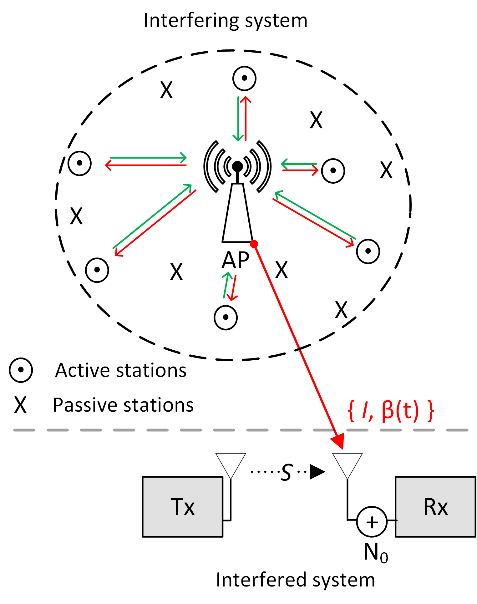
Figure 1: System model for heterogeneous coexistence

II-A Packet Collision Model for an Interfered Sensor Link

Now we develop a packet collision model for the sensor link under the effect of packet arrival process of the WLAN system.

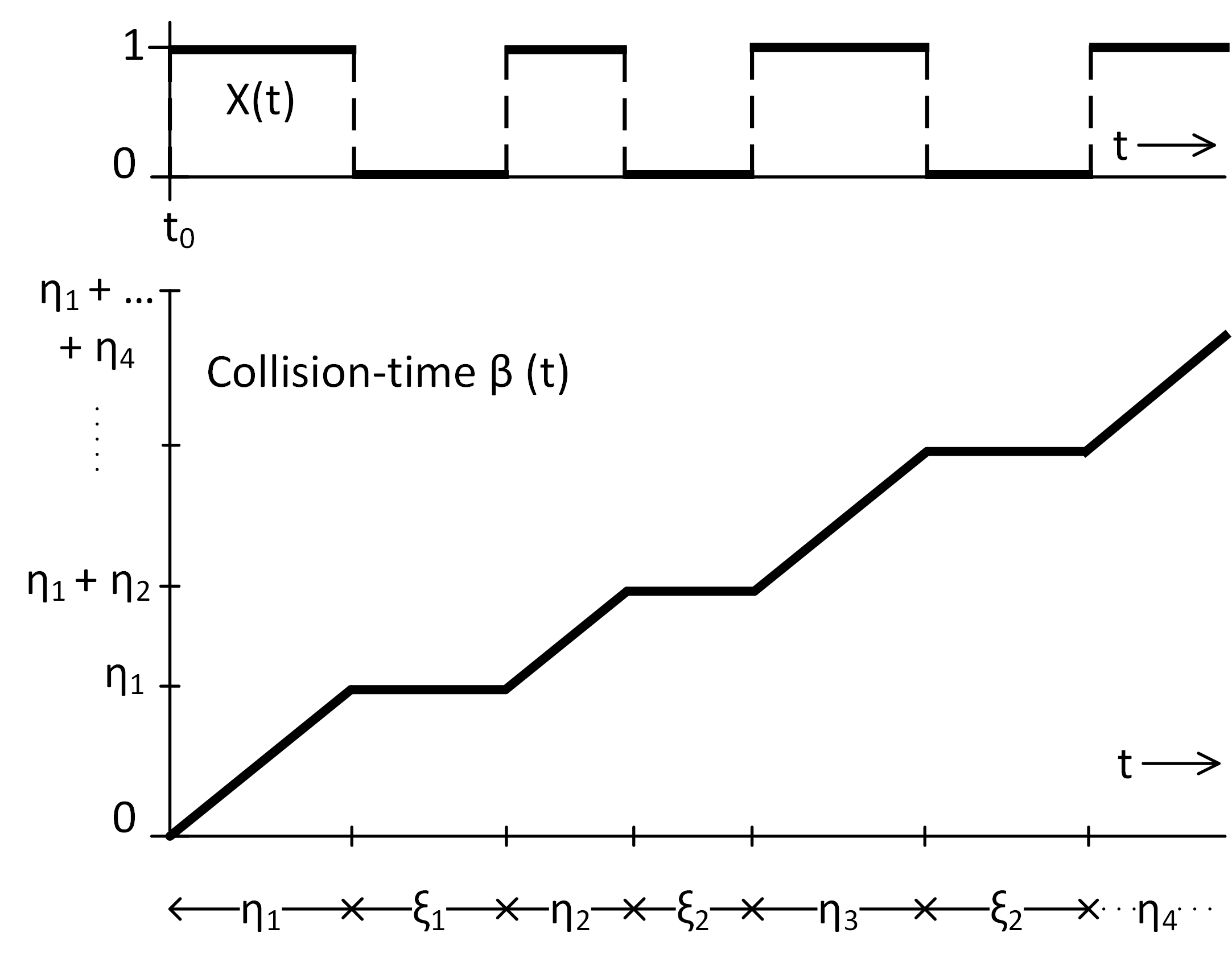
Figure 2: Sample functions of WLAN traffic and collision time processes

Consider an alternating renewal process representing WLAN packet arrivals. At any time instant, the process is in one of the two states: busy (on) or idle (off) (see Fig. 2). Denote the state of the process at time $t\geq 0$ by $\chi(t)$, and let $\chi(t)=1$ if the process is on and $\chi(t)=0$ if it is off. The time evolution of the process is then described by the two state stochastic process $\{\chi(t),t\geq 0\}$. The total on time in which the process spends in state $\chi(t)=1$ during the time interval $(t_{0},t)$ is a stochastic process, denoted as $\beta(t)$, and it is the potential collision time for a sensor link. Mathematically, $\beta(t)$ in terms of $\chi(t)$ is defined as

$$\beta\left(t\right)=\int\limits_{t_{0}}^{t}\chi\left(x\right)\textnormal{d}x$$

The complement of $\beta(t)$ is the total off time, which is the time the process is spends in the state $\chi(t)=0$ during $(t_{0},t)$, and follows $\alpha\left(t\right)=t-\beta\left(t\right)$.

Let variables $\eta_{i}(\xi_{i})$ denote the time spent in state on(off) during the $i$th visit to that state. We assume that all $\eta_{i}(\xi_{i})$ are independent and identically distributed as $\eta(\xi)$ according to $H\left(x\right)=\Pr\{\eta\leq x\}\left(G\left(x\right)=\Pr\{\xi\leq x\}\right)$, and both $\eta$ and $\xi$ are continuous random variables with mean $\bar{\eta}$ and $\bar{\xi}$. The distribution of the sum $\eta_{1}+\eta_{2}+\cdots+\eta_{n}$ is the $n$-fold convolution of $H(x)$, i.e.

$$H_{n}\left(x\right)=\Pr\Big{\{}\sum\limits_{i=1}^{n}\eta_{i}\leq x\Big{\}}$$

where $H_{0}\left(x\right)=1$. An analogous definition holds for $G_{n}\left(x\right)$, being the $n$-fold convolution of $G(x)$. A symbolic representation of the functions $\chi(t)$ and $\beta(t)$ is shown in Fig. 2

Assuming the process enters the state on at time $t_{0}$, the cumulative distribution function (CDF) of the on time, $\beta\left(t\right)$, is given by Takács [7]

$$\Pr\left\{\beta\left(t\right)\leq x\right\}=\sum_{n=0}^{\infty}{H}_{n}\left(x\right)\Pr\{N\left(t-x\right)=n\}$$ (1)

where $\Pr\{N\left(t-x\right)=n\}$, is the probability mass function (PMF) of the number of renewals (or the idle-times) during the time interval $(t_{0},t-x)$ with $x$- the collision time. From [8], the PMF is related to $G_{n}(x)$ as

$$\Pr\{N\left(t-x\right)=n\}=G_{n}\left(t-x\right)-G_{n+1}\left(t-x\right)$$ (2)

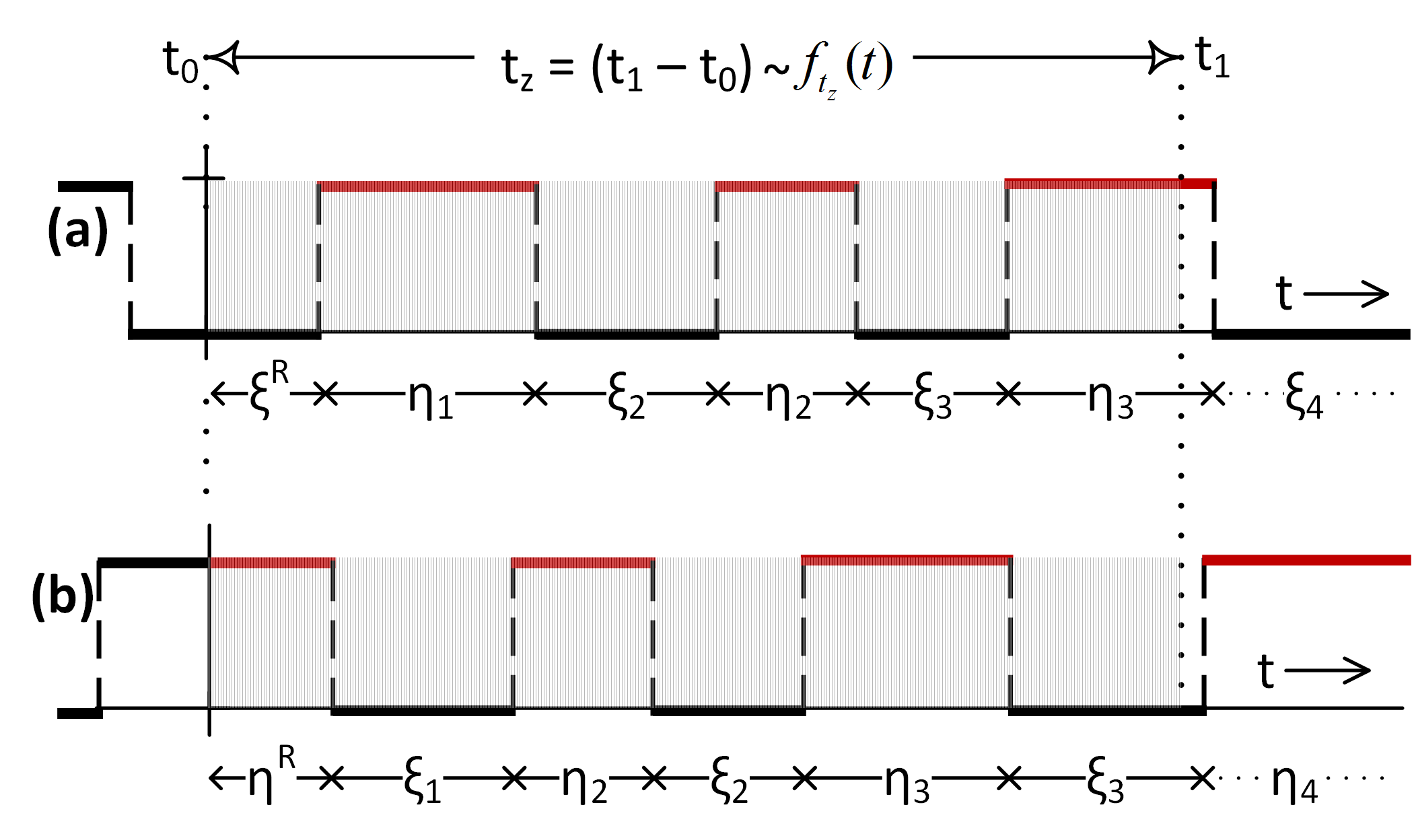
Figure 3: State of the alternating renewal process at observation instant: (a) there is no WLAN packet at the observation instant $t_{0}$ (that is, at the start of a transmission over the sensor link), (b) there is an ongoing WLAN packet transmission at $t_{0}$. The shaded area represents length of the interfered packet which follows a distribution.

From an interfered system’s perspective, the process $\chi\left(t\right)$ however can be in an arbitrary state at time instant $t_{0}$ (see Fig. 3). As a result, at $t_{0}$ the $\chi\left(t\right)$ can be in either state on or off as shown in Fig. 3(a) and Fig. 3(b). Define $\eta^{R}$ and $\xi^{R}$ be the residual time of $\xi$ and $\eta$ with distribution function $H^{R}=\Pr\{\eta^{R}\leq x\}$ and $G^{R}=\Pr\{\xi^{R}\leq x\}$ respectively. Then, the distribution of the sum $\eta^{R}+\eta_{2}+\cdots+\eta_{n}$ is

$$H_{n}^{R}\left(x\right) =H^{R}(x)\ast H_{n}(x)$$

$$=\Pr\Big{\{}\eta^{R}+\sum\limits_{i=2}^{n}\eta_{i}\leq x\Big{\}}$$ (3)

with $H_{0}^{R}\left(x\right)=1$ and $H_{1}^{R}\left(x\right)=H^{R}\left(x\right)$. An analogous definition holds for $G_{n}^{R}\left(x\right)$, being the convolution of $G_{n}(x)$ with $G^{R}(x)$.

Now consider the packet length, $t_{z}$, of the interfered system is a random variable, independent of the random variables $\eta$ and $\xi$, with probability density function (pdf) $f_{t_{z}}(t)$. If $\chi\left(t_{0}\right)=0$, the CDF of on time (i.e., the collision-time distribution of the sensor link), $\omega_{0}\left(x\right)$, can be determined from (1) as

$$\omega_{0}\left(x\right) =\sum_{n=0}^{\infty}{H}_{n}\left(x\right)\!\!\int_{0}^{\infty}\!\!\!\Pr\{N^{e}\left(t-x\right)=n\}f_{t_{z}}(t)\textnormal{d}t$$

$$=\sum_{n=0}^{\infty}{H}_{n}\left(x\right)\Pr\{N_{t_{z}}^{e}\left(x\right)=n\}$$ (4)

where from (3) and (2), $\Pr\{N^{e}\left(t-x\right)=n\}=G_{n}^{R}\left(t-x\right)-G^{R}_{n+1}\left(t-x\right)$ is the PMF of number of renewals in an equilibrium renewal process over a fixed time and $\Pr\{N_{t_{z}}^{e}\left(x\right)=n\}$ is the same measure in a random time.

On the other hand, if $\chi\left(t_{0}\right)=1$, the collision-time distribution, $\omega_{1}\left(x\right)$, from (1) is

$$\omega_{1}\left(x\right) =\sum_{n=0}^{\infty}{H}_{n}^{R}\left(x\right)\!\!\int_{0}^{\infty}\!\!\!\Pr\{N^{o}(t-x)=n\}f_{t_{z}}(t)\textnormal{d}t$$

$$=\sum_{n=0}^{\infty}{H}_{n}^{R}\left(x\right)\Pr\{N_{t_{z}}^{o}\left(x\right)=n\}$$ (5)

where $\Pr\{N^{o}(t-x)=n\}=G_{n}\left(t-x\right)-G_{n+1}\left(t-x\right)$ corresponds to the PMF of the number of renewals in an ordinary renewal process in a fixed time and $\Pr\{N_{t_{z}}^{o}\left(x\right)=n\}$ denotes the PMF in a random time.

As, at an arbitrary time instant $t_{0}>0$, we find the system in on state with probability $\Pr\left\{\chi\left(t_{0}\right)=1\right\}=\frac{\bar{\eta}}{\bar{\eta}+\bar{\xi}}\triangleq\alpha$ and in off state with probability $1-\alpha$, the joint collision-time distribution function is

$$\Omega\left(x\right)\triangleq\alpha\omega_{1}\left(x\right)+\left(1-\alpha\right)\omega_{0}\left(x\right).$$ (6)

III Collision Time Analysis

In this section, for a random packet length $t_{z}$ we find the on time distributions, ${H}_{n}\left(x\right)$ and ${H}_{n}^{R}\left(x\right)$, and the PMF of the number of renewals, $\Pr\{N_{t_{z}}^{e}\left(x\right)=n\}$ and $\Pr\{N_{t_{z}}^{o}\left(x\right)=n\}$, assuming various on- and off-time distributions of the WLAN system.

III-A Interference On Time Distribution

The packet transmission time, which depends on the packet length and the bit rate, corresponds to the on time of an alternating renewal process. In the following, we consider constant and exponentially distributed on time without the loss of generality.

III-A1 Constant packet length

Assuming a constant WLAN packet length (i.e., $\bar{\eta}=t_{w}$), the on time distribution is given by [5]

$${H}_{n}\left(x\right)=\begin{cases}0,&x<nt_{w}\\ 1,&x\geq nt_{w}\end{cases}$$ (7)

Since the residual time, $\eta^{R}$ is uniformly distributed in the interval $\left[0,t_{w}\right]$, we have [5]

$${H}_{n}^{R}\left(x\right)=\begin{cases}0,&x<\left(n-1\right)t_{w}\\ {\frac{{x-(n-1)T}}{{T}}},&\left(n-1\right)T\leq x<nt_{w}\\ 1,&x\geq nt_{w}\end{cases}$$ (8)

III-A2 Random packet length

On the other hand, if $t_{w}$ follows the exponential distribution with parameter $\mu$ and mean $\bar{\eta}=1/\mu$, ${H}_{n}\left(x\right)={H}_{n}^{R}\left(x\right)$ is the Erlang-$n$ distribution

$${H}_{n}\left(x\right)={H}_{n}^{R}\left(x\right)=1-\sum\limits_{k=0}^{n-1}\frac{1}{k!}\left(\mu x\right)^{k}{\rm{exp}}\left(-\mu x\right)$$ (9)

III-B PMF of Number of Renewals

Let $P(t,z)$ be the probability generating function (PGF) of $N_{t}$, the number of renewals in a fixed interval in $(0,t)$, defined as

$$P(t,z)=\mathbf{E}\left[z^{N_{t}}\right]=\sum_{n=0}^{\infty}\Pr\{N_{t}=n\}z^{n}$$ (10)

Then $P(z)$, the PGF of $N_{t_{z}}$ i.e., the number of renewals in a random interval in $(0,t_{z})$ with PDF $f_{t_{z}}(t)$, is

$$P(z)=\int_{0}^{\infty}P(t,z)f_{t_{z}}(t)dt$$ (11)

The PMF of $N_{t_{z}}$ from (11) can be determined as

$$\Pr\{N_{t_{z}}=n\}=\frac{1}{n!}\frac{d^{n}}{dz^{n}}P\left(z\right)\Big{\rvert}_{z=0},n=0,1,2,...$$ (12)

With the basic relations in place in (10)-(12), we find $\Pr\{N_{t_{z}}^{e}\left(x\right)=n\}$ and $\Pr\{N_{t_{z}}^{o}\left(x\right)=n\}$ need in (4) and (5). The PGF of the number of renewals in a fixed interval assumes a general form [8, eq. (3.2.2)]

$$P(t-x,z)=1+\sum_{n=1}^{\infty}{z^{n-1}(z-1)\{G_{n}(t-x)\}^{n}}$$ (13)

Now if the Laplace transform of $g_{n}(t)$ is $g^{*}_{n}(s)$, then that of $G_{n}(t-x)$ is $g^{*}_{n}(s)e^{-sx}/s$. The function $g^{*}_{n}(s)$ for ordinary and equilibrium renewal process is equal to $\{g^{*}(s)\}^{n}/s$ and to $\{1-g^{*}(s)\}\{g^{*}(s)\}^{n-1}/(\bar{\xi}s)$ respectively. Therefore, the Laplace transform of (13) for equilibrium renewal process is

$$P_{e}^{*}(s,z)=\frac{1}{s}+\frac{(z-1)\{1-g^{*}(s)\}}{\bar{\xi}s^{2}\{1-zg^{*}(s)\}}e^{-sx}$$ (14)

while for ordinary renewal process we have

$$P_{o}^{*}(s,z)=\frac{1-g^{*}(s)}{s\{1-zg^{*}(s)\}}e^{-sx}$$ (15)

Assuming $t_{z}$ is exponential distributed with parameter $\lambda_{z}$, from [8, eq. (3.4.3)] the (14) and (15) can easily be inverted with

$$P_{\{e,o\}}(z)=\lambda_{z}P_{\{e,o\}}^{*}(s,z)\Big{\rvert}_{s=\lambda_{z}}$$ (16)

Now by substituting (14) and (15) in (16), one can find the PMFs of the number of renewals desired in (4) and (5) with (12). We find that the PMF of number of renewals in (4) is

$$\Pr\{N_{t_{z}}^{e}\left(x\right)=n\}$$

$$\!\!\!\!=\begin{dcases}1-\left[\frac{\{1-g^{*}(s)\}e^{-sx}}{s\bar{\xi}}\right]_{s=\lambda_{z}},&\mkern-18.0mu\mkern-18.0mu\mkern-18.0mu\mkern-18.0mun=0\\ \left[\frac{e^{-sx}}{s\bar{\xi}}\left(\{g^{*}(s)\}^{n+1}\!\!-\!2\{g^{*}(s)\}^{n}\!\!+\!\{g^{*}(s)\}^{n-1}\right)\!\right]_{s=\lambda_{z}}\!\!\!\!,\\ &\mkern-18.0mu\mkern-18.0mu\mkern-18.0mu\mkern-18.0mun\geq 1\end{dcases}$$ (17)

while the PMF in (5) is

$$\Pr\{N_{t_{z}}^{o}\left(x\right)=n\}$$

$$=\begin{dcases}1-\left[{e^{-sx}g^{*}(s)}\right]_{s=\lambda_{z}},&n=0\\ \left[e^{-sx}\left(\{g^{*}(s)\}^{n}-\{g^{*}(s)\}^{n+1}\right)\right]_{s=\lambda_{z}},&n\geq 1\end{dcases}$$ (18)

For any idle-time distribution of WLAN traffic with known Laplace transform, one can easily find the PMF of the number of renewals observed during a packet duration over the sensor link from (17) and (18). In the following, we consider the exponential and hyperexponential idle-time distributions (without loss of generality) as examples.

III-B1 Exponential idle times

The Laplace transform of exponential distribution with parameter $\rho$ is $g^{*}(s):=\frac{\rho}{s+\rho}$, and the distribution of the renewals is

$$\Pr\{N_{t_{z}}^{e}\left(x\right)=n\}=\Pr\{N_{t_{z}}^{o}\left(x\right)=n\}$$

$$=\begin{dcases}1-\frac{\rho e^{-\lambda_{z}x}}{\lambda_{z}+\rho},&n=0\\ e^{-\lambda_{z}x}\left(\frac{\rho}{\lambda_{z}+\rho}\right)^{n-1}\left(\frac{\lambda_{z}}{\lambda_{z}+\rho}\right),&n\geq 1\end{dcases}$$ (19)

III-B2 Hyperexponential idle time

The hyperexponential distribution is the mixture of $k$ exponential random variables, i.e.

$$g(x)=\sum_{i=1}^{k}{p_{i}\rho_{i}e^{-\rho_{i}x}}$$ (20)

where $\sum_{i=1}^{k}p_{i}=1$ and $E[X]=\sum_{i=1}^{k}{p_{i}}/{\rho_{i}}$. The Laplace transform of hyperexponential PDF is,

$$g^{*}(s)=\sum_{i=1}^{M}p_{i}\frac{\rho_{i}}{s+\rho_{i}}$$ (21)

Substituting (21) into (17) and (18), it is straightforward to find the desired expressions of PMFs, which are excluded here due to space limitations.

III-C Numerical Validation

We validate the proposed CTD in (6) with the distributions developed in Section  III-A & III-B respectively. We assume that mean interfered packet transmission time is $\bar{t}_{z}=1/\lambda_{z}=1.984$ $m$s equaling a packet size of 60 bytes at 256 kbps whereas WLAN busy-time is constant with $t_{w}=374$ $\mu$s which is equivalent of a nominal packet size of 500 bytes at 12 Mbps. Also, we assume that the idle-time is exponentially distributed. For validation, the numerical results from (6) are compared against Matlab simulations, and shown in Fig. 4 for $\alpha=0.0361$ and $\alpha=0.1575$. It can be observed that the numerical results are in excellent agreement with the simulations both for the low and high channel activity factors. Note that $y-$intercept is the probability of having no collisions with WLAN traffic during the interfered packet duration.

After validating the proposed model, we look at the collision-time distributions under realistic hyperexponential idle-time distribution of WLAN. For this purpose, the hyperexpoential distribution parameters are taken from [2] that fit best, based on the algorithm in [9], to the idle-time measurements taken from a real environment with heterogeneous WLANs/Bluetooth at 2.4 GHz. The fitted hyperexponential parameters with respect to the observed spectrum activity factor ($\alpha$) are given in Table I. For the measurement setup and other details, the reader can refer to [2]. Again, assuming the $\bar{t}_{z}=1/\lambda_{z}=1.984$ $m$s and $t_{w}=374$ $\mu$s, the numerical CTD is plotted in Fig. 5. A number of observations can be made from Fig. 5. As the activity factor increases the probability of collisions and the collision time increases. However owing to the long-tailed behavior in hyperexponential case, the probability of no collision remains smaller than the exponential case with the same activity factor.

TABLE I: Estimated Parameters for Hyperexponentially Distributed Idle Times [2]

	$\alpha<0.1$	$\alpha\in[0.1,0.3]$	$\alpha\in[0.3,0.5]$	$\alpha\geq 0.5$
$1/\lambda_{1}$	0.040380	0.022490	0.012690	0.014890
$1/\lambda_{2}$	0.01174	0.006445	0.003289	0.002606
$1/\lambda_{3}$	0.00468	0.000388	0.000457	0.000395
$p_{1}$	0.328	0.093	0.037	0.012
$p_{2}$	0.356	0.577	0.467	0.176
$p_{3}$	0.316	0.330	0.496	0.812

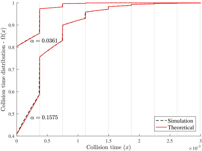
Figure 4: Collision-time distribution under exponential channel idle-times

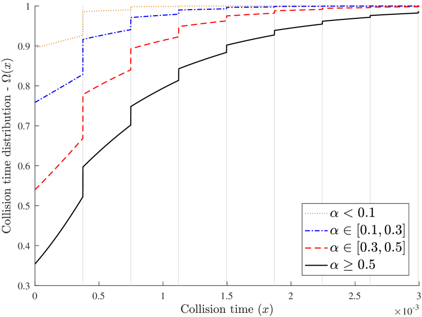
Figure 5: Collision-time distribution under hyperexponential channel idle-times

IV Packet Error Analysis under $\beta(t)$

Depending on the composite traffic arrival process, $\beta(t)$ and the packet length of the sensor link, the number of interfered bits follow the collision-time distribution which we derived in the previous sections. In order to analyze the packet error performance under an observed $\beta(t)$, now we develop a packet error rate model (PER).

IV-A PER Model

We assume that (in general) the downlink traffic from the WLAN AP to the stations outweighs the uplink traffic. In addition, when the WLAN stations are approximately at the same distance relative to the sensor system, it can be assumed that the interference power experienced by the sensor link is equivalent to the interference $I$ from the AP (see Fig. 1). Furthermore, we consider the case where the desired signal undergoes constant channel gain as in [10], while the WLAN interfering signal is subject to Rayleigh multipath fading. Therefore, without WLAN interference, the received signal-to-noise ratio (SNR) of the sensor link is $\gamma_{s}=E_{s}/N_{0}$ where $E_{s}$ is the bit energy of the desired signal and $N_{0}$ the noise power. Whereas in the presence of interference, the received SINR is $\gamma_{c}={\gamma_{s}}/{(1+\gamma_{I})}$ [11] where $\gamma_{I}=|h_{I}|^{2}E_{I}/N_{o}$ is the instantaneous interference-to-noise-ratio (INR) of the interfering signal with $\bar{\gamma}_{I}=E_{I}/N_{o}$ the average INR. Here, $h_{I}$ is the complex channel gain between the WLAN signal and the sensor receiver (with its envelop following the Rayleigh distribution). Therefore, $\gamma_{I}$ is exponentially distributed with the PDF, $f_{\gamma_{I}}=\frac{1}{\bar{\gamma}_{I}}\exp\left(-\gamma_{I}/\bar{\gamma}_{I}\right)$.

$$P_{e}(\gamma,\bar{\gamma}_{I})=1-\sum\limits_{\ell=0}^{N=\infty}\big{(}q_{0}\left(\gamma_{s}\right)\big{)}^{N-\ell}\int_{0}^{\infty}\Big{(}q_{1}\left({\gamma_{s}}/{\gamma_{I}}\right)\Big{)}^{\ell}f_{\gamma_{I}}{d}\gamma_{I}\Big{(}\Omega\left(\ell t_{b}\right)-\Omega\left(\left(\ell-1\right)t_{b}\right)\Big{)}$$ (22)

Consider the packet transmission time of the sensor link $t_{z}$ is exponentially distributed. If the $t_{b}$ is the physical layer bit duration, the number of bits in a packet are $N=[0,\infty$]. Let $b_{e}(\gamma)$ be the BER in AWGN channel which has general form for M-ASK, M-PAM, MSK, M-PSK and M-QAM modulations as

$$b_{e}(\gamma)=c_{m}Q\left(\sqrt{k_{m}\gamma}\right)$$ (23)

where $c_{m}$ and $k_{m}$ are the modulation-specific constants, and $Q(\cdot)$ is the Gaussian $Q$-function. Define $q_{0}\left(\gamma_{s}\right)=1-b_{e}\left(\gamma_{s}\right)$ be the bit success probability when there is no interference, and $q_{1}\left({\gamma_{s}}/{\gamma_{I}}\right)=1-b_{e}\left({\gamma_{s}}/{(1+\gamma_{I})}\right)$ be the bit success probability under interference. The PER of an $N$-bit packet with $\ell$ interfered number of bits is then given by

$$P_{e}(\gamma_{s},\!\bar{\gamma}_{I})\!=\!1\!-\!\big{(}q_{0}\left(\gamma_{s}\right)\big{)}^{\!\!N-\ell}\!\!\!\!\int_{0}^{\infty}\!\!\!\!\Big{(}\!q_{1}\!\left({\gamma_{s}}/{\gamma_{I}}\right)\!\Big{)}^{\ell}\!\!f_{\gamma_{I}}{d}\gamma_{I}$$ (24)

Under $\beta(t)$, $\ell$ will follow a distribution, and the PER model (24) can be reformulated as in (22), where $\Omega\left(x\right)$ is the collision time distribution defined in (6) with $x$ the collision time. Note that $\Omega\left(x\right)=0$ for $x<0$. We assume that the level of interference at the sensor receiver is such that the effect of thermal noise on link performance can be ignored.

IV-B PER Approximations

In this section, we develop approximations for the integral in (22), which using (23) is

$$I_{\ell}=\int_{0}^{\infty}\Big{(}1-c_{m}Q\Big{(}\sqrt{{k_{m}\gamma_{s}}/{\gamma_{I}}}\Big{)}\Big{)}^{\ell}f_{\gamma_{I}}{d}\gamma_{I}$$ (25)

Due to the polynomial of degree $\ell$, the integral in (25) is difficult to evaluate without using $Q$-function approximations. One can apply the binomial expansion to the term $(1-Q(x))^{\ell}$ and use either $Q^{N}$ approximation [12] or exponential function based bounds to $Q$-function [13][14]. However, the approximation in [13] is not accurate and approximation in [14] is not integrable with respect to $\gamma_{I}$ for $\ell\geq 2$ in Rayleigh fading [12]. Therefore, we used the $Q^{N}$ approximation [12]

$$Q^{\ell}(x)\simeq\sum_{k_{1},k_{2},\cdots,k_{n_{a}}}{K_{\ell}C_{\ell}x^{f_{m}}e^{\frac{-{\ell}x^{2}}{2}}}$$ (26)

where the summation is carried over all sequences of non-negative integers $k_{1}+\cdots+k_{n_{a}}=\ell$ and, $K_{\ell}$, $C_{\ell}$ and $f_{m}$ are defined after [12, (4)-(6)]. Note that, the accuracy of (26) depends on $n_{a}$ with $n_{a}=8$ being the reasonable choice. With binomial expansion and using (26), the integral (25) is evaluated as in (29), where $\delta=\frac{1}{4}\left(2-f_{m}\right)$ and $K_{n}(\cdot,\cdot)$ is the modified Bessel function of the second kind.

The approximation in (29) is tight as shown in the Fig. 6, however, it is computationally intensive for higher integer powers ($\ell\geq 8$) of the $Q$-function due to the fact that summation is carried over all sequences of non-negative integers $k_{1},k_{2},\cdots,k_{8}$ that sum to $\ell$. As a result, we utilized an extreme value theory based approximation proposed in [15] for higher powers. From [15], the integrand in (25), denote as $I(x)$, can be as asymptotically approximated by the Gumbel distribution function for the sample maximum as

$$I(x)\simeq\mathrm{exp}\Big{(}\!\!-\mathrm{exp}\Big{(}-\frac{x-a_{\ell}}{b_{\ell}}\Big{)}\Big{)}$$ (27)

where $a_{\ell}=\frac{2}{k_{m}}\big{[}\mathrm{erf}^{-1}\big{(}1-\frac{2}{{\ell}c_{m}}\big{)}\big{]}^{2}$ and $b_{\ell}=\frac{2}{k_{m}}\big{[}\mathrm{erf}^{-1}\big{(}1-\frac{2}{{\ell}c_{m}e}\big{)}\big{]}^{2}-a_{\ell}$ are the normalizing constants, $e$ is the base of the natural logarithm and $\mathrm{erf}^{-1}(\cdot)$ is the inverse error function.

The approximation in (27) is still not integrable in (25). However, Gumbel distribution function (27) can be tightly approximated by the CDF of Gamma distribution by matching the first two moments:

$$\kappa_{\ell}=\frac{6\left(a_{\ell}+b_{\ell}E_{0}\right)^{2}}{\pi^{2}b_{\ell}^{2}},\theta_{\ell}=\frac{a_{\ell}+b_{\ell}E_{0}}{\kappa_{\ell}}$$

where $E_{0}=0.5772$ is the Euler constant. Using the CDF of Gamma distribution, the integral in (25) becomes

$$I_{\ell}=\frac{1}{{\Gamma(\kappa_{\ell})}}\int_{0}^{\infty}{\acute{\gamma}\left(\kappa_{\ell},\frac{\gamma_{s}}{\theta_{\ell}\gamma_{I}}\right)}f_{\gamma_{I}}{d}\gamma_{I}$$ (28)

where $\acute{\gamma}\left(.,.\right)$ and $\Gamma(\cdot)$ stand for lower incomplete and complete Gamma functions respectively [16, p.892]. The integral in (28) over the exponential PDF, we get (30), where $K_{n}(\cdot,\cdot)$ is the modified Bessel function of the second kind.

$$I_{\ell}=1+\frac{1}{\bar{\gamma}_{I}}\sum_{r=1}^{\ell}{{\binom{\ell}{r}}\left(-c_{m}\right)^{r}\sum_{k_{1},k_{2},\cdots,k_{n_{a}}}K_{r}C_{r}2^{1-\delta}\Big{(}rk_{m}\gamma_{s}\bar{\gamma}_{I}\Big{)}^{\delta}\Big{(}k_{m}\gamma_{s}\Big{)}^{1-2\delta}K_{n}\left(-2\delta,\frac{\sqrt{2rk_{m}\gamma_{s}}}{\sqrt{\bar{\gamma}_{I}}}\right)}\vspace{-5pt}$$ (29)

$$I_{\ell}=\frac{1}{\Gamma\left(\kappa_{\ell}\right)}\left(\Gamma\left(\kappa_{\ell}\right)-2\left(\frac{\gamma_{s}}{\bar{\gamma}_{I}\theta_{\ell}}\right)^{\frac{\kappa_{\ell}}{2}}K_{n}\left(-\kappa_{\ell},2\sqrt{\frac{\gamma_{s}}{\bar{\gamma}_{I}\theta_{\ell}}}\right)\right)$$ (30)

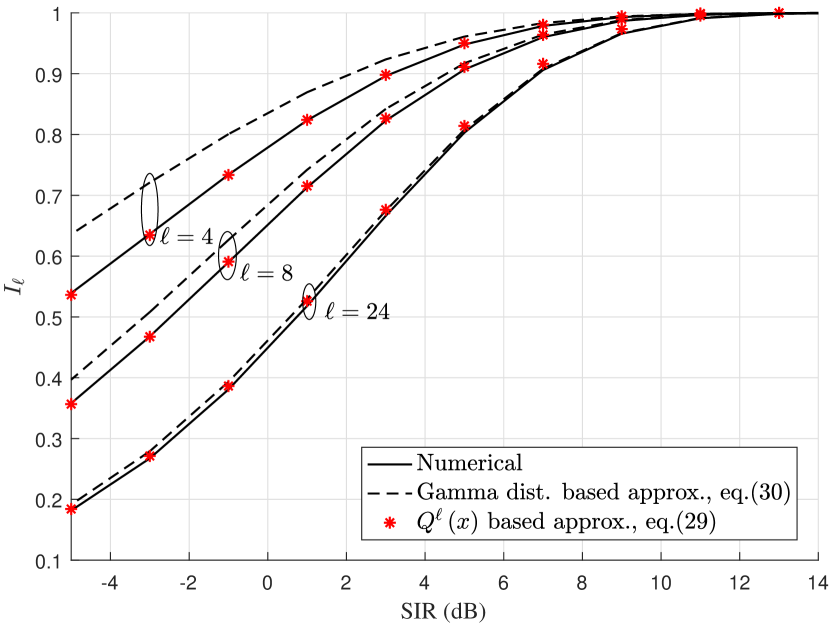
Figure 6: Comparing $I_{\ell}$ approximations for different values of $\ell$ with $c_{m}=1$ and $k_{m}=2$.

Fig. 6 compares the proposed approximations of $I_{\ell}$ in (29) and (30) for different values of $\ell$. It can be observed that approximation (29) is quite tight however its computational demanding. On the other hand, as the number of interfered bits ($\ell$) increase, the tightness of the approximation in (30) also increases suggesting its usage for higher $\ell$.

In Fig. 7, the PER in (22) is evaluated under the collision-time distribution with hyperexpoential parameters given in Table  I, and the approximations in (29) and (30). As the approximation in (29) is computationally demanding, we want to compute it for as lower values of $\ell$ as possible and use approximation (30) for higher values. In Fig. 7, for $\ell\leq 8$ we use (29) and $\ell>8$ (30). It can be observed that this approach matches the numerical result tightly for small to large WLAN activity factors.

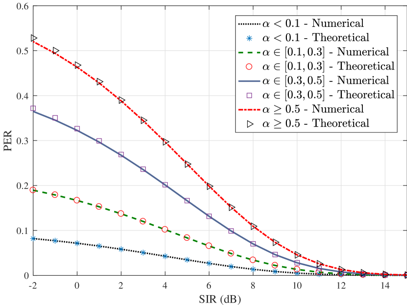
Figure 7: PER of an interfered link under WLAN interference. The modulation parameters of the interfered link are: $c_{m}=1$ and $k_{m}=2$, which correspond to BPSK/QPSK modulation.

V Conclusions

In this paper, we have developed a generic collision-time distribution (CTD) function of an interfered link based on renewal-theoretic modeling of the coexisting traffic. For the exponentially distributed interfered packet lengths, the CTD function is a random sum of the distributions of on-time and number of renewals of the coexisting traffic. The distribution of the number of renewals, which depends on the idle-time statistics, is derived theoretically. The distribution requires only the Laplace transform of the idle-time statistics thus can easily be evaluated for long-tailed hyperexponential or hyper-Erlang distribution. The theoretical collision-time distribution is in excellent agreement with the simulation results. We incorporated the proposed collision- time distribution into a PER model which also takes into account the fading of the interfering signals. We investigated the approximations to PER and derived easy to compute and accurate expressions. As future extension of this work, we would like to study the potential of the packet collision model to RF energy harvesting problems.

References

- [1] A. Ericsson, “Ericsson mobility report: On the pulse of the networked society,” Ericsson, Sweden, Tech. Rep. EAB-14, vol. 61078, 2015.
- [2] L. Stabellini, “Quantifying and modeling spectrum opportunities in a real wireless environment,” in IEEE WCNC. IEEE, 2010, pp. 1–6.
- [3] S. Geirhofer, L. Tong, and B. M. Sadler, “A measurement-based model for dynamic spectrum access in WLAN channels,” in IEEE MILCOM. IEEE, 2006, pp. 1–7.
- [4] S. Y. Shin, H. S. Park, and W. H. Kwon, “Mutual interference analysis of IEEE 802.15.4 and IEEE 802.11b,” Comput. Netw., vol. 51, no. 12, pp. 3338–3353, Aug. 2007.
- [5] A. Mahmood, H. Yigitler, and R. Jäntti, “Stochastic packet collision modeling in coexisting wireless networks for link quality evaluation,” in IEEE ICC, June 2013, pp. 1915–1920.
- [6] S. Lee, R. Zhang, and K. Huang, “Opportunistic wireless energy harvesting in cognitive radio networks,” IEEE Trans. W. Commun., vol. 12, no. 9, pp. 4788–4799, 2013.
- [7] L. Takács, “On certain sojourn time problems in the theory of stochastic processes,” Acta Mathematica Hungarica, vol. 8, pp. 169–191, 1957.
- [8] D. Cox, Renewal Theory. Methuen, 1970.
- [9] A. Feldmann and W. Whitt, “Fitting mixtures of exponentials to long-tail distributions to analyze network performance models,” Performance evaluation, vol. 31, no. 3-4, pp. 245–279, 1998.
- [10] H. Shariatmadari, A. Mahmood, and R. Jantti, “Channel ranking based on packet delivery ratio estimation in wireless sensor networks,” in IEEE WCNC, April 2013, pp. 59–64.
- [11] P. S. Bithas and A. A. Rontogiannis, “Mobile communication systems in the presence of fading/shadowing, noise and interference,” IEEE Trans. Commun., vol. 63, no. 3, pp. 724–737, March 2015.
- [12] Y. Isukapalli and B. D. Rao, “An analytically tractable approximation for the Gaussian Q-function,” IEEE Commun. Lett., vol. 12, no. 9, pp. 669–671, September 2008.
- [13] M. Wu, X. Lin, and P. Y. Kam, “New exponential lower bounds on the Gaussian Q-function via Jensen’s inequality,” in IEEE 73rd Veh. Tech. Conf. (VTC Spring), May 2011, pp. 1–5.
- [14] G. K. Karagiannidis and A. S. Lioumpas, “An improved approximation for the Gaussian Q-function,” IEEE Commun. Lett., vol. 11, no. 8, pp. 644–646, August 2007.
- [15] A. Mahmood and R. Jäntti, “Packet error rate analysis of uncoded schemes in block-fading channels using extreme value theory,” IEEE Commun. Lett., vol. 21, no. 1, pp. 208–211, Jan 2017.
- [16] I. S. Gradshteyn and I. M. Ryzhik, Table of integrals, series, and products, 7th ed. Elsevier, 2007.