Optimizing expected word error rate via sampling for speech recognition

Abstract

State-level minimum Bayes risk (sMBR) training has become the de facto standard for sequence-level training of speech recognition acoustic models. It has an elegant formulation using the expectation semiring, and gives large improvements in word error rate (WER) over models trained solely using cross-entropy (CE) or connectionist temporal classification (CTC). sMBR training optimizes the expected number of frames at which the reference and hypothesized acoustic states differ. It may be preferable to optimize the expected WER, but WER does not interact well with the expectation semiring, and previous approaches based on computing expected WER exactly involve expanding the lattices used during training. In this paper we show how to perform optimization of the expected WER by sampling paths from the lattices used during conventional sMBR training. The gradient of the expected WER is itself an expectation, and so may be approximated using Monte Carlo sampling. We show experimentally that optimizing WER during acoustic model training gives $5\%$ relative improvement in WER over a well-tuned sMBR baseline on a $2$-channel query recognition task (Google Home).

Index Terms: acoustic modeling, sequence training, sampling

1 Introduction

Minimum Bayes risk (MBR) training [1, 2, 3] has been shown to be an effective way to train neural net–based acoustic models and is widely used for state-of-the-art speech recognition systems [4, 5, 6]. MBR training minimizes an expected loss, where the loss measures the distance between a reference and a hypothesis. State-level MBR (sMBR) training [7, 8] is a popular form of MBR training which uses a loss defined at the frame level based on clustered context-dependent phonemes or subphonemes. It is computationally tractable, has an elegant lattice-based formulation using the expectation semiring [9, 10], and has been shown to perform favorably in terms of word error rate (WER) compared to alternative losses that have been proposed [8, 11].

Given the prevalence of word error rate as an evaluation metric, it is natural to consider using it during MBR training. We refer to this as word-level edit-based MBR (word-level EMBR) training. However expected word edit distance over a lattice is harder to compute than the expected frame-level loss used by sMBR training. As a result, many approximations to the true edit distance have been proposed for lattice-based MBR training [2, 12, 13, 7, 8, 14, 15]. Gibson provides a systematic review of the strengths and weaknesses of various approximations [15, chapter 6]. Heigold et al. show that it is possible to exactly compute expected word edit distance over a lattice by first expanding the lattice using an approach sometimes termed error marking [16, 17]. While impressive, error marking is computationally and implementionally non-trivial, and increases the size of the lattices. The memory required for FST determinization during error marking increases rapidly with utterance length, and van Dalen and Gales found a practical limit of around 10 words with the conventional determinization algorithm or around 20 words with an improved, memory-efficient algorithm [17]. The time complexity also means error marking is unlikely to be compatible with on-the-fly lattice generation.

In this paper we propose an alternative approach to lattice-based word-level EMBR training. The gradient of the expected loss optimized by MBR training may itself be written as an expectation, allowing the gradient to be approximated by sampling. The samples are paths through the lattice used during conventional sMBR training. This approach is extremely flexible as it places almost no restriction on the form of loss that may be used. We use this approach to perform word-level EMBR training for two speech recognition tasks and show that this improves WER compared to sMBR training. To our knowledge this is also the first work to investigate word-level EMBR training for state-of-the-art acoustic models based on neural nets.

Similar forms of sampled MBR training have been proposed previously. Graves performed sampled EMBR training for the special case of a CTC model, noting that the special structure of CTC allows trivial sampling and specialized approaches to reduce the variance of the samples [18]. Speech recognition may be viewed as a simple reinforcement learning problem where an action consists of outputting a given word sequence. In this view MBR training is learning a stochastic policy, and the sampling-based approach described here is very similar to the REINFORCE algorithm [19, 20], though here we sample from a probability distribution which is globally normalized instead of locally normalized, and there are differences in the form of variance reduction used.

It should be noted that some previous investigations have reported better WER from optimizing a state-level or phoneme-level criterion than a word-level criterion [2] [15, chapter 7]. However some have reported the opposite [14]. We find the word-level criterion more effective in our experiments but do not investigate this question systematically.

In the remainder of this paper we review the sequence-level probabilistic model used by MBR training (§2 and §3), describe MBR training (§4), discuss EMBR training (§5), describe our sampling-based approach to MBR training (§6), and describe our experimental results (§7).

2 FST-based probabilistic models

In this section we review how a weighted finite state transducer (FST) [21] may be globally normalized to obtain a probabilistic model. The model used for MBR training is defined in this way.

A weighted FST defined over the real semiring (also called the probability semiring) may naturally be turned into a probabilistic model over a sequence of its output labels [22]. Each edge $e$ in the weighted FST has a real-valued weight $w_{e}\geq 0$ and an optional output label taken from a specified output alphabet, and an optional input label taken from a specified input alphabet. The absence of an input or output label is usually denoted with a special epsilon label. A path $\pi$ through the FST from the initial state to the final state consists of a sequence of edges, and the weight of the path $w(\pi)$ is defined as the product $\prod_{e\in\pi}w_{e}$ of the weights of its edges. The probability of a path is defined by globally normalizing this weight function:

$$\mathbb{P}(\pi)=\frac{w(\pi)}{\sum_{\pi}w(\pi)}$$ (1)

This is a Markovian distribution. The output label sequence $\overline{y}(\pi)$ associated with a path $\pi$ is the sequence of non-epsilon output labels along the path. The probability of a sequence $y$ of output labels is defined as the sum of the probabilities of all paths consistent with $y$:

$$\mathbb{P}(y)=\sum_{\pi:\overline{y}(\pi)=y}\mathbb{P}(\pi)$$ (2)

3 Sequence-level model for recognition

In this section we briefly recap a conditional probabilistic model often used for speech recognition. This probabilistic model is an important component in sMBR training.

An acoustic model specifies a mapping $z=\overline{z}(x,\lambda)$ from an acoustic feature vector sequence $x=[x_{t}]_{t=1}^{T}$ to an acoustic logit sequence $z=[z_{t}]_{t=1}^{T}$ given model parameters $\lambda$. Each dimension $q$ of the logit vector $z_{t}=[z_{tq}]_{q=1}^{Q}$ is typically associated with a cluster of context-dependent phonemes or sub-phonemes [23]. In this paper the acoustic model is a stacked long short-term memory (LSTM) network [24]. Given a logit sequence $z$, we define a weighted FST $U(z)$ as the composition

$$U(z)=S(z)\circ(C\circ L\circ G)$$ (3)

of a score FST $S(z)$ and a decoder graph FST $C\circ L\circ G$. The decoder graph is itself a composition and incorporates weighted information about context-dependence (C), pronunciation (L) and word sequence plausibility (G) [25]. The score FST input and output alphabets and the decoder graph input alphabet are $\{1,\ldots,Q\}$. The decoder graph output alphabet is the vocabulary. We refer to $U(z)$ as the unrolled decoder graph since composition with $S(z)$ effectively unrolls the decoder graph over time. The score FST $S(z)$ has a simple “sausage” structure with $T+1$ states and an edge from state $t$ to state $t+1$ with input and output label $q$ and log weight $z_{tq}$ for each frame $t$ and cluster index $q$.

The conditional probabilistic model $\mathbb{P}(y|x,\lambda)$ over a word sequence $y=[y_{j}]_{j=1}^{J}$ given an acoustic feature vector sequence $x=[x_{t}]_{t=1}^{T}$ is obtained by applying the procedure described in §2 to the unrolled decoder graph $U(\overline{z}(x,\lambda))$. This gives

$$\mathbb{P}(\pi|x,\lambda)=\frac{w(\pi,z)}{\sum_{\pi}w(\pi,z)}$$ (4)

where $z=\overline{z}(x,\lambda)$ and $w(\pi,z)$ is the weight of a path.

It will be helpful to know the gradient of the log weight and log probability with respect to the acoustic logits. Due to the way the score FST is constructed, the sequence of non-epsilon input labels encountered along a path through $U(z)$ consists of a cluster index $q_{t}$ for each frame $t\in\{1,\ldots,T\}$. The overall log weight $\log w(\pi,z)$ has an additive contribution $\sum_{t}z_{tq_{t}}$ from the acoustic model, and the gradient $\frac{\partial}{\partial z}\log w(\pi,z)$ consists of a $T\times Q$ matrix which has a one at $(t,q_{t})$ for each frame $t$ and zeros elsewhere. The gradient of the log probability is given by

$$\frac{\partial}{\partial z}\log\mathbb{P}(\pi|z)=\frac{\partial}{\partial z}\log w(\pi,z)-\mathbb{E}\frac{\partial}{\partial z}\log w(\pi,z)$$ (5)

4 Minimum Bayes risk (MBR) training

Minimum Bayes risk (MBR) training [1, 2, 3] minimizes the expected loss

$$\mathbb{E}L(y,y_{\text{ref}})=\sum_{\pi}\mathbb{P}(\pi|x,\lambda)L(\overline{y}(\pi),y_{\text{ref}})$$ (6)

as a function of $\lambda$, where the loss $L(y,y_{\text{ref}})$ specifies how bad it is to output $y$ when the reference word sequence is $y_{\text{ref}}$. Broadly speaking MBR concentrates probability mass: a sufficiently flexible model trained to convergence with MBR will assign a probability of $1$ to the word sequence(s) with smallest loss.

State-level minimum Bayes risk (sMBR) training [7, 8] defines the loss $L(\pi,\pi_{\text{ref}})$, now over $\pi$ instead of $y$, to be the number of frames at which the current cluster index differs from the reference cluster index. The sequence of time-aligned reference cluster indices is typically obtained using forced alignment. This loss has a number of disadvantages compared to minimizing the number of word errors [15, chapter 6]. However it has the advantage that the expected loss and its gradient may be computed tractably using an elegant formulation based on the expectation semiring [9, 10]. The crucial property of the loss $L$ that makes it tractable is that the loss of a path can be decomposed additively over the edges in the path.

Typically it is not feasible to perform sMBR training over the full unrolled decoder graph $U(z)$, and a lattice containing a subset of paths is used instead [27, 4]. There has been some interest recently in performing exact “lattice-free” sequence training using a simplified decoder graph [28].

5 Edit-based MBR (EMBR) training

Given the prevalence of word error rate (WER) as an evaluation metric, a natural loss to use for MBR training is the edit distance between the reference and hypothesized word sequences. We refer to MBR training using a Levenshtein distance as the loss as edit-based MBR (EMBR) training, and to using the number of word errors as word-level EMBR training. The number of word errors is the result of a dynamic programming computation and does not decompose additively over the edges in a path, meaning the expectation semiring approach cannot be applied without modification. As discussed in §1, it is in fact possible to exactly compute the expected number of word errors over a lattice by expanding the lattice using error marking, but this approach produces larger lattices, in practice limits the maximum utterance length, and is not compatible with on-the-fly lattice generation [16, 17].

6 Sampled MBR training

In this section we look at a simple sampling-based approach to computing the MBR loss value and its gradient. This approach is essentially agnostic to the form of loss used, allowing us to perform EMBR training simply and efficiently. We consider the expected loss as a function of $z$ rather than $\lambda$ since this provides the gradients required to implement sampled MBR in a modular graph-of-operations framework such as TensorFlow [29].

Samples from $\mathbb{P}(\pi|z)$ can be drawn efficiently using backward filtering–forward sampling [30]. First the conventional backward algorithm is used to compute the sum $\beta_{i}$ of the weights of all partial paths from each FST state $i$ to the final state. The FST is then reweighted using $\beta$ as a potential function, i.e. replacing the weight $w_{e}$ of each edge $e$, which goes from some state $i$ to some state $j$, with $\beta_{i}^{-1}w_{e}\beta_{j}$ [31]. This results in an equivalent FST which is locally normalized or stochastic, i.e. the sum of edge weights leaving each state is one [31]. Samples from the reweighted FST can be drawn using simple ancestral sampling, i.e. sample an edge leaving the initial state, then an edge leaving the end state of the sampled edge, and repeat until we reach the final state. In our implementation the $\beta$ values are computed once to draw multiple samples and the reweighting is performed on-the-fly during sampling.

We can approximate the expected loss using a straightforward Monte Carlo approximation:

$$\mathbb{E}L(y,y_{\text{ref}}) =\sum_{\pi}\mathbb{P}(\pi|z)L(\overline{y}(\pi),y_{\text{ref}})$$ (7)

$$\approx\frac{1}{I}\sum_{i=1}^{I}L_{i}=\overline{L_{i}}$$ (8)

where each $\pi_{i}$ is an independent sample from $\mathbb{P}(\pi|z)$ and $L_{i}=L(\overline{y}(\pi_{i}),y_{\text{ref}})$. We write $\overline{L_{i}}$ to denote averaging over samples.

The true gradient, writing $L(\pi)$ for $L(\overline{y}(\pi),y_{\text{ref}})$, is

$$\frac{\partial}{\partial z}\mathbb{E}L(\pi) =\frac{\partial}{\partial z}\sum_{\pi}\mathbb{P}(\pi|z)L(\pi)$$ (9)

$$=\sum_{\pi}\mathbb{P}(\pi|z)L(\pi)\frac{\partial}{\partial z}\log\mathbb{P}(\pi|z)$$ (10)

This can be re-expressed using (5) as

$$\mathbb{E}\left[L(\pi)\frac{\partial}{\partial z}\log w(\pi,z)\right]-\mathbb{E}L(\pi)\mathbb{E}\left[\frac{\partial}{\partial z}\log w(\pi,z)\right]$$ (11)

Thus the MBR gradient is a scalar-vector covariance [10], i.e. it is of the form $\mathbb{E}[xy]-\mathbb{E}x\mathbb{E}y$, and an unbiased estimate is

$$\frac{\partial}{\partial z}\mathbb{E}L(\pi)\approx\frac{I}{I-1}\overline{(L_{i}-\overline{L_{i}})\frac{\partial}{\partial z}\log w(\pi_{i},z)}$$ (12)

We refer to using (12) during gradient-based training as sampled MBR training. It has the intuitive interpretation that samples with worse-than-average loss have the log weight of the corresponding path reduced, and samples with better-than-average loss have the log weight of the corresponding path increased. The subtraction of $\overline{L_{i}}$ in (12) makes the estimated gradient invariant to an overall additive shift in loss, and may be seen as performing variance reduction, often regarded as extremely important in sampling-based policy optimization for reinforcement learning [32, 33, 34].

Example code for sampled MBR training is shown in Figure 1. Our implementation consisted of a TensorFlow op with input acoustic logits and output expected loss.

⬇

def mbr(sample_path, collapse_path, get_gammas,

get_loss, num_samples, ref_labels):

paths = [sample_path()

for _ in range(num_samples)]

losses = [

get_loss(collapse_path(path), ref_labels)

for path in paths

]

mean_loss = np.mean(losses)

mean_gammas = sum([

get_gammas(path) * (loss - mean_loss)

for path, loss in zip(paths, losses)

]) / (num_samples - 1)

return mean_loss, mean_gammas

Figure 1: Example python implementation of sampled MBR training. Here sample_path returns a sampled path from a lattice, collapse_path ($\overline{y}$ in (2)) takes a path to a word sequence, get_gammas takes a path to a $T\times Q$ matrix with a one for each (frame, cluster index) which occurs in the path (see §3), and get_loss computes Levenshtein distance in the case of EMBR training.

7 Experiments

We compared sMBR and sampled word-level EMBR training for two model architectures on two speech recognition tasks.

7.1 CTC-style 2-channel Google Home model

We compared the performance of sMBR and EMBR training for a 2-channel query recognition task (Google Home) using a CTC-style model where the set of clustered context-dependent phonemes includes a blank symbol.

Our acoustic feature vector sequence was $480$-dimensional with a $30\,\text{ms}$ frame step, and consisted of a stack of three $10\,\text{ms}$ frames of $80$ log mel filterbanks for each channel. A stacked unidirectional LSTM acoustic model with $5$ layers of $700$ cells each was used, followed by a linear layer with output dimension $8192$ (the number of clusters). These “raw” logits were post-processed by applying log normalization with a softmax-then-log then adding $-1.95$ to the logit for CTC blank and scaling the logits for the remaining clusters by $0.5$ to mimic what is often done during decoding for CTC models; this post-processing does not seem to be critical for good performance. The initial CTC system was trained from a random initialization using $739$ million steps of asynchronous stochastic gradient descent, using context-dependent phonemes as the reference label sequence. The sMBR and EMBR systems were trained for a further $900$ million steps, with the best systems selected by WER on a small held-out dev set being obtained after a total of roughly $1035$ million and $1569$ million steps respectively. For both CTC and MBR training, each step computed the gradient on one whole utterance. Lattices for MBR training were generated on-the-fly. Alignments for sMBR training were computed on-the-fly. The decoder graph used during MBR training was constructed from a weak bigram language model estimated on the training data, and a CTC-style context-dependent C transducer with blank symbol was used [35]. EMBR training used $100$ samples per step. The WER used during EMBR training was computed with language-specific capitalization and punctuation normalization. The learning rate for EMBR training was set $5$ times larger than for sMBR training because the number of word errors is typically smaller than the number of frame errors, and the typical gradient norm values during sMBR and EMBR training reflected this. We verified that using a $5$ times larger learning rate for sMBR was detrimental. The training data was a voice search–specific subset of a corpus of around $20$ million anonymized utterances with artificial room reverbation and noise added. WER was evaluated on three corpora of anonymized $2$-channel Google Home utterances.

WER on the dev set during training is presented in Figure 2. Somewhat contrary to common wisdom that sMBR training converges quickly, we observe WER continuing to improve for around $300$ million steps. After $1$ billion total steps, sMBR training gets worse on the dev set and stays roughly constant on the training set (not shown), meaning it is suffering from overfitting. EMBR training takes a long time to achieve its full gains; indeed it is not clear it has converged even at $1.6$ billion total steps. EMBR performance appears to be as good or better than sMBR after any number of steps. An EMBR step with $100$ samples in our set-up took around the same time as an sMBR step. EMBR has little overhead because sampling paths given the beta probabilities is cheap and because overall computation time for both sMBR and EMBR is typically dominated by the stacked LSTM computations and lattice generation.

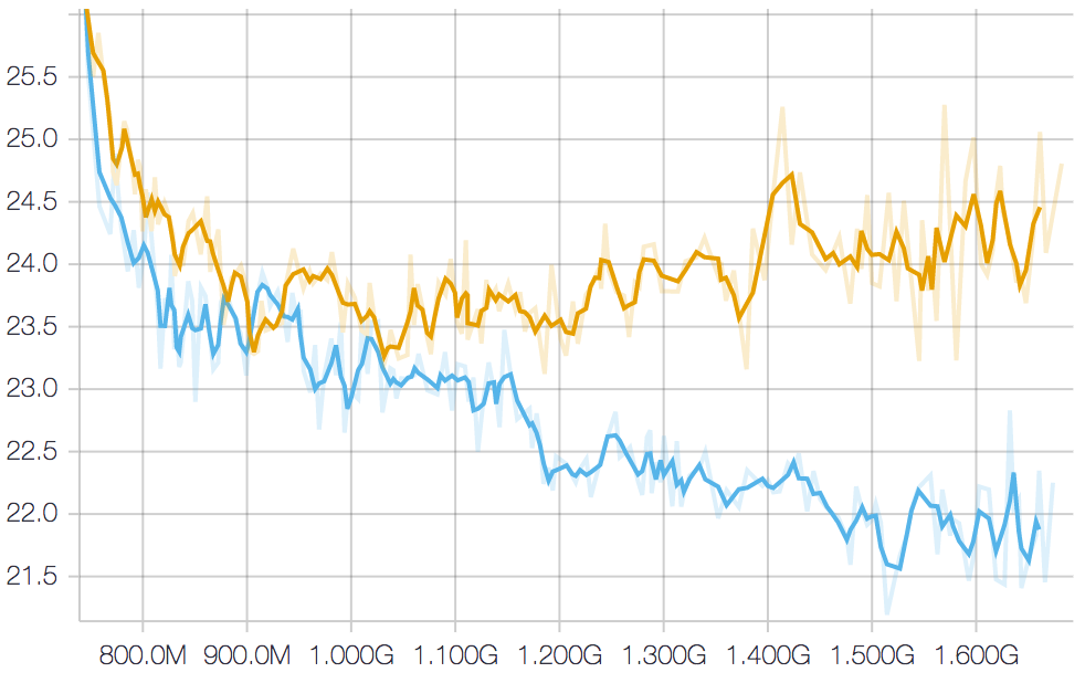
Figure 2: WER computed during training on the dev set for Google Home for sMBR (top) and word-level EMBR (bottom).

The evaluation results are presented in Table 1. We can see the sampled word-level EMBR training gave a 4–5 % relative gain over sMBR training.

Test set	Num utts	WER		Relative
		sMBR	WEMBR
Home 1	21k	6.5	6.2	-5%
Home 2	22k	6.3	5.9	-6%
Home 3	22k	6.9	6.6	-4%
Overall	65k	6.6	6.2	-5%

Table 1: Word error rates for CTC-style 2-channel Google Home model trained with sMBR and word-level EMBR.

7.2 Non-CTC 1-channel voice search model

We also compared the performance of sMBR and EMBR training for a 1-channel voice search task. Our acoustic feature vector sequence was $512$-dimensional with a $30\,\text{ms}$ frame step, and consisted of a stack of four $10\,\text{ms}$ frames of $128$ log mel filterbanks. The stacked LSTM had $5$ layers of $600$ cells each. An initial cross-entropy system was trained for $305$ million steps. The sMBR and EMBR systems were trained for a futher $420$ million steps, and the models with best WER on a held-out dev set were at around $680$ million and $720$ million total steps respectively. The systems were trained on a corpus of around $15$ million anonymized voice search and dictation utterances with artificial reverb and noise added and evaluated on four voice search test sets including one with noise added.

WER on the dev set during training is presented in Figure 3, and results are presented in Table 2. In these experiments we used the same learning rate for sMBR and EMBR training since we were not yet fully aware of the mismatch in dynamic range; using a smaller learning rate may improve sMBR performance. We observed consistent gains from word-level EMBR training on this task.

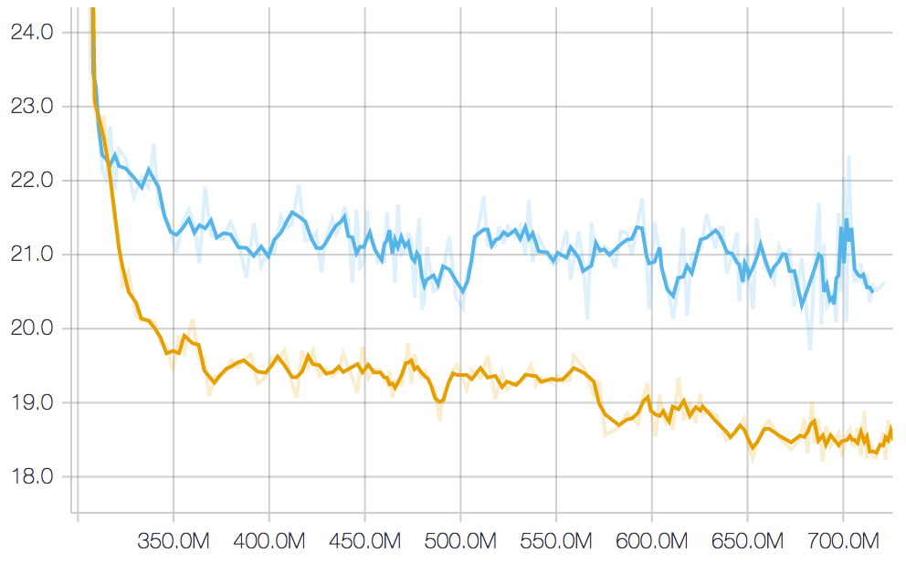
Figure 3: WER computed during training on the dev set for voice search for sMBR (top) and word-level EMBR (bottom).

Test set	Num utts	WER		Relative
		sMBR	WEMBR
VS 0	13k	11.7	11.3	-3%
VS 0 noisified	13k	14.0	13.2	-6%
VS 1	15k	9.4	9.0	-4%
VS 2	22k	10.7	10.2	-5%

Table 2: Word error rates for non-CTC 1-channel voice search model trained with sMBR and word-level EMBR.

8 Conclusion

We have seen that sampled word-level EMBR training provides a simple and effective way to optimize expected word error rate during training, and that this improves empirical performance on two speech recognition tasks with disparate architectures.

9 Acknowledgements

Many thanks to Erik McDermott for his patient and helpful feedback on successive drafts of this manuscript, and to Haşim Sak for many fruitful and enjoyable discussions while implementing sMBR and EMBR training in TensorFlow.

References

- [1] J. Kaiser, B. Horvat, and Z. Kacic, “A novel loss function for the overall risk criterion based discriminative training of HMM models,” in Proc. ICSLP, 2000.
- [2] D. Povey and P. C. Woodland, “Minimum phone error and I-smoothing for improved discriminative training,” in Proc. ICASSP, 2002.
- [3] V. Doumpiotis and W. Byrne, “Pinched lattice minimum Bayes risk discriminative training for large vocabulary continuous speech recognition,” in Proc. Interspeech, 2004.
- [4] B. Kingsbury, “Lattice-based optimization of sequence classification criteria for neural-network acoustic modeling,” in Proc. ICASSP, 2009.
- [5] H. Sak, A. Senior, K. Rao, and F. Beaufays, “Fast and accurate recurrent neural network acoustic models for speech recognition,” in Proc. Interspeech, 2015.
- [6] J. R. Bellegarda and C. Monz, “State of the art in statistical methods for language and speech processing,” Computer Speech & Language, vol. 35, pp. 163–184, 2016.
- [7] M. Gibson and T. Hain, “Hypothesis spaces for minimum Bayes risk training in large vocabulary speech recognition,” in Proc. Interspeech, 2006.
- [8] D. Povey and B. Kingsbury, “Evaluation of proposed modifications to MPE for large scale discriminative training,” in Proc. ICASSP, 2007.
- [9] J. Eisner, “Expectation semirings: Flexible EM for learning finite-state transducers,” in Proc. ESSLLI workshop on finite-state methods in NLP, 2001.
- [10] G. Heigold, T. Deselaers, R. Schlüter, and H. Ney, “Modified MMI/MPE: A direct evaluation of the margin in speech recognition,” in Proc. ICML, 2008.
- [11] K. Veselỳ, A. Ghoshal, L. Burget, and D. Povey, “Sequence-discriminative training of deep neural networks,” in Proc. Interspeech, 2013.
- [12] J. Zheng and A. Stolcke, “Improved discriminative training using phone lattices,” in Proc. Interspeech, 2005.
- [13] W. Macherey, L. Haferkamp, R. Schlüter, and H. Ney, “Investigations on error minimizing training criteria for discriminative training in automatic speech recognition,” in Proc. Interspeech, 2005.
- [14] Z.-J. Yan, B. Zhu, Y. Hu, and R.-H. Wang, “Minimum word classification error training of HMMs for automatic speech recognition,” in Proc. ICASSP, 2008.
- [15] M. Gibson, “Minimum Bayes risk acoustic model estimation and adaptation,” Ph.D. dissertation, University of Sheffield, UK, 2008.
- [16] G. Heigold, W. Macherey, R. Schluter, and H. Ney, “Minimum exact word error training,” in Proc. ASRU, 2005.
- [17] R. C. Van Dalen and M. J. Gales, “Annotating large lattices with the exact word error,” in Proc. Interspeech, 2015.
- [18] A. Graves and N. Jaitly, “Towards end-to-end speech recognition with recurrent neural networks,” in Proc. ICML, 2014.
- [19] R. J. Williams, “Simple statistical gradient-following algorithms for connectionist reinforcement learning,” Machine learning, vol. 8, no. 3-4, pp. 229–256, 1992.
- [20] M. Ranzato, S. Chopra, M. Auli, and W. Zaremba, “Sequence level training with recurrent neural networks,” in Proc. ICLR, 2016.
- [21] M. Mohri, F. Pereira, and M. Riley, “Weighted finite-state transducers in speech recognition,” Computer Speech & Language, vol. 16, no. 1, pp. 69–88, 2002.
- [22] J. Eisner, “Parameter estimation for probabilistic finite-state transducers,” in Proc. Association for Computational Linguistics, 2002.
- [23] G. E. Dahl, D. Yu, L. Deng, and A. Acero, “Context-dependent pre-trained deep neural networks for large-vocabulary speech recognition,” IEEE Transactions on Audio, Speech, and Language Processing, vol. 20, no. 1, pp. 30–42, 2012.
- [24] S. Hochreiter and J. Schmidhuber, “Long short-term memory,” Neural computation, vol. 9, no. 8, pp. 1735–1780, 1997.
- [25] M. Mohri, F. Pereira, and M. Riley, “Speech recognition with weighted finite-state transducers,” in Springer Handbook of Speech Processing, 2008, pp. 559–584.
- [26] V. Goel and W. J. Byrne, “Minimum Bayes-risk automatic speech recognition,” Computer Speech & Language, vol. 14, no. 2, pp. 115–135, 2000.
- [27] V. Valtchev, J. Odell, P. C. Woodland, and S. J. Young, “Lattice-based discriminative training for large vocabulary speech recognition,” in Proc. ICASSP, 1996.
- [28] D. Povey, V. Peddinti, D. Galvez, P. Ghahrmani, V. Manohar, X. Na, Y. Wang, and S. Khudanpur, “Purely sequence-trained neural networks for ASR based on lattice-free MMI,” 2016.
- [29] M. Abadi, P. Barham, J. Chen, Z. Chen, A. Davis, J. Dean, M. Devin, S. Ghemawat, G. Irving, M. Isard et al., “TensorFlow: A system for large-scale machine learning,” in Proc. OSDI, 2016.
- [30] H.-A. Loeliger and M. Molkaraie, “Estimating the partition function of 2-D fields and the capacity of constrained noiseless 2-D channels using tree-based Gibbs sampling,” in Proc. Information Theory Workshop, 2009, pp. 228–232.
- [31] M. Mohri and M. Riley, “A weight pushing algorithm for large vocabulary speech recognition,” in Proc. Interspeech, 2001.
- [32] R. S. Sutton, D. A. McAllester, S. P. Singh, Y. Mansour et al., “Policy gradient methods for reinforcement learning with function approximation,” in NIPS, vol. 99, 1999, pp. 1057–1063.
- [33] F. Sehnke, C. Osendorfer, T. Rückstieß, A. Graves, J. Peters, and J. Schmidhuber, “Parameter-exploring policy gradients,” Neural Networks, vol. 23, no. 4, pp. 551–559, 2010.
- [34] V. Mnih, N. Heess, A. Graves et al., “Recurrent models of visual attention,” in Advances in neural information processing systems, 2014, pp. 2204–2212.
- [35] H. Sak, A. Senior, K. Rao, O. Irsoy, A. Graves, F. Beaufays, and J. Schalkwyk, “Learning acoustic frame labeling for speech recognition with recurrent neural networks,” in Proc. ICASSP, 2015.